1 Angular dependence

The essential parts of this and next section can be found in many references [1]. Here, we attempt to describe central concepts and derive critical expressions as simply as possible.

1.1 Introduction

We consider a two-body decay $0\to a+b$ in the rest frame of the parent particle, where the spin state $(J,M)$ of the parent particle and the helicities $\lambda_{a,b}$ of the daughters are given. The final state with a definite total angular momentum and definite helicities can be constructed as follows: In general, if $|\hat{n}\lambda\rangle$ is a state with total angular momentum $\lambda$ along the direction $\hat{n}$, one can form a state with total angular momentum $|J,M\rangle$ where the quantization axis is taken as the $z$ direction (i.e. in the lab frame), as

$$|JM,\lambda\rangle=\int d\hat{n}\,D^{J*}_{M,\lambda}(\hat{n})\,|\hat{n}\lambda\rangle\,,$$ (1)

with

$$d\hat{n}=d\phi\,d\!\cos\theta\,,\quad D^{j}_{m,m^{\prime}}(\hat{n})=D^{j}_{m,m^{\prime}}(\phi,\theta,0)$$ (2)

where $(\theta,\phi)$ is the polar coordinate of the direction $\hat{n}$, and $D^{j*}_{m,m^{\prime}}(\hat{n})$ is the rotation function, or the wave function of a top with total angular momentum $|JM\rangle$ and the component along $\hat{n}$ given by $\lambda$ which is also a good quantum number.

Suppose $|\hat{p}\lambda_{a}\lambda_{b}\rangle$ is the state in which particle $a$ is moving in the $\hat{p}$ direction with helicity $\lambda_{a}$ and particle $b$ is moving in the $-\hat{p}$ direction with helicity $\lambda_{b}$:

$$|\hat{p}\lambda_{a}\lambda_{b}\rangle=|\hat{p}\lambda_{a}\rangle|-\hat{p}\lambda_{b}\rangle\,.$$ (3)

Then, (1) with the identification

$$\hat{n}=\hat{p}\,,\quad\lambda=\lambda_{a}-\lambda_{b}\,,$$ (4)

gives the state with total angular momentum $|JM\rangle$ and total helicity $\lambda_{a}-\lambda_{b}$ along the direction of $a$:

$$|JM,\lambda_{a}\lambda_{b}\rangle=N\int d\hat{p}\,D^{J*}_{M\,\lambda_{a}-\lambda_{b}}(\hat{p})\,|\hat{p}\lambda_{a}\lambda_{b}\rangle\,,$$ (5)

where $N$ is a normalization factor. The ranges of the integration are

$$-1\leq\cos\theta\leq 1\,,\quad 0\leq\phi\leq 2\pi\,.$$ (6)

The possible values of the heclicities are constrained by

$$|\lambda_{a}-\lambda_{b}|\leq M\,,$$ (7)

which arises since the orbital angular momentum cannot have a component along the line of decay. The construction (5) indicates that the amplitude for particle $a$ to be in direction $\hat{p}$ is $D^{J*}_{M\,\lambda_{a}-\lambda_{b}}(\hat{p})$.

Transformation of the state $|JM,\lambda_{a}\lambda_{b}\rangle$ under parity is given by [2]

$$P|JM,\lambda_{a}\lambda_{b}\rangle=\pi_{a}\pi_{b}(-1)^{J-s_{a}-s_{b}}|JM,-\lambda_{a}-\lambda_{b}\rangle\,,$$ (8)

where $s_{a,b}$ and $\pi_{a,b}$ are the spins and intrinsic parities of the daughter particles, respectively.

1.2 $B\to V_{a}V_{b}$, helicity basis

In $B$ decays of the type $B\to V_{a}V_{b}$ ($V$: a vector), such as $B^{+}\to\Psi K^{*+}$ and $\bar{D}^{*0}\rho^{+}$, we have

$$J=M=0,\quad s_{a}=s_{b}=1,\quad\pi_{a}=\pi_{b}=-1\,.$$ (9)

The constraint (7) with $M=0$ means $\lambda_{a}=\lambda_{b}$, and thus there are three possible helicity states:

$$(\lambda_{a},\lambda_{b})=(+1,+1),\quad(0,0),\quad{\rm or}\;(-1,-1)\,.$$ (10)

Accordingly, the final state can be written as

$$|\Psi_{f}\rangle=\sum_{\lambda}H_{\lambda}\,|f_{\lambda}\,\rangle\quad(\lambda=+1,0,-1)\,,$$ (11)

where $H_{i}$ is the amplitude for each helicity state, and we have defined

$$\begin{array}[]{rcl}|f_{+1}\rangle&\equiv&|JM,+1+1\rangle\,,\\ |f_{0}\rangle&\equiv&|JM,00\rangle\,,\\ |f_{-1}\rangle&\equiv&|JM,-1-1\rangle\,.\end{array}\quad(J=M=0)$$ (12)

In terms of decay amplitude, one can write

$$H_{\lambda}=\langle f_{\lambda}|H_{\rm eff}|B\rangle\,,$$ (13)

where $H_{\rm eff}$ is the effective Hamiltonian responsible for the decay.

When the daughter particles subsquently decay as

$$a\to a_{1}+a_{2}\,,\quad b\to b_{1}+b_{2}\,,$$ (14)

the construction (5) applies to each decay in its rest frame. The decay amplitude for $a_{1}$ to be in direction $(\theta_{a},\phi_{a})$ in the rest frame of $a$ and $b_{1}$ to be in direction $(\theta_{b},\phi_{b})$ in the rest frame of $b$ is then (up to an overall constant)

$$A=\sum_{m}H_{m}\,D^{s_{a}*}_{m,\lambda_{a_{1}}-\lambda_{a_{2}}}(\phi_{a},\theta_{a},0)\,D^{s_{b}*}_{m,\lambda_{b_{1}}-\lambda_{b_{2}}}(\phi_{b},\theta_{b},0)\,.$$ (15)

The $z$ axis in the rest frame of $a$ is taken to be in the direction of $\hat{p}$, and that in the rest frame of $b$ is taken to be in the direction of $-\hat{p}$; namely, each in the direction of the motion of the parent particle in the $B$ frame. The definition of the azimuthal angles amounts to defining the phase convention for the helicity amplitudes $H_{m}$. To be specific, we define that the $x$ directions in the two frames are the same (see Figure 1).

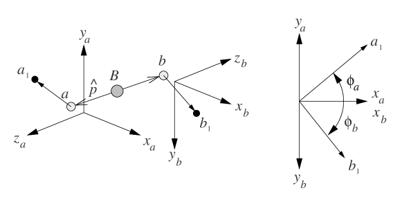
Figure 1: Definition of angles for $B\to V_{a}V_{b}$ decay.

Using

$$D^{j}_{m,m^{\prime}}(\alpha,\beta,\gamma)=e^{-im\alpha}d^{j}_{m,m^{\prime}}(\beta)e^{-im^{\prime}\gamma}\,,$$ (16)

the amplitude can be written as

$$A=\sum_{m}H_{m}\;e^{im\chi}d^{s_{a}}_{m,\lambda_{a_{1}}-\lambda_{a_{2}}}(\theta_{a})d^{s_{b}}_{m,\lambda_{b_{1}}-\lambda_{b_{2}}}(\theta_{b})\,,$$ (17)

with

$$\chi\equiv\phi_{a}+\phi_{b}$$ (18)

being the azimuthal angle from $b_{1}$ to $a_{1}$ measured counter-clock-wise looking down from the $a$ side.

1.3 Transversity basis

Using the values (9), the parity transformation (8) reads

$$P|f_{+1}\rangle=|f_{-1}\rangle\,\quad P|f_{0}\rangle=|f_{0}\rangle\,\quad P|f_{-1}\rangle=|f_{+1}\rangle\,;$$ (19)

namely, the helicity-basis states $|\pm 1\rangle$ are not parity eigenstates. However, we can construct parity eigenstates as

$$\begin{array}[]{rclr}|f_{\scriptstyle\|}\,\rangle&\equiv&\displaystyle{|f_{+1}\rangle+|f_{-1}\rangle\over\sqrt{2}}&\quad(P+)\\ |f_{\bot}\rangle&\equiv&\displaystyle{|f_{+1}\rangle-|f_{-1}\rangle\over\sqrt{2}}&(P-)\end{array}\,,\quad\hbox{ and }\quad|f_{0}\,\rangle\quad(P+)\,.$$ (20)

The final state (11) can then be written as

$$|\Psi_{f}\,\rangle=\sum_{\lambda}A_{\lambda}\,|f_{\lambda}\rangle\qquad(\lambda={\scriptstyle\|},0,\bot)\,,$$ (21)

with

$$\begin{array}[]{rcl}A_{\|}&\equiv&\displaystyle{H_{+}+H_{-}\over\sqrt{2}}\\ A_{\bot}&\equiv&\displaystyle{H_{+}-H_{-}\over\sqrt{2}}\end{array}\,,\quad\hbox{ and }\quad A_{0}\equiv H_{0}\,.$$ (22)

This basis is called the transversity basis [3].

An often-used set of angles for the transversity basis can be obtained as follows: We note first that the angles $(\theta_{a},\chi)$ defined in the previous section is the polar coordinate of the $a_{1}$ direction in the $a$ rest frame where the $z$-direction is taken to be opposite the direction of $b$ in that frame and the $x$ direction is taken to be in the decay plane of $b\to b_{1}\,b_{2}$ such that $p_{x}(b_{1})$ is positive. This defines a right-handed coordinate system where the $y$ axis is perpendicular to the decay plane. We now define a new right handed system by

$$x^{\prime}=z\,,\quad y^{\prime}=x\,,\quad z^{\prime}=y\,,$$ (23)

where the $z^{\prime}$-axis is now perpendicular to the $b$ decay plane. Then, $(\theta_{tr},\theta_{tr})$ is defined as the polar coordinate of the $a_{1}$ in this new system. Namely, $(\phi_{tr},\phi_{tr})$ and $(\theta_{a},\chi)$ are related by

$$\begin{array}[]{ccccccc}x^{\prime}&=&\sin\theta_{tr}\cos\phi_{tr}&=&\cos\theta_{a}&=&z\\ y^{\prime}&=&\sin\theta_{tr}\sin\phi_{tr}&=&\sin\theta_{a}\cos\chi&=&x\\ z^{\prime}&=&\cos\theta_{tr}&=&\sin\theta_{a}\sin\chi&=&y\end{array}\,.$$ (24)

These angles are shown for the case of $D^{*}\rho$ in Figure 2.

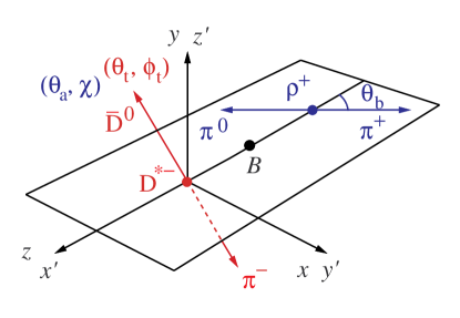
Figure 2: Angles often used for the transversity basis are shown for $D^{*}\rho$ final state.

Note, however, that one could also use the angles $(\chi,\theta_{a},\theta_{b})$ for the transversity basis.

1.3.1 $B\rightarrow\bar{D}^{*}\rho^{+}$ (helicity)

A full angular analysis of this mode has been presented at conferences [4], but has not been published. Here, we consider the decay $B\to\bar{D}^{*}\rho^{+}$ which is followed by

$$\bar{D}^{*}\to\bar{D}\pi\,,\quad\rho^{+}\to\pi^{+}\pi^{0}\,.$$ (25)

We assign,

$$a=\bar{D}^{*}\,,\quad a_{1}=\bar{D}\,,\quad a_{2}=\pi\,,\quad b=\rho^{+}\,,\quad b_{1}=\pi^{+}\,,\quad b_{2}=\pi^{0}\,.$$ (26)

The decays of $D^{*}$ and $\rho$ have only one helicity state:

$$\lambda_{a_{1}}-\lambda_{a_{2}}=0\,,\quad\lambda_{b_{1}}-\lambda_{b_{2}}=0\,.$$ (27)

Thus, the general amplitude form (17) becomes

$$A=\sum_{m}H_{m}\;e^{im\chi}d^{1}_{m,0}(\theta)d^{1}_{m,0}(\psi)\,,$$ (28)

where we have relabeled the polar angles

$$\theta=\theta_{a}\;(D^{*})\,,\quad\psi=\theta_{b}\;(\rho)\,.$$ (29)

This can be rewritten as

$$A=H_{+}g_{+}+H_{0}g_{0}+H_{-1}g_{-1}$$ (30)

where

$$g_{+1} = {1\over 2}e^{i\chi}\sin\theta\sin\psi$$

$$g_{0} = \cos\theta\cos\psi$$

$$g_{-1} = {1\over 2}e^{-i\chi}\sin\theta\sin\psi.$$ (31)

We have used

$$d^{1}_{1,1}(\theta)={1+\cos\theta\over 2}\,,\quad d^{1}_{1,0}(\theta)=-{\sin\theta\over\sqrt{2}}\,,\quad d^{1}_{1,-1}(\theta)={1-\cos\theta\over 2}\,,$$ (32)

together with

$$d^{j}_{m,m^{\prime}}(\theta)=(-)^{m-m^{\prime}}d^{j}_{m^{\prime},m}(\theta)=d^{j}_{-m^{\prime},-m}(\theta)\,.$$ (33)

The square of the amplitude is

$$|A|^{2} = (\sum_{m}H_{m}\,g_{m})^{*}(\sum_{n}H_{n}g_{n})$$ (34)

$$= \sum_{m}|H_{m}|^{2}|g_{m}|^{2}$$

$$+2\sum_{m<n}\Big{(}\Re(H_{m}^{*}H_{n})\,\Re(g^{*}_{m}g_{n})-\Im(H_{m}^{*}H_{n})\,\Im(g^{*}_{m}g_{n})\Big{)}\,.$$

Using the explicit forms for $g_{m}$, the final distribution is

$$\Gamma(\chi,\theta,\psi) = {9\over 32\pi}\Big{[}(|H_{+}|^{2}+|H_{-}|^{2})\sin^{2}\theta\sin^{2}\psi+4|H_{0}|^{2}\cos^{2}\theta\cos^{2}\psi$$ (35)

$$+2\Big{\{}\Re(H_{+}H_{-}^{*})\cos{2\chi}-\Im(H_{+}H_{-}^{*})\sin{2\chi}\Big{\}}\sin^{2}\theta\sin^{2}\psi$$

$$+\Big{\{}\Re((H_{+}+H_{-})H_{0}^{*})\cos\chi-\Im((H_{+}-H_{-})H_{0}^{*})\sin\chi\Big{\}}\sin{2\theta}\sin{2\psi}\Big{]}\,,$$

where the normalization factor is chosen such that

$$\int_{0}^{2\pi}d\chi\int_{-1}^{1}d\cos\theta\int_{-1}^{1}d\cos\psi\;\Gamma(\chi,\theta,\psi)=|H_{+}|^{2}+|H_{-}|^{2}+|H_{0}|^{2}\,.$$ (36)

1.3.2 $B\rightarrow D^{*}\rho$ (transversity)

Here, we can transform the $D^{*}$ side to transversity angles, or we could choose the $\rho$ side. We arbitrarily choose $D^{*}$ side. We start from the amplitude (30) and apply the transformations (22) and (24). We obtain

$$\begin{array}[]{llll}g_{\|}&={1\over\sqrt{2}}(g_{+}+g_{-})&={1\over\sqrt{2}}\cos\chi\sin\theta\sin\psi&={1\over\sqrt{2}}\sin\theta_{tr}\sin\phi_{tr}\sin\psi\\ g_{0}&&=\cos\theta\cos\psi&=\sin\theta_{tr}\cos\phi_{tr}\cos\psi\\ g_{\bot}&={1\over\sqrt{2}}(g_{+}-g_{-})&={i\over\sqrt{2}}\sin\chi\sin\theta\sin\psi&={i\over\sqrt{2}}\cos\theta_{tr}\sin\psi\end{array}\,,$$ (37)

to be used in

$$A(\phi_{tr},\theta_{tr},\psi)=\sum_{m}A_{m}\,g_{m}(\phi_{tr},\theta_{tr},\psi)\quad(m={\scriptstyle\|},0,\bot)\,.$$ (38)

Squaring this as before, the angular distribution becomes

$${d^{3}\Gamma(\phi_{tr},\theta_{tr},\psi)\over d\phi_{tr}d\cos\theta_{tr}d\cos\psi} = {9\over 32\pi}\bigg{(}|A_{\|}|^{2}2\sin^{2}\theta_{tr}\sin^{2}\phi_{tr}\sin^{2}\psi$$ (39)

$$+|A_{\bot}|^{2}2\cos^{2}\theta_{tr}\sin^{2}\psi+|A_{0}|^{2}4\sin^{2}\theta_{tr}\cos^{2}\phi_{tr}\cos^{2}\psi$$

$$+\sqrt{2}\Re(A_{\|}^{*}A_{0})\sin^{2}\theta_{tr}\sin{2\phi_{tr}}\sin{2\psi}-\sqrt{2}\Im(A_{0}^{*}A_{\bot})\sin{2\theta_{tr}}\cos\phi_{tr}\sin{2\psi}$$

$$-2\Im(A_{\|}^{*}A_{\bot})\sin{2\theta_{tr}}\sin\phi_{tr}\sin^{2}\psi\bigg{)}$$

Integrating this over $\phi_{tr}$ loses all interference effects among different polarization states:

$${d^{2}\Gamma(\phi_{tr},\theta_{tr},\psi)\over d\cos\theta_{tr}d\cos\psi}={9\over 16}\bigg{(}|A_{\|}|^{2}\sin^{2}\theta_{tr}\sin^{2}\psi+|A_{0}|^{2}2\sin^{2}\theta_{tr}\cos^{2}\psi+|A_{\bot}^{2}|2\cos^{2}\theta_{tr}\sin^{2}\psi\bigg{)}\,.$$ (40)

At this point, we see that the even parity states ($A_{\|}$ and $A_{0}$) have $\sin^{2}\theta_{tr}$ distribution, and the odd parity state ($A_{\bot}$) has $\cos^{2}\theta_{tr}$ distribution. Thus, plotting $\theta_{tr}$ distribution only can separate even and odd parity components. On the other hand, both $A_{\|}$ and $A_{\bot}$ are associated with $\sin^{2}\psi$, and thus $\psi$ distribution alone cannot separate different parity components. Further integrating over $\psi$ gives

$${d\Gamma(\phi_{tr},\theta_{tr},\psi)\over d\cos\theta_{tr}}={3\over 4}\bigg{(}(|A_{\|}|^{2}+|A_{0}|^{2})\sin^{2}\theta_{tr}+|A_{\bot}^{2}|2\cos^{2}\theta_{tr}\bigg{)}\,.$$ (41)

1.3.3 $B\to\Psi K^{*}$ (helicity)

The time-independent analysis has been performed by many experiments [5]. We assign

$$a=\Psi\,,\quad a_{1}=\ell^{+}\,,\quad a_{2}=\ell^{-}\,,\quad b=K^{*}\,,\quad b_{1}=K\,,\quad a_{2}=\pi\,.\quad$$ (42)

The decay $K^{*}\to K\pi$ has only one helicity state $\lambda_{b_{1,2}}=0$. On the other hand, the final state of $\Psi\to\ell^{+}\ell^{-}$ can have multiple helicity states because of the lepton spins. The actual helicity states, however, are restricted to only two due to the vector nature of the coupling that creates the lepton pair:

$$(\lambda_{\ell^{+}},\lambda_{\ell^{-}})=\Big{(}+{1\over 2},-{1\over 2}\Big{)}\;\hbox{ or }\;\Big{(}-{1\over 2},+{1\over 2}\Big{)}\,.$$ (43)

We have thus,

$$\lambda_{a_{1}}-\lambda_{a_{2}}=\pm 1\,,\quad\lambda_{b_{1}}-\lambda_{b_{2}}=0\,.$$ (44)

The final angular distribution is given by incoherent sum of the distributions for the two lepton helicity combinations:

$$\Gamma(\chi,\theta,\psi)=|A^{(+1)}|^{2}+|A^{(-1)}|^{2}\,,$$ (45)

with

$$A^{(\lambda)}=\sum_{m}H_{m}\;e^{im\chi}d^{1}_{m\lambda}(\theta)d^{1}_{m0}(\psi)\,,$$ (46)

where we have relabeled the polar angles

$$\theta=\theta_{a}\;(\Psi)\,,\quad\psi=\theta_{b}\;(K^{*})\,.$$ (47)

The amplitude (46) has the form

$$A^{(\lambda)}=\sum_{m}H_{m}\,g^{(\lambda)}_{m}\,,$$ (48)

where

$$\begin{array}[]{rcl}g^{(+1)}_{+1}&=&-{1\over 2\sqrt{2}}(1+\cos\theta)e^{i\chi}\sin\psi\\ g^{(+1)}_{0}&=&{1\over\sqrt{2}}\sin\theta\cos\psi\\ g^{(+1)}_{-1}&=&{1\over 2\sqrt{2}}(1-\cos\theta)e^{-i\chi}\sin\psi\end{array}\,,\quad\begin{array}[]{rc@{\dspl}l}g^{(-1)}_{+1}&=\hfil\displaystyle&-{1\over 2\sqrt{2}}(1-\cos\theta)e^{i\chi}\sin\psi\\ g^{(-1)}_{0}&=\hfil\displaystyle&-{1\over\sqrt{2}}\sin\theta\cos\psi\\ g^{(-1)}_{-1}&=\hfil\displaystyle&{1\over 2\sqrt{2}}(1+\cos\theta)e^{-i\chi}\sin\psi\end{array}\,.$$ (49)

The square of the amplitude (48) is

$$|A^{(\lambda)}|^{2} = (\sum_{m}H_{m}\,g^{(\lambda)}_{m})^{*}(\sum_{n}H_{,}g^{(\lambda)}_{n})$$ (50)

$$= \sum_{m}|H_{m}|^{2}|g^{(\lambda)}_{m}|^{2}$$

$$+2\sum_{m<n}\Big{(}\Re(H_{m}^{*}H_{n})\,\Re(g^{(\lambda)*}_{m}g^{(\lambda)}_{n})-\Im(H_{m}^{*}H_{n})\,\Im(g^{(\lambda)*}_{m}g^{(\lambda)}_{n})\Big{)}\,.$$

Using the explicit forms for $g^{(\lambda)}_{m}$, the final distribution is

$$\Gamma(\chi,\theta,\psi) = {9\over 64\pi}\Big{[}(|H_{+}|^{2}+|H_{-}|^{2})(1+\cos\theta^{2})\sin^{2}\psi+|H_{0}|^{2}\,4\sin^{2}\theta\cos^{2}\psi$$ (51)

$$-2\Big{\{}\Re(H_{+}^{*}H_{-})\cos{2\chi}+\Im(H_{+}^{*}H_{-})\sin{2\chi}\Big{\}}\sin^{2}\theta\sin^{2}\psi$$

$$-\Big{\{}\Re((H_{+}+H_{-})^{*}H_{0})\cos\chi+\Im((H_{+}-H_{-})^{*}H_{0})\sin\chi\Big{\}}\sin{2\theta}\sin{2\psi}\Big{]}\,,$$

where the normalization factor is chosen such that

$$\int_{0}^{2\pi}d\chi\int_{-1}^{1}d\cos\theta\int_{-1}^{1}d\cos\psi\;\Gamma(\chi,\theta,\psi)=|H_{+}|^{2}+|H_{-}|^{2}+|H_{0}|^{2}\,.$$ (52)

1.3.4 $B\to\Psi K^{*}$ (transversity)

One can use the relations (22) and (24) directly in the angular distribution (51) to obtain

$$\Gamma(\phi_{tr},\theta_{tr},\psi) = {9\over 32\pi}\Big{[}|A_{\|}|^{2}(1-\sin^{2}\theta_{tr}\sin^{2}\phi_{tr})\sin^{2}\psi$$ (53)

$$+|A_{0}|^{2}2(1-\sin^{2}\theta_{tr}\cos^{2}\phi_{tr})\cos^{2}\psi+|A_{\bot}|^{2}\sin\theta_{tr}^{2}\sin\psi^{2}$$

$$-\Re(A_{\|}^{*}A_{0}){1\over\sqrt{2}}\sin\theta_{tr}^{2}\sin{2\phi_{tr}}\sin{2\psi}+\Im(A_{0}^{*}A_{\bot}){1\over\sqrt{2}}\sin{2\theta_{tr}}\cos\phi_{tr}\sin{2\psi}$$

$$+\Im(A_{\|}^{*}A_{\bot})\sin{2\theta_{tr}}\sin\phi_{tr}\sin^{2}\psi\Big{]}\,,$$

which is normalized as

$$\int_{0}^{2\pi}d\phi_{tr}\int_{-1}^{1}d\cos\theta_{tr}\int_{-1}^{1}d\cos\psi\;\Gamma(\phi_{tr},\theta_{tr},\psi)=|A_{\|}|^{2}+|A_{\bot}|^{2}+|A_{0}|^{2}\,.$$ (54)

The transformation of angles can also be done at amplitude level. With the substitution of ampltudes (22), the amplitude for a given lepton total helicity $\lambda$ becomes

$$A^{(\lambda)}=\sum_{m}A_{m}\,g^{(\lambda)}_{m}\,,\quad(m={\scriptstyle\|},0,\bot)\,,$$ (55)

with

$$\begin{array}[]{rcl}g^{(+1)}_{\|}&=&-{1\over 2}(\cos\chi\cos\theta+i\sin\chi)\sin\psi\\ g^{(+1)}_{0}&=&{1\over\sqrt{2}}\sin\theta\cos\psi\\ g^{(+1)}_{\bot}&=&-{1\over 2}(\cos\chi+i\cos\theta\sin\chi)\sin\psi\end{array}\,,$$ (56)

$$\begin{array}[]{rc@{\dspl}l}g^{(-1)}_{\|}&=\hfil\displaystyle&{1\over 2}(\cos\chi\cos\theta-i\sin\chi)\sin\psi\\ g^{(-1)}_{0}&=\hfil\displaystyle&-{1\over\sqrt{2}}\sin\theta\cos\psi\\ g^{(-1)}_{\bot}&=\hfil\displaystyle&-{1\over 2}(\cos\chi-i\cos\theta\sin\chi)\sin\psi\end{array}\,.$$ (57)

In order to apply the transformation from $(\theta,\chi)$ to $(\theta_{tr},\phi_{tr})$, it is easier to multiply an overall phase factor which does not affect the final angular distribution. We take

$$\xi^{(+1)} = {-\cos\chi+i\cos\theta\sin\chi\over\sin\theta_{tr}}\quad{\rm for}\quad g^{(+1)}_{m}\,,$$

$$\xi^{(-1)} = {\cos\chi+i\cos\theta\sin\chi\over\sin\theta_{tr}}\quad{\rm for}\quad g^{(-1)}_{m}\,.$$ (58)

It is easy to see that these factors are indeed pure phases using the relations (24):

$$\sin^{2}\theta_{tr} = \underbrace{\sin^{2}\theta_{tr}\cos^{2}\phi_{tr}}_{\displaystyle\cos^{2}\theta}+\underbrace{\sin^{2}\theta_{tr}\sin^{2}\phi_{tr}}_{\displaystyle\sin^{2}\theta\cos^{2}\chi}=\cos\theta^{2}+\underbrace{\sin^{2}\theta\cos^{2}\chi}_{\displaystyle(1-\cos^{2}\theta)(1-\sin^{2}\chi)}$$ (59)

$$= 1-\sin^{2}\chi+\cos^{2}\theta\sin^{2}\chi=\cos^{2}\chi+\cos^{2}\theta\sin^{2}\chi\,,$$

$$\to\quad\left|{-\cos\chi+i\cos\theta\sin\chi\over\sin\theta_{tr}}\right|^{2}=\left|{\cos\chi+i\cos\theta\sin\chi\over\sin\theta_{tr}}\right|^{2}=1\,.$$ (60)

Multiplying $\xi^{(+1)}$ to $g^{(+1)}_{\|}$, we have

$$g^{(+1)}_{\|}\to g^{(+1)}_{\|}\xi^{(+1)}=-{1\over 2}(\cos\chi\cos\theta+i\sin\chi)\sin\psi{-\cos\chi+i\cos\theta\sin\chi\over\sin\theta_{tr}}\,.$$ (61)

Using

$$(\cos\chi\cos\theta+i\sin\chi)(-\cos\chi+i\cos\theta\sin\chi) = -\cos\theta-i\sin\theta^{2}\sin\chi\cos\chi$$ (62)

$$=-\sin\theta_{tr}(\cos\phi_{tr}+i\cos\theta_{tr}\sin\phi_{tr})\,,$$

the phase-rotated $g^{(+1)}_{\|}$ is then

$$g^{(+1)}_{\|}={1\over 2}(\cos\phi_{tr}+i\cos\theta_{tr}\sin\phi_{tr})\sin\psi\,.$$ (63)

Other functions are similarly obtained:

$$\begin{array}[]{rcl}g^{(+1)}_{\|}&=&{1\over 2}(\cos\phi_{tr}+i\cos\theta_{tr}\sin\phi_{tr})\sin\psi\\ g^{(+1)}_{0}&=&{1\over\sqrt{2}}(-\sin\phi_{tr}+i\cos\theta_{tr}\cos\phi_{tr})\cos\psi\\ g^{(+1)}_{\bot}&=&{1\over 2}\sin\theta_{tr}\sin\psi\end{array}\,,$$ (64)

$$\begin{array}[]{rc@{\dspl}l}g^{(-1)}_{\|}&=\hfil\displaystyle&{1\over 2}(\cos\phi_{tr}-i\cos\theta_{tr}\sin\phi_{tr})\sin\psi\\ g^{(-1)}_{0}&=\hfil\displaystyle&{1\over\sqrt{2}}(-\sin\phi_{tr}-i\cos\theta_{tr}\cos\phi_{tr})\cos\psi\\ g^{(-1)}_{\bot}&=\hfil\displaystyle&-{1\over 2}\sin\theta_{tr}\sin\psi\end{array}\,.$$ (65)

These functions gives

$$\begin{array}[]{@{\tbst}c}\vrule width=0.0pt,height=15.0pt,depth=10.0pt\lx@intercol\hfil\sum_{\lambda}|g^{(\lambda)}_{\|}|^{2}={1\over 2}(1-\sin^{2}\theta_{tr}\sin^{2}\phi_{tr})\sin^{2}\psi\,,\\ \vrule width=0.0pt,height=15.0pt,depth=10.0pt\lx@intercol\hfil\sum_{\lambda}|g^{(\lambda)}_{0}|^{2}=(1-\sin^{2}\theta_{tr}\cos^{2}\phi_{tr})\cos^{2}\psi\,,\quad\sum_{\lambda}|g^{(\lambda)}_{\bot}|^{2}={1\over 2}\sin^{2}\theta_{tr}\sin^{2}\psi\,,\\ \vrule width=0.0pt,height=15.0pt,depth=10.0pt\lx@intercol\hfil\sum_{\lambda}\Re(g^{(\lambda)*}_{\|}g^{(\lambda)}_{0})=-{1\over 4\sqrt{2}}\sin^{2}\theta_{tr}\sin{2\phi_{tr}}\sin{2\psi}\,,\quad\sum_{\lambda}\Im(g^{(\lambda)*}_{\|}g^{(\lambda)}_{0})=0\,,\\ \vrule width=0.0pt,height=15.0pt,depth=10.0pt\lx@intercol\hfil\sum_{\lambda}\Re(g^{(\lambda)*}_{\bot}g^{(\lambda)}_{0})=0\,,\quad\sum_{\lambda}\Im(g^{(\lambda)*}_{\bot}g^{(\lambda)}_{0})={1\over 4\sqrt{2}}\sin{2\theta_{tr}}\cos\phi_{tr}\sin{2\psi}\\ \vrule width=0.0pt,height=15.0pt,depth=10.0pt\lx@intercol\hfil\sum_{\lambda}\Re(g^{(\lambda)*}_{\|}g^{(\lambda)}_{\bot})=0\,,\quad\sum_{\lambda}\Im(g^{(\lambda)*}_{\|}g^{(\lambda)}_{\bot})=-{1\over 4}\sin{2\theta_{tr}}\sin\phi_{tr}\sin^{2}\psi\,,\end{array}$$ (66)

which immediately leads to (53) through (50) where $H_{m}$ are relaced by $A_{m}$. Note that three of the combinations are zero; this arises from cancellations between the two lepton helicities $\lambda=\pm 1$.

1.4 Charge conjugate decays

For the charge conjugate decays ($\bar{B}$ decays), the rule for the definitions of angles is to start from the corresponding $B$ decay, exchange paritcles and antiparticles, and then apply the definition of angles as if the daughter particles were the original particles from the $B$ decay. For example, for the decays corresponding to assignment (26) for $B\to\bar{D}^{*}\rho^{+}$, the particles in the decay $\bar{B}\to D^{*}\rho^{-}$ are assined as

$$a=D^{*}\,,\quad a_{1}=D\,,\quad a_{2}=\pi\,,\quad b=\rho^{-}\,,\quad b_{1}=\pi^{-}\,,\quad b_{2}=\pi^{0}\,.$$ (67)

and the angles $(\theta,\chi,\psi)$ are defined in the same way in terms of $a_{1,2}$ and $b_{1,2}$. In particular, the angle $\chi$ is the azimuthal angle from $b_{1}$ to $a_{1}$ measured counter-clock-wise looking down from the $a$ side.

With this definition, the angular distribution is given by (17) with replacement

$$H_{\lambda}\to\bar{H}_{\lambda}\,,$$ (68)

with

$$\bar{H}_{\lambda}\equiv\langle\bar{f}_{\lambda}|H_{\rm eff}|\bar{B}\rangle\,.$$ (69)

When $CP$ is conserved in decay, then we can take (see Appendix)

$$\bar{H}_{\lambda}=H_{-\lambda}\quad(CP)\,,$$ (70)

which holds to all orders in perturbation theory. In the literature, one sometimes encounters a $CPT$ relation $\bar{H}_{\lambda}=H_{-\lambda}^{*}$ which is correct only to first order in perturbation theory. This $CPT$ relation is thus not applicable to the decays of concern where the strong phases play inmportant role, since those phases are higher order effects. In terms of tranversity amplitudes, the $CP$ relation (68) reads

$$\bar{A}_{\|}=A_{\|}\,,\quad\bar{A}_{\bot}=-A_{\bot}\,,\quad\bar{A}_{0}=A_{0}\,.\quad(CP)$$ (71)

Inspecting the expressions for the angular distribution, one notes that moving from $B$ decay to $\bar{B}$ decay according to (70) or (71) corresponds to changing $\chi$ to $-\chi$ for the helicity formulation, and $\theta_{tr}\to\pi-\theta_{tr}$ for the transversity formulation. These are nothing but the parity transformation (or equivalantly the mirror inversion) of the configuration. Namely, if one exchanges particles and antiparticles and take mirror inversion, then the resulting angular distribution is the correct one, which is to say that $CP$ is conserved.

2 Time-dependence

In this section, we will develop a formalism suited for neutral $B$ decays to final states that are not $CP$ eigenstates. In later sections, it will be applied to $D^{*+}\pi^{-}$ final state as well as each of the three polarization states of $D^{*+}\rho^{-}$ or $\Psi K^{*}$.

First, let us recall the time evolution of pure $B^{0}$ and $\bar{B}^{0}$ states. Assuming $CPT$, the physical states $B_{a}$ and $B_{b}$ can be written as

$$\begin{array}[]{rll}B_{a}&=pB^{0}+q\bar{B}^{0}&\quad(m_{a},\gamma_{a})\\ B_{b}&=pB^{0}-q\bar{B}^{0}&\quad(m_{b},\gamma_{b})\end{array}\,,$$ (72)

where $m_{a,b}$ and $\gamma_{a,b}$ are the masses and decay rates of the corresponding physical states. Theoretically and experimentally, $|p|=|q|$ within error of order 1%. Here, we assume $|p|=|q|$ which makes $p/q$ a pure phase factor. The lowest order estimation gives (see Appendix)

$${p\over q}=-{V_{td}^{*}V_{tb}\over V_{td}V_{tb}^{*}}\,.$$ (73)

which corresponds to the choice of the $CP$ phase of the neutral $B$ meson given by

$$CP|B^{0}\rangle=\eta_{B}|\bar{B}^{0}\rangle\,,\quad CP|\bar{B}^{0}\rangle=\eta_{B}^{*}|B^{0}\rangle\,,\quad{\rm with}\quad\eta_{B}=1.$$ (74)

The above value of $p/q$ is for the case $B_{a}$ is heavier than $B_{b}$:

$$m_{a}>m_{b}\,.$$ (75)

The physical states evolve as

$$B_{a}\to B_{a}e^{-im_{a}t-{\gamma_{a}\over 2}t}\,,\quad B_{b}\to B_{b}e^{-im_{b}t-{\gamma_{b}\over 2}t}\,.$$ (76)

Hereafter, we will assume that the decay rates of the two physical states are the same

$$\gamma_{a}=\gamma_{b}\equiv\gamma\,.$$ (77)

then, the factor $e^{-{\gamma\over 2}t}$ decouples from all amplitudes, which we will drop for now and restore it at the end. We also separate an overall phase factor $\exp(-i{m_{a}+m_{b}\over 2}t)$ and discard it since such overall phase factors do not affect measurable quantities. Then the evolutions of $B_{a,b}$ can be simplified as

$$B_{a}\to B_{a}e^{-i{\delta m\over 2}t}\,,\quad B_{b}\to B_{b}e^{i{\delta m\over 2}t}\,\qquad(\times e^{-{\gamma\over 2}t})\,,$$ (78)

with

$$\delta m\equiv m_{a}-m_{b}>0\,.$$ (79)

Then, the time evolutions of pure $B^{0}$ and $\bar{B}^{0}$ can be obtained by solving (72) for $B^{0}$ and $\bar{B}^{0}$ and then applying the time evolutions above:

$$B^{0}={B_{a}+B_{b}\over 2p}\to{1\over 2p}(\underbrace{B_{a}}_{\displaystyle pB^{0}+q\bar{B}^{0}}e^{-i{\delta m\over 2}t}+\underbrace{B_{b}}_{\displaystyle pB^{0}-q\bar{B}^{0}}e^{i{\delta m\over 2}t})=B^{0}\cos{\delta mt\over 2}-{q\over p}\bar{B}^{0}i\sin{\delta mt\over 2}\,.$$ (80)

The time evolution of $\bar{B}$ is similarly obtained. Restoring the decay factor $e^{-{\gamma\over 2}t}$,

$$B^{0} \to e^{-{\gamma\over 2}t}\left(B^{0}\cos{\delta m\,t\over 2}-{q\over p}\bar{B}^{0}i\sin{\delta m\,t\over 2}\right)\,,$$

$$\bar{B}^{0} \to e^{-{\gamma\over 2}t}\left(\bar{B}^{0}\cos{\delta m\,t\over 2}-{p\over q}B^{0}i\sin{\delta m\,t\over 2}\right)\,.$$ (81)

We now consider the decay amplitudes for a pure $B^{0}$ or $\bar{B}^{0}$ state at $t=0$ to decay to a final state $f$ or its charge conjugate state $\bar{f}$ at time $t$. The final state could be $D^{(*)-}\pi^{+}$ or any given polarization state of $D^{*-}\rho^{+}$ or $\Psi K^{*0}$. Define four instantaneous dedcay amplitudes by

$$\begin{array}[]{rcl}a&\equiv&Amp(B^{0}\to f)\\ \bar{a}&\equiv&Amp(\bar{B}^{0}\to\bar{f})\\ b&\equiv&Amp(B^{0}\to\bar{f})\\ \bar{b}&\equiv&Amp(\bar{B}^{0}\to f)\end{array}\,,$$ (82)

For $f=D^{(*)-}\pi^{+}$, for example, $a$ and $\bar{a}$ are the favored amplitudes and $b$ and $\bar{b}$ are the suppressed amplitudes. Then, (81) gives

$$\begin{array}[]{rcl@{\tbst}l}A_{B^{0}\to f}(t)&=&e^{-{\gamma\over 2}t}\left(a\cos{\delta m\,t\over 2}-{q\over p}\bar{b}\,i\sin{\delta m\,t\over 2}\right)\hfil\vrule width=0.0pt,height=15.0pt,depth=10.0pt&=e^{-{\gamma\over 2}t}a\left(\cos{\delta m\,t\over 2}-\rho\,i\sin{\delta m\,t\over 2}\right)\\ A_{\bar{B}^{0}\to\bar{f}}(t)&=&e^{-{\gamma\over 2}t}\left(\bar{a}\cos{\delta m\,t\over 2}-{p\over q}b\,i\sin{\delta m\,t\over 2}\right)\hfil\vrule width=0.0pt,height=15.0pt,depth=10.0pt&=e^{-{\gamma\over 2}t}\bar{a}\left(\cos{\delta m\,t\over 2}-\bar{\rho}\,i\sin{\delta m\,t\over 2}\right)\\ A_{B^{0}\to\bar{f}}(t)&=&e^{-{\gamma\over 2}t}\left(b\cos{\delta m\,t\over 2}-{q\over p}\bar{a}\,i\sin{\delta m\,t\over 2}\right)\hfil\vrule width=0.0pt,height=15.0pt,depth=10.0pt&=e^{-{\gamma\over 2}t}\bar{a}\left(\bar{\rho}\cos{\delta m\,t\over 2}-i\sin{\delta m\,t\over 2}\right)\\ A_{\bar{B}^{0}\to f}(t)&=&e^{-{\gamma\over 2}t}\left(\bar{b}\cos{\delta m\,t\over 2}-{p\over q}a\,i\sin{\delta m\,t\over 2}\right)\hfil\vrule width=0.0pt,height=15.0pt,depth=10.0pt&=e^{-{\gamma\over 2}t}a\left(\rho\cos{\delta m\,t\over 2}-i\sin{\delta m\,t\over 2}\right)\end{array}$$ (83)

with

$$\rho\equiv{q\,\bar{b}\over p\,a}\,,\quad\bar{\rho}\equiv{p\,b\over q\,\bar{a}}\,.$$ (84)

For the bottom two amplitudes (the ‘suppressed’ decays), we have ignored overall phase factors $p/q$ and $q/p$ for the second equalities.

At this point, we can see the relation between the ‘suppressed’ and ‘favored’ modes; namely, up to an overall phase, $\delta mt\to\delta mt+\pi$ transforms $A_{B^{0}\to f}(t)$ to $A_{\bar{B}^{0}\to f}(t)$ and $A_{B^{0}\to f}(t)$ to $A_{\bar{B}^{0}\to f}(t)$. Equivalently, in the expressions of decay rates,

$$(\cos\delta mt,\sin\delta mt)\leftrightarrow(-\cos\delta mt,-\sin\delta mt)$$ (85)

transforms between a suppressed mode and its favoed mode with the same final state. Also, $p/q$ is the complex conjugate of $q/p$ (within the approximation that $|p|=|q|$), and as we will see more explicity later, the weak phase of $b/\bar{a}$ is the complex conjugate of that of $\bar{b}/a$ with the rest being the ‘strong phase’ which is common to both. Thus,

$$(\hbox{weak phase})\leftrightarrow-(\hbox{weak phase})$$ (86)

keeping the strong phase the same transforms between a $B^{0}$ decay and the corresponding $\bar{B}^{0}$ decay (both ‘suppressed’ or both ‘favored’) apart from the difference between $a$ and $\bar{a}$. Often $|a|$ and $|\bar{a}|$ are the same and if so the above transformation is exact in the decay rates. When we extend the above time-dependent amplitudes to include interferences between polarizations, the rule between the same final state (85) still holds, but the relation between $B^{0}$ and $\bar{B}^{0}$ (86) does not hold in the helicity basis. We will see, however, that it holds in the transversity basis.

The time dependent rates are obtained by squaring (83):

$$\begin{array}[]{rc@{\tbst}l}\Gamma_{B^{0}\to f}(t)&=\hfil\vrule width=0.0pt,height=15.0pt,depth=10.0pt&|a|^{2}{e^{-\gamma t}\over 2}\left[(1+|\rho|^{2})+(1-|\rho|^{2})\cos\delta mt+2\Im\rho\,\sin\delta mt\right]\\ \Gamma_{\bar{B}^{0}\to\bar{f}}(t)&=\hfil\vrule width=0.0pt,height=15.0pt,depth=10.0pt&|\bar{a}|^{2}{e^{-\gamma t}\over 2}\left[(1+|\bar{\rho}|^{2})+(1-|\bar{\rho}|^{2})\cos\delta mt+2\Im\bar{\rho}\,\sin\delta mt\right]\\ \Gamma_{B^{0}\to f}(t)&=\hfil\vrule width=0.0pt,height=15.0pt,depth=10.0pt&|\bar{a}|^{2}{e^{-\gamma t}\over 2}\left[(1+|\bar{\rho}|^{2})-(1-|\bar{\rho}|^{2})\cos\delta mt-2\Im\bar{\rho}\,\sin\delta mt\right]\\ \Gamma_{\bar{B}^{0}\to f}(t)&=\hfil\vrule width=0.0pt,height=15.0pt,depth=10.0pt&|a|^{2}{e^{-\gamma t}\over 2}\left[(1+|\rho|^{2})-(1-|\rho|^{2})\cos\delta mt-2\Im\rho\,\sin\delta mt\right]\end{array}\,.$$ (87)

In deriving this formula, we have assumed $CPT$ in the mixing and that $\gamma_{a}=\gamma_{b}$. Otherwise, it is general; in particular, there could be direct $CP$ violations in any of the decay amplitudes such as $|a|\not=|\bar{a}|$ etc.

On $\Upsilon(4S)$, one would flavor-tag the other side by, say, a lepton. If the tag side decays to $\ell^{-}$ at proper time $t_{tag}$, the quantum correlation is such that the signal side is pure $B^{0}$ at the same proper time $t_{sig}=t_{tag}$ and proceed to evolve as usual from that time on. Thus, for $t_{sig}>t_{tag}$, the decay distribution is given simply by the replacement

$$t\to\Delta t\equiv t_{sig}-t_{tag}\,.$$ (88)

For $t_{sig}<t_{tag}$, all that is needed is to put absolute value on $\Delta t$ of the decay factor $e^{-\gamma\Delta t}$. Namely, (87) becomes the distributions on $\Upsilon(4S)$ with the replacement

$$\gamma t\to\gamma|\Delta t|\quad{\rm and}\quad\delta mt\to\delta m\Delta t\,.$$ (89)

Explicitly,

$$\begin{array}[]{rc@{\tbst}l}\Gamma_{\ell^{-},f}(\Delta t)&=\hfil\vrule width=0.0pt,height=15.0pt,depth=10.0pt&|a|^{2}{e^{-\gamma|\Delta t|}\over 2}\left[(1+|\rho|^{2})+(1-|\rho|^{2})\cos\delta m\Delta t+2\Im\rho\,\sin\delta m\Delta t\right]\\ \Gamma_{\ell^{+},\bar{f}}(\Delta t)&=\hfil\vrule width=0.0pt,height=15.0pt,depth=10.0pt&|\bar{a}|^{2}{e^{-\gamma|\Delta t|}\over 2}\left[(1+|\bar{\rho}|^{2})+(1-|\bar{\rho}|^{2})\cos\delta m\Delta t+2\Im\bar{\rho}\,\sin\delta m\Delta t\right]\\ \Gamma_{\ell^{-},f}(\Delta t)&=\hfil\vrule width=0.0pt,height=15.0pt,depth=10.0pt&|\bar{a}|^{2}{e^{-\gamma|\Delta t|}\over 2}\left[(1+|\bar{\rho}|^{2})-(1-|\bar{\rho}|^{2})\cos\delta m\Delta t-2\Im\bar{\rho}\,\sin\delta m\Delta t\right]\\ \Gamma_{\ell^{+},f}(\Delta t)&=\hfil\vrule width=0.0pt,height=15.0pt,depth=10.0pt&|a|^{2}{e^{-\gamma|\Delta t|}\over 2}\left[(1+|\rho|^{2})-(1-|\rho|^{2})\cos\delta m\Delta t-2\Im\rho\,\sin\delta m\Delta t\right]\end{array}\,,$$ (90)

where $\Gamma_{\ell^{-},f}(\Delta t)$ denotes the decay rate for one side decaying to a final state $f$ while the opposite side is tagged by a negative lepton (or tagged as $\bar{B}^{0}$ by any other method), etc.

2.1 $B^{0}\to D^{(*)-}\pi^{+}$

Earlier studies of this mode can be found in Ref. [6]. Diagrams for $\bar{B}^{0}\to D^{\mp}\pi^{\pm}$ are shown in Figure 3.

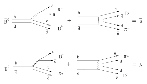
Figure 3: Diagrams for $\bar{B}^{0}\to D^{\pm}\pi^{\mp}$.

In addition to dominant tree diagrams, annihilation diagrams may have non-negligible contribution. Also, there may be final-state rescattering $\bar{D}^{(*)0}\pi^{0}\to D^{(*)-}\pi^{+}$. The $CKM$ factor of these processes, however, is the same as that of the corresponding tree diagram for the same final state, and thus it does not affect the following formulation. Penguins should result in even number of charms; thus, penguins do not contribute.

With the definitions $f\equiv D^{-}\pi^{+}$ and $\bar{f}\equiv D^{+}\pi^{-}$, the four amplitudes of (82) can be written as

$$\begin{array}[]{@{\tbst}rcl}\vrule width=0.0pt,height=15.0pt,depth=10.0pt\lx@intercol\hfil a&\equiv&Amp(B^{0}\to D^{-}\pi^{+})=\lambda_{c}^{*}F_{c}\\ \vrule width=0.0pt,height=15.0pt,depth=10.0pt\lx@intercol\hfil\bar{a}&\equiv&Amp(\bar{B}^{0}\to D^{+}\pi^{-})=\lambda_{c}\bar{F}_{c}\\ \vrule width=0.0pt,height=15.0pt,depth=10.0pt\lx@intercol\hfil b&\equiv&Amp(B^{0}\to D^{+}\pi^{-})=\lambda_{u}^{*}F_{u}\\ \vrule width=0.0pt,height=15.0pt,depth=10.0pt\lx@intercol\hfil\bar{b}&\equiv&Amp(\bar{B}^{0}\to D^{-}\pi^{+})=\lambda_{u}\bar{F}_{u}\end{array}\quad{\rm with}\quad\begin{array}[]{rcl}\lambda_{c}\equiv V_{cb}V_{ud}^{*}\\ \lambda_{u}\equiv V_{ub}V_{cd}^{*}\end{array}\,,$$ (91)

where we have separated the $CKM$ factors $\lambda_{c,u}^{(*)}$ and called the rest $F_{c,u}$ which include strong phases as well as decay constants and form factors (if factorization is assumed). We assume that the $CP$ violation is solely through the weak phases that appear in (91); as a consequence we can show that (see Appendix)

$$F_{c}=\bar{F}_{c}\,,\quad F_{u}=\bar{F}_{u}\,.$$ (92)

We then have

$$|a|=|\bar{a}|\,,\quad|b|=|\bar{b}|\,.$$ (93)

Using (73) and (82) as well as (92), the value of $\bar{\rho}$ defined in (84) is then

$$\bar{\rho}\equiv{p\,b\over q\,\bar{a}}={p\,\lambda_{u}^{*}F_{u}\over q\,\lambda_{c}F_{c}}=-{V_{td}^{*}V_{tb}\over V_{td}V_{tb}^{*}}{V_{ub}^{*}V_{cd}\over V_{cb}V_{ud}^{*}}{F_{u}\over F_{c}}\equiv re^{i\phi_{\bar{\rho}}}\,.$$ (94)

where we have defined $r\equiv|\bar{\rho}|$ and $\phi_{\bar{\rho}}\equiv\arg\bar{\rho}$. With the definitions of $\phi_{1}$ and $\phi_{3}$

$$\phi_{1}\equiv\arg{V_{cd}V_{cb}^{*}\over-V_{td}V_{tb}^{*}}\,,\quad\phi_{3}\equiv\arg{V_{ud}V_{ub}^{*}\over-V_{cd}V_{cb}^{*}}\,,$$ (95)

we have

$$\arg\left(-{V_{td}^{*}V_{tb}\over V_{td}V_{tb}^{*}}{V_{ub}^{*}V_{cd}\over V_{cb}V_{ud}^{*}}\right)=\arg\left({V_{cd}V_{cb}^{*}\over-V_{td}V_{tb}^{*}}{V_{cd}V_{cb}^{*}\over-V_{td}V_{tb}^{*}}{V_{ud}V_{ub}^{*}\over-V_{cd}V_{cb}^{*}}\right)=2\phi_{1}+\phi_{3}\,.$$ (96)

Then, $\bar{\rho}$ can be written as

$$\bar{\rho}=re^{i(\phi_{w}+\delta)}\,.$$ (97)

with

$$\phi_{w}\equiv 2\phi_{1}+\phi_{3}\,,\quad\delta\equiv\arg{F_{u}\over F_{c}}\,.$$ (98)

Similarly, one obtains

$$\rho=re^{-i(\phi_{w}-\delta)}\,.$$ (99)

Note that we have $|\rho|=|\bar{\rho}|=r$. The value of $r$ is roughly

$$r=\left|{V_{ub}^{*}V_{cd}\over V_{cb}V_{ud}^{*}}{F_{u}\over F_{c}}\right|\sim 0.4\lambda^{2}\sim 0.02\,.\quad(\lambda\sim 0.22:\hbox{Cabibbo factor})\,.$$ (100)

With $\Im\rho=-r\sin(\phi_{w}-\delta)$ and $\Im\bar{\rho}=r\sin(\phi_{w}+\delta)$, the four decay rates (87) becomes

$$\begin{array}[]{rc@{\tbst}l}\Gamma_{B^{0}\to D^{-}\pi^{+}}(t)&=\hfil\vrule width=0.0pt,height=15.0pt,depth=10.0pt&|a|^{2}{e^{-\gamma t}\over 2}\left[(1+r^{2})+(1-r^{2})\cos\delta mt-2r\sin(\phi_{w}-\delta)\,\sin\delta mt\right]\\ \Gamma_{\bar{B}^{0}\to D^{+}\pi^{-}}(t)&=\hfil\vrule width=0.0pt,height=15.0pt,depth=10.0pt&|a|^{2}{e^{-\gamma t}\over 2}\left[(1+r^{2})+(1-r^{2})\cos\delta mt+2r\sin(\phi_{w}+\delta)\,\sin\delta mt\right]\\ \Gamma_{B^{0}\to D^{+}\pi^{-}}(t)&=\hfil\vrule width=0.0pt,height=15.0pt,depth=10.0pt&|a|^{2}{e^{-\gamma t}\over 2}\left[(1+r^{2})-(1-r^{2})\cos\delta mt-2r\sin(\phi_{w}+\delta)\,\sin\delta mt\right]\\ \Gamma_{\bar{B}^{0}\to D^{-}\pi^{+}}(t)&=\hfil\vrule width=0.0pt,height=15.0pt,depth=10.0pt&|a|^{2}{e^{-\gamma t}\over 2}\left[(1+r^{2})-(1-r^{2})\cos\delta mt+2r\sin(\phi_{w}-\delta)\,\sin\delta mt\right]\end{array}\,.$$ (101)

where have used $|a|=|\bar{a}|$. Note that $\Gamma_{\bar{B}^{0}\to D^{-}\pi^{+}}(t)$ (suppressed) is obtained from $\Gamma_{B^{0}\to D^{-}\pi^{+}}(t)$ (favored) and $\Gamma_{B^{0}\to D^{+}\pi^{-}}(t)$ (suppressed) is obtained from $\Gamma_{\bar{B}^{0}\to D^{+}\pi^{-}}(t)$ (favored) by the transformation (85), and within the two suppressed modes and within the favored modes, the expresssions are related by (86) namely $\phi_{w}\leftrightarrow-\phi_{w}$.

The $CP$ violating parameters that can be extracted from these distributions are

$$r\sin(\phi_{w}-\delta)\quad{\rm and}\quad r\sin(\phi_{w}+\delta)\,.$$ (102)

Note that the two extractable paramters are always multiplied with $r$, and the value of $r$ cannot be obtained by the fit. As discussed earlier, the corresponding distributions on $\Upsilon(4S)$ are obtained by replacements $\gamma t\to\gamma|\Delta t|$ and $\delta mt\to\delta m\Delta t$. The first paramter $r\sin(\phi_{w}-\delta)$ can be obtained through the asymmetry between positive and negative $\Delta t$ of $\Gamma_{\ell^{-},D^{-}\pi^{+}}(\Delta t)$ (favored) or $\Gamma_{\ell^{+},D^{-}\pi^{+}}(\Delta t)$ (suppressed), and the second paramter $r\sin(\phi_{w}+\delta)$ is similarly obtained through $\Gamma_{\ell^{+},D^{+}\pi^{-}}(t)$ (favored) or $\Gamma_{\ell^{-},D^{+}\pi^{-}}(t)$ (suppressed). This feature that single mode can give a $CP$ violating parameter through asymmetry between positive and negative $\Delta t$ is unique to $\Upsilon(4S)$. In fact, most of the information on $CP$ violation is in such asymmetries. If we define

$$\delta\Gamma_{X}(|\Delta t|)\equiv\Gamma_{X}(\Delta t)-\Gamma_{X}(-\Delta t)\,,$$ (103)

we have

$$-\delta\Gamma_{\ell^{-},D^{-}\pi^{+}}(|\Delta t|)=\delta\Gamma_{\ell^{+},D^{-}\pi^{+}}(|\Delta t|) = Nr\sin(\phi_{w}-\delta)e^{-\gamma t}\sin(\delta mt)\,,$$ (104)

$$\delta\Gamma_{\ell^{+},D^{+}\pi^{-}}(|\Delta t|)=-\delta\Gamma_{\ell^{-},D^{+}\pi^{-}}(|\Delta t|) = Nr\sin(\phi_{w}+\delta)e^{-\gamma t}\sin(\delta mt)\,,$$ (105)

where $N$ is a common normalization factor which is known.

Now we derive the corresponding time-integrated expressions. We use following integrals.

$$\,\int_{0}^{\infty}e^{-\gamma t}\,dt =\frac{1}{\gamma}\,,$$ (106)

$$\,\int_{0}^{\infty}e^{-\gamma t}\sin\delta mt\,dt =\frac{1}{\gamma}\frac{x}{1+x^{2}}\,,$$ (107)

$$\,\int_{0}^{\infty}e^{-\gamma t}\cos\delta mt\,dt =\frac{1}{\gamma}\frac{1}{1+x^{2}}\,.$$ (108)

Here $x={\delta m}/{\gamma}$. The time-integrated decay rates become

$$\Gamma(B^{0}\rightarrow D^{-}\pi^{+}) = \frac{|a|^{2}}{2\gamma}[(1+r^{2})+\frac{1-r^{2}}{1+x^{2}}-\frac{2rx}{1+x^{2}}\sin(\phi_{w}-\delta)]$$

$$\Gamma(\bar{B}^{0}\rightarrow D^{+}\pi^{-}) = \frac{|a|^{2}}{2\gamma}[(1+r^{2})+\frac{1-r^{2}}{1+x^{2}}+\frac{2rx}{1+x^{2}}\sin(\phi_{w}+\delta)]$$

$$\Gamma(B^{0}\rightarrow D^{+}\pi^{-}) = \frac{|a|^{2}}{2\gamma}[(1+r^{2})-\frac{1-r^{2}}{1+x^{2}}-\frac{2rx}{1+x^{2}}\sin(\phi_{w}+\delta)]$$

$$\Gamma(\bar{B}^{0}\rightarrow D^{-}\pi^{+}) = \frac{|a|^{2}}{2\gamma}[(1+r^{2})-\frac{1-r^{2}}{1+x^{2}}+\frac{2rx}{1+x^{2}}\sin(\phi_{w}-\delta)]$$ (109)

If we set $\delta=0$ for simplicity, we see that the information on $\sin(\phi_{w})$ is in the asymmetry between the top two rates (the favored modes) or in the asymmetry between the bottom two rates (the suppressed modes). The absolute amount of the differnce is the same for both cases, but the total rate is about 5 times larger for the favored modes compared to the suppressed modes. It means that the significance (number of sigmas) is $\sqrt{5}$ times smaller for the favored modes. Thus, most of the information is contained in the suppressed modes.

The expressions (101) and (109) are valid also for $f=D^{*-}\pi^{+}$, $D^{-}\rho^{+}$. When there are more than one polarization states as in $D^{*-}\rho^{+}$, there is extra effect due to interferences between different polarization states, which we will discuss next.

2.2 $B^{0}\to D^{*-}\rho^{+}$

This mode was first stdied in detail in Ref. [7]. We first note that the expressions for the time dependent amplitudes (83) are still valid when applied to each polarization state:

$$\begin{array}[]{rc@{\tbst}lrcl}A_{B^{0}\to f_{\lambda}}(t)&=\hfil\vrule width=0.0pt,height=15.0pt,depth=10.0pt&e^{-{\gamma\over 2}t}\,\left(a_{\lambda}\cos{\delta m\,t\over 2}-{q\over p}\bar{b}_{\lambda}i\sin{\delta m\,t\over 2}\right)&=&e^{-{\gamma\over 2}t}\,a_{\lambda}\left(\cos{\delta m\,t\over 2}-\rho_{\lambda}\,i\sin{\delta m\,t\over 2}\right)\\ A_{\bar{B}^{0}\to\bar{f}_{\lambda}}(t)&=\hfil\vrule width=0.0pt,height=15.0pt,depth=10.0pt&e^{-{\gamma\over 2}t}\,\left(\bar{a}_{\lambda}\cos{\delta m\,t\over 2}-{p\over q}b_{\lambda}i\sin{\delta m\,t\over 2}\right)&=&e^{-{\gamma\over 2}t}\,\bar{a}_{\lambda}\left(\cos{\delta m\,t\over 2}-\bar{\rho}_{\lambda}\,i\sin{\delta m\,t\over 2}\right)\\ A_{B^{0}\to\bar{f}_{\lambda}}(t)&=\hfil\vrule width=0.0pt,height=15.0pt,depth=10.0pt&e^{-{\gamma\over 2}t}\,\left(b_{\lambda}\cos{\delta m\,t\over 2}-{q\over p}\bar{a}_{\lambda}i\sin{\delta m\,t\over 2}\right)&=&e^{-{\gamma\over 2}t}\,\bar{a}_{\lambda}\left(\bar{\rho}_{\lambda}\cos{\delta m\,t\over 2}-i\sin{\delta m\,t\over 2}\right)\\ A_{\bar{B}^{0}\to f_{\lambda}}(t)&=\hfil\vrule width=0.0pt,height=15.0pt,depth=10.0pt&e^{-{\gamma\over 2}t}\,\left(\bar{b}_{\lambda}\cos{\delta m\,t\over 2}-{p\over q}a_{\lambda}i\sin{\delta m\,t\over 2}\right)&=&e^{-{\gamma\over 2}t}\,a_{\lambda}\left(\rho_{\lambda}\cos{\delta m\,t\over 2}-i\sin{\delta m\,t\over 2}\right)\end{array}$$ (110)

where

$$\begin{array}[]{r@{\tbst}cl}a_{\lambda}\vrule width=0.0pt,height=15.0pt,depth=10.0pt&\equiv&Amp(B^{0}\to f_{\lambda})=\lambda_{c}^{*}F_{c\lambda}\\ \bar{a}_{\lambda}\vrule width=0.0pt,height=15.0pt,depth=10.0pt&\equiv&Amp(\bar{B}^{0}\to\bar{f}_{\lambda})=\lambda_{c}\bar{F}_{c\lambda}\\ b_{\lambda}\vrule width=0.0pt,height=15.0pt,depth=10.0pt&\equiv&Amp(B^{0}\to\bar{f}_{\lambda})=\lambda_{u}^{*}F_{u\lambda}\\ \bar{b}_{\lambda}\vrule width=0.0pt,height=15.0pt,depth=10.0pt&\equiv&Amp(\bar{B}^{0}\to f_{\lambda})=\lambda_{u}\bar{F}_{u\lambda}\end{array}\,,$$ (111)

and

$$\rho_{\lambda}\equiv{q\,\bar{b}_{\lambda}\over p\,a_{\lambda}}\,,\quad\bar{\rho}_{\lambda}\equiv{p\,b_{\lambda}\over q\,\bar{a}_{\lambda}}\,.$$ (112)

Each of (110) gives the polarization amplitudes to a given final state at time $t$. Then, the angular distribution of pure $B^{0}$ at $t=0$ decaying to $f$ at time $t$ is simply obtained by replacing $H_{\lambda}$ or $A_{\lambda}$ by $A_{B^{0}\to f_{\lambda}}(t)$ in (35) or (39). For $B^{0}(t=0)\to f$, for example, the time-dependent angular distribution is given by (39) with the replacement

$$|A_{\lambda}|^{2} \to |A_{B^{0}\to f_{\lambda}}(t)|^{2}\,,$$

$$\Re(A_{\|}^{*}A_{0}) \to \Re(A^{*}_{B^{0}\to f_{\|}}(t)A_{B^{0}\to f_{0}}(t))\,,$$

$$\Im(A_{0}^{*}A_{\bot}) \to \Im(A^{*}_{B^{0}\to f_{0}}(t)A_{B^{0}\to f_{\bot}}(t))\,,$$

$$\Im(A_{\|}^{*}A_{\bot}) \to \Im(A^{*}_{B^{0}\to f_{\|}}(t)A_{B^{0}\to f_{\bot}}(t))\,.$$ (113)

Or the decay amplitudes are obtained from (38) by the same replacement:

$$A_{B^{0}\to f}(\Omega,t) = \sum_{\lambda}e^{-{\gamma\over 2}t}\,a_{\lambda}\left(\cos{\delta m\,t\over 2}-\rho_{\lambda}\,i\sin{\delta m\,t\over 2}\right)g_{\lambda}(\Omega)$$

$$A_{\bar{B}^{0}\to\bar{f}}(\Omega,t) = \sum_{\lambda}e^{-{\gamma\over 2}t}\,\bar{a}_{\lambda}\left(\cos{\delta m\,t\over 2}-\bar{\rho}_{\lambda}\,i\sin{\delta m\,t\over 2}\right)g_{\lambda}(\Omega)$$

$$A_{B^{0}\to\bar{f}}(\Omega,t) = \sum_{\lambda}e^{-{\gamma\over 2}t}\,\bar{a}_{\lambda}\left(\bar{\rho}_{\lambda}\,\cos{\delta m\,t\over 2}-i\sin{\delta m\,t\over 2}\right)g_{\lambda}(\Omega)$$

$$A_{\bar{B}^{0}\to f}(\Omega,t) = \sum_{\lambda}e^{-{\gamma\over 2}t}\,a_{\lambda}\left(\rho_{\lambda}\,\cos{\delta m\,t\over 2}-i\sin{\delta m\,t\over 2}\right)g_{\lambda}(\Omega)\,,$$ (114)

where $\Omega\equiv(\phi_{tr},\theta_{tr},\psi)$ or $(\chi,\theta,\psi)$, and $g_{\lambda}$’s are given by (37) or (31). Here, the final states are $f\equiv D^{*-}\rho^{+}$ and $\bar{f}\equiv D^{*+}\rho^{-}$. Note that one could use angles $(\phi_{tr},\theta_{tr},\psi)$ or $(\chi,\theta,\psi)$ for the tranversity amplitudes (for that matter, for the helicity amplitudes also - we just have not provided $g(\phi_{tr},\theta_{tr},\psi)$ for the helicity amplitudes).

Since $F_{u\lambda}$ and $F_{c\lambda}$ are nothing but the polarization amplitudes apart from the $CP$ violating phases, they themselves should satisfy the $CP$ relations (70) and (71) (see Appendix):

$$\bar{F}_{q\lambda}=F_{q-\lambda}\quad(\hbox{helicity})\,,$$ (115)

$$\bar{F}_{q\|}=F_{q\|}\,,\quad\bar{F}_{q0}=F_{q0}\,,\quad\bar{F}_{q\bot}=-F_{u\bot}\,,\quad(\hbox{tranversity})$$ (116)

where $q=u$ or $c$.

2.2.1 Helicity basis

With the relations (115) for helicity basis, the decay amplitudes can be written as

$$\begin{array}[]{r@{\tbst}clrcl}a_{\lambda}\vrule width=0.0pt,height=15.0pt,depth=10.0pt&=&\lambda_{c}^{*}F_{c\lambda}\,,\quad\bar{a}_{-\lambda}&=&\lambda_{c}F_{c\lambda}\,,\\ b_{\lambda}\vrule width=0.0pt,height=15.0pt,depth=10.0pt&=&\lambda_{u}^{*}F_{u\lambda}\,,\quad\bar{b}_{-\lambda}&=&\lambda_{u}F_{u\lambda}\,.\end{array}\quad(\hbox{helicity})$$ (117)

This gives

$$|a_{\lambda}|=|\bar{a}_{-\lambda}|\,,\quad|b_{\lambda}|=|\bar{b}_{-\lambda}|\,.$$ (118)

And the parameters $\rho_{\lambda}$ and $\bar{\rho}_{\lambda}$ becomes

$$\rho_{\lambda}={q\over p}{\lambda_{u}F_{u-\lambda}\over\lambda_{c}^{*}F_{c\lambda}}\,,\quad\bar{\rho}_{-\lambda}={p\over q}{\lambda_{u}^{*}F_{u-\lambda}\over\lambda_{c}F_{c\lambda}}\,.$$ (119)

Then, the same procedure that led to (97) and (99) allows one to write

$$\rho_{\lambda}=r_{\lambda}e^{i(\phi_{w}+\delta_{\lambda})}\,,\quad\bar{\rho}_{-\lambda}=r_{\lambda}e^{-i(\phi_{w}-\delta_{\lambda})}\,,\quad$$ (120)

where

$$|\rho_{\lambda}|=|\bar{\rho}_{-\lambda}|\equiv r_{\lambda}\,,$$ (121)

and

$$\delta_{\lambda}\equiv\arg{F_{u-\lambda}\over F_{c\lambda}}\,.$$ (122)

2.2.2 Transversity basis

Using the relations (116) for transversity, we can write

$$\begin{array}[]{r@{\tbst}clrcl}a_{\lambda}\vrule width=0.0pt,height=15.0pt,depth=10.0pt&=&\lambda_{c}^{*}F_{c\lambda}\,,\quad\bar{a}_{\lambda}&=&\xi_{\lambda}\lambda_{c}F_{c\lambda}\,,\\ b_{\lambda}\vrule width=0.0pt,height=15.0pt,depth=10.0pt&=&\lambda_{u}^{*}F_{u\lambda}\,,\quad\bar{b}_{\lambda}&=&\xi_{\lambda}\lambda_{u}F_{u\lambda}\,,\end{array}\quad(\hbox{transversity})$$ (123)

where

$$\xi_{\lambda}=\left\{\begin{array}[]{rl}1&\quad(\lambda={\scriptstyle\|},0)\\ -1&\quad(\lambda=\bot)\end{array}\right.\,.$$ (124)

We will use the tranveristy basis for the rest of this section. Clearly, we have

$$|a_{\lambda}|=|\bar{a}_{\lambda}|\quad{\rm and}\quad|b_{\lambda}|=|\bar{b}_{\lambda}|\,,$$ (125)

and the procedure semilar to that led to (97) and (99) gives

$$\rho_{\lambda}=\xi_{\lambda}r_{\lambda}e^{-i(\phi_{w}-\delta_{\lambda})}\,,\quad\bar{\rho}_{\lambda}=\xi_{\lambda}r_{\lambda}e^{i(\phi_{w}+\delta_{\lambda})}\,,$$ (126)

where

$$|\rho_{\lambda}|=|\bar{\rho}_{\lambda}|\equiv r_{\lambda}\,,$$ (127)

and

$$\delta_{\lambda}\equiv\arg{F_{u\lambda}\over F_{c\lambda}}\,.$$ (128)

Let’s evaluate the expilict decay rates; namely, the coefficients given in (113). Note that $\rho_{\lambda}$ and $\bar{\rho}_{\lambda}$ are related by $\phi_{w}\leftrightarrow-\phi_{w}$. Togethter with (85), all we need is to evaluate one of the four modes which we take to be the favored mode $B^{0}\to D^{*-}\rho^{+}$. Calculation is straightforward and we obtain (apart from the common factor $e^{-\gamma t}/2$)

$$|A_{\lambda}|^{2} \to |a_{\lambda}|^{2}\Big{[}(1+r_{\lambda}^{2})+(1-r_{\lambda}^{2})\cos\delta mt$$

$$\hskip 72.26999pt-2\xi_{\lambda}r_{\lambda}\sin(\phi_{w}-\delta_{\lambda})\sin\delta mt\Big{]}\,,$$

$$\Re(A_{\|}^{*}A_{0}) \to \Big{[}\Re(a_{\|}^{*}a_{0})(1+r_{\|}r_{0}\cos(\delta_{\|}-\delta_{0}))+\Im(a_{\|}^{*}a_{0})r_{\|}r_{0}\sin(\delta_{\|}-\delta_{0})\Big{]}$$ (129)

$$+ \Big{[}\Re(a_{\|}^{*}a_{0})(1-r_{\|}r_{0}\cos(\delta_{\|}-\delta_{0}))-\Im(a_{\|}^{*}a_{0})r_{\|}r_{0}\sin(\delta_{\|}-\delta_{0})\Big{]}\cos\delta mt$$

$$- \Big{[}\Re(a_{\|}^{*}a_{0})(r_{\|}\sin(\phi_{w}-\delta_{\|})+r_{0}\sin(\phi_{w}-\delta_{0})\big{)}$$

$$\;+\Im(a_{\|}^{*}a_{0})(r_{\|}\cos(\phi_{w}-\delta_{\|})-r_{0}\cos(\phi_{w}-\delta_{0}))\Big{]}\sin\delta mt\,,$$

$$\Im(A_{e}^{*}A_{\bot}) \to \Big{[}\Im(a_{e}^{*}a_{\bot})(1-r_{e}r_{\bot}\cos(\delta_{e}-\delta_{\bot}))+\Re(a_{e}^{*}a_{\bot})r_{e}r_{\bot}\sin(\delta_{e}-\delta_{\bot})\Big{]}$$

$$+ \Big{[}\Im(a_{e}^{*}a_{\bot})(1+r_{e}r_{\bot}\cos(\delta_{e}-\delta_{\bot}))-\Re(a_{e}^{*}a_{\bot})r_{e}r_{\bot}\sin(\delta_{e}-\delta_{\bot})\Big{]}\cos\delta mt$$

$$- \Big{[}\Im(a_{e}^{*}a_{\bot})(r_{e}\sin(\phi_{w}-\delta_{e})-r_{\bot}\sin(\phi_{w}-\delta_{\bot})\big{)}$$

$$\;-\Re(a_{e}^{*}a_{\bot})(r_{e}\cos(\phi_{w}-\delta_{e})+r_{\bot}\cos(\phi_{w}-\delta_{\bot}))\Big{]}\sin\delta mt\,,$$

where $\lambda=(\|,0,\bot)$, $e=(\|,0)$, and the suppressed modes for the same final states are obtained by the transformation $\delta mt\to\delta mt+\pi$ or (85), and among the two suppressed or among the two favored modes, the $B^{0}$ decay and the $\bar{B}^{0}$ decay are related by $\phi_{w}\leftrightarrow-\phi_{w}$. The distribution (39) with these replacements then gives the desired time-dependent angular distributions.

2.2.3 Fit parameters

Squares of the amplitudes (114) give the rates, and with complex functions in programing language, these expressions are all needed to perform the fit. The fit parameters are $a_{\lambda}$, $\bar{a}_{\lambda}$, $\rho_{\lambda}$, and $\bar{\rho}_{\lambda}$. Note that only the relative phases matter among $a_{\lambda}$ and among $\bar{a}_{\lambda}$; namely, one can set $a_{0}$ = real and $\bar{a}_{0}$ = real, for example. In addition, $|a_{\lambda}|=|\bar{a}_{-\lambda}|$ (helicity) or $|a_{\lambda}|=|\bar{a}_{\lambda}|$ (transversity) reduces the number of degrees of freedom by 3 in each basis. Furthermore, there are phase relations in

$${\bar{a}_{-\lambda}\over\bar{a}_{0}}={a_{\lambda}\over a_{0}}\quad(\lambda=\pm 1)\,,\quad{\rm or}\quad{\bar{a}_{\lambda}\over\bar{a}_{0}}=\xi_{\lambda}{a_{\lambda}\over a_{0}}\quad(\lambda=\|,\bot)\,,$$ (130)

which reduces 2 degrees of freedom. Thus, there are 5 degrees of freedom in $a_{\lambda}$ and $\bar{a}_{\lambda}$ including the overall normalizations. One may parametrize, for example, as

$$\begin{array}[]{lcl}a_{+1}&=&|a_{+1}|e^{i\phi_{+1}}\\ a_{0}&=&|a_{0}|\\ a_{-1}&=&|a_{-1}|e^{i\phi_{-1}}\end{array}\,,\quad\begin{array}[]{lcl}\bar{a}_{+1}&=&|a_{-1}|e^{i\phi_{-1}}\\ \bar{a}_{0}&=&|a_{0}|\\ \bar{a}_{-1}&=&|a_{+1}|e^{i\phi_{+1}}\end{array}\quad\hbox{(helicity)}\,,$$ (131)

or,

$$\begin{array}[]{lcl}a_{\|}&=&|a_{\|}|e^{i\phi_{\|}}\\ a_{0}&=&|a_{0}|\\ a_{\bot}&=&|a_{\bot}|e^{i\phi_{\bot}}\end{array}\,,\quad\begin{array}[]{lcl}\bar{a}_{\|}&=&|a_{\|}|e^{i\phi_{\|}}\\ \bar{a}_{0}&=&|a_{0}|\\ \bar{a}_{\bot}&=&-|a_{\bot}|e^{i\phi_{\bot}}\end{array}\quad\hbox{(transversity)}\,.$$ (132)

Also $\rho_{\lambda}$ and $\bar{\rho}_{\lambda}$ are constrained by the expression (112); namely, we actually fit $r_{\lambda}$, $\delta_{\lambda}$, and $\phi_{w}$, which amounts to 7 degrees of freedom. The total number of degrees freedom is thus $5+7=12$ including the overall normalization.

2.3 Time dependent angular distribution for $\Psi K^{*0}$

The only one relevant final state to be considered is $\Psi K^{*0}$ where $K^{*0}$ decays to $K_{S}\pi^{0}$. We denote the final state as $f_{\lambda}=(\Psi K_{S}^{*0})_{\lambda}$, where $\lambda$ could be for helicity basis or transveristy basis. The particle assignments are

$$a=\Psi\,,\quad a_{1}=\ell^{+}\,,\quad a_{2}=\ell^{-}\,,\quad b=K^{*0}\,,\quad b_{1}=K_{S}\,,\quad a_{2}=\pi^{0}\,.$$ (133)

All we need is the amplitudes for each polarization (helicty basis or transversity basis) at time $t$ when the $B$ meson was pure $B^{0}$ or $\bar{B}^{0}$ at $t=0$. Then, we can use the distributions (51) and (53) to obtain the angular distribution at that time. Incoherent sum over the two possible helicity states of the $\Psi$ decay is already taken into account in those angular distributions.

Since we are dealing with only one final state (apart from polarization), the first and the last of (83) will do:

$$\begin{array}[]{rc@{\tbst}l}A_{B^{0}\to f_{\lambda}}(t)&=\hfil\vrule width=0.0pt,height=15.0pt,depth=10.0pt&e^{-{\gamma\over 2}t}a_{\lambda}\left(\cos{\delta m\,t\over 2}-\rho_{\lambda}\,i\sin{\delta m\,t\over 2}\right)\\ A_{\bar{B}^{0}\to f_{\lambda}}(t)&=\hfil\vrule width=0.0pt,height=15.0pt,depth=10.0pt&e^{-{\gamma\over 2}t}a_{\lambda}\left(\rho_{\lambda}\cos{\delta m\,t\over 2}-i\sin{\delta m\,t\over 2}\right)\end{array}\,,$$ (134)

where

$$a_{\lambda}=Amp(B^{0}\to(\Psi K^{*0}_{S})_{\lambda})\,,\quad\bar{b}_{\lambda}=Amp(\bar{B}^{0}\to(\Psi K^{*0}_{S})_{\lambda})\,,\quad\rho_{\lambda}={q\,\bar{b}_{\lambda}\over p\,a_{\lambda}}\,.$$ (135)

The $\rho_{\lambda}$ parameter is then

$$\rho_{\lambda}={q\over p}{\langle K_{S}|\bar{K}^{0}\rangle\over\langle K_{S}|K^{0}\rangle}{\langle(\Psi\bar{K}^{*0})_{\lambda}|H_{\rm eff}|\bar{B}^{0}\rangle\over\langle(\Psi K^{*0})_{\lambda}|H_{\rm eff}|B^{0}\rangle}\,.$$ (136)

Eq. (73) gives $q/p$, and using (185) of Appendix,

$${\langle K_{S}|\bar{K}^{0}\rangle\over\langle K_{S}|K^{0}\rangle}={-q_{K}^{*}\over p_{K}^{*}}={V_{cs}V_{cd}^{*}\over V_{cs}^{*}V_{cd}}$$ (137)

can be obtained as in the case of $B$ where we have ignored the small deviation of $|q_{K}/p_{K}|$ from unity. Assuming that the color-suppressed tree diagram dominates the amplitudes $a$ and $\bar{b}$, or assumming that penguin and other contributions do not modify the weak phase significantly,

$$\langle(\Psi K^{*0})_{\lambda}|H_{\rm eff}|B^{0}\rangle=V_{cb}^{*}V_{cs}F_{\lambda}\,,\quad\langle(\Psi\bar{K}^{*0})_{\lambda}|H_{\rm eff}|\bar{B}^{0}\rangle=V_{cb}V_{cs}^{*}\bar{F}_{\lambda}\,.$$ (138)

By the similar argument that led to the $CP$ relations (115) and (116), $F_{\lambda}$ and $\bar{F}_{\lambda}$ are related by

$$\bar{F}_{\lambda}=F_{-\lambda}\quad(\hbox{helicity})\,,$$ (139)

$$\bar{F}_{\|}=F_{\|}\,,\quad\bar{F}_{0}=F_{0}\,,\quad\bar{F}_{\bot}=-F_{\bot}\,,\quad(\hbox{tranversity})$$ (140)

Let’s use the transversity basis for the rest of this section. Then, the amplitudes given by (138) togehter with the $CP$ relation above gives

$${\langle(\Psi\bar{K}^{*0})_{\lambda}|H_{\rm eff}|\bar{B}^{0}\rangle\over\langle(\Psi K^{*0})_{\lambda}|H_{\rm eff}|B^{0}\rangle}=\xi_{\lambda}{V_{cb}V_{cs}^{*}\over V_{cb}^{*}V_{cs}}\quad\hbox{(transversity)}\,,$$ (141)

where $\xi_{\lambda}$ is the sign defined by (124). Combining all ingredients, $\rho_{\lambda}$ becomes

$$\rho_{\lambda}=\left(-{V_{tb}^{*}V_{td}\over V_{tb}V_{td}^{*}}\right)\left({V_{cs}V_{cd}^{*}\over V_{cs}^{*}V_{cd}}\right)\left(\xi_{\lambda}{V_{cb}V_{cs}^{*}\over V_{cb}^{*}V_{cs}}\right)=-\xi_{\lambda}\left({V_{cd}V_{cb}^{*}\over-V_{td}V_{tb}^{*}}\right)^{*}\Bigg{/}\left({V_{cd}V_{cb}^{*}\over-V_{td}V_{tb}^{*}}\right)\,.$$ (142)

With the definition of $\phi_{1}$ (95), we can write

$$\rho_{\lambda}=-\xi_{\lambda}e^{-2i\phi_{1}}\quad\hbox{(transversity)}\,.$$ (143)

Recall that the value of $\rho$ for the gold-plated $\Psi K_{S}$ final state was $e^{-2i\phi_{1}}$; namely, the transverse polarization $A_{\bot}$ has the same time-dependent $CP$ asymmetry as the $\Psi K_{S}$ final state, and $A_{\|}$ and $A_{0}$ states have the $CP$ asymmetry opposite to that of $\Psi K_{S}$. These arguments are valid when a given polarization state dominates the final state and when integrated over the angular distribution.

The angular distribution is given by the expression (53) with the coefficient replaced according to (113). Explicitly,

$$|A_{\lambda}|^{2} \to |a_{\lambda}|^{2}(1\pm\xi_{\lambda}\sin 2\phi_{1}\sin\delta mt)$$

$$\Re(A_{\|}^{*}A_{0}) \to \Re(a_{\|}^{*}a_{0})(1\pm\sin 2\phi_{1}\sin\delta mt)$$ (144)

$$\Im(A_{e}^{*}A_{\bot}) \to \pm\Im(a_{e}^{*}a_{\bot})\cos\delta mt\mp\Re(a_{e}^{*}a_{\|})\cos 2\phi_{1}\sin\delta mt$$

where the upper sign is for $B^{0}\to\Psi K^{*0}_{S}$, the bottom sign is for $\bar{B}^{0}\to\Psi K^{*0}_{S}$, $\lambda=(\|,0,\bot)$ and $e$ stands for $\|$ or $0$. They are related by the transformation (85) as expected. Note that $\cos 2\phi_{1}$ can be obtained by these angular distributions, which helps to resolve the discrete ambiguity of $\phi_{1}$.

3 Appendix

3.1 $CP$ relations

We will hereby derive the $CP$ relations (70) and (115). Suppose the effective Hamiltonian commutes with $CP$:

$$IH_{\rm eff}I^{\dagger}=H_{\rm eff}\,,$$ (145)

where

$$I\,\equiv CP\,.$$ (146)

For example, the Hamiltonian for the tree diagram of $B^{0}\to D^{-}\pi^{+}$ is (up to a constant) 

$$H_{\rm eff}=\lambda_{c}h_{c}+(h.c.)$$ (147)

with

$$h_{c}\equiv\int_{-T}^{T}dt\int d^{3}x(\bar{c}b)_{\mu}(\bar{d}u)^{\mu}\,,$$ (148)

where $(\bar{q}q^{\prime})_{\mu}$ is a color-singlet $V-A$ current which is a function of space-time:

$$(\bar{q}q^{\prime}(x))_{\mu}\equiv\bar{q}^{a}(x)\gamma_{\mu}(1-\gamma_{5})q^{\prime a}(x)\,.\qquad(x=(t,\vec{x}))$$ (149)

with $a$ being the color index. The $CKM$ factor $\lambda_{c}$ is defined in (82). The $CP$ phases of quark fields are taken as

$$\eta_{q}=1\,,$$ (150)

where the $CP$ phase is defined by

$$I\,|q_{\vec{p}\sigma}\rangle=\eta_{q}|\bar{q}_{-\vec{p},\sigma}\rangle\,,$$ (151)

where $\vec{p}$ is the momentum and $\sigma$ is the spin component along $z$. With this choice of $CP$ phase, one can show that (see, for example, Ref [9])

$$I(\bar{q}q^{\prime}(x))_{\mu}I^{\dagger}=-{(\bar{q}q^{\prime}(x^{\prime}))^{\mu}}^{\dagger}=-(\bar{q}^{\prime}q(x^{\prime}))^{\mu}\qquad(x^{\prime}=(t,-\vec{x}))\,.$$ (152)

Note that the Lorentz index $\mu$ changed from subscript to superscript. We then have after the integration over space

$$I\,\int d^{3}x(\bar{c}b)_{\mu}(\bar{d}u)^{\mu}\,I^{\dagger}=\left[\int d^{3}x(\bar{c}b)^{\mu}(\bar{d}u)_{\mu}\,\right]^{\dagger}\,,$$ (153)

which leads to

$$I\,h_{c}\,I^{\dagger}=h_{c}^{\dagger}\,.$$ (154)

Similarly, we can show

$$I\,h_{c}^{\dagger}I^{\dagger}=h_{c}\,.$$ (155)

This makes (145) hold if $\lambda_{c}$ is real. In general, $H_{\rm eff}$ includes strong interaction that results in phase shifts. Still, it can be writen in the form (147) and that it would be invariant under $CP$ if the $CKM$ factors are real; namely, (154) and (155) are satisfied.

The helicity states of $B\to a+b$ transforms under $CP$ as (see, for example, Ref [2])

$$I\,|JM,\lambda_{a}\lambda_{b};ab\rangle=\eta_{a}\eta_{b}(-)^{J-s_{a}-s_{b}}|JM,-\lambda_{a}-\lambda_{b};\bar{a}\bar{b}\rangle\,,$$ (156)

where $J=0$ and $s_{a,b}=1$ for our case, and $\eta_{a}$ and $\eta_{b}$ are the $CP$ phases of $a$ and $b$ respectively:

$$CP|a;\vec{p},\sigma\rangle=\eta_{a}|\bar{a};-\vec{p},\sigma\rangle\,,\quad CP|b;\vec{p},\sigma\rangle=\eta_{b}|\bar{b};-\vec{p},\sigma\rangle\,,$$ (157)

where $\sigma$ is the $z$-component of spin. If $a$ or $b$ are not self-conjugate, then their $CP$ phases are cancelled when the value of $\rho$ is calculated or relation between $\rho_{\lambda}$ and $\bar{\rho}_{\lambda}$ is evaluated. For a self-conjuagte particle, the $CP$ phase does matter. However, $CP$ of relvant spin-1 particles, such as any known spin-1 $(c\bar{c})$ states, $\rho^{0}$, $a_{1}^{0}$, $\omega$, $\phi$, etc. are all $+1$. Thus, we take $\eta_{a}\eta_{b}$ to be $+1$ keeping in mind that if any of the spin-1 particles are self-conjugate and $CP-$ then it has to be included in the sign. Thus, in terms of our short notation, the above relation becomes

$$I\,|f_{\lambda}\rangle=|\bar{f}_{-\lambda}\rangle\,.$$ (158)

Then, the helicity amplitude transforms as (with $\eta_{B}=1$)

$$H_{\lambda} = \langle f_{\lambda}|H_{\rm eff}|B^{0}\rangle$$ (159)

$$= \underbrace{\langle f_{\lambda}|\,I^{\dagger}}_{\displaystyle\langle\bar{f}_{-\lambda}|}\,\underbrace{I\,H_{\rm eff}\,I^{\dagger}}_{\displaystyle H_{\rm eff}}\,\underbrace{I\,|B^{0}\rangle}_{\displaystyle\eta_{B}|\bar{B}^{0}\rangle}=\bar{H}_{-\lambda}\,,$$ (160)

which proves (70).

The proof of the relation (115) starts from realizing that the relevant effective Hamiltonian can be written as

$$H_{\rm eff}=(\lambda_{c}h_{c}+\lambda_{u}h_{u})+(\lambda_{c}^{*}h_{c}^{\dagger}+\lambda_{u}^{*}h_{u}^{\dagger})\,,$$ (161)

where the second part is just the h.c. of the first part to make the whole Hermitian, and $\lambda_{c}=V_{cb}V_{ud}^{*}$ and $\lambda_{u}=V_{ub}V_{cd}^{*}$ as before. The term $\lambda_{c}h_{c}$ includes a $b\to c$ transition and creation of a $\bar{u}d$ pair, and $\lambda_{c}^{*}h_{c}^{\dagger}$ includes a $\bar{b}\to\bar{c}$ transition and creation of a $\bar{d}u$ pair, etc. Again, $h_{c,u}$ contain the effect of strong interaction to all order.

Assuming that $CP$ violation occurs solely through the complex $CKM$ phases, we should have

$$I\,h_{c}\,I^{\dagger}=h_{c}^{\dagger}\,, I\,h_{u}\,I^{\dagger}=h_{u}^{\dagger}\,,$$

$$I\,h_{c}^{\dagger}\,I^{\dagger}=h_{c}\,, I\,h_{u}^{\dagger}\,I^{\dagger}=h_{u}\,,$$ (162)

which makes $H_{\rm eff}$ invariant under $CP$ if $\lambda_{c,u}$ are real. Then, $a_{\lambda}$ defined in (111) with $f=D^{*-}\rho^{+}$ can be written as

$$a_{\lambda}\equiv\langle f_{\lambda}|H_{\rm eff}|B^{0}\rangle=\langle f_{\lambda}|\lambda_{c}^{*}h_{c}^{\dagger}|B^{0}\rangle=\lambda_{c}^{*}\langle f_{\lambda}|h_{c}^{\dagger}|B^{0}\rangle\,.$$ (163)

Comparing with (111) indentifies $F_{c\lambda}$ as

$$F_{c\lambda}=\langle f_{\lambda}|h_{c}^{\dagger}|B^{0}\rangle\,.$$ (164)

Similarly,

$$\bar{F}_{c\lambda}=\langle\bar{f}_{\lambda}|h_{c}|\bar{B}^{0}\rangle\,.$$ (165)

Then, we have (again with $\eta_{B}=1$)

$$F_{c\lambda}=\underbrace{\langle f_{\lambda}|\,I^{\dagger}}_{\displaystyle\langle\bar{f}_{-\lambda}|}\,\underbrace{I\,h_{c}^{\dagger}\,I^{\dagger}}_{\displaystyle h_{c}}\,\underbrace{I\,|B^{0}\rangle}_{\displaystyle|\bar{B}^{0}\rangle}\,=\bar{F}_{c-\lambda}\,.\quad(QED)$$ (166)

The proof of $\bar{F}_{u\lambda}=F_{u-\lambda}$ (helicity) proceeds the same way.

The relations (92) is proved similarly. Here, the effective hamiltonian is again written in the form (161) and is invariant under $CP$ if the $CKM$ factors are real. With $J=s_{1}=s_{2}=\lambda=0$ in (156), the transformation of the final state $f=D^{(*)-}\pi^{+}$ under $CP$ is

$$I\,|f\rangle=\eta_{D}\eta_{\pi}|\bar{f}\rangle\,,\quad I\,|\bar{f}\rangle=\eta_{D}^{*}\eta_{\pi}^{*}|f\rangle\,,$$ (167)

with proper choice of $CP$ phases (you can set $\lambda=0$ in (158)). The quantities $F_{c,u}$ and $\bar{F}_{c,u}$ are identified as

$$F_{c}=\langle f|h_{c}^{\dagger}|B^{0}\rangle\,, \bar{F}_{c}=\langle\bar{f}|h_{c}|\bar{B}^{0}\rangle\,,$$

$$F_{u}=\langle\bar{f}|h_{u}|B^{0}\rangle\,, \bar{F}_{u}=\langle f|h_{u}^{\dagger}|\bar{B}^{0}\rangle\,.$$ (168)

The final result is obtained by simply setting $\lambda=0$ in (166):

$$F_{c}=\bar{F}_{c}\,,\quad\hbox{and similarly}\quad F_{u}=\bar{F}_{u}\,.$$ (169)

3.2 Derivation of $p/q$

The two mass-eigenstates are the eigenvectors of the Schrodinger equation in the $B^{0}$-$\bar{B}^{0}$ space:

$$i{d\over dt}\Psi=H\Psi\,,$$ (170)

where $\Psi$ is a two component vector and $H$ is a $2\times 2$ matrix in the $B^{0}$-$\bar{B}^{0}$ space:

$$\Psi=\pmatrix{a\cr b}\,,\quad H=M+i{\Gamma\over 2}=\pmatrix{\langle B^{0}|H_{\rm eff}|B^{0}\rangle&\langle B^{0}|H_{\rm eff}|\bar{B}^{0}\rangle\cr\langle\bar{B}^{0}|H_{\rm eff}|B^{0}\rangle&\langle\bar{B}^{0}|H_{\rm eff}|\bar{B}^{0}\rangle}$$ (171)

where $M$ and $\Gamma$ are hermitian matrixes. When $\gamma_{a}=\gamma_{b}$, the decay part decouples and the mass matrix part (mixing part) only should be considered; thus, we will drop $\Gamma$. The $CPT$ invariance allows one to write

$$H=M=\pmatrix{m&\mu\cr\mu^{*}&m}\,,\quad(M:{\rm real}\,)\,.$$ (172)

In particular,

$$\mu=\langle B^{0}|H_{\rm eff}|\bar{B}^{0}\rangle\,,\quad\mu^{*}=\langle\bar{B}^{0}|H_{\rm eff}|B^{0}\rangle\,.$$ (173)

The eigenvalues are

$$\det\pmatrix{m-\lambda&\mu\cr\mu^{*}&m-\lambda}=0\,,\quad\to\quad\lambda=m\pm|\mu|\,.$$ (174)

Let’s define the eigenvector for the heavier of the two to be $pB^{0}+q\bar{B}^{0}$, which then should satisfy

$$\pmatrix{m&\mu\cr\mu^{*}&m}\pmatrix{p\cr q}=(m+|\mu|)\pmatrix{p\cr q}\,.$$ (175)

The top component (the $B^{0}$ coefficient) of this equation gives

$$mp+\mu q=mp+|\mu|p\quad\to\quad{p\over q}={\mu\over|\mu|}\,.$$ (176)

On the other hand, the $B^{0}\leftrightarrow\bar{B}^{0}$ transition is caused by the box diagram at the lowest order whose effective Hamiltonian can be written as

$$H_{\rm eff}=(V_{tb}V_{td}^{*})^{2}h_{b\bar{d}\to d\bar{b}}+(h.c.)\,,$$ (177)

where $h_{b\bar{d}\to d\bar{b}}$ is the effective hamitonian that transforms $\bar{B}^{0}$ to $B^{0}$ and itself transforms under $CP$ as

$$I\,h_{b\bar{d}\to d\bar{b}}\,I^{\dagger}=h_{b\bar{d}\to d\bar{b}}^{\dagger}\,,\quad I\,h_{b\bar{d}\to d\bar{b}}^{\dagger}\,I^{\dagger}=h_{b\bar{d}\to d\bar{b}}\,;$$ (178)

namely, $H_{\rm eff}$ is invariant under $CP$ if it were not for the $CKM$ phases. Then the off-diagonal elements of $H$ are related by $CP$ as (with $\eta_{B}=1$)

$$\mu = \langle B^{0}|H_{\rm eff}|\bar{B}^{0}\rangle$$ (179)

$$= \langle B^{0}|(V_{tb}V_{td}^{*})^{2}h_{b\bar{d}\to d\bar{b}}|\bar{B}^{0}\rangle$$

$$= (V_{tb}V_{td}^{*})^{2}\underbrace{\langle B^{0}|\,I^{\dagger}}_{\displaystyle\langle\bar{B}^{0}|}\,\underbrace{I\,h_{b\bar{d}\to d\bar{b}}\,I^{\dagger}}_{\displaystyle h_{b\bar{d}\to d\bar{b}}^{\dagger}}\,\underbrace{I\,|\bar{B}^{0}\rangle}_{\displaystyle|B^{0}\rangle}$$

$$= {(V_{tb}V_{td}^{*})^{2}\over(V_{tb}^{*}V_{td})^{2}}\langle\bar{B}^{0}|(V_{tb}^{*}V_{td})^{2}h_{b\bar{d}\to d\bar{b}}^{\dagger}|B^{0}\rangle$$

$$= {(V_{tb}V_{td}^{*})^{2}\over(V_{tb}^{*}V_{td})^{2}}\langle\bar{B}^{0}|H_{\rm eff}|B^{0}\rangle$$

$$= {(V_{tb}V_{td}^{*})^{2}\over(V_{tb}^{*}V_{td})^{2}}\,\mu^{*}\,.$$

Thus,

$${\mu\over\mu^{*}}={(V_{tb}V_{td}^{*})^{2}\over(V_{tb}^{*}V_{td})^{2}}\quad\to\quad{\mu\over|\mu|}=\pm{(V_{tb}V_{td}^{*})\over(V_{tb}^{*}V_{td})}\,.$$ (180)

Using (176), we see that $pB^{0}+q\bar{B}^{0}$ with

$${p\over q}=\pm{(V_{tb}V_{td}^{*})\over(V_{tb}^{*}V_{td})}\,.$$ (181)

This method is simple and elegant but cannot define the sign; in order to do so, one needs to actually evaluate $\mu$ [10]:

$$\mu=-{G_{F}^{2}m_{W}^{2}\over 12\pi^{2}}f_{B}^{2}m_{B}B_{B}\eta_{2}S_{0}(V_{tb}^{*}V_{td})^{2}$$ (182)

where $f_{B}$ is the decay constant of $B^{0}$, $\eta_{2}>0$ is a QCD correction factor, $S_{0}>0$ is a function of the top quark mass, and $B_{B}$ is the ‘bag factor’ of the $B$ meson which is believed to be positive. Then, $p/q$ is now

$${p\over q}=-{V_{tb}V_{td}^{*}\over V_{tb}^{*}V_{td}}\,,$$ (183)

and these $p$ and $q$ makes $pB^{0}+q\bar{B}^{0}$ the heavier of the two mass eigenstates.

In the neutral $K$ system, we define $p_{K}$ and $q_{K}$ in parallel to the $B$ system; namely, the heavier ($K_{L}$) is defined to be $p_{K}K^{0}+q_{K}\bar{K}^{0}$. Thus, $K_{S}$ is

$$K_{S}=p_{K}K^{0}-q_{K}\bar{K}^{0}.$$ (184)

Even though there is some complication due to the lifetime difference; the situation for the phase of $p_{K}/q_{K}$ is essentially the same and to a good accuracy it is given by applying $t\to c$ and $b\to s$ to (183):

$${p_{K}\over q_{K}}=-{V_{cs}V_{cd}^{*}\over V_{cs}^{*}V_{cd}}\,.$$ (185)

The conventions used here for $p$ and $q$ are not the same as those in Ref. [11].

References

[1] I. Dunietz, H. Quinn, W. Toki, and H. Lipkin,
Phys. Rev. D43 (1991) 2193.
[2] M. Jacob and G. C. Wick, Ann. of Phys. 7 (1959) 404.
[5] C.P. Jessop, et. al.
(CLEO collaboration), Phys. Rev .Lett. 79 (1997) 4533;
T. Affolder, et. al. (CDF Collaboration),
Phys. Rev. Lett. 85 (2000) 4668; and references therein.
[6]
R.G. Sachs, in ‘Physics of time reversal’, Univ. of Chicago Press, 1987;
I.I. Bigi and A.I. Sanda, Nucl. Phys. B281 (1987) 41;
See also, BaBar Physics Book, SLAC-R-504 (1998) 481.
[7] D. London, N. Sinha, and R. Sinha, Phys. Rev. Lett.85, 1807 (2000).
[8] N. Sinha and R. Sinha, Phys. Rev. Lett80,
3706 (1998).
[9] T.D. Lee, ‘Particle Physics and Introduction to Field Theory’,
Harwood Academic Press, 1988.
[10] G.C. Branco, L. Lavoura, and J.P. Silva,
‘CP violation’, Oxford, 1999.
[11] I.I. Bigi and A.I. Sanda, ‘CP violation’, Cambridge,
1999.