Precise Measurement of Dimuon Production Cross-Sections in $\nu_{\mu}$Fe and $\bar{\nu}_{\mu}$Fe Deep Inelastic Scattering at the Tevatron

Abstract

We present measurements of the semi-inclusive cross-sections for $\nu_{\mu}$– and $\bar{\nu}_{\mu}$–nucleon deep inelastic scattering interactions with two oppositely charged muons in the final state. These events dominantly arise from production of a charm quark during the scattering process. The measurement was obtained from the analysis of 5102 $\nu_{\mu}$-induced and 1458 $\bar{\nu}_{\mu}$-induced events collected with the NuTeV detector exposed to a sign-selected beam at the Fermilab Tevatron. We also extract a cross-section measurement from a re-analysis of 5030 $\nu_{\mu}$-induced and 1060 $\bar{\nu}_{\mu}$-induced events collected from the exposure of the same detector to a quad-triplet beam by the CCFR experiment. The results are combined to obtain the most statistically precise measurement of neutrino-induced dimuon production cross-sections to date. These measurements should be of broad use to phenomenologists interested in the dynamics of charm production, the strangeness content of the nucleon, and the CKM matrix element $V_{cd}$.

I Introduction

Oppositely-charged dimuon production in neutrino-nucleon deep inelastic scattering (DIS) provide an excellent source of information on the structure of the nucleon, the dynamics of heavy quark production, and the values of several fundamental parameters of the Standard Model (SM) of particle physics. These events are produced most commonly in charged-current (CC) neutrino DIS interactions when the incoming neutrino scatters off a strange or down quark to produce a charm quark in the final state, which subsequently fragments into a charmed hadron that decays semi-muonically. This distinct signature is easy to identify and measure in massive detectors, which allows for the collection of high statistics data samples. Consequently, dimuon events have played a significant role in the last 20 years in understanding charm production in DIS[1].

Since the contribution of the down quark to charm production is Cabibbo suppressed, scattering off a strange quark is responsible for a significant fraction of the total dimuon rate: $\sim 90\%$ in $\bar{\nu}_{\mu}N$ and $\sim 50\%$ in $\nu_{\mu}N$ scattering. Therefore the measurement of this process provides an excellent source for the determination of the strange quark parton distribution function (PDF) of the nucleon. Other methods involving measurements of the difference in parity violating structure functions from $\nu$ and $\bar{\nu}$ scattering off an isoscalar target and the ratio of parity conserving structure functions from charged lepton and neutrino DIS suffer from theoretical and experimental systematic uncertainties. Its prominent role in DIS charm production makes the $s$ quark PDF an important ingredient in tests of two-scale quantum chromodynamics (QCD)[2, 3, 4, 5, 6], the two scales being the squared invariant momentum transfer $Q^{2}$ and the charm mass $m_{c}$. The $s$ quark PDF also enters into background calculations for new physics searches at the Tevatron and the LHC. For example, in some scenarios the super-symmetric top quark $\tilde{t}$ is best searched for via its loop decay to a charm quark and a neutralino[7], $\tilde{t}\rightarrow c\tilde{\chi}^{0}$. The dominant background to this mode is from the gluon-strange quark process $gs\rightarrow W^{-}c$, with the $W^{-}$ decaying leptonically. Accurate separate measurement of $s$ and $\bar{s}$ PDFs may also shed light on the interplay between perturbative and non-perturbative QCD effects in the nucleon[8].

In the following we present a new measurement of dimuon production from scattering of $\nu_{\mu}$ and $\bar{\nu}_{\mu}$ beams from an iron target in the NuTeV experiment at the Fermilab Tevatron. This measurement exploits the high purity $\nu_{\mu}$ and $\bar{\nu}_{\mu}$ beams produced by the Fermilab Sign-Selected Quadrupole Train (SSQT) to extend acceptance for muons down to $5$ GeV$/c$ momentum without any ambiguity in the determination of the muon from the primary interaction. Our analysis proceeds as follows: We first perform a fit to NuTeV $\nu_{\mu}$ and $\bar{\nu}_{\mu}$ dimuon data using a leading order (LO) QCD cross-section model to obtain values for effective charm mass $m_{c}$, parameters describing the size and shape of the nucleon strange and anti-strange sea, and parameters describing the fragmentation of charm quarks into hadrons followed by their subsequent semi-muonic decay. The LO parameters allow us to make contact with previous measurements and provide an accurate description of the dimuon data. We then go on to use the LO model for acceptance and resolution corrections in extracting, for the first time, the cross-sections $d\sigma\left(\nu_{\mu}/\bar{\nu}_{\mu}Fe\rightarrow\mu^{\mp}\mu^{\pm}X\right)/dxdy$ for forward secondary muons tabulated in bins of neutrino energy $E_{\nu}$, Bjorken scaling variable $x$, and inelasticity $y$. These cross-section tables provide the most model-independent convenient representation of $\nu_{\mu}$ and $\bar{\nu}_{\mu}$ dimuon data. They may be used to test any cross-section calculation for dimuon production from iron, provided that the model is augmented with a fragmentation/decay package such as that provided by PYTHIA [9]. We then repeat the cross-section extraction on an older CCFR data set[13] from the same detector; and, after demonstrating consistency between the CCFR and NuTeV data, we combine the cross-section tables to obtain the most statistically precise high energy neutrino dimuon production collected to date. We finish by performing a LO QCD fit to the combined cross-section tables and extract precise determinations of $m_{c}$, the CKM parameter $V_{cd}$, and size and shape parameters for the strange sea.

II Leading Order Charm Production

Dimuon production from charm depends on three different components: the charm production cross-section, the fragmentation of the charm quark to a charmed hadron, and the semileptonic decay of the charmed hadron. In LO QCD, charm production arises from scattering off a strange or down quark: $\nu_{\mu}\;+\;{\rm N}\;\longrightarrow\;\mu^{-}\;+\;c\;+\;{\rm X}$, where the second muon is produced from the semileptonic decay of the charmed hadron (Fig. 1). In this case, the dimuon production cross-section factorizes into the form:

$$\text{}\frac{d^{3}\sigma_{\mu\mu}^{LO}(\nu_{\mu}N\rightarrow\mu^{-}\mu^{+}X)}{dx~{}dy~{}dz}=\frac{d^{2}\sigma_{c}^{LO}(\nu_{\mu}N\rightarrow cX)}{d\xi~{}dy}\text{{\ }}D(z)\ B_{c}\text{{}}.$$ (1)

Here, $y$ is the inelasticity, $z$ is the fraction of charm quark momentum carried by the charm quark hadron, and $\xi=x\left(1+m_{c}^{2}/Q^{2}\right)\left(1-x^{2}M^{2}/Q^{2}\right)$ is the fraction of the nucleon’s momentum carried by the struck quark, with $x$ the Bjorken scaling variable and $M$ the nucleon mass. $D(z)$ is the fragmentation function for the charm quark; $B_{c}$, the semi-muonic branching fraction for charmed hadrons; both averaged over all charmed hadrons produced in the final state. The charm production cross-section $d\sigma(\nu_{\mu}N\rightarrow cX)/d\xi\,dy$ for an isoscalar target $N$ can be expressed as

$$\frac{d^{2}\sigma_{c}^{LO}\left(\nu_{\mu}N\rightarrow\mu^{-}cX\right)}{d\xi dy} = \frac{2G_{F}^{2}ME/\pi}{\left(1+Q^{2}/M_{W}^{2}\right)^{2}}\left(1-\frac{m_{c}^{2}}{\ 2ME_{\nu}\xi}\right)$$ (3)

$$\times\left[\left|V_{cs}\right|^{2}s\left(\xi,Q^{2}\right)+\left|V_{cd}\right|^{2}\left(u\left(\xi,Q^{2}\right)+d\left(\xi,Q^{2}\right)\right)/2\right],$$

where $G_{F}=1.17\times 10^{-5}$ GeV², $M_{W}=80.42$ GeV$/c^{2}$, and $V_{cs}$/$V_{cd}$ are the $cs$/$cd$ CKM matrix elements. The corresponding $\bar{\nu}_{\mu}$ process has the quarks replaced by their anti-quark partners. One observes that the non-strange contributions to the cross-section are large in neutrino mode, where they dominate at high $\xi$; and small in anti-neutrino mode, where $\bar{s}\left(\xi,Q^{2}\right)$ dominates at all $\xi$. In the case where $s\left(\xi,Q^{2}\right)=\bar{s}\left(\xi,Q^{2}\right)$, the neutrino $\xi$ distribution determines the relative size of the $s\left(\xi,Q^{2}\right)$ and $\left(u\left(\xi,Q^{2}\right)+d\left(\xi,Q^{2}\right)\right)/2$ contributions, the anti-neutrino $\xi$ distributions determines the shape of $s\left(\xi,Q^{2}\right)$, the energy dependence of the cross-section determines $m_{c}$, the ratio of the dimuon cross-section to the single muon inclusive cross-section sets $B_{c}$, and the energy distribution of the charm decay muon constrains $D\left(z\right)$.

The non-strange PDFs are determined from inclusive $\nu N$ and $\bar{\nu}N$ CC scattering, and from charged lepton scattering; they contribute negligible uncertainty to $\sigma_{c}$. The final state charmed hadron admixture is obtained from neutrino data from an emulsion experiment[10] that has been corrected for improved knowledge of charmed hadron lifetimes[11]. Extraction of CKM matrix elements from the data requires an independent determination of $B_{c}$; this analysis uses the Particle Data Group charm semi-leptonic branching fractions[12] convolved with the species production cross-sections just mentioned. The result is $B_{c}^{ext}=0.093\pm 0.009$.

In next-to-leading-order (NLO) QCD, additional diagrams complicate the expression for $\sigma_{c}$ and also spoil the factorization of the various components of $\sigma_{\mu\mu}$. The charm production cross-section also becomes dependent on the QCD factorization and re-normalization schemes and their respective scales.

III Experimental measurement and analysis technique

In an ideal situation one would like to present direct measurements of the differential charm production cross-sections $d\sigma_{c}^{\nu\left(\bar{\nu}\right)N}/dxdy$ at several different neutrino energies. Neither NuTeV nor its predecessor CCFR measures charm, but rather dimuons. The charm cross-section is thus related to the data by model-dependent corrections for charm fragmentation and decay and by experimental effects of resolution, acceptance, and neutrino flux. One way of handling these issues is to fit a parametric model directly to the data and extract parameters from the model. This approach was used in the past for LO QCD[14, 15, 16, 17] and NLO QCD[13] in the variable flavor ACOT[2] scheme.

The approach taken here begins with the same idea, a LO QCD parametric fit based on Eq. 1. Events passing selection criteria detailed in the next section are binned separately in $\nu_{\mu}$ and $\bar{\nu}_{\mu}$ mode in the quantities

$$E_{VIS} = E_{\mu 1}+E_{\mu 2}+E_{HAD},$$ (4)

$$x_{VIS} = \frac{4E_{\mu 1}\left(E_{\mu 1}+E_{\mu 2}+E_{HAD}\right)\sin^{2}\theta_{\mu 1}/2}{2M\left(E_{\mu 2}+E_{HAD}\right)},{\rm and}$$ (5)

$$z_{VIS} = \frac{E_{\mu 2}}{E_{\mu 2}+E_{HAD}},$$ (6)

where $E_{\mu 1}$ is the energy of the primary muon with the same lepton number as the beam, $E_{\mu 2}$ is the energy of the other muon, $E_{HAD}$ is the observed hadronic energy in the calorimeter, and $\theta_{\mu 1}$ is the scattering angle of the primary muon. The “$VIS$” subscript indicates that these quantities differ from the true values of $x$, $E$, and $z$, due to the energy carried away by the neutrino from charm decay and due to detector smearing. Other quantities of interest for comparison purposes are

$$y_{VIS} = \frac{E_{\mu 2}+E_{HAD}}{E_{\mu 1}+E_{\mu 2}+E_{HAD}}~{}~{}~{}~{}{\rm and}$$ (7)

$$Q_{VIS}^{2} = 2ME_{VIS}x_{VIS}y_{VIS}.$$ (8)

A binned likelihood fit is performed which compares the data to a model composed of a charm source described by Eqs. 1 and 3. The charm events are augmented with a contribution from dimuon production through $\pi/K$ decay in the charged-current neutrino interaction’s hadron shower and then processed through a detailed Monte Carlo (MC) simulation of the detector and the same event reconstruction software used for the data. The MC dimuon sample is normalized to the data through use of the inclusive single muon event rates in $\nu_{\mu}$ and $\bar{\nu}_{\mu}$ mode. The fit varies a common charm mass $m_{c}$, branching fraction $B_{c}$, and fragmentation parameter $\epsilon$ for both modes, and two parameters for each mode, $\left(\kappa_{\nu},\alpha_{\nu}\right)$ and $\left(\kappa_{\bar{\nu}},\alpha_{\bar{\nu}}\right)$, that describe the magnitude and shape of the $s$ and $\bar{s}$ quark PDFs. The strange sea parameters are defined by

$$s\left(x,Q^{2}\right) = \kappa_{\nu}\frac{\bar{u}\left(x,Q^{2}\right)+\bar{d}\left(x,Q^{2}\right)}{2}\left(1-x\right)^{\alpha_{\nu}}~{}~{}~{}{\rm and}$$ (9)

$$\bar{s}\left(x,Q^{2}\right) = \kappa_{\bar{\nu}}\frac{\bar{u}\left(x,Q^{2}\right)+\bar{d}\left(x,Q^{2}\right)}{2}\left(1-x\right)^{\alpha_{\bar{\nu}}}.$$ (10)

In these parameterizations, values of $\kappa_{\nu}=\kappa_{\bar{\nu}}=1$ and $\alpha_{\nu}=\alpha_{\bar{\nu}}=0$ would imply an SU(3)-flavor symmetric sea; previous measurements have yielded $\kappa$ values around $0.4$, and $\alpha$ values consistent with zero (within large errors). The fragmentation process is described using the Collins-Spiller fragmentation function [18]:

$$D(z,\epsilon)=N\left[(1-z)/z+\epsilon_{C}(2-z)/(1-z)\right](1+z)^{2}[1-(1/z)-\epsilon_{C}/(1-z)]^{-2}.$$ (11)

The Peterson function [19] was also tried but produced worse agreement between MC and data.

The analysis proceeds based on the observation that the dimuon data are well described by the LO fit. The information on charm production from the LO fit is, in fact, not of great importance; our goal is to use the fit parameters to help construct a cross-section. This task is performed by forming a new grid in $x_{VIS}$, $y_{VIS}$, and $E_{VIS}$ in the data and MC, and a corresponding grid of $x,y,$ and $E$ in the MC. The dimuon cross-section is computed at the weighted center of each $\left(x,y,E\right)$ bin $i$. The MC also predicts, with the result of the LO fit, the number of events in each $\left(x_{VIS},y_{VIS},E_{VIS}\right)$ bin $j$. The MC can further be used to establish a correspondence between $\left(x,y,E\right)$ and $\left(x_{VIS},y_{VIS},E_{VIS}\right)$ bins; this is accomplished by finding the bin $j_{i}$ in $\left(x_{VIS},y_{VIS},E_{VIS}\right)$ space that receives the largest fraction of events produced in $\left(x,y,E\right)$ bin $i$. After this procedure the cross-section for $\left(x,y,E\right)$ bin $i$ is then determined by

$$\left\{\frac{d^{2}\sigma_{\mu\mu}(\nu_{\mu}N\rightarrow\mu^{-}\mu^{+}X)}{dx~{}dy\ }\right\}_{\left(x,y,E\right)_{i}}{=}\frac{D_{i}}{{\cal N}_{i,\text{LO fit}}^{\prime}}\int_{E_{\mu 2}>E_{\mu 2\min}}dz~{}d\Omega\left\{\frac{d^{3}\sigma_{\mu\mu}(\nu_{\mu}N\rightarrow\mu^{-}\mu^{+}X)}{dx~{}dy~{}dz}\right\}_{\left(x,y,E\right)_{i}-\text{LO fit}}.$$ (12)

In this expression the left hand side represents the measured cross-section for dimuon production as a function of $x$, $y$, and $E$ in bin $i$ with the requirement that the second muon in the event exceeds the threshold used in the experiment, $E_{\mu 2}>E_{\mu 2\min}$. On the right hand side, $D_{i}$ is the number of data corresponding to bin $i$, and ${\cal N}_{i,\text{LO fit}}^{\prime}$ is the corresponding number of events predicted by the LO fit. In the integrand, $d^{3}\sigma_{\mu\mu}(\nu_{\mu}N\rightarrow\mu^{-}\mu^{+}X)/dx\ dy\ dz$ is taken from Eq. 1, and the integral over the fragmentation variable $z$ and charmed hadron decay variable $\Omega$ maintains the condition $E_{\mu 2}>E_{\mu 2\min}$. The procedure for defining $D_{i}$ and ${\cal N}_{i,\text{LO fit}}^{\prime}$ is detailed further in Appendix A.

The end result is two tables, one each for $\nu_{\mu}$ and $\bar{\nu}_{\mu}$ mode, of the “forward” dimuon cross-section (which is closest to what the experiment actually measures). It will be shown later that these tables can be used to re-extract the LO fit parameters and can be combined with similar tables from the CCFR experiment. More details on the apparatus, event selection, and analysis procedure will be given first.

IV NuTeV Experimental Details

A Detector and beamline

The NuTeV (Fermilab-E815) neutrino experiment collected data during 1996-97 with the refurbished Lab E neutrino detector and a newly installed Sign-Selected Quadrupole Train(SSQT) neutrino beamline. Figure 2 illustrates the sign-selection optics employed by the SSQT to pick the charge of secondary pions and kaons which determine whether $\nu_{\mu}$ or $\bar{\nu}_{\mu}$ are predominantly produced. The SSQT produced beam impurities of $\bar{\nu}_{\mu}$ ($\nu_{\mu}$) events in $\nu_{\mu}$ mode ($\bar{\nu}_{\mu}$ mode) at the $10^{-3}$ level. During NuTeV’s run the primary production target received $1.13\times 10^{18}$ and $1.41\times 10^{18}$ protons on target in neutrino and anti-neutrino modes, respectively, resulting in inclusive CC samples of $1.3\times 10^{6}$ events in neutrino mode and $0.46\times 10^{6}$ $\bar{\nu}$ inclusive CC events. The very low “wrong-flavor” backgrounds[20] imply that only one muon charge measurement is needed to make the correct assignments for $E_{\mu 1}$ and $E_{\mu 2}$ described above.

The Lab E detector, described in detail elsewhere[21], consists of two major parts, a target calorimeter and an iron toroid spectrometer. The target calorimeter contains 690 tons of steel sampled at 10 cm(Fe) intervals by 84 3m $\times$ 3m scintillator counters and at 20 cm(Fe) intervals by 42 3m $\times$ 3m drift chambers. The toroid spectrometer consists of four stations of drift chambers separated by three iron toroid magnets that provide a $p_{T}$ kick of $2.4$ GeV$/c$. The toroid magnets were set to always focus the muon with same lepton number as the beam neutrino. Precision hadron and muon calibration beams monitored the calorimeter and spectrometer performance throughout the course of data taking. The calorimeter achieves a sampling-dominated resolution of $\sigma_{E}/E=2.4\%\oplus 87\%/\sqrt{E}$ and an absolute scale uncertainty of $\delta E/E=0.4\%$. The spectrometer’s multiple-Coulomb-scattering-dominated muon momentum resolution is $\sigma_{p}/p=$ $11\%$, and the muon momentum scale is known to $\delta p/p=1.0\%$.

B Data selection

A typical dimuon event has the characteristics shown in Fig. 3. In this figure, the toroid can be seen to focus the leading muon originating from the leptonic vertex and to de-focus the secondary muon, which originates most probably from charm decay. In the event shown both muons pass through the toroid, and both their signs are measured. In events where the sign of one muon is not measured, it is assumed to be opposite the one measured. Since the sign of the primary muon is known because of the sign selection of the SSQT, the measurement of the sign of only one muon is sufficient to identify the primary and secondary muon in the event. The rate of the same sign dimuon events with both muons toroid analyzed is very low[20].

Candidate opposite sign dimuon events, in both data and Monte Carlo, were selected using the following criteria:

• The event must occur in coincidence with the beam and fire the penetration trigger (charged-current interaction trigger).

• The incident neutrino energy, $E_{\nu}$, must be greater than ${20}$ GeV and the energy of the hadronic shower, $E_{had}$, greater than ${10}$ GeV.

• In order to ensure event containment, only events occurring within an active fiducial volume are accepted: the transverse vertex positions $\left(V_{x},V_{y}\right)$ must be satisfy $-127$ cm$<V_{x,y}<127$ cm and $\sqrt{V_{x}^{2}+V_{y}^{2}}<152.4$ cm, and the longitudinal vertex position must lie between counters 15 and 80, which corresponds to $2.7$ and $13.3$ hadronic interaction lengths from the upstream and downstream ends of the calorimeter, respectively.

• Two muons must be identified in the event and satisfy the following criteria:

  • The energy of each of the two muons, $E_{\mu 1,\mu 2}$, must be greater than 5 GeV.

  • The time obtained from fitting each track must be within 36 ns of the trigger time.

  • One of the muons must be toroid-analyzed and the energy of the toroid-analyzed muon at the entrance of the toroid must be  greater than $3$ GeV.

  • At least one toroid-analyzed muon must pass through at least $2/3$ of the toroid.

  • The toroid-analyzed muons must hit the front face of the toroid inside a circle of radius $R_{FF}<152$ cm, and more than $80\%$ of the path length of the muon must be in the toroid steel.

• Finally, in order to remove mis-reconstructed events, a requirement is imposed on the reconstructed $x_{VIS}$ kinematic variable: $0\leq x_{VIS}\leq 1$.

The final event sample contains $5102$ $\nu_{\mu}$-induced and $1458$ $\bar{\nu}_{\mu}$-induced events. Of these, $2280/655$ in $\nu_{\mu}/\bar{\nu}_{\mu}$ mode have both muons reconstructed in the toroid spectrometer. All other events have only one. The mean $E_{VIS}$ of the events is $157.8$ GeV, the mean $Q_{VIS}^{2}=21.1$ GeV², and the mean $x_{VIS}=0.14$. The overall reconstruction efficiency, including the detector acceptance, is $\sim 60\%$ for events with $E_{\mu 2}\approx$ 5 GeV, and $\sim 80\%$ when $E_{\mu 2}$ is above 30 GeV.

C Detector Simulation

A hit-level Monte Carlo simulation of the detector based on the GEANT package [22] was used to model the detector response and provide an accurate representation of the detector geometry. The Monte Carlo events were analyzed using the same reconstruction software used in the data analysis. The detector response in the simulation was tuned to both hadron and muon test beam data at various energies. To ensure the accurate modeling of the muon reconstruction efficiency the drift chamber efficiencies implemented in the simulation were measured in the data as a function of time.

The primary neutrino interactions were generated using the LO QCD model and fragmentation function described in Sec. III. Electroweak radiative corrections based on the model by Bardin [23] were applied to this cross-section. The main background source from ordinary CC interactions in which a pion or kaon produced in the hadronic shower decays muonically was generated following a parameterization of hadron test beam muoproduction data for simulating secondary decays, and the LEPTO [24] package for the decays of primary hadrons [25]. The total probability to produce such muons with momentum greater than 4 GeV/c is $\approx 2\times 10^{-4}$ for events with $E_{had}\sim$ 30 GeV, and $\approx 10^{-3}$ for $E_{had}\sim$ 100 GeV. The contribution from the primary hadron decays is roughly two times larger than that from the secondary decays.

D Neutrino Flux and Normalization

The total flux, energy spectra, and composition for both neutrino and anti-neutrino beams are calculated using a Monte Carlo simulation of the beamline based on the DECAY TURTLE program [26] and production data from Atherton [27] as parameterized by Malensek [28] for thick targets. This flux is used to generate an inclusive charged-current interaction Monte Carlo sample using the GEANT based hit-level detector Monte Carlo described in section IV.C.

The predicted flux is then tuned so that the inclusive charged-current interaction spectra in the Monte Carlo match the data. Selection criteria for this sample of inclusive charged-current interactions are exactly the same as those used to select the dimuon sample with the requirement for two muons removed. Flux corrections of up to $15\%$ are applied in bins of neutrino energy and transverse vertex position to force the single muon data and Monte Carlo to agree. In addition, an overall factor is determined for each beam (neutrino or anti-neutrino) that absolutely normalizes the single muon Monte Carlo to the data. The dimuon Monte Carlo uses the flux determined with the above procedure; and it is absolutely normalized to the inclusive single muon charged-current data through the flux tuning procedure.

The procedure used to tune the flux to the observed single muon rate is iterative since the event rate observed in the detector depends on the convolution of the cross-section with neutrino flux, and the result of the charm measurement has a small effect on the total cross-section. Corrections found from the single muon Monte Carlo/data comparisons are used in the dimuon Monte Carlo that is used to determine the dimuon cross-section, and thus the charm production cross-section within our LO model. The charm cross-section results are then used in the single muon Monte Carlo and the procedure is repeated until the flux parameters do not change (in practice the convergence is very fast). Figure 4 shows a comparison between data and Monte Carlo for the single muon (flux) sample; the level of agreement is very good. Note that muon and hadron energies are not adjusted separately in the flux tuning procedure.

V Results

A NuTeV and CCFR Leading Order QCD fits

The LO QCD fits were performed using three different parton distribution function (PDF) sets with their corresponding QCD evolution kernels: GRV94LO [29] and CTEQ4LO[30] , as implemented in the PDF compilation PDFLIB [31], and a Buras-Gaemers parameterization[32] (BGPAR) that has been used extensively in this experiment and its CCFR predecessor. In the BGPAR case, an explicit Callan-Gross relation violation is implemented by replacing the term $1-\frac{m_{c}^{2}}{2ME_{\nu}\xi}$ in Eq. 3 with $(1+R_{L})(1+(\frac{2M\xi}{Q})^{2})^{-1}(1-y-\frac{Mxy}{2E})+\frac{xy}{\xi}$, where $R_{L}$, the ratio of longitudinal to transverse $W^{\pm}N$ cross-sections, is taken from a fit to electroproduction data[33]. Table I lists fit results with the rightmost column showing the combined $\chi^{2}$ for $\nu$ and $\bar{\nu}$ modes. All three models have the same good level of agreement with the dimuon data. Figure 6 illustrates the quality of the BGPAR fit by comparing it to the data for the kinematic variables used directly in the fit; figure 7 shows a comparison for variables not used directly in the fit. One observes that differences in the choice of PDF parameterization result in different charm production parameters, indicating significant model dependence at LO. Because of this dependence, the most relevant quantity to extract is the dimuon production cross-section.

B CCFR Leading Order QCD fits

The CCFR dimuon data set used in the CCFR LO [14] and NLO [13] analysis is used to extract LO QCD parameters using the same procedure described in the previous section. Results, shown in Table II, are consistent with the NuTeV fits except for the fragmentation function shape parameter $\epsilon$. This difference is caused by the fact that in NuTeV a much higher percentage of low energy muons is used, thus the $z_{VIS}$ distribution has significant shape differences to that of CCFR. In addition, the uncertainty in the $\pi/K$ background parameterization is larger for low muon energies; this effect is reflected in the size of the error on the determination of $\epsilon$.

Table II shows results of a combined fit to the data from both NuTeV and CCFR performed using the same procedure and the BGPAR PDF set. Since the fragmentation shape parameter is different for the two experiments, the Monte Carlo sample for each is reweighted to the appropriate $\epsilon$ and then kept fixed in the combined fit to simplify the fitting procedure.

C Comparing CCFR with NuTeV

Different BGPAR PDF sets are used to analyze NuTeV and CCFR data. Thus, since we have shown that different PDF sets can produce different LO parameters, the numbers presented in Table II should not be compared directly with each other. Furthermore, the combined fit uses the NuTeV BGPAR PDF set, an approach that is not completely rigorous. Parameters in Table II should be compared to their corresponding values in Table III, which gives the result of the fit to the dimuon cross-section table discussed in the next section. In this case, the use of any PDF set or model is equally appropriate, since the purpose is to compare the results of the fit to the dimuon data to those of the fit to the extracted cross-section tables.

We caution readers against taking $\kappa$ and $\alpha$ parameters for strange seas extracted using the BGPAR sets and using them to construct $s\left(x,Q^{2}\right)/\bar{s}\left(x,Q^{2}\right)$ PDFs according to Eqs. 9-10 from a different PDF set. Since the NuTeV/CCFR PDFs are not publicly available, a safer course would be to take the strange sea parameters for CTEQ or GRV. Even then, it is important to match $\kappa$ and $\alpha$ from our fits with the appropriate PDF set.

D Systematic uncertainties

Although the main thrust of the analysis is the extraction of the dimuon production cross-section, the various sources of systematic uncertainty are presented by listing their contributions to the LO fit parameters. This is done for reasons of clarity, since the individual systematic uncertainty contributions add too many entries in the cross-section tables. These methods are completely equivalent since the systematic uncertainty on the parameters of the LO fits propagates directly to the cross-section measurement.

The main sources of the systematic uncertainties arise from modeling uncertainties in the Monte Carlo. The most significant are the $\pi/K$ decay background simulation, the detector calibration from the analysis of test beam hadron and muon data as a functions of energy and position, and the overall normalization. In addition, in the case of the BGPAR fits, the uncertainty on the longitudinal structure function is important.

The systematic error sources are given in Table IV. For the combined NuTeV+CCFR fit, systematic errors begin to dominate the uncertainties for several fit parameters.

E NuTeV Cross-Section Tables

As was shown in the previous section, charm cross-section parameters depend on the details of the charm production model used in the fit. In addition, a fragmentation and decay model must be used to extract the charm production cross-section from the observed dimuon rate, introducing further model dependence. These model dependences are exacerbated by the experimental smearing correction, due to the missing neutrino energy of the charmed hadron decay and the detector resolution, and the substantial acceptance correction for low energy muons. In order to minimize model dependencies, we choose to present our result in the form of a dimuon production cross-section.

We have shown in the previous section that we can obtain very good description of our dimuon data, independent of the charm production model assumptions in our Monte Carlo. We thus limit the use of the Monte Carlo to correct experimental effects to the measured dimuon rate, and we limit the measurement of this rate to regions of phase space where the acceptance of the experiment is high. In this case, the only model dependence comes from potential smearing effects close to our acceptance cuts, i.e., the uncertainty on production of events produced with kinematic variables outside our cuts that smeared to reconstructed values within the cuts. The prediction for this kind of smearing depends on the underlying physics model, which is not well constrained by our data, since it involves phase space not accessed by our data. However, this model dependence is a second order effect.

The dimuon cross-section extraction procedure depends on the ability of our Monte Carlo to describe the data. The “true” three-dimensional phase space $\left(x,y,E\right)$ is divided into a number of bins. The grid is set up so that there is the same number of Monte Carlo events in each bin for any projection into one dimension. The cross-section for dimuon production with $E_{\mu 2}\geq 5$ GeV is calculated according to Eq. 12 at the center of gravity of each bin. The size of the bins in “visible” phase space $\left(x_{VIS},y_{VIS},E_{VIS}\right)$ is defined in such a way so that there is a correspondence between a visible bin $j_{i}$ and a generated $i$ established by the condition that bin $j_{i}$ contains at least $60\%$ of the events from bin $i$. The relative error on the cross-section is taken to be equal to $\delta_{\sigma_{2}}/\sigma_{2\mu}=\sigma_{2\mu}/\sqrt{D\left(j_{i}\right)}$. Cross-section tables were produced using all three BGPAR, GRV, and CTEQ models; figure 8-11 demonstrate the insensitivity of the cross-section to PDF choice. Further details of the binning procedure are defined in Appendix A.

F Charm Production Fits Using the Dimuon Cross-Section Tables

Using the cross-section tables involves similar steps as used in the direct data analysis, but with all detector and flux dependent effects removed. One must provide a model for charm production, fragmentation, and decay; construct the dimuon cross-section number for each entry in the table; and perform a $\chi^{2}$ fit. The $\chi^{2}$ function should employ the statistical and systematic errors in each bin added in quadrature.

One must also account for correlations between the various table entries. These correlations derive from our use of the LO fit to parameterize the data and from our method of binning; they are an inherent consequence of the incomplete kinematic reconstruction of the dimuon final state. We have adopted a pragmatic approach towards handling this issue. Rather than compute a large correlation matrix, we inflate the cross-section errors in each bin by a factor that is typically $1.4.$ This factor is chosen so that an uncorrelated $\chi^{2}$ fit to the tables returns the same parameter errors as a direct fit to the data. A consequence of this error inflation is an apparent best fit $\chi^{2}$ per bin $\left(\chi^{2}/\text{bin}\right)$ that is approximately $1/4$ rather than $1$. This low value results from overcounting the number of degrees of freedom (DOF) present in the table and is compensated for by using an effective DOF per bin determined via MC calculation and given along with cross section data in the tables. Further details of the determination of the effective DOF are presented in Appendix A.

We tested this fitting procedure on the tables using the same BGPAR, fragmentation, and decay models used to obtain the table; Table III summarizes this study. Both the parameter values and their uncertainties obtained from fitting to the cross-section table agree with the corresponding values obtained by fitting directly to the data. It has also been verified that GRV94 parameters, for example, can be extracted from a cross-section table constructed with either the CTEQ or BGPAR model so as to agree with parameters obtained by fitting directly to the data.

While our cross-checks in fitting the cross-section tables entail using the same physics model used in generating the tables, we emphasize that the table presents a set of physical observables which may be used to test any dimuon production model. For the most interesting case of dimuon production through charm, a typical model test would consist of the following steps:

• For each bin, generate a (large) ensemble of $N_{GEN}$ events with $x$, $y$, and $\vec{p}_{c}$, where $\vec{p}_{c}$ denotes the lab momentum of the produced charm quark, according to the model charm production differential cross-section $d\sigma_{c-\mathop{\rm mod}}/dx~{}dy~{}d\vec{p}_{c}$

• Fragment the charm quarks into hadrons and decay the charmed hadrons (using, for example, PYTHIA), and determine $N_{PASS}$ the number of events which have a charm decay muon with $E_{\mu 2}\geq 5$ GeV.

• The cross-section to compare to the table value is then $d\sigma_{\mu\mu-\mathop{\rm mod}}/dx~{}dy=\left(N_{PASS}/N_{GEN}\right)\times\int d\vec{p}_{c}~{}d\sigma_{c-\mathop{\rm mod}}/dx~{}dy~{}d\vec{p}_{c}$.

• A fit should then be performed to minimize

  $$\chi^{2}=\sum_{table-bins}\frac{\left(d\sigma_{\mu\mu-\mathop{\rm mod}}/dx~{}dy-d\sigma_{\mu\mu-data}^{+}/dx~{}dy\right)^{2}}{\sigma_{stat}^{2}+\sigma_{syst}^{2}}$$ (13)

  in each beam mode with respect to the desired parameters in $d\sigma_{c-\mathop{\rm mod}}/dx~{}dy~{}d\vec{p}_{c}.$

• The confidence level for the fit may be obtained by comparing the $\chi^{2}$ to the sum of effective DOF for table bins used in the fit.

To provide further experimental information for model testing, the following kinematic quantities are given along with the cross-section in each bin:  $\left\langle E_{HAD}\right\rangle$, the mean visible hadronic energy; $\left\langle E_{\mu 2}\right\rangle$, the mean energy of the secondary muon; $\left\langle p_{T2in}^{2}\right\rangle$, the mean square of the secondary muon’s transverse momentum in the event scattering plane; and$\left\langle p_{T2out}^{2}\right\rangle$, the mean square of the secondary muons transverse momentum perpendicular to the event scattering plane. These quantities are computed from the dimuon data, with the LO fit used only for acceptance and smearing corrections. Tables V-XVI contain the measurements. Appendix B contains a supplementary discussion of the cross sections at high $x$.

VI Summary

We present a measurement of the dimuon production cross-section from an analysis of the data of the NuTeV neutrino DIS experiment at the Tevatron. NuTeV data are combined with an earlier measurement from the CCFR experiment that used the same detector but a different beamline. A leading order QCD analysis of charm production performed on the combined data yields the smallest errors to date on model parameters describing the charm mass, the size and shape of the strange sea, and the mean semi-muonic branching fraction of charm. The leading order QCD model describes NuTeV and CCFR data very well, but cross-section model parameters extracted vary depending on the particular choice of model. The extracted dimuon production cross-section, by contrast, is insensitive to the choice of leading order QCD model and should be of most use to the community of phenomenologists.

A Cross-Section Table Binning Procedure

In this analysis we report the differential cross-sections $d\sigma\left(\nu_{\mu}/\bar{\nu}_{\mu}Fe\rightarrow\mu^{\mp}\mu^{\pm}X\right)/dxdy$ for forward secondary muons tabulated in bins of neutrino energy $E$, Bjorken scaling variable $x$, and inelasticity $y$. The measurement is obtained by using a LO Monte Carlo fit to the data to find the correspondence (mapping) between the “true” (unsmeared) and reconstructed (smeared) phase space, as discussed in Sec. III. This procedure maps the statistical fluctuations of the observed event rate to the “true” phase space bins where the cross-section is reported. The consistency of the procedure is checked by comparing fits of various models to the extracted cross-section tables to fits of the same models performed directly to the data. The criteria for the check is that the obtained central values and the errors on the model parameters are the same in both cases. In order to meet these criteria the binning of the smeared and the unsmeared phase space has to be appropriately selected.

Usually in cross-section measurements, the procedure followed is to bin both the “true” and the reconstructed variables using the same grid, and select the bin size empirically so that for each bin the purity is maximized and the smearing contribution from other bins is minimized. In such a method the correspondence between smeared and unsmeared bins is trivial since the same grid of bins is used. In the case of the dimuon cross-section measurement, a complication arises from the large smearing effects due to the missing neutrino energy in the reconstructed dimuon final state. Unlike detector resolution effects, this smearing is not a symmetric function of the “true,” unsmeared variables, but rather an asymmetric mapping similar to electroweak radiative corrections. Because of this effect, we have followed a more elaborate procedure to map the visible phase space bins to those of the “true” phase space. This procedure allows us to obtain the desired high purity for each bin and also achieve stability of the result independently of the binning choice. In addition to mapping, our procedure allows us to take into account the significant bin-to-bin correlations which arise from the large smearing corrections without having to construct a full error matrix. This correlation matrix can be calculated, but it is too unwieldy to be useful; and it is difficult to incorporate effects of correlated systematic errors in a meaningful way. In our treatment, we estimate an effective number of degrees of freedom which allows us to obtain from an uncorrelated fit to the cross-section tables the same fit parameter errors as the ones obtained by directly fitting to the data, using the usual $\Delta\chi^{2}=1$ definition.

We begin the description of the technique by defining more precisely the factors $D_{i}$ and ${\cal N}_{i,\text{LO fit}}^{\prime}$ from Eq. 12. In this equation, the expression on the left hand side represents the measured cross-section for dimuon production as a function of $x$, $y$, and $E$ in bin $i$ of the true phase space (with the requirement $E_{\mu 2}>E_{\mu 2\min}$). On the right hand side, $D_{i}$ is the number of data events in bin $i$ (which has to be determined using the Monte Carlo mapping procedure), and ${\cal N}_{i,\text{LO fit}}^{\prime}$ is the number of events predicted in bin $i$ by the LO fit. To estimate the number of data events associated with bin $i$, we start by selecting bins in generated phase space $(x,y,E)_{i}$, requiring equal number of Monte Carlo events in each projection of the true (generated) phase space, so the number of events in each $(x,y,E)_{i}$ bin is approximately the same. The visible phase space is divided using the same algorithm but with a much finer grid than the generated space. The mapping matrix ${\cal M}_{ij}$ makes the correspondence between visible and generated phase spaces:

$\displaystyle{\cal M}_{ij}={\cal N}_{ij}/{\cal N}_{j},$

where ${\cal N}_{ij}$ is the number of Monte Carlo events generated in bin $i$ which end up in visible bin $j$ and ${\cal N}_{j}$ is the total number of Monte Carlo events in visible bin j. The coverage fraction ${\cal C}$ in visible space is defined as

$${\cal C}=\sum_{j}^{N({\cal C})}{\cal N}_{ij}/{\cal N}_{i},$$ (A1)

where ${\cal N}_{i}$ is the number of Monte Carlo events in generated bin $i$. In the case of ${\cal C}=1$ the sum is performed over all visible bins; otherwise, the summation goes over the bins with the highest ${\cal N}_{ij}/{\cal N}_{i}$ ratios until the desired fractional coverage is obtained. Using the above definitions, and for a given coverage ${\cal C}$, we can define the number of data events which belong to a given true phase space bin $i$ (where the cross-section is reported) as

$$D_{i}=\sum_{j\in{\cal C}}{\cal M}_{ij}\cdot D_{j}.$$ (A2)

The number of Monte Carlo events in this generated bin, for a given coverage ${\cal C}$, is redefined as

$${\cal N}_{i}^{\prime}=\sum_{j\in{\cal C}}{\cal M}_{ij}{\cal N}_{j}.$$ (A3)

The cross-section error for each bin $i$ should be proportional to the visible events “mapped” in that bin, so the following expression is used to assign it:

$$\delta_{i}=\frac{d\sigma_{\mu\mu}(\nu_{\mu}N\rightarrow\mu^{-}\mu^{+}X)_{i}}{dx\ dy}/\sqrt{{\cal N}_{i}}.$$ (A4)

Note that the Monte Carlo statistics contribution comes from the total number of Monte Carlo events generated in bin $i$. The multiplicative factor $D_{i}/{\cal N}_{i}^{\prime}$ in Eq. 12 cancels out to first order the model dependence of the extracted cross-section and approximately transfers the statistical fluctuation in the visible phase space to the true phase space.

The procedure as described above is incomplete, since the true bins $i$ are not statistically independent. As we stated in the introduction to this section, we do not calculate the full error matrix, but rather estimate an effective (independent) number of degrees of freedom. It is possible to estimate the number of independent degrees of freedom by calculating the contribution to the total number of degrees of freedom from each bin

$$DOF_{i}=\frac{\sum_{i\in{\cal C}}{\cal M}_{ij}{\cal N}_{i}}{\sum_{j\in{\cal C}}{\cal N}_{j}}.$$ (A5)

It is obvious that the effective number of degrees of freedom depends on the selected coverage fraction ${\cal C}$, and should decrease as ${\cal C}$ increases. Figure 12 shows the number of effective degrees of freedom (DOF) as a function of the coverage area ${\cal C}$ (solid curve). The dotted curve in Fig. 12 shows the $\chi^{2}$ obtained as a result of the fit to the table. We conclude that our method produces the correct number for $\chi^{2}/DOF$, if the effective number of degrees of freedom is used, for a coverage fraction between $55\%$ and $90\%$.

The coverage area percentage used for our reported cross-section result is based on a Monte Carlo study. In this study a Monte Carlo sample is used to produce “cross-section” tables and then fits are performed to the tables and directly to the sample. Using as guidelines the criteria that there should be no pull on fit parameters in a fit to the cross-section table versus a direct fit, and that an uncorrelated fit to the tables should yield the same fit parameter errors as the ones obtained by a direct fit, we selected a coverage area ${\cal C}=60\%$. The effective number of degrees of freedom which corresponds to this value should be used with all fits performed on the cross-section tables we present in this article.

B The high $x$ region

This section presents a supplementary investigation of the high $x$ region ($x>0.5$). The objective of this study is to ascertain whether there is any indication of an enhancement in the cross-section that we may be missing due to our use of wide $x$ bins (dictated by the low observed event rate at high $x$). Such an enhancement could be caused by an unusually large strange sea, particularly in neutrino mode, which has been advocated to resolve certain discrepancies between inclusive charged lepton and neutrino scattering [34]. Previous dimuon analyses [13, 14] may have missed this effect due to dependence on the particular model used to parameterize the strange sea distribution.

In order to minimize model-dependent corrections, we report our high x cross-section measurements as fractions of the total dimuon cross-section. Similarly, to quote a limit for the $x>0.5$ cross-section we use the observed data rate for $x_{VIS}>0.5$. This is a conservative way to set a limit, since by the kinematic effect of the missing decay neutrino energy, the contribution to a given $x_{VIS}$ bin always comes from $x<x_{VIS}$.

The cross-section ratio of the dimuon cross-section for $x>0.5$ to the total dimuon cross-section in a given energy bin can be expressed as

$$\frac{\sigma^{2\mu}_{x>0.5}}{\sigma^{2\mu}}=\frac{N_{x>0.5}}{N_{tot}}\frac{M}{M_{E>5}},$$ (B1)

where $N_{x>0.5}$ is the number of observed events for $x_{VIS}>0.5$, $N_{tot}$ is the total number of observed dimuon events, $M$ is the Monte Carlo prediction with all experimental cuts applied, and $M_{E>5}$ is the Monte Carlo prediction without the $\pi/K$ decay contribution and with only the $E_{\mu 2}>5$ GeV cut applied. For this study, we use the same data selection criteria described in section IV B, exept for the $x_{VIS}$ selection, which is changed to: $0\leq x_{VIS}\leq 2$.

In the anti-neutrino dimuon data sample we define three energy bins and we record the number of the observed dimuon events with $x_{VIS}>0.5$ in the data, together with the Monte Carlo prediction and all the relevant information for Eq. B1. Here the Monte Carlo prediction is very well constrained by our dimuon data in the full $x$ range, since the observed rate is mostly due to scattering on $\bar{s}$ quarks. The results are presented in Table XVII. The systematic and statistical error on the Monte Carlo prediction is negligible for this discussion. Treating the Monte Carlo prediction as a “background,” and using Eq. B1, we set cross-section ratio upper limits at 90% CL, for any additional source of $x>0.5$ dimuons, of 0.0012, 0.007, and 0.009, respectively, in each one of the energy bins defined in Table XVII (counting from lower to higher energy bin).

We follow the same procedure in the neutrino data sample. Here, there is an additional complication in the interpretation of the result since a large contribution from valence quark events is expected. The Monte Carlo prediction for the rates of the non-strange sea component is not directly constrained by our dimuon data, but rather by inclusive structure function measurements. The results are presented in Table XVIII. It is worth noticing that within the model and PDF sets used in this analysis (BGPAR) the Monte Carlo prediction for the contribution of the strange sea is only on the order of 3.7% of the total rate for $x_{VIS}>0.5$; most of the contribution (69%) in this model comes from the valence quarks.

Using Eq. B1 and treating the Monte Carlo prediction as a “background” source, we set 90% CL limits for an additional cross-section source at $x>0.5$. We find that for the first and last energy bins in table XVIII this additional source cannot be larger than 0.006 and 0.013 of the total dimuon cross-section, while for the 153.9-214.1 bin there is less than 5% probability that there is an additional source consistent with our data (note that we have a 1.75$\sigma$ negative yield compared to our background prediction).

${\bf model}$	${\bf m}_{c}\left(\text{GeV}/c^{2}\right)$	${\bf\epsilon}$	${\bf B}_{c}\left(\%\right)$	${\bf\chi}^{2}/DOF$
BGPAR	$1.33\pm 0.19\pm 0.10$	$2.07\pm 0.31\pm 0.64$	$11.40\pm 1.08\pm 1.15$	$105/112$
GRV	$1.65\pm 0.18\pm 0.09$	$2.09\pm 0.31\pm 0.64$	$11.11\pm 1.51\pm 1.60$	$101/112$
CTEQ	$1.63\pm 0.17\pm 0.09$	$2.07\pm 0.31\pm 0.63$	$10.70\pm 1.66\pm 1.76$	$100/112$

${\bf model}$	${\bf\kappa}$	${\bf\bar{\kappa}}$	${\bf\alpha}$	${\bf\bar{\alpha}}$
BGPAR	$0.32\pm 0.06\pm 0.04$	$0.37\pm 0.05\pm 0.04$	$-1.10\pm 1.05\pm 0.59$	$-2.78\pm 0.42\pm 0.40$
GRV	$0.37\pm 0.05\pm 0.03$	$0.37\pm 0.06\pm 0.06$	$0.87\pm 1.25\pm 0.71$	$0.28\pm 0.44\pm 0.42$
CTEQ	$0.44\pm 0.06\pm 0.04$	$0.45\pm 0.08\pm 0.07$	$1.17\pm 1.20\pm 0.68$	$1.08\pm 0.44\pm 0.41$

TABLE I.: Results of LO fits to NuTeV data. The first error is statistical, the second systematic.

${\bf SET}$	${\bf m}_{c}\left(\text{GeV}/c^{2}\right)$	${\bf\epsilon}$	${\bf B}_{c}\left(\%\right)$	${\bf\kappa}$	${\bf\bar{\kappa}}$	${\bf\alpha}$	${\bf\bar{\alpha}}$
NuTeV	$1.33\pm 0.19$	$2.07\pm 0.31$	$11.40\pm 1.08$	$0.32\pm 0.06$	$0.37\pm 0.05$	$-1.10\pm 1.05$	$-2.78\pm 0.42$
CCFR	$1.20\pm 0.23$	$0.88\pm 0.12$	$11.43\pm 0.95$	$0.31\pm 0.05$	$0.36\pm 0.05$	$3.14\pm 0.91$	$3.46\pm 0.73$
combined	$1.38\pm 0.13$		$11.57\pm 0.70$	$0.35\pm 0.04$	$0.41\pm 0.04$	$-0.77\pm 0.66$	$-2.04\pm 0.36$

TABLE II.: Results of LO fits to NuTeV, CCFR, and combined data set, using the BGPAR PDF set. Only the statistical errors are shown.

${\bf SET}$	${\bf m}_{c}\left(\text{GeV}/c^{2}\right)$	${\bf B}_{c}\left(\%\right)$	${\bf\kappa}$	${\bf\bar{\kappa}}$	${\bf\alpha}$	${\bf\bar{\alpha}}$
NuTeV	$1.30\pm 0.22$	$10.22\pm 1.11$	$0.38\pm 0.08$	$0.39\pm 0.06$	$-2.07\pm 0.96$	$-2.42\pm 0.45$
CCFR	$1.56\pm 0.24$	$12.08\pm 0.99$	$0.28\pm 0.05$	$0.33\pm 0.05$	$3.85\pm 1.17$	$3.30\pm 0.83$
NuTeV+	$1.40\pm 0.16$	$11.00\pm 0.71$	$0.36\pm 0.05$	$0.38\pm 0.04$	$-1.12\pm 0.73$	$-2.07\pm 0.39$

TABLE III.: Results of LO fits to the cross-section tables extracted from the NuTeV, CCFR, and combined data sets.

	${\bf m}_{c}\left(\text{GeV}/c^{2}\right)$	${\bf\epsilon}$	${\bf B}_{c}\left(\%\right)$	${\bf\kappa}$	${\bf\bar{\kappa}}$	${\bf\alpha}$	${\bf\bar{\alpha}}$
$\nu$ $\pi/K(15\%)$	$0.022$	$0.51$	$0.81$	$0.018$	$0.031$	$0.01$	$0.05$
$\bar{\nu}$ $\pi/K(21\%)$	$0.006$	$0.13$	$0.06$	$0.001$	$0.017$	$0.01$	$0.17$
$R_{L}(20\%)$	$0.037$	$0.09$	$0.17$	$0.001$	$0.010$	$0.48$	$0.26$
$\mu$ energy scale $(1\%)$	$0.080$	$0.33$	$0.74$	$0.036$	$0.023$	$0.25$	$0.24$
Hadron energy scale $(0.4\%)$	$0.012$	$0.08$	$0.02$	$0.005$	$0.003$	$0.01$	$0.04$
MC statistics	$0.047$	$0.02$	$0.31$	$0.012$	$0.006$	$0.23$	$0.01$
Flux	$0.010$	$0.01$	$0.07$	$0.001$	$0.000$	$0.03$	$0.03$
Systematic Error	$0.104$	$0.64$	$1.15$	$0.043$	$0.043$	$0.59$	$0.40$

TABLE IV.: Systematic error sources for the LO-QCD fit to the NuTeV data.

${\bf\chi^{2}}$	${\bf x}$	${\bf y}$	$\frac{d\sigma\left(\nu_{\mu}N\rightarrow\mu^{-}\mu^{+}X\right)}{dxdy}|_{+}$	$\left\langle E_{HAD}\right\rangle$	$\left\langle E_{\mu^{+}}\right\rangle$	$\left\langle p_{T\mu^{+}in}^{2}\right\rangle$	$\left\langle p_{T\mu^{+}out}^{2}\right\rangle$
$0.64$	$0.021$	$0.334$	$0.419\pm 0.071\pm 0.003$	$18.3\pm 1.0$	$7.9\pm 0.5$	$0.40\pm 0.55$	$0.14\pm 0.24$
$0.45$	$0.058$	$0.334$	$0.538\pm 0.090\pm 0.022$	$18.6\pm 1.2$	$9.0\pm 0.6$	$1.08\pm 1.14$	$0.76\pm 1.49$
$0.44$	$0.102$	$0.334$	$0.427\pm 0.069\pm 0.007$	$17.9\pm 1.2$	$8.3\pm 0.7$	$1.19\pm 0.78$	$0.26\pm 0.48$
$0.46$	$0.168$	$0.334$	$0.323\pm 0.049\pm 0.008$	$18.7\pm 1.2$	$8.2\pm 0.5$	$0.74\pm 0.28$	$0.14\pm 0.25$
$0.67$	$0.324$	$0.334$	$0.132\pm 0.019\pm 0.003$	$19.4\pm 0.9$	$8.5\pm 0.4$	$0.95\pm 0.09$	$0.07\pm 0.04$
$0.64$	$0.021$	$0.573$	$0.774\pm 0.107\pm 0.015$	$36.3\pm 1.4$	$10.9\pm 0.8$	$0.19\pm 0.09$	$0.09\pm 0.03$
$0.46$	$0.058$	$0.573$	$0.808\pm 0.108\pm 0.027$	$34.3\pm 1.5$	$10.9\pm 0.7$	$0.29\pm 0.14$	$0.11\pm 0.07$
$0.47$	$0.102$	$0.573$	$0.792\pm 0.103\pm 0.012$	$36.5\pm 1.5$	$10.0\pm 0.6$	$1.08\pm 0.97$	$0.44\pm 0.96$
$0.50$	$0.168$	$0.573$	$0.471\pm 0.060\pm 0.017$	$34.8\pm 1.6$	$10.6\pm 0.7$	$0.85\pm 0.72$	$0.25\pm 0.43$
$0.62$	$0.324$	$0.573$	$0.198\pm 0.027\pm 0.003$	$34.6\pm 1.6$	$11.1\pm 0.7$	$0.74\pm 0.11$	$0.07\pm 0.03$
$0.58$	$0.021$	$0.790$	$0.795\pm 0.126\pm 0.096$	$49.6\pm 3.0$	$14.6\pm 1.4$	$0.26\pm 0.35$	$0.10\pm 0.05$
$0.43$	$0.058$	$0.790$	$0.894\pm 0.133\pm 0.029$	$52.8\pm 2.5$	$13.5\pm 1.5$	$0.34\pm 0.35$	$0.24\pm 0.44$
$0.41$	$0.102$	$0.790$	$0.826\pm 0.123\pm 0.027$	$52.1\pm 2.5$	$11.2\pm 1.0$	$0.24\pm 0.21$	$0.09\pm 0.08$
$0.52$	$0.168$	$0.790$	$0.706\pm 0.108\pm 0.005$	$52.9\pm 2.5$	$12.6\pm 1.2$	$0.30\pm 0.15$	$0.10\pm 0.08$
$0.58$	$0.324$	$0.790$	$0.210\pm 0.038\pm 0.004$	$49.0\pm 2.9$	$12.8\pm 1.2$	$0.52\pm 0.18$	$0.09\pm 0.04$

TABLE V.: NuTeV forward differential cross-section for $\nu_{\mu}N\rightarrow\mu^{-}\mu^{+}X$ at $E\sim 90.18$ GeV. The forward cross-section requires $E_{\mu^{+}}\geq 5$ GeV, and the cross-section values should be multiplied by $\frac{1}{100}\times G_{F}^{2}ME/\pi$. The first error given for the cross-sections is statistical and the second systematic. Units are in GeV or GeV², where appropriate, for the averages of the kinematic quantities.

${\bf\chi^{2}}$	${\bf x}$	${\bf y}$	$\frac{d\sigma\left(\nu_{\mu}N\rightarrow\mu^{-}\mu^{+}X\right)}{dxdy}|_{+}$	$\left\langle E_{HAD}\right\rangle$	$\left\langle E_{\mu^{+}}\right\rangle$	$\left\langle p_{T\mu^{+}in}^{2}\right\rangle$	$\left\langle p_{T\mu^{+}out}^{2}\right\rangle$
$0.66$	$0.021$	$0.334$	$1.013\pm 0.148\pm 0.022$	$39.1\pm 1.8$	$12.1\pm 1.0$	$0.57\pm 1.32$	$0.24\pm 0.49$
$0.45$	$0.058$	$0.334$	$0.837\pm 0.127\pm 0.018$	$39.6\pm 2.1$	$12.2\pm 1.1$	$0.33\pm 0.09$	$0.08\pm 0.04$
$0.40$	$0.102$	$0.334$	$0.737\pm 0.111\pm 0.009$	$39.8\pm 2.3$	$12.2\pm 1.1$	$0.57\pm 0.17$	$0.08\pm 0.03$
$0.39$	$0.168$	$0.334$	$0.484\pm 0.071\pm 0.010$	$38.5\pm 2.2$	$11.3\pm 0.9$	$0.69\pm 0.15$	$0.11\pm 0.10$
$0.57$	$0.324$	$0.334$	$0.212\pm 0.028\pm 0.005$	$39.5\pm 1.8$	$12.7\pm 0.8$	$1.44\pm 0.20$	$0.08\pm 0.03$
$0.57$	$0.021$	$0.573$	$1.304\pm 0.196\pm 0.015$	$69.0\pm 2.3$	$18.1\pm 1.8$	$0.19\pm 0.07$	$0.11\pm 0.06$
$0.43$	$0.058$	$0.573$	$1.161\pm 0.176\pm 0.021$	$71.0\pm 2.5$	$16.7\pm 1.5$	$0.25\pm 0.08$	$0.08\pm 0.04$
$0.35$	$0.102$	$0.573$	$1.140\pm 0.178\pm 0.019$	$72.9\pm 3.2$	$19.2\pm 2.1$	$0.63\pm 0.24$	$0.26\pm 0.78$
$0.42$	$0.168$	$0.573$	$0.685\pm 0.107\pm 0.007$	$75.0\pm 3.2$	$14.8\pm 1.6$	$1.34\pm 1.26$	$0.15\pm 0.27$
$0.52$	$0.324$	$0.573$	$0.242\pm 0.038\pm 0.004$	$76.8\pm 3.3$	$13.6\pm 1.6$	$0.74\pm 0.24$	$0.07\pm 0.04$
$0.43$	$0.021$	$0.790$	$1.267\pm 0.179\pm 0.025$	$101.8\pm 3.6$	$22.0\pm 2.8$	$0.20\pm 0.09$	$0.11\pm 0.05$
$0.34$	$0.058$	$0.790$	$1.301\pm 0.176\pm 0.031$	$101.5\pm 3.2$	$21.1\pm 2.4$	$0.29\pm 0.11$	$0.09\pm 0.04$
$0.32$	$0.102$	$0.790$	$1.072\pm 0.153\pm 0.023$	$98.6\pm 3.6$	$21.9\pm 3.1$	$0.37\pm 0.17$	$0.09\pm 0.05$
$0.37$	$0.168$	$0.790$	$0.788\pm 0.118\pm 0.020$	$101.8\pm 4.3$	$20.4\pm 3.3$	$0.72\pm 0.65$	$0.09\pm 0.06$
$0.41$	$0.324$	$0.790$	$0.251\pm 0.040\pm 0.005$	$100.4\pm 4.2$	$20.2\pm 3.1$	$0.69\pm 0.40$	$0.08\pm 0.07$

TABLE VI.: NuTeV forward differential cross-section for $\nu_{\mu}N\rightarrow\mu^{-}\mu^{+}X$ at $E\sim 174.37$ GeV. The forward cross-section requires $E_{\mu^{+}}\geq 5$ GeV, and the cross-section values should be multiplied by $\frac{1}{100}\times G_{F}^{2}ME/\pi$. The first error given for the cross-sections is statistical and the second systematic. Units are in GeV or GeV², where appropriate, for the averages of the kinematic quantities.

${\bf\chi^{2}}$	${\bf x}$	${\bf y}$	$\frac{d\sigma\left(\nu_{\mu}N\rightarrow\mu^{-}\mu^{+}X\right)}{dxdy}|_{+}$	$\left\langle E_{HAD}\right\rangle$	$\left\langle E_{\mu^{+}}\right\rangle$	$\left\langle p_{T\mu^{+}in}^{2}\right\rangle$	$\left\langle p_{T\mu^{+}out}^{2}\right\rangle$
$0.79$	$0.021$	$0.334$	$1.154\pm 0.167\pm 0.015$	$54.8\pm 2.9$	$15.1\pm 1.5$	$0.82\pm 1.29$	$0.09\pm 0.05$
$0.54$	$0.058$	$0.334$	$1.306\pm 0.196\pm 0.034$	$59.3\pm 3.1$	$14.2\pm 1.3$	$0.31\pm 0.10$	$0.29\pm 0.40$
$0.46$	$0.102$	$0.334$	$0.913\pm 0.132\pm 0.017$	$61.2\pm 4.5$	$13.2\pm 1.6$	$0.40\pm 0.11$	$0.11\pm 0.14$
$0.41$	$0.168$	$0.334$	$0.712\pm 0.103\pm 0.013$	$65.7\pm 3.3$	$14.1\pm 1.4$	$0.82\pm 0.18$	$0.09\pm 0.03$
$0.63$	$0.324$	$0.334$	$0.278\pm 0.036\pm 0.003$	$69.9\pm 3.5$	$13.8\pm 1.2$	$1.29\pm 0.30$	$0.11\pm 0.10$
$0.68$	$0.021$	$0.573$	$1.487\pm 0.234\pm 0.010$	$97.7\pm 3.8$	$20.1\pm 3.0$	$0.19\pm 0.09$	$0.14\pm 0.16$
$0.47$	$0.058$	$0.573$	$1.419\pm 0.235\pm 0.016$	$105.7\pm 3.9$	$19.7\pm 2.6$	$0.83\pm 0.98$	$0.10\pm 0.09$
$0.46$	$0.102$	$0.573$	$1.018\pm 0.166\pm 0.011$	$105.5\pm 6.1$	$21.2\pm 3.9$	$0.84\pm 0.62$	$0.13\pm 0.52$
$0.42$	$0.168$	$0.573$	$0.700\pm 0.116\pm 0.005$	$108.1\pm 4.9$	$17.5\pm 3.4$	$0.78\pm 0.34$	$0.10\pm 0.07$
$0.60$	$0.324$	$0.573$	$0.294\pm 0.046\pm 0.003$	$109.6\pm 4.5$	$18.6\pm 2.7$	$0.86\pm 0.27$	$0.08\pm 0.04$
$0.56$	$0.021$	$0.790$	$1.656\pm 0.222\pm 0.060$	$148.9\pm 4.9$	$22.6\pm 3.3$	$0.19\pm 0.11$	$0.16\pm 0.20$
$0.43$	$0.058$	$0.790$	$1.546\pm 0.216\pm 0.013$	$144.3\pm 5.5$	$27.6\pm 4.5$	$0.39\pm 0.20$	$0.13\pm 0.17$
$0.40$	$0.102$	$0.790$	$1.211\pm 0.174\pm 0.046$	$149.8\pm 7.2$	$25.4\pm 4.4$	$1.25\pm 1.19$	$0.26\pm 0.51$
$0.36$	$0.168$	$0.790$	$0.968\pm 0.141\pm 0.011$	$150.3\pm 6.9$	$22.2\pm 3.5$	$0.52\pm 0.32$	$0.48\pm 1.98$
$0.37$	$0.324$	$0.790$	$0.311\pm 0.047\pm 0.005$	$154.5\pm 6.3$	$19.2\pm 3.6$	$0.50\pm 0.26$	$0.07\pm 0.04$

TABLE VII.: NuTeV forward differential cross-section for $\nu_{\mu}N\rightarrow\mu^{-}\mu^{+}X$ at $E\sim 244.72$ GeV. The forward cross-section requires $E_{\mu^{+}}\geq 5$ GeV, and the cross-section values should be multiplied by $\frac{1}{100}\times G_{F}^{2}ME/\pi$. The first error given for the cross-sections is statistical and the second systematic. Units are in GeV or GeV², where appropriate, for the averages of the kinematic quantities.

${\bf\chi^{2}}$	${\bf x}$	${\bf y}$	$\frac{d\sigma\left(\bar{\nu}_{\mu}N\rightarrow\mu^{+}\mu^{-}X\right)}{dxdy}|_{+}$	$\left\langle E_{HAD}\right\rangle$	$\left\langle E_{\mu^{-}}\right\rangle$	$\left\langle p_{T\mu^{-}in}^{2}\right\rangle$	$\left\langle p_{T\mu^{-}out}^{2}\right\rangle$
$0.61$	$0.016$	$0.356$	$0.403\pm 0.101\pm 0.004$	$16.9\pm 1.3$	$7.5\pm 0.8$	$0.11\pm 0.07$	$0.06\pm 0.06$
$0.39$	$0.044$	$0.356$	$0.393\pm 0.101\pm 0.019$	$15.9\pm 1.9$	$8.2\pm 1.0$	$1.34\pm 1.80$	$0.59\pm 1.57$
$0.34$	$0.075$	$0.356$	$0.417\pm 0.107\pm 0.007$	$16.5\pm 1.6$	$7.9\pm 1.1$	$0.42\pm 0.33$	$0.11\pm 0.13$
$0.37$	$0.117$	$0.356$	$0.275\pm 0.067\pm 0.025$	$16.5\pm 1.5$	$8.4\pm 0.7$	$0.37\pm 0.19$	$0.12\pm 0.13$
$0.63$	$0.211$	$0.356$	$0.080\pm 0.018\pm 0.003$	$18.5\pm 1.9$	$8.0\pm 0.9$	$0.74\pm 0.23$	$0.08\pm 0.06$
$0.61$	$0.016$	$0.586$	$0.463\pm 0.097\pm 0.030$	$30.6\pm 2.2$	$13.0\pm 1.9$	$0.19\pm 0.09$	$0.05\pm 0.04$
$0.39$	$0.044$	$0.586$	$0.533\pm 0.110\pm 0.007$	$31.2\pm 2.5$	$10.3\pm 1.4$	$0.17\pm 0.08$	$0.11\pm 0.05$
$0.42$	$0.075$	$0.586$	$0.621\pm 0.125\pm 0.026$	$33.5\pm 2.2$	$10.7\pm 1.4$	$0.32\pm 0.17$	$0.05\pm 0.05$
$0.44$	$0.117$	$0.586$	$0.357\pm 0.071\pm 0.008$	$31.5\pm 2.4$	$11.1\pm 1.3$	$0.35\pm 0.13$	$0.09\pm 0.06$
$0.63$	$0.211$	$0.586$	$0.183\pm 0.036\pm 0.003$	$32.2\pm 2.3$	$10.7\pm 1.2$	$0.93\pm 0.39$	$0.07\pm 0.04$
$0.53$	$0.016$	$0.788$	$0.623\pm 0.161\pm 0.009$	$43.7\pm 3.8$	$12.1\pm 1.6$	$0.14\pm 0.13$	$0.13\pm 0.20$
$0.39$	$0.044$	$0.788$	$0.623\pm 0.154\pm 0.016$	$44.8\pm 4.3$	$10.1\pm 1.8$	$0.10\pm 0.08$	$0.04\pm 0.03$
$0.42$	$0.075$	$0.788$	$0.520\pm 0.124\pm 0.004$	$43.4\pm 3.7$	$13.4\pm 3.3$	$0.19\pm 0.11$	$0.10\pm 0.09$
$0.41$	$0.117$	$0.788$	$0.399\pm 0.098\pm 0.016$	$41.1\pm 5.2$	$11.9\pm 2.7$	$0.30\pm 0.21$	$0.09\pm 0.10$
$0.64$	$0.211$	$0.788$	$0.153\pm 0.039\pm 0.004$	$46.8\pm 5.1$	$10.0\pm 2.4$	$0.30\pm 0.26$	$0.07\pm 0.06$

TABLE VIII.: NuTeV forward differential cross-section for $\bar{\nu}_{\mu}N\rightarrow\mu^{+}\mu^{-}X$ at $E\sim 78.98$ GeV. The forward cross-section requires $E_{\mu^{-}}\geq 5$ GeV, and the cross-section values should be multiplied by $G_{F}^{2}ME/\pi$. The first error given for the cross-sections is statistical and the second systematic. Units are in GeV or GeV², where appropriate, for the averages of the kinematic quantities.

${\bf\chi^{2}}$	${\bf x}$	${\bf y}$	$\frac{d\sigma\left(\bar{\nu}_{\mu}N\rightarrow\mu^{+}\mu^{-}X\right)}{dxdy}|_{+}$	$\left\langle E_{HAD}\right\rangle$	$\left\langle E_{\mu^{-}}\right\rangle$	$\left\langle p_{T\mu^{-}in}^{2}\right\rangle$	$\left\langle p_{T\mu^{-}out}^{2}\right\rangle$
$0.68$	$0.016$	$0.356$	$0.793\pm 0.171\pm 0.017$	$32.8\pm 2.5$	$12.7\pm 2.0$	$0.50\pm 0.62$	$0.78\pm 1.84$
$0.42$	$0.044$	$0.356$	$0.744\pm 0.172\pm 0.024$	$36.1\pm 3.3$	$12.2\pm 2.0$	$0.23\pm 0.12$	$0.08\pm 0.06$
$0.37$	$0.075$	$0.356$	$0.752\pm 0.174\pm 0.013$	$33.6\pm 2.9$	$11.2\pm 1.6$	$0.33\pm 0.11$	$0.21\pm 0.36$
$0.38$	$0.117$	$0.356$	$0.427\pm 0.097\pm 0.009$	$36.7\pm 3.7$	$10.3\pm 1.4$	$0.73\pm 0.27$	$0.07\pm 0.06$
$0.56$	$0.211$	$0.356$	$0.140\pm 0.030\pm 0.003$	$38.5\pm 4.1$	$8.8\pm 0.8$	$0.61\pm 0.22$	$0.06\pm 0.05$
$0.53$	$0.016$	$0.586$	$1.338\pm 0.317\pm 0.025$	$58.5\pm 3.0$	$16.4\pm 2.2$	$0.09\pm 0.07$	$0.07\pm 0.04$
$0.37$	$0.044$	$0.586$	$0.930\pm 0.223\pm 0.048$	$66.3\pm 4.4$	$13.2\pm 2.5$	$0.12\pm 0.09$	$0.09\pm 0.12$
$0.36$	$0.075$	$0.586$	$0.744\pm 0.173\pm 0.017$	$60.1\pm 4.5$	$16.7\pm 2.5$	$0.27\pm 0.13$	$0.08\pm 0.08$
$0.34$	$0.117$	$0.586$	$0.653\pm 0.159\pm 0.005$	$64.0\pm 3.9$	$14.7\pm 2.9$	$0.38\pm 0.18$	$0.08\pm 0.07$
$0.50$	$0.211$	$0.586$	$0.257\pm 0.063\pm 0.006$	$59.8\pm 4.6$	$14.4\pm 3.2$	$0.69\pm 0.32$	$0.05\pm 0.04$
$0.46$	$0.016$	$0.788$	$0.915\pm 0.198\pm 0.013$	$83.0\pm 5.1$	$18.1\pm 3.4$	$0.12\pm 0.09$	$0.09\pm 0.14$
$0.37$	$0.044$	$0.788$	$1.106\pm 0.240\pm 0.042$	$84.3\pm 6.4$	$22.0\pm 4.1$	$0.30\pm 0.18$	$0.09\pm 0.07$
$0.33$	$0.075$	$0.788$	$0.775\pm 0.172\pm 0.041$	$87.3\pm 5.8$	$18.4\pm 4.6$	$0.23\pm 0.31$	$0.07\pm 0.05$
$0.36$	$0.117$	$0.788$	$0.547\pm 0.121\pm 0.015$	$88.2\pm 6.5$	$15.7\pm 4.6$	$0.17\pm 0.11$	$0.06\pm 0.06$
$0.44$	$0.211$	$0.788$	$0.297\pm 0.075\pm 0.004$	$78.7\pm 5.6$	$17.3\pm 3.6$	$0.31\pm 0.13$	$0.07\pm 0.04$

TABLE IX.: NuTeV forward differential cross-section for $\bar{\nu}_{\mu}N\rightarrow\mu^{+}\mu^{-}X$ at $E\sim 146.06$ GeV. The forward cross-section requires $E_{\mu^{-}}\geq 5$ GeV, and the cross-section values should be multiplied by $G_{F}^{2}ME/\pi$. The first error given for the cross-sections is statistical and the second systematic. Units are in GeV or GeV², where appropriate, for the averages of the kinematic quantities.

${\bf\chi^{2}}$	${\bf x}$	${\bf y}$	$\frac{d\sigma\left(\bar{\nu}_{\mu}N\rightarrow\mu^{+}\mu^{-}X\right)}{dxdy}|_{+}$	$\left\langle E_{HAD}\right\rangle$	$\left\langle E_{\mu^{-}}\right\rangle$	$\left\langle p_{T\mu^{-}in}^{2}\right\rangle$	$\left\langle p_{T\mu^{-}out}^{2}\right\rangle$
$0.80$	$0.016$	$0.356$	$1.046\pm 0.228\pm 0.015$	$53.3\pm 3.3$	$14.3\pm 2.4$	$0.16\pm 0.10$	$0.10\pm 0.05$
$0.51$	$0.044$	$0.356$	$1.133\pm 0.254\pm 0.017$	$55.0\pm 4.4$	$15.9\pm 2.4$	$0.37\pm 0.23$	$0.08\pm 0.04$
$0.41$	$0.075$	$0.356$	$0.855\pm 0.195\pm 0.010$	$57.2\pm 6.4$	$16.2\pm 3.5$	$0.52\pm 0.19$	$0.09\pm 0.07$
$0.44$	$0.117$	$0.356$	$0.426\pm 0.094\pm 0.030$	$57.1\pm 7.0$	$13.6\pm 2.8$	$0.58\pm 0.37$	$0.07\pm 0.05$
$0.60$	$0.211$	$0.356$	$0.331\pm 0.070\pm 0.029$	$61.9\pm 6.9$	$11.8\pm 2.6$	$1.46\pm 0.92$	$0.08\pm 0.04$
$0.60$	$0.016$	$0.586$	$1.459\pm 0.380\pm 0.012$	$95.0\pm 6.7$	$17.2\pm 3.3$	$0.14\pm 0.11$	$0.04\pm 0.04$
$0.45$	$0.044$	$0.586$	$1.111\pm 0.281\pm 0.011$	$95.0\pm 5.4$	$19.5\pm 3.9$	$0.27\pm 0.21$	$0.07\pm 0.05$
$0.41$	$0.075$	$0.586$	$0.998\pm 0.253\pm 0.037$	$89.2\pm 7.4$	$25.3\pm 5.2$	$0.39\pm 0.22$	$0.15\pm 0.16$
$0.42$	$0.117$	$0.586$	$0.787\pm 0.202\pm 0.011$	$97.8\pm 10.3$	$24.9\pm 7.9$	$1.24\pm 1.16$	$0.08\pm 0.10$
$0.56$	$0.211$	$0.586$	$0.303\pm 0.077\pm 0.007$	$101.4\pm 6.3$	$18.6\pm 5.8$	$1.17\pm 0.58$	$0.16\pm 0.33$
$0.59$	$0.016$	$0.788$	$1.125\pm 0.243\pm 0.018$	$135.4\pm 12.9$	$26.5\pm 6.1$	$0.15\pm 0.13$	$0.09\pm 0.09$
$0.46$	$0.044$	$0.788$	$1.433\pm 0.295\pm 0.012$	$132.8\pm 10.2$	$25.2\pm 6.0$	$0.17\pm 0.15$	$0.08\pm 0.11$
$0.41$	$0.075$	$0.788$	$1.258\pm 0.268\pm 0.033$	$129.7\pm 9.7$	$26.3\pm 7.3$	$0.52\pm 0.54$	$0.08\pm 0.09$
$0.44$	$0.117$	$0.788$	$0.693\pm 0.154\pm 0.022$	$134.2\pm 14.4$	$25.8\pm 7.4$	$0.70\pm 0.62$	$0.06\pm 0.07$
$0.58$	$0.211$	$0.788$	$0.219\pm 0.050\pm 0.010$	$132.4\pm 18.0$	$20.5\pm 5.3$	$0.68\pm 0.35$	$0.15\pm 0.17$

TABLE X.: NuTeV forward differential cross-section for $\bar{\nu}_{\mu}N\rightarrow\mu^{+}\mu^{-}X$ at $E\sim 222.14$ GeV. The forward cross-section requires $E_{\mu^{-}}\geq 5$ GeV, and the cross-section values should be multiplied by $G_{F}^{2}ME/\pi$. The first error given for the cross-sections is statistical and the second systematic. Units are in GeV or GeV², where appropriate, for the averages of the kinematic quantities.

${\bf\chi^{2}}$	${\bf x}$	${\bf y}$	$\frac{d\sigma\left(\nu_{\mu}N\rightarrow\mu^{-}\mu^{+}X\right)}{dxdy}|_{+}$
$0.54$	$0.023$	$0.320$	$0.589\pm 0.129\pm 0.018$
$0.47$	$0.057$	$0.320$	$0.619\pm 0.110\pm 0.004$
$0.44$	$0.100$	$0.320$	$0.472\pm 0.082\pm 0.004$
$0.46$	$0.167$	$0.320$	$0.494\pm 0.081\pm 0.003$
$0.69$	$0.336$	$0.320$	$0.159\pm 0.024\pm 0.001$
$0.59$	$0.023$	$0.570$	$1.367\pm 0.223\pm 0.019$
$0.43$	$0.057$	$0.570$	$1.017\pm 0.161\pm 0.008$
$0.50$	$0.100$	$0.570$	$0.706\pm 0.103\pm 0.023$
$0.52$	$0.167$	$0.570$	$0.472\pm 0.067\pm 0.010$
$0.61$	$0.336$	$0.570$	$0.226\pm 0.034\pm 0.003$
$0.42$	$0.023$	$0.795$	$1.406\pm 0.223\pm 0.047$
$0.39$	$0.057$	$0.795$	$1.361\pm 0.203\pm 0.016$
$0.46$	$0.100$	$0.795$	$1.138\pm 0.172\pm 0.014$
$0.48$	$0.167$	$0.795$	$0.812\pm 0.136\pm 0.018$
$0.49$	$0.336$	$0.795$	$0.211\pm 0.040\pm 0.003$

TABLE XI.: CCFR E744/E770 forward differential cross-section for $\nu_{\mu}N\rightarrow\mu^{-}\mu^{+}X$ at $E\sim 109.46$ GeV. The forward cross-section requires $E_{\mu^{+}}\geq 5$ GeV, and the cross-section values should be multiplied by $G_{F}^{2}ME/\pi$. The first error given for the cross-sections is statistical and the second systematic. Units are in GeV or GeV², where appropriate, for the averages of the kinematic quantities.

${\bf\chi^{2}}$	${\bf x}$	${\bf y}$	$\frac{d\sigma\left(\nu_{\mu}N\rightarrow\mu^{-}\mu^{+}X\right)}{dxdy}|_{+}$
$0.58$	$0.023$	$0.320$	$1.319\pm 0.231\pm 0.008$
$0.45$	$0.057$	$0.320$	$1.161\pm 0.192\pm 0.036$
$0.46$	$0.100$	$0.320$	$0.932\pm 0.147\pm 0.005$
$0.41$	$0.167$	$0.320$	$0.567\pm 0.090\pm 0.003$
$0.68$	$0.336$	$0.320$	$0.254\pm 0.038\pm 0.004$
$0.57$	$0.023$	$0.570$	$1.576\pm 0.248\pm 0.007$
$0.43$	$0.057$	$0.570$	$1.709\pm 0.280\pm 0.004$
$0.42$	$0.100$	$0.570$	$1.379\pm 0.226\pm 0.007$
$0.43$	$0.167$	$0.570$	$0.916\pm 0.151\pm 0.004$
$0.55$	$0.336$	$0.570$	$0.261\pm 0.043\pm 0.002$
$0.45$	$0.023$	$0.795$	$1.642\pm 0.244\pm 0.047$
$0.45$	$0.057$	$0.795$	$1.581\pm 0.241\pm 0.011$
$0.38$	$0.100$	$0.795$	$1.092\pm 0.180\pm 0.004$
$0.45$	$0.167$	$0.795$	$0.811\pm 0.134\pm 0.003$
$0.54$	$0.336$	$0.795$	$0.228\pm 0.041\pm 0.003$

TABLE XII.: CCFR E744/E770 forward differential cross-section for $\nu_{\mu}N\rightarrow\mu^{-}\mu^{+}X$ at $E\sim 209.89$ GeV. The forward cross-section requires $E_{\mu^{+}}\geq 5$ GeV, and the cross-section values should be multiplied by $G_{F}^{2}ME/\pi$. The first error given for the cross-sections is statistical and the second systematic. Units are in GeV or GeV², where appropriate, for the averages of the kinematic quantities.

${\bf\chi^{2}}$	${\bf x}$	${\bf y}$	$\frac{d\sigma\left(\nu_{\mu}N\rightarrow\mu^{-}\mu^{+}X\right)}{dxdy}|_{+}$
$0.85$	$0.023$	$0.320$	$1.546\pm 0.234\pm 0.005$
$0.53$	$0.057$	$0.320$	$1.613\pm 0.256\pm 0.011$
$0.53$	$0.100$	$0.320$	$1.014\pm 0.158\pm 0.017$
$0.50$	$0.167$	$0.320$	$0.619\pm 0.095\pm 0.004$
$0.71$	$0.336$	$0.320$	$0.293\pm 0.041\pm 0.003$
$0.68$	$0.023$	$0.570$	$1.812\pm 0.300\pm 0.015$
$0.50$	$0.057$	$0.570$	$1.690\pm 0.299\pm 0.006$
$0.49$	$0.100$	$0.570$	$1.529\pm 0.271\pm 0.035$
$0.50$	$0.167$	$0.570$	$0.756\pm 0.134\pm 0.003$
$0.66$	$0.336$	$0.570$	$0.286\pm 0.048\pm 0.016$
$0.72$	$0.023$	$0.795$	$2.422\pm 0.343\pm 0.027$
$0.55$	$0.057$	$0.795$	$2.115\pm 0.331\pm 0.005$
$0.55$	$0.100$	$0.795$	$1.689\pm 0.285\pm 0.005$
$0.58$	$0.167$	$0.795$	$0.948\pm 0.159\pm 0.002$
$0.76$	$0.336$	$0.795$	$0.328\pm 0.060\pm 0.002$

TABLE XIII.: CCFR E744/E770 forward differential cross-section for $\nu_{\mu}N\rightarrow\mu^{-}\mu^{+}X$ at $E\sim 332.70$ GeV. The forward cross-section requires $E_{\mu^{+}}\geq 5$ GeV, and the cross-section values should be multiplied by $G_{F}^{2}ME/\pi$. The first error given for the cross-sections is statistical and the second systematic. Units are in GeV or GeV², where appropriate, for the averages of the kinematic quantities.

${\bf\chi^{2}}$	${\bf x}$	${\bf y}$	$\frac{d\sigma\left(\bar{\nu}_{\mu}N\rightarrow\mu^{+}\mu^{-}X\right)}{dxdy}|_{+}$
$0.36$	$0.018$	$0.355$	$0.300\pm 0.138\pm 0.104$
$0.41$	$0.041$	$0.355$	$0.470\pm 0.177\pm 0.006$
$0.37$	$0.069$	$0.355$	$0.438\pm 0.154\pm 0.080$
$0.41$	$0.111$	$0.355$	$0.259\pm 0.091\pm 0.088$
$0.60$	$0.210$	$0.355$	$0.126\pm 0.042\pm 0.001$
$0.24$	$0.018$	$0.596$	$1.135\pm 0.378\pm 0.057$
$0.29$	$0.041$	$0.596$	$1.229\pm 0.393\pm 0.039$
$0.31$	$0.069$	$0.596$	$0.569\pm 0.176\pm 0.132$
$0.32$	$0.111$	$0.596$	$0.636\pm 0.205\pm 0.015$
$0.50$	$0.210$	$0.596$	$0.181\pm 0.058\pm 0.009$
$0.10$	$0.018$	$0.802$	$1.140\pm 0.404\pm 0.158$
$0.14$	$0.041$	$0.802$	$0.875\pm 0.299\pm 0.086$
$0.16$	$0.069$	$0.802$	$0.909\pm 0.320\pm 0.052$
$0.30$	$0.111$	$0.802$	$0.872\pm 0.298\pm 0.036$
$0.46$	$0.210$	$0.802$	$0.300\pm 0.115\pm 0.022$

TABLE XIV.: CCFR E744/E770 forward differential cross-section for $\bar{\nu}_{\mu}N\rightarrow\mu^{+}\mu^{-}X$ at $E\sim 87.40$ GeV. The forward cross-section requires $E_{\mu^{-}}\geq 5$ GeV, and the cross-section values should be multiplied by $G_{F}^{2}ME/\pi$. The first error given for the cross-sections is statistical and the second systematic. Units are in GeV or GeV², where appropriate, for the averages of the kinematic quantities.

${\bf\chi^{2}}$	${\bf x}$	${\bf y}$	$\frac{d\sigma\left(\bar{\nu}_{\mu}N\rightarrow\mu^{+}\mu^{-}X\right)}{dxdy}|_{+}$
$0.32$	$0.018$	$0.355$	$0.944\pm 0.371\pm 0.043$
$0.48$	$0.041$	$0.355$	$1.116\pm 0.386\pm 0.085$
$0.37$	$0.069$	$0.355$	$0.854\pm 0.299\pm 0.018$
$0.40$	$0.111$	$0.355$	$0.570\pm 0.191\pm 0.004$
$0.57$	$0.210$	$0.355$	$0.234\pm 0.077\pm 0.017$
$0.23$	$0.018$	$0.596$	$1.389\pm 0.489\pm 0.094$
$0.37$	$0.041$	$0.596$	$1.542\pm 0.542\pm 0.038$
$0.35$	$0.069$	$0.596$	$1.064\pm 0.374\pm 0.014$
$0.35$	$0.111$	$0.596$	$0.718\pm 0.256\pm 0.010$
$0.50$	$0.210$	$0.596$	$0.209\pm 0.071\pm 0.005$
$0.11$	$0.018$	$0.802$	$1.699\pm 0.536\pm 0.243$
$0.15$	$0.041$	$0.802$	$1.728\pm 0.592\pm 0.134$
$0.27$	$0.069$	$0.802$	$1.734\pm 0.580\pm 0.065$
$0.26$	$0.111$	$0.802$	$0.832\pm 0.287\pm 0.020$
$0.32$	$0.210$	$0.802$	$0.217\pm 0.079\pm 0.009$

TABLE XV.: CCFR E744/E770 forward differential cross-section for $\bar{\nu}_{\mu}N\rightarrow\mu^{+}\mu^{-}X$ at $E\sim 160.52$ GeV. The forward cross-section requires $E_{\mu^{-}}\geq 5$ GeV, and the cross-section values should be multiplied by $G_{F}^{2}ME/\pi$. The first error given for the cross-sections is statistical and the second systematic. Units are in GeV or GeV², where appropriate, for the averages of the kinematic quantities.

${\bf\chi^{2}}$	${\bf x}$	${\bf y}$	$\frac{d\sigma\left(\bar{\nu}_{\mu}N\rightarrow\mu^{+}\mu^{-}X\right)}{dxdy}|_{+}$
$0.67$	$0.018$	$0.355$	$2.221\pm 0.714\pm 0.013$
$0.54$	$0.041$	$0.355$	$1.165\pm 0.394\pm 0.015$
$0.53$	$0.069$	$0.355$	$1.385\pm 0.451\pm 0.012$
$0.48$	$0.111$	$0.355$	$0.583\pm 0.189\pm 0.005$
$0.68$	$0.210$	$0.355$	$0.152\pm 0.049\pm 0.002$
$0.45$	$0.018$	$0.596$	$2.774\pm 0.996\pm 0.120$
$0.44$	$0.041$	$0.596$	$1.837\pm 0.673\pm 0.054$
$0.43$	$0.069$	$0.596$	$1.319\pm 0.501\pm 0.020$
$0.43$	$0.111$	$0.596$	$1.078\pm 0.415\pm 0.005$
$0.58$	$0.210$	$0.596$	$0.234\pm 0.087\pm 0.006$
$0.17$	$0.018$	$0.802$	$2.710\pm 0.796\pm 0.280$
$0.28$	$0.041$	$0.802$	$1.567\pm 0.533\pm 0.061$
$0.39$	$0.069$	$0.802$	$0.891\pm 0.334\pm 0.033$
$0.46$	$0.111$	$0.802$	$0.643\pm 0.233\pm 0.006$
$0.67$	$0.210$	$0.802$	$0.276\pm 0.103\pm 0.021$

TABLE XVI.: CCFR E744/E770 forward differential cross-section for $\bar{\nu}_{\mu}N\rightarrow\mu^{+}\mu^{-}X$ at $E\sim 265.76$ GeV. The forward cross-section requires $E_{\mu^{-}}\geq 5$ GeV, and the cross-section values should be multiplied by $G_{F}^{2}ME/\pi$. The first error given for the cross-sections is statistical and the second systematic. Units are in GeV or GeV², where appropriate, for the averages of the kinematic quantities.

${\bf E_{VIS}}$	${\bf N_{x>0.5}}$	${\bf MC}$	${\bf N_{\pi/k}}$	${\bf N_{\bar{s}}}$	${\bf N_{tot}}$	${\bf\frac{M}{M_{e>5}}}$
34.8-128.6	1	3.4	2.1	1.3	688	0.67
128.6-207.6	4	3.4	1.9	1.5	528	0.75
207.6-388.0	2	3.4	2.1	1.3	238	0.78

TABLE XVII.: High-x events using the anti-neutrino data sample. $E_{VIS}$ is in GeV, $N_{x>0.5}$ is the number of observed events for $x_{VIS}>0.5$, $MC$ is the Monte Carlo prediction for $x_{VIS}>0.5$, $N_{\pi/k}$ and $N_{\bar{s}}$ are the $\pi/k$ decay and $\bar{s}$ contributions to $MC$, $N_{tot}$ is the total number of dimuon events, and $\frac{M}{M_{e>5}}$ is the Monte Carlo correction in Eq. B1.

${\bf E_{VIS}}$	${\bf N_{x>0.5}}$	${\bf MC}$	${\bf N_{\pi/k}}$	${\bf N_{s}}$	${\bf N_{tot}}$	${\bf\frac{M}{M_{e>5}}}$
36.1-153.9	65	53.39	11.6	2.0	2304	0.64
153.9-214.1	42	53.44	14.8	1.8	1598	0.75
214.1-399.5	60	53.38	17.4	2.2	1201	0.78

TABLE XVIII.: High-x events using the neutrino data sample. $E_{VIS}$ is in GeV, $N_{x>0.5}$ is the number of observed events for $x_{VIS}>0.5$, $MC$ is the Monte Carlo prediction for $x_{VIS}>0.5$, $N_{\pi/k}$ and $N_{s}$ are the $\pi/k$ decay and $s$ contributions to $MC$, $N_{tot}$ is the total number of dimuon events, and $\frac{M}{M_{e>5}}$ is the Monte Carlo correction in Eq. B1.

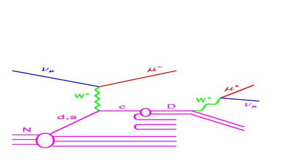
FIG. 1.: Dimuon production in $\nu$-nucleon DIS from scattering off a strange or down quark (LO QCD charm production).

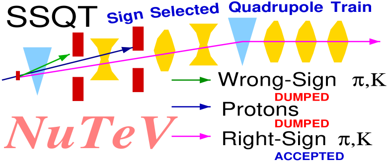
FIG. 2.: Schematic of the NuTeV beamline.

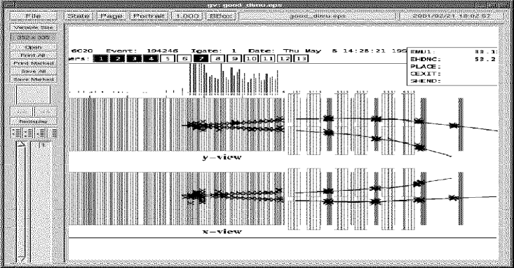
FIG. 3.: Typical dimuon event.

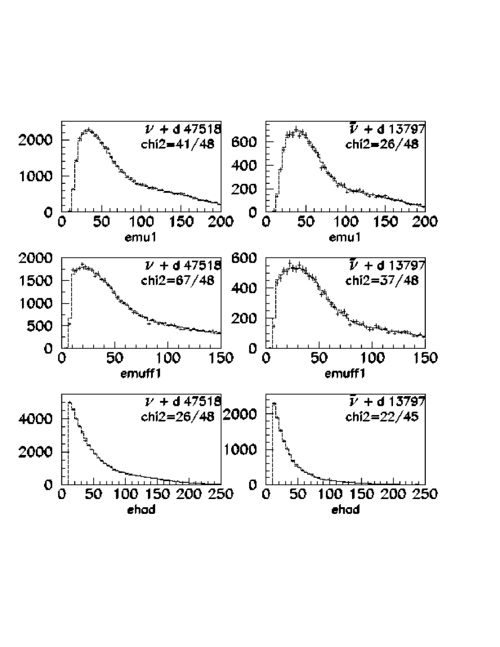
FIG. 4.: Charged-current Monte Carlo distributions (histograms) compared to data (points). Top: energy of the primary muon. Middle: energy of the primary muon entering the toroid. Bottom: hadronic energy. All energies are in GeV. Neutrino mode is shown on the left, anti-neutrinos on the right side of the plot. The $\chi^{2}$ per degree of freedom is shown for each distribution.

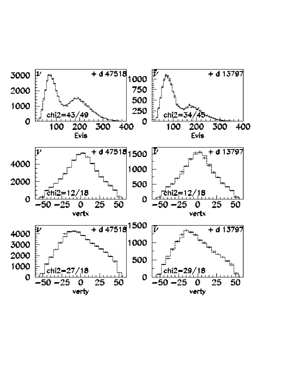
FIG. 5.: Charged-current Monte Carlo distributions (histograms) compared to data (points). Top: neutrino energy in GeV $E_{VIS}=E_{1\mu}+E_{2\mu}+E_{had}$. Middle: event vertex position in x plane. Bottom: event vertex position in y plane. Neutrinos are shown on the left, anti-neutrinos on the right. The $\chi^{2}$ per degree of freedom is shown for each distribution.

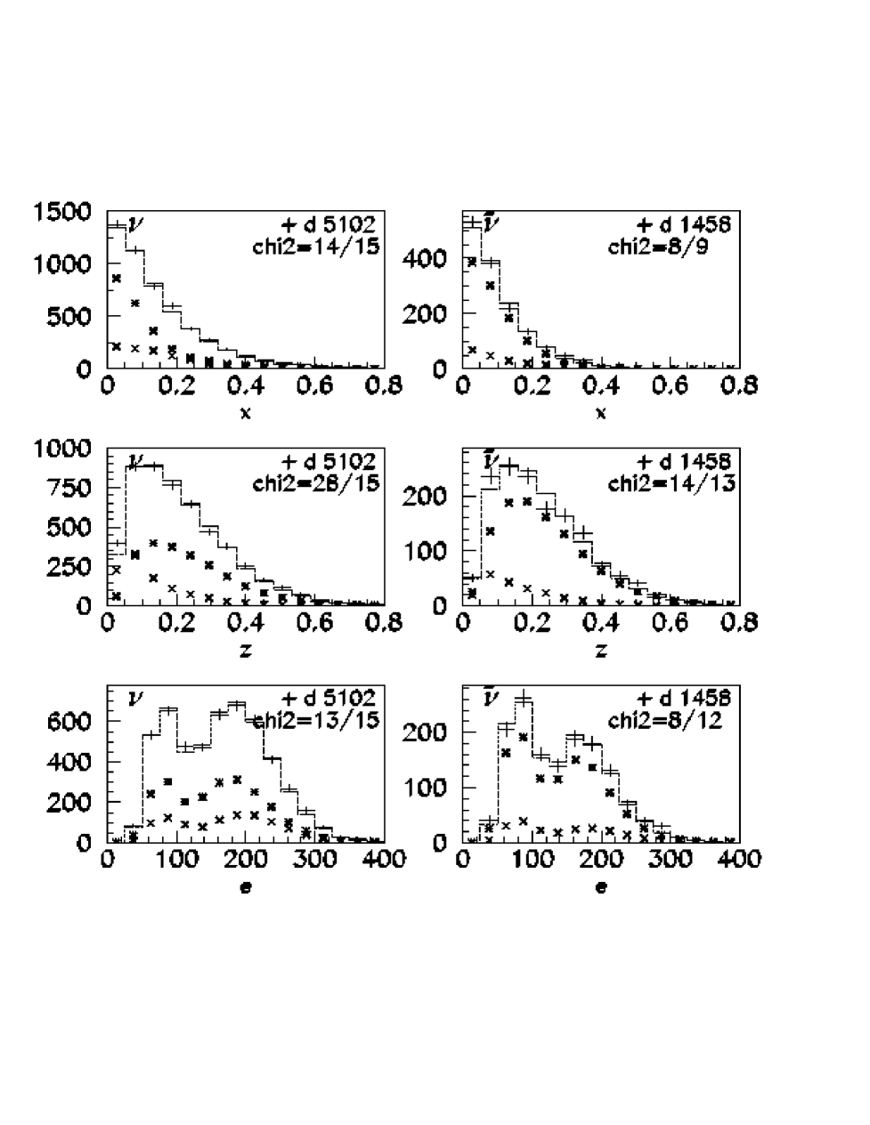
FIG. 6.: $x$, $z$, and $E$ distributions for dimuons (points) compared to Monte Carlo (histogram). Neutrinos are shown on the left, anti-neutrinos on the right. These distributions are used in the log-likelihood fit. The crosses show the Monte Carlo $\pi K$ background component, and the stars the strange sea contribution.

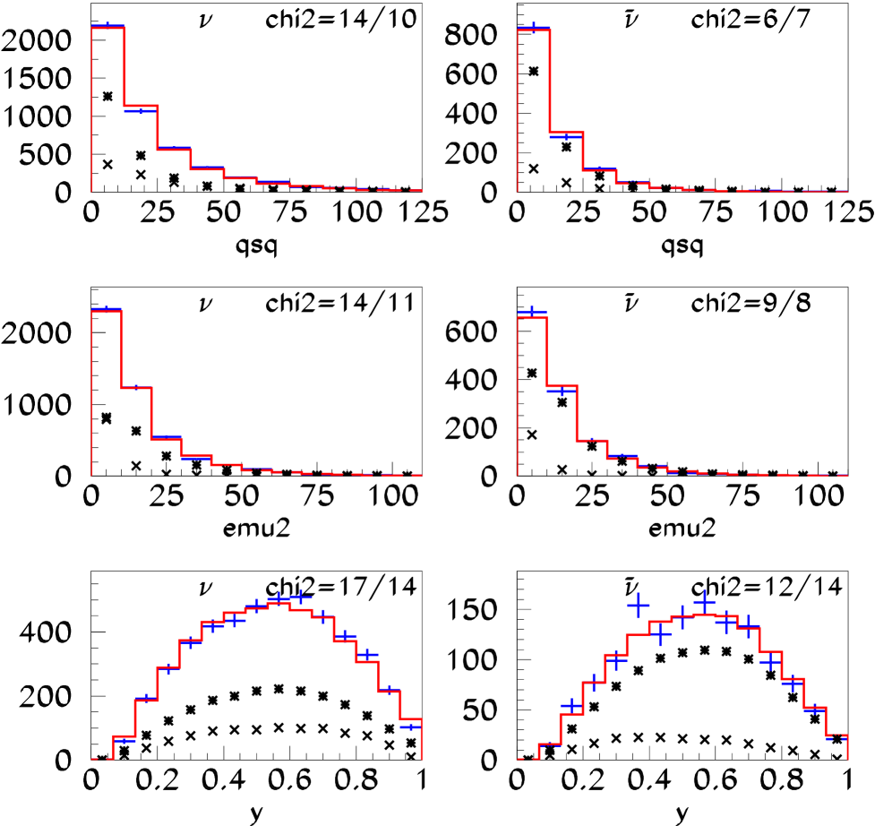
FIG. 7.: Dimuon data kinematic distributions (points) not used in the fit: $Q^{2}$ in GeV², $E_{\mu 2}$ in GeV, and $y$, from top to bottom. Neutrinos are shown on the left, anti-neutrinos on the right. The total Monte Carlo prediction is represented by the histogram, while the crosses show the $\pi K$ background component, and the stars the strange sea contribution.

FIG. 8.: $\sigma_{2\mu}(x)$ from NuTeV neutrinos, for various $E_{\nu}-y$ bins in units of charged-current $\sigma$. The cross-section extracted using the BGPAR model in the Monte Carlo is shown in squares, the circles correspond to extraction using the CTEQ model, and the triangles to the GRV model. The curves show the model prediction for GRV (dashed), CTEQ (dotted), and BGPAR (solid) after the models have been fit to the data.

FIG. 9.: $\sigma_{2\mu}(x)$ from NuTeV anti-neutrinos, for various $E_{\nu}-y$ bins in units of charged-current $\sigma$. The cross-section extracted using the BGPAR model in the Monte Carlo is shown in squares, the circles correspond to extraction using the CTEQ model, and the triangles to the GRV model. The curves show the model prediction for GRV (dashed), CTEQ (dotted), and BGPAR (solid) after the models have been fit to the data.

FIG. 10.: $\sigma_{2\mu}(x)$ from CCFR neutrinos, for various $E_{\nu}-y$ bins in units of charged-current $\sigma$. The cross-section extracted using the BGPAR model in the Monte Carlo is shown in squares, the circles correspond to extraction using the CTEQ model, and the triangles to the GRV model. The curves show the model prediction for GRV (dashed), CTEQ (dotted), and BGPAR (solid) after the models have been fit to the data.

FIG. 11.: $\sigma_{2\mu}(x)$ from CCFR anti-neutrinos, for various $E_{\nu}-y$ bins in units of charged-current $\sigma$. The cross-section extracted using the BGPAR model in the Monte Carlo is shown in squares, the circles correspond to extraction using the CTEQ model, and the triangles to the GRV model. The curves show the model prediction for GRV (dashed), CTEQ (dotted), and BGPAR (solid) after the models have been fit to the data.

FIG. 12.: Effective DOF and $\chi^{2}$ as a function of coverage area ${\cal C}$. The open symbols (dotted curve) show the $\chi^{2}$ obtained by fitting the cross-section table, while the stars (solid curve) show the effective DOF. The open squares on both curves show the result obtained by using the same grid on both smeared and unsmeared variables.

REFERENCES

• [1] J.ย M.ย Conrad, M.ย H.ย Shaevitz, and T.ย Bolton, Rev.ย Mod.ย Phys.ย 70, 1341 (1998).
• [2] M.ย A.ย G.ย Aivazis, F.ย I.ย Olness, and W.-K.ย Tung, Phys.ย Rev.ย D 50, 3085 (1994); M.ย A.ย G.ย Aivazis, J.ย C.ย Collins, F.ย I.ย Olness, and W.-K.ย Tung, ibid.ย 50, 3102 (1994).
• [3] M.ย Gluck, S.ย Kretzer, and E.ย Reya, Phys.ย Lett.ย B 380, 171 (1997); erratum ibid. 405, 391 (1997).
• [4] A.ย D.ย Martin et al., Eur.ย Phys.ย J.ย C2, 287 (1998).
• [5] A.ย Chuvakin, J.ย Smith, and W.ย L.ย vanย Neerven, Phys.ย Rev.ย D 61, 096004 (2000).
• [6] V.ย Barone et al., Phys.ย Lett.ย B328, 143 (1994).
• [7] R.ย Demina et al., Phys.ย Rev.ย D 62, 035011 (2000).
• [8] S.ย J.ย Brodsky and B.ย Ma, Phys.ย Lett.ย B 381, (317) (1996).
• [9] T.ย Sjostrand, Comput.ย Phys.ย Commun. 82, 74 (1994).
• [10] N.ย Ushida, et al., Phys.ย Lett.ย B206, 375 (1988); ibid, 206, 380 (1988).
• [11] T. Bolton, 1997, โ€œDetermining the CKM Parameters Vcd from $\nu$N Charm Production,โ€ KSU-HEP-97-04, e-print hep-ex/9708014 (August, 1997).
• [12] D.ย E.ย Groom et al., Eur.ย Phys.ย Jour.ย C 15, 110 (2000).
• [13] A.ย O.ย Bazarko et al., Z.ย Phys.ย C 65, 189 (1995).
• [14] S.ย A.ย Rabinowitz et al., Phys.ย Rev.ย Lett.ย 70, 134 (1993).
• [15] H.ย Abramowicz et al., Z.ย Phys.ย C 15, 19 (1982).
• [16] P.ย Vilain et al., Eur.ย Phys.ย J.ย C 11, 19 (1999).
• [17] P.ย Astier et al., Phys.ย Lett.ย B 486, 35 (2000).
• [18] P.ย Collins and T.ย Spiller, J.ย Phys.ย G 11, 1289 (1985).
• [19] C.ย Peterson et al., Phys.ย Rev.ย D27, 105 (1983).
• [20] A. Alton et al., โ€œSearch for Light-to-Heavy Quark Flavor Changing Neutral Currents in $\nu_{\mu}N$ and $\bar{\nu}_{\mu}N$ Scattering at the Tevatron,โ€ KSU-HEP-00-001, e-print hep-ex/0007059, to be published in Phys.ย Rev.ย D (July 31, 2000).
• [21] D.ย A.ย Harris et al., Nucl.ย Instrum.ย Meth.ย A 447, 377 (2000).
• [22] R.ย Brun et al., โ€œGEANT Detector Description and Simulation Library,โ€ CERN computing document CERN CN/ASD(1998).
• [23] D.ย Yu.ย Bardin and O.ย M.ย Fedorenko, Sov.ย J.ย Nucl.ย Phys. 30, 418 (1979).
• [24] G.ย Ingelman, A.ย Edin, and J.ย Rathsman, Comput.ย Phys.ย Commun. 101, 108 (1997).
• [25] P.ย Sandler, โ€œNeutrino Production of Same-Sign Dimuons at the Fermilab Tevatron,โ€ Ph.D. Thesis, Univ. of Wisconsin, 1992.
• [26] D.ย C.ย Carey, F.ย C.ย Iselin, โ€œDecay TURTLE (Trace Unlimited Rays Through Lumped Elements): A Computer Program for Simulating Charged Particle Beam Transport Systems, Including Decay Calculations,โ€ Fermilab preprint FERMILAB-PM-31 (1982).
• [27] H.ย W.ย Atherton et al., โ€œPrecise Measurements Of Particle Production by 400-GeV/c Protons in Beryllium Targets,โ€ CERN preprint CERN-80-07 (1980).
• [28] A.ย J.ย Malensek, โ€œEmpirical Formula For Thick Target Particle Production,โ€ Fermilab preprint FERMILAB-FN-0341 (1981).
• [29] M.ย Gluck, E.ย Reya, and A.ย Vogt, Z.ย Phys.ย C 67, 433 (1995).
• [30] H.ย L. Lai et al., Eur.ย Phys.ย J.ย C 12, 375 (2000).
• [31] H.ย Plothow-Besch, Comput.ย Phys.ย Commun.ย 75, 396 (1993).
• [32] A.ย J.ย Buras and K.ย J.ย F.ย Gaemers, Nucl.ย Phys.ย B 132, 259 (1978).
• [33] L.ย W.ย Whitlow et al., Phys.ย Lett.ย B 282, 475 (1992).
• [34] V.ย Barone, C.ย Pascaud, and F.ย Zomer, Eur.ย Phys.ย J.ย C 12, 243 (2000).