Electroweak and $B$ Physics Results from the Fermilab Tevatron Collider

Abstract

This writeup is an introduction to some of the experimental issues involved in performing electroweak and $b$ physics measurements at the Fermilab Tevatron. In the electroweak sector, we discuss $W$ and $Z$ boson cross section measurements as well as the measurement of the mass of the $W$ boson. For $b$ physics, we discuss measurements of $B^{0}/\overline{B^{0}}$ mixing and $CP$ violation. This paper is geared towards nonexperts who are interested in understanding some of the issues and motivations for these measurements and how the measurements are carried out.

1 Introduction

The Fermilab Tevatron collider is currently between data runs. The period from 1992-1996, known as Tevatron Run 1, saw both the CDF and DØ experiments accumulate approximately $110\,\rm pb^{-1}$ of integrated luminosity. These data sets have yielded a large number of results and publications on topics ranging from the discovery of the top quark to precise measurements of the mass of the $W$ boson; from measurements of jet production at the highest energies ever observed to searches for physics beyond the Standard Model.

This talk and subsequent paper focus on two aspects of the Tevatron program: electroweak physics and the physics of hadrons containing the bottom quark. Each of these topics is quite rich in its own right. It is not possible to do justice to either these topics in the space provided.

Also, there are a large number of sources for summaries of recent results. For example, many conference proceedings and summaries are easily accessible to determine the most up-to-date measurements of the mass of the $W$ boson. Instead of trying to summarize a boat-load of Tevatron measurements here, I will attempt to describe a few measurements in an introductory manner. The goal of this paper is to explain some of the methods and considerations for these measurements. This paper therefore is geared more towards students and non-experts. The goal here is not to comprehensively present the results, but to discuss how the results are obtained and what the important elements are in these measurements.

After a brief discussion of the Tevatron collider and the two collider experiments, we will discuss electroweak and $b$ physics at the Tevatron.

2 The Tevatron Collider

The Fermilab Tevatron collides protons($p$) and antiprotons ($\overline{p}$) at very high energy. In past runs, the $p\overline{p}$ center of mass energy was $\sqrt{s}=1.8\,\rm TeV$. It will be increased in the future to $2\,\rm TeV$. Until the Large Hadron Collider begins operation at CERN late in this decade, the Tevatron will be the highest energy accelerator in the world. The high energy, combined with a very high interaction rate, provides many opportunities for unique and interesting measurements.

Table 1: Some highlights in the history of the Fermilab Tevatron. This table lists primarily milestones associated with the collider program. In addition, there have been several Tevatron fixed-target runs, producing a wealth of physics results.

1969	ground breaking for National Accelerator Laboratory “Main Ring”
1972	200 GeV beam in the Main Ring
1983	first beam in the “Energy Doubler” $\Rightarrow$ “Tevatron”
1985	CDF observes first $p\overline{p}$ collisions
1988-89	Run 0, CDF collects $\sim$3$\,\rm pb^{-1}$
1992-93	Run 1A, CDF and DØ collect $\sim$20$\,\rm pb^{-1}$
1994-95	Run 1B, CDF and DØ collect $\sim$90$\,\rm pb^{-1}$
2001-02	Run 2 with new Main Injector and Recycler,
	upgraded CDF and DØ  expect 2000$\,\rm pb^{-1}$=2$\rm\,fb^{-1}$
2003-	Run 3, 15-30$\,\rm fb^{-1}$

The Tevatron has a history that goes back over $20$ years. Table 1 lists a few of the highlights. The original Fermilab accelerator, the “Main Ring”, was finally decommissioned in 1998 after more than 25 years of operation. In collider mode, the Main Ring served as an injector for the Tevatron. The Main Ring and Tevatron resided in the same tunnel of circumference of $\sim\!4\,$miles. The Tevatron now resides alone in this tunnel.

The Tevatron consists of approximately 1000 superconducting magnets. Dipole magnets are $\sim\!7\,\rm m$ in length, cooled by liquid helium to a temperature of $3.6\,\rm K$ and typically carry currents of over $4000\,\rm Amps$. Protons and anti-protons are injected into the Tevatron at an energy of $150\,\rm GeV$, then their energy is raised to the nominal energy which was $900\,\rm GeV$ per beam in the past and will be $980\,\rm GeV$ per beam for the upcoming run. During the period known as Run 1B, the Tevatron routinely achieved a luminosity that was more than 20 times the original design luminosity of $10^{30}\,\rm cm^{-2}s^{-1}$ [1].

The major upgrade in recent years has been the construction of the Main Injector which replaces the Main Ring. The Main Injector, along with another new accelerator component, the Recycler, will allow for much higher proton and antiproton intensities, and therefore higher luminosity than previously achievable. The anticipated Tevatron luminosity in the upcoming run will be a factor of $200$ beyond the original design luminosity for the Tevatron.

The CDF and DØ results presented here are from the $110\,\rm pb^{-1}$ of integrated luminosity collected in the period of $1992$-$1996$. The expectations for Run II are for a $20$-fold increase in the data sample by $2003$ ($2\,\rm fb^{-1}$). Beyond Run II, the goal is to increase the data sample by an additional factor of $10$ ($15$-$30\,\rm fb^{-1}$) by the time that the LHC begins producing results.

3 CDF and DØ

The CDF and DØ detectors are both axially symmetric detectors that cover about $98\%$ of the full $4\pi$ solid angle around the proton-antiproton interaction point. The experiments utilize similar strategies for measuring the interactions. Near the interaction region, tracking systems accurately measure the trajectory of charged particles. Outside the tracking region, calorimeters surround the interaction region to measure the energy of both the charged and neutral particles. Behind the calorimeters are muon detectors, that measure the deeply penetrating muons. Both experiments have fast trigger and readout electronics to acquire data at high rates. Additional details about the experiments can be found elsewhere [2, 3].

The strengths of the detectors are somewhat complementary to one another. The DØ detector features a uranium liquid-argon calorimeter that has very good energy resolution for electron, photon and hadronic jet energy measurements. The CDF detector features a $1.4\,\rm T$ solenoid surrounding a silicon microvertex detector and gas-wire drift chamber. These properties, combined with muon detectors and calorimeters, allow for excellent muon and electron identification, as well as precise tracking and vertex detection for $B$ physics.

4 Electroweak Results

Although many precise electroweak measurements have been performed at and above the $Z^{0}$ resonance at LEP and SLC, the Tevatron provides some unique and complementary measurements of electroweak phenomena. Some of these measurements include $W$ and $Z$ production cross sections; gauge boson couplings ($WW$,$W\gamma$,$WZ$,$Z\gamma$,$ZZ$); and properties of the $W$ boson (mass, width, asymmetries).

For the most part, both $W$ and $Z$ bosons are observed in hadron collisions through leptonic decays to electrons and muons, such as $W^{+}\rightarrow e^{+}\bar{\nu}_{e}$ and $Z^{0}\rightarrow\mu^{+}\mu^{-}$. The branching ratios for the leptonic decays of the $W$ and $Z$ are significantly smaller than the branching ratios for hadronic decays. There are about 3.2 hadronic $W$ decays for every $W$ decay to $e$ or $\mu$ and about 10 hadronic $Z$ decays for every $Z$ decay to $e^{+}e^{-}$ or $\mu^{+}\mu^{-}$. Unfortunately, the dijet background from processes like $qg\rightarrow qg$ and $gg\rightarrow q\overline{q}/gg$ (in addition to higher order processes) totally swamp the signal from $Z^{0}\rightarrow q\overline{q}$ and $W^{+}\rightarrow q\overline{q}^{\prime}$.

4.1 $W$ and $Z$ Production

The rate of production of $W$ and $Z$ bosons is an interesting test of the theories of both electroweak and strong interactions. The actual production rates are determined by factors that include the gauge boson couplings to fermions (EW) and the parton distribution functions and higher order corrections (QCD).

As an example analysis, we will discuss the measurement the $Z$ production cross-section from the $Z^{0}\rightarrow e^{+}e^{-}$ mode. The total number of events we observe will be:

$$N={\cal L}_{int}\cdot\sigma_{Z}\cdot Br(Z^{0}\rightarrow e^{+}e^{-})\cdot\epsilon_{ee}$$ (1)

where ${\cal L}$ is the instantaneous luminosity, ${\cal L}_{int}=\int{\cal L}dt$ is the integrated luminosity, $\sigma_{Z}=\sigma(p\overline{p}\rightarrow Z^{0}X)$ is the $Z$ boson production cross section, $Br(Z^{0}\rightarrow e^{+}e^{-})$ is the branching ratio for $Z^{0}\rightarrow e^{+}e^{-}$, and $\epsilon_{ee}$ is the efficiency for observing this decay mode. We have made the simplifying assumption that there are no background events in our signal sample. Let’s take each term in turn:

• ${\cal L}_{int}=\int{\cal L}dt$: the integrated luminosity is measured in units of $\rm cm^{-2}$ and is a measure of the total number of $p\overline{p}$ interactions. The instantaneous luminosity is measured in units of $\rm cm^{-2}s^{-1}$. In this case, “integrated” refers to the total time the detector was ready and able to measure $p\overline{p}$ interactions.

• $\sigma_{Z}=\sigma(p\overline{p}\rightarrow Z^{0}X)$: cross sections are measured in units of $\rm cm^{2}$ and are often quoted in units of “barns”, where $\rm 1b=10^{-24}\rm cm^{2}$. Typical electroweak cross sections measured at the Tevatron are in nanobarns ($\rm nb=10^{-9}\rm b$) or picobarns ($\rm pb=10^{-12}b$). The total cross section for $p\overline{p}$ at the Tevatron is about $70\,\rm mb=70\times 10^{-3}\rm b$. The cross section listed here is for any and all types of $Z$ boson production. The “$X$” includes the remaining fragments of the initial $p$ and $\overline{p}$, in addition to allowing for additional final state particles.

• $Br(Z^{0}\rightarrow e^{+}e^{-})$: The branching ratio is the fraction of $Z^{0}$ bosons that decay to a specific final state, $e^{+}e^{-}$ in this example.

• $\epsilon_{ee}$: Of the $Z^{0}$ bosons that are produced and decay to $e^{+}e^{-}$, not all of them are detected or accepted into the final event sample. Some of the events are beyond the region of space the detector covers in addition to the fact that the detector is not 100% efficient for detecting any signature.

Our ultimate goal is to extract $\sigma_{Z}$. Rearranging Equation 1, we have:

$$\sigma_{Z}={N\over{{\cal L}_{int}\cdot Br(Z^{0}\rightarrow e^{+}e^{-})\cdot\epsilon_{ee}}}.$$ (2)

From the data, we can count the number of signal events, $N$. To extract a cross section, we need to know the terms in the denominator as well:

• The luminosity is measured by looking at the total rate for $p\overline{p}\rightarrow p\overline{p}X$ in a specific and well-defined detector region. This rate is measured as a function of time and then integrated over the time the detector is live. The equation $N={\cal L}\sigma$ is used again, in this case we already know the total $p\overline{p}$ cross section($\sigma$), so we can use this equation to extract ${\cal L}$. At $e^{+}e^{-}$ machines, the measurement of the luminosity is quite precise, with a relative error of $1\%$ or less. For hadron machines, that level of precision is not possible. Typical relative uncertainties on the luminosity are $5$-$8\%$[4].

• The branching ratio for $Z^{0}\rightarrow e^{+}e^{-}$ is measured quite precisely by the LEP and SLC experiments. The world average value is used as an input here. The uncertainty on that value is incorporated into the ultimate uncertainty on the cross section.

• The efficiency for a final state like this is measured by a combination of simulation and control data samples. Primarily, data samples are used that are well understood. For example, $Z^{0}$ decays ($Z^{0}\rightarrow e^{+}e^{-}$ and $Z^{0}\rightarrow\mu^{+}\mu^{-}$) provide an excellent sample of electrons and muons for detector calibration. The high invariant mass of the lepton pair is a powerful handle to reject background.

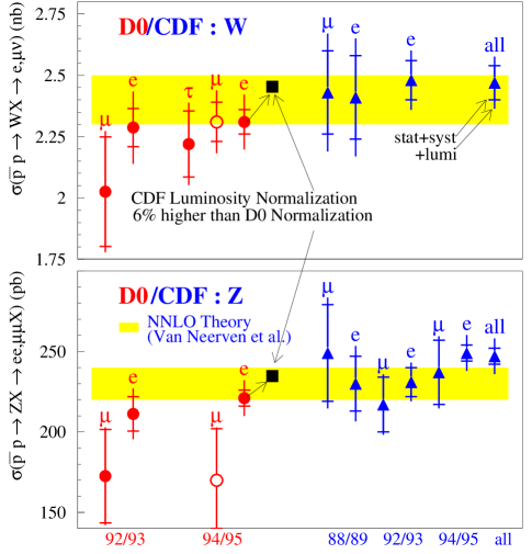
Fig. 1: Summary of DØ and CDF $W$ and $Z$ boson cross section measurements. The solid bands indicate the theoretical prediction. The circular points are the DØ results; the triangles are the CDF results. The two experiments use a different luminosity normalization.

Putting all of these factors together, it is possible to measure the total cross sections for $p\overline{p}\rightarrow WX$ and $p\overline{p}\rightarrow ZX$. These measurements are performed independently in both electron and muon modes. However, after the corrections for the efficiencies of each mode, the measurements should (and do) yield consistent measured values for the production cross section.

The results from DØ and CDF are represented in Fig. 1. The top plot is for $W$ production, the bottom plot for $Z$ production. The shaded region is the theoretical cross section. On both plots, the circular points are the DØ measurements, the triangles the CDF measurements. Part of the difference in the results from the two experiments arises from a different calculation of ${\cal L}_{int}$. If a common calculation were used, the DØ numbers would be $6\%$ larger than those presented. This shows that in fact the integrated luminosity is the largest systematic uncertainty on the cross sections. Details of these analyses may be found in the literature [5, 6].

4.2 ${\cal R}$ and the $W$ Width

One way to make the measurement more sensitive to the electroweak aspects of the $W$ and $Z$ production processes is to measure the cross section ratio. This ratio is often referred to as “${\cal R}$”, and defined as:

$${\cal R}\equiv\frac{\sigma(W)}{\sigma(Z)}\cdot\frac{Br(W\rightarrow\ell\nu)}{Br(Z\rightarrow\ell\ell)}$$

In taking the ratio of cross sections, the integrated luminosity (${\cal L}_{int}$) term and its uncertainty cancel. Other experimental and theoretical uncertainties cancel as well, making the measurement of ${\cal R}$ a more stringent test of the Standard Model. As we can see from Fig. 1, the ratio is about equal to $10$. This is confirmed by the results shown in Table 2.

Table 2: Summary of Tevatron measurements of ${\cal R}$, where ${\cal R}\equiv\frac{\sigma(W)}{\sigma(Z)}\cdot\frac{Br(W\rightarrow\ell\nu)}{Br(Z\rightarrow\ell\ell)}$.

	measured value of ${\cal R}$
DØ	$10.43\pm 0.15(\rm stat.)\pm 0.20(\rm syst.)\pm 0.10(\rm theory)$
CDF	$10.38\pm 0.14(\rm stat.)\pm 0.17(\rm syst.)$

The DØ result is for the electron final state [7]; the CDF result is for the electron and muon final states [8]. For the CDF result, the theoretical uncertainty is contained in the systematic uncertainty.

We can take this result one step further. The measured quantity is ${\cal R}$. Theoretically, the cross section ratio $\sigma(W)/\sigma(Z)$ is calculated with good precision. This can be understood by noting that the primary production of $Z$ bosons at the Tevatron arise from the reactions: $u\overline{u}\rightarrow Z^{0}$ and $d\overline{d}\rightarrow Z^{0}$, where the up and down quarks (and antiquarks) can be valence or sea quarks in the proton. An example of valence-valence production is shown in Fig. 2. For $W$ production, the primary contributions are $u\overline{d}\rightarrow W^{+}$ and $\overline{u}d\rightarrow W^{-}$. These reactions look quite similar to the $Z$ production mechanisms where a $u$ quark is replaced with a $d$ quark (or vice-versa). An example of valence-valence $W^{+}$ production is also shown in Fig. 2.

Although both $Z^{0}$ and $W^{\pm}$ are produced through quark-antiquark annihilation, the dominant contribution is not from the valence-valence diagrams shown in Fig. 2. The typical $q\overline{q}$ interaction energy for heavy boson production is the mass of the boson: $\sqrt{\hat{s}}\sim M_{Z,W}$. Since the heavy boson mass $M_{Z,W}\sim\!100\,\rm GeV=0.1\,\rm TeV$ and the $p\overline{p}$ center of mass energy is $\sqrt{s}\sim\!2\,\rm TeV$, the process requires the $q\overline{q}$ center of mass energy to be only $\sqrt{\hat{s}}/\sqrt{s}\simeq 5\%$ of the $p\overline{p}$ center of mass energy. In other words, if a quark and antiquark are each carrying $5\%$ of the proton (and antiproton) momentum, then there is sufficient collision energy to produce a heavy boson.

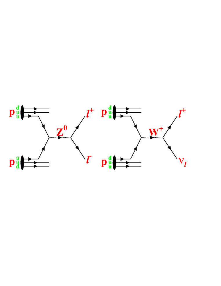
Fig. 2: Example $Z$ and $W$ production diagrams in high energy $p\overline{p}$ collisions. These figures show valence-valence production, which in fact is not dominant at Tevatron energies. The dominant production mechanism is quark-antiquark annihilation, where one quark(antiquark) is a valence quark and the other antiquark(quark) is a sea quark.

Both valence and sea quarks have a good probability for carrying a sufficient fraction of the proton’s energy to produce a gauge boson. In fact, the dominant production mechanism at the Tevatron is annihilation where the quark(antiquark) is a valence quark and the antiquark(quark) is a sea quark. The valence-sea production mechanism is about $4$ times larger than the valence-valence and sea-sea production mechanisms. It is coincidental that the valence-valence and sea-sea mechanisms are about equal at this energy. At higher energies, the sea-sea mechanism dominates; at lower energies, the valence-valence mechanism dominates [9].

The theoretical predictions for the production cross sections of $Z$ and $W$ bosons are not known to high precision. Strong interaction effects, such as the parton distribution functions and higher order diagrams lead to theoretical uncertainty. The ratio of cross sections is well calculated, however, because going from $Z$ production to $W^{+}$ production amounts to replacing an $\overline{u}$ with a $\overline{d}$. In addition, the gauge boson couplings to fermions are well measured. Combining these points makes the ratio of cross sections a much better determined quantity than the individual cross sections.

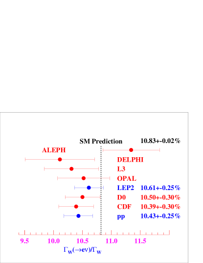
Fig. 3: Measurements of the branching ratio for $W\rightarrow e\nu_{e}$. The Tevatron results come from a measurement of ${\cal R}$ combined with the LEP measurement of $Br(Z^{0}\rightarrow e^{+}e^{-})$ and a theoretical calculation of $\sigma(W)/\sigma(Z)$.

Additionally, the branching ratio for $Z^{0}\rightarrow\ell^{+}\ell^{-}$ is well measured at LEP. Using our measured value of ${\cal R}$, inputting the theoretical value for $\sigma(W)/\sigma(Z)$ and using the LEP value for $Br(Z^{0}\rightarrow\ell^{+}\ell^{-})$, we can extract the branching ratio for $W\rightarrow\ell\nu$. This is shown in Fig. 3. The Tevatron results have similar uncertainties to the results from LEP2. As the uncertainties are reduced, this measurement will continue to be an important test of the Standard Model.

4.3 $W$ mass

The electroweak couplings and boson masses within the Standard Model may be completely specified by three parameters. Typically, those parameters are chosen to be $M_{Z}$ (the mass of the $Z^{0}$ boson), $G_{F}$, (the Fermi constant), and $\alpha_{QED}$ (the electromagnetic coupling constant). These three parameters are not required to be the inputs, though. For example, we could choose to use the charge of the electron ($e$), the weak mixing angle ($\sin^{2}\theta_{W}$) and the mass of the $W$ boson ($M_{W}$) as our inputs. At tree level (no radiative corrections, also known as Born level), any set of three parameters is sufficient to calculate the remaining quantities. The three chosen: $M_{Z}$, $G_{F}$ and $\alpha_{QED}$ are the ones measured experimentally with the highest precision.

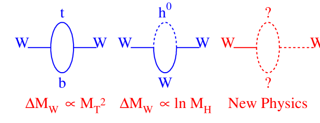
Fig. 4: Loop contributions to the $W$ mass. The $\Delta M_{W}$ denotes the shift in $W$ mass from the Born level value. The dependence upon the top quark mass is more dramatic than the dependence on the Higgs mass. New physics can appear in these loop corrections as well.

Therefore, at Born level, these three parameters are sufficient to exactly determine the mass of the $W$ boson. The true $W$ mass depends additionally on radiative corrections, the most important of which involve the top quark and the Higgs boson. Radiative corrections involving fermion or boson loops grow with the mass of the particle in the loop. This is why the top quark and Higgs boson masses are the most important corrections to the $W$ mass. These loop diagrams are shown graphically in Fig. 4.

The $W$ mass can be calculated with a high degree of precision and therefore simply measuring the $W$ mass provides a test of the Standard Model. Since there is additional uncertainty on the $W$ mass due to the unknown mass of the Higgs boson (or perhaps it doesn’t exist in the Standard Model form) the simple test of comparing the measured $W$ mass value to the prediction is not a high precision test. It is an important test, though, because deviations from the Standard Model predicted $W$ mass can arise through other non-Standard Model particles affecting the $W$ mass through loops.

In addition, when combined with the measured value for the top quark mass ($M_{t}$), we can constrain the Higgs mass. In saying that we can constrain the Higgs mass, this is implicitly assuming a Standard Model Higgs boson. This can be seen graphically in Fig 5, where electroweak results are plotted in the $M_{W}$,$M_{t}$ plane. The contour marked “Tevatron” shows the directly measured values for $M_{W}$ and $M_{t}$. The bands are contours of Standard Model calculations for $M_{W}$ versus $M_{t}$ for different masses of the Higgs boson. The current Tevatron region is consistent with the Standard Model and prefers a light Higgs boson.

Another way the $W$ mass tests the Standard Model is through self-consistency with other Standard Model measurements. For example, the LEP1, SLD, $\nu$N data contour in Fig. 5 arises from taking the electroweak measurements of $\sin^{2}\theta_{W}^{eff}$, $Z$ boson parameters and couplings and translating them into the $M_{W}$,$M_{t}$ plane. Right now, the three contours: $M_{W}$,$M_{t}$ from the Tevatron; $M_{W}$ from LEP2; and the LEP, SLD, $\nu$N contour are all consistent with one another and tend favor a light Higgs mass. It is conceivable that the contours could all be consistent with the Standard Model yet inconsistent with one another. An inconsistency of this type would indicate non-Standard Model physics.

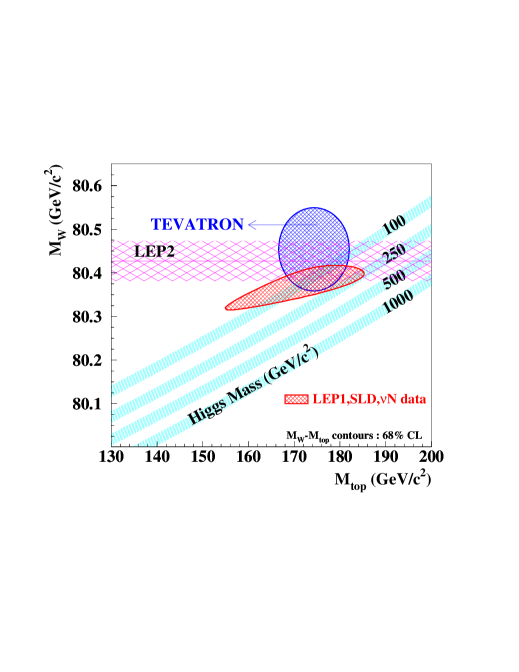
Fig. 5: A summary of precision electroweak measurements. The Tevatron contour is from direct measurements of $M_{W}$ and $M_{t}$. The horizontal band is the direct measurement of $M_{W}$ from LEP2. The oval contour arises from precision electroweak measurements of $\sin^{2}\theta_{W}^{eff}$, and $Z$ couplings and asymmetries translated into the $M_{W}$, $M_{t}$ plane. The bands are Standard Model contours for various values of the Higgs mass, $M_{H}$. It is clear that the experimental results are consistent with one another and currently favor a light Higgs boson.

The smaller the contours, the more stringent the constraints on the Higgs boson mass and the Standard Model tests. The goal of current and future experiments is to measure electroweak parameters as precisely as possible to further constrain and test the Standard Model. Currently, the crucial aspects of these measurements are the top quark mass and the mass of the $W$ boson.

4.3.1 The Measurement of $M_{W}$

As stated previously, the dominant mechanism for $W$ boson production is quark-antiquark annihilation ($q\overline{q}^{\prime}\rightarrow W^{\pm}$). The center of mass energy for this interaction, $\sqrt{\hat{s}}$ is much less than the $p\overline{p}$ center of mass energy of $\sqrt{s}=1.8\,\rm TeV$. This production mechanism leads to two important consequences:

1. The energies of the annihilating quark and antiquark are not equal, meaning the $W$ will be produced with a momentum component along the beam line ($p_{z}^{W}$). Another way to put this is to say that center-of-mass of the parton-parton collision is moving in the lab frame. The momentum of the partons transverse to the beam direction is effectively zero, so this center-of-mass motion is along the beam direction.

2. Since the remnants of the $p$ and $\overline{p}$ carry a large amount of energy in the far forward direction (along the beam line) it is not possible to accurately measure the $\hat{s}$ of the interaction. Therefore the initial $p_{z}$ of the $W$ is not known.

Fig. 6: A cartoon of a $W\rightarrow\ell\nu_{\ell}$ decay. The lepton is measured directly. The transverse momentum of the neutrino is inferred by the recoil energy ($u_{T}$).

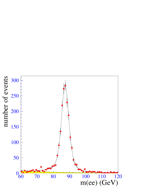
Fig. 7: The $Z^{0}$ mass as reconstructed in the mode $Z^{0}\rightarrow e^{+}e^{-}$ by the DØ detector. The shaded region at the bottom of the plot is the background contribution. The peak does not fall exactly on the true value of $M_{Z}$ because not all of the energy corrections have been applied to the data.

Because of these points, it is not possible to measure the mass of the $W$ boson based upon the collision energy, $\sqrt{\hat{s}}$. We must measure the $W$ mass by reconstructing the decay products.

Recall that we are dealing with $W\rightarrow e\nu_{e}$ and $W\rightarrow\mu\nu_{\mu}$ modes. The quantities associated with these decays that we can directly measure are:

• The momentum of the muon, $\vec{p}_{\ell}$.

• The recoil energy, $\vec{u}$.

The lepton momentum can be measured in three dimensions. The recoil energy can be measured in three dimensions, but since we do not know the initial $p_{Z}$ of the center of mass, the $z$ component of $\vec{u}$ and $\vec{p}_{\ell}$ are of no use to us. Since we know that (to very good approximation) $p_{x}^{W}+u_{x}=p_{y}^{W}+u_{y}=0$, we can implement conservation of momentum in the transverse $(x,y)$ plane and infer the transverse momentum of the neutrino. Since we do not know $p_{z}^{W}$, we can not infer the $p_{z}^{\nu}$ from momentum conservation. Even with three-dimensional measurements of $\vec{u}$ and $\vec{p}_{\ell}$, it is not possible to unambiguously determine the neutrino momentum in three dimensions. If it were possible to determine $\vec{p}_{\nu}$, then we could simply calculate the invariant mass of the $\ell$-$\nu_{\ell}$ and measure the $W$ mass from the resonance.

The case of $Z$ production as discussed above is quite similar to $W$ production. The difference, however, is that the $Z$ can decay to two charged leptons that we can measure in the detector. Figure 7 shows the reconstructed $Z$ mass in the mode $Z^{0}\rightarrow e^{+}e^{-}$ from the DØ detector. The $Z$ peak is clear and well-resolved, with small backgrounds.

In the case of the $W$ mass, the information we have is momentum of the lepton $\vec{p}^{\,\ell}$ and transverse momentum of the neutrino, $\vec{p}_{T}^{\,\nu}$, which was inferred from the transverse momentum of the lepton and the transverse recoil energy ($\vec{u}_{T}$).

From the transverse momenta of the lepton and the neutrino, we can calculate a quantity known as the “transverse mass”:

$$M_{T}^{W}=\sqrt{2p_{T}^{\ell}p_{T}^{\nu}(1-\cos\Delta\phi_{\ell,\nu})},$$

where $p_{T}^{\ell}$ and $p_{T}^{\nu}$ are the magnitudes of the lepton and neutrino transverse momenta and $\Delta\phi_{\ell,\nu}$ is the opening angle between the lepton and neutrino in the $x,y$ plane.

The transverse mass equation may look familiar. If we have two particles where we have measured the momenta in $3$ dimensions with momenta $\vec{p}_{1}$ and $\vec{p}_{2}$, then the invariant mass of those two particles in the approximation that the particles are massless is:

$$M_{1,2}=\sqrt{2p_{1}p_{2}(1-\cos\alpha)},$$

where $\alpha$ is the opening angle (in $3$-dimensions) between the two particles.

By comparing the two equations, we can see that the term “transverse mass” is accurate in that the calculation is identical to the invariant mass except only the transverse quantities are used. If the $W$ boson has $p_{Z}^{W}=0$, then the transverse mass is exactly the invariant mass. If the $W$ boson has $|p_{z}^{W}|>0$, then the transverse mass is less than the invariant mass. A $W$ boson transverse mass distribution is shown in Fig. 8.

Although not quite as clean as a full invariant mass, the transverse mass distribution quite clearly contains information about the $W$ mass. By fitting this distribution, it is possible to extract a precise measurement of the $W$ mass. There are three basic ingredients that determine the shape of the transverse mass distribution:

• $W$ boson production and decay.

• $p_{T}^{\ell}$ measurement.

• $u_{T}\Rightarrow p_{T}^{\nu}$ measurement.

Each of these items will be discussed in detail below. All of the details are ultimately combined into a fast Monte Carlo simulation that is able to generate transverse mass spectra corresponding to various values of the $W$ mass. The measured transverse mass distribution is then fit to the generated spectra and the $W$ mass is extracted from this fit.

In the following subsections, we discuss each of the elements required for precise $W$ mass determination.

4.3.2 $W$ boson production and decay

Modeling of the $W$ boson production and decay includes the Breit-Wigner lineshape, parton distribution functions, the momentum spectrum of the $W$ boson, the recoiling system and radiative corrections. The intrinsic width of the $W$ boson is about $2.1\,\rm GeV/c^{2}$ which must be included in the fit. The parton distribution functions (PDF) are representations of the distributions of valence quarks, sea quarks and gluons in the proton. The probability for specific processes as a function of $\hat{s}$ depend upon these distributions. Related to the PDFs and the production diagrams is the momentum distribution of the produced $W$ bosons. The model of the recoil system must be accurate. Higher order QED diagrams, such as $W\rightarrow\ell\nu\gamma$ are also included in the modeling.

4.3.3 $p_{T}^{\ell}$ measurement

This aspect is quite crucial in the $W$ mass determination. For muons, the transverse momentum is measured by the track curvature in the magnetic field. For electrons, it is more accurate to measure the energy (and infer the momentum) in the calorimeter because the resolution is better and bremsstrahlung tends to bias the tracking measurement of the curvature.

The energy scale is crucial. If we measure a muon with a transverse momentum of $30\,\rm GeV/c$, is the true momentum $30\,\rm GeV/c$? Is it $29.9\,\rm GeV/c$? Is it $30.1\,\rm GeV/c$? Also, the resolution is important to understand. For a measured momentum of $30\,\rm GeV/c$, we also need to know the uncertainty on that value, because it will smear out the transverse mass distribution. In reality, the resolution is a rather small effect, much smaller than the overall momentum scale.

To set the momentum/energy scale, we use “calibration” samples. The $J/\psi$, $\Upsilon$ and $Z^{0}$ masses are all known very precisely based upon measurements from other experiments. We can measure these masses using $\mu^{+}\mu^{-}$ and $e^{+}e^{-}$ final states to calibrate our momentum scale. If a muon measured with $p_{T}=29.9\,\rm GeV/c$ is truly a muon with $p_{T}=30.0\,\rm GeV/c$, then we will measure an incorrect $Z^{0}$ mass. This scale can be noted and ultimately corrected.

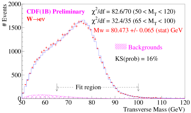
Fig. 8: The $W$ transverse mass in the mode $W\rightarrow e\nu_{e}$ as measured by CDF. The points are the data, the histogram is the fit. The hatched region shows the background contribution.

The $Z^{0}$ is particularly important for the $W$ mass measurement because both its mass and the production mechanism are very similar to that of the $W$. They are not identical, though, because the $Z^{0}$ is $10.7\,\rm GeV/c^{2}$ more massive than the $W$. Also, due to coupling and helicity considerations, the decay distributions are not identical between the two. They are quite close, however, and the $Z^{0}$ provides a crucial calibration point. The limiting factor then arises from the number of $Z^{0}$ decays available. As noted earlier, the ratio of observed leptonic $W$ decays to $Z$ decays (${\cal R}$) is about 10:1. In some cases, the limiting factor on the systematic uncertainty arises from the statistics of the $Z$ samples.

4.3.4 $u_{T}\Rightarrow p_{T}^{\nu}$ measurement

The recoil energy is required to infer the transverse momentum of the neutrino. Since the recoil energy is largely hadronic and contains both charged and neutral components, it must be measured with the calorimeter. All of the charged and neutral energy recoiling against the $W$ is included in the measurement, so all sources of calorimetric energy must be included in the model. The recoil distribution is affected by the collider environment, the resolution of the calorimeter, the coverage of the calorimeter and the ability to separate $u_{T}$ from $p_{T}^{\ell}$. At typical Tevatron luminosities, there are more than one, sometimes as many as six $p\overline{p}$ interactions per beam crossing. Most of these are inelastic events that have low transverse momentum. However, there is no way to directly separate out the contributions from other interactions from the contributions of the $W$ recoil. Instead, this must be modeled and the background level subtracted on an average basis. Uncertainty in this background subtraction leads to uncertainty in $M_{W}$.

The hadronic energy resolution of the calorimeter is much larger (i.e. worse) than the resolution on the lepton energy. Therefore, the resolution on the neutrino $p_{T}$ is determined by the hadronic energy resolution. The smaller this resolution, the less smeared the transverse mass distribution.

The coverage of the calorimeter must be understood, also, because some of the recoil can be carried away at very small angles to the beamline, where there is no instrumentation.

Finally, the recoil measurement is a sum of all calorimeter energy except the energy of the lepton. In the case of the muon channel, it is pretty straightforward to subtract the contribution from the muon. For the electron, some of the recoil energy is included in the electron energy cluster in the calorimeter simply because the recoil and electron energy “overlap”. This affects both the electron energy measurement and the $u_{T}$ measurement and therefore we must correct for that effect.

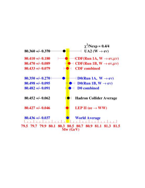
Fig. 9: Summary of direct measurements of the $W$ mass. The LEP II point is the combination of four experiments, while the CDF and DØ results are shown separately. The world average uncertainty is $37\,\rm MeV$.

4.3.5 $W$ Mass Summary

Each of these pieces needs to be fully and accurately modeled in order to understand how they effect the transverse mass distribution. There are many important aspects to this analysis, but the most important is the lepton energy scale. A great deal of work has gone into calibrating, checking and understanding the lepton energy scale.

Details of the DØ and CDF $W$ mass measurements may be found in Refs [10, 11]. For a recent compilation of the world’s $W$ mass measurements may be found in Ref [12].

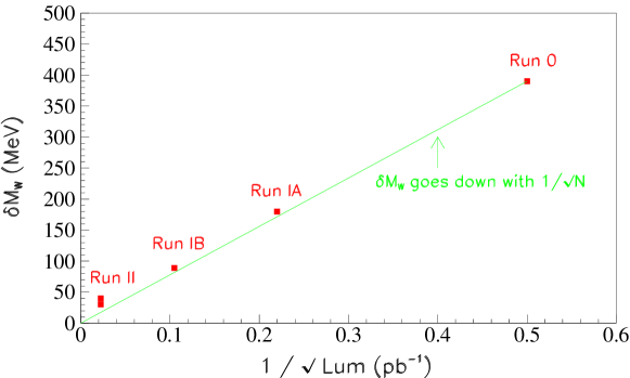
Fig. 10: The $W$ mass uncertainty as a function of data size. Both the statistical and systematic errors have continually fallen linearly as $1/\sqrt{N}$. This trend will continue in the future, although the ultimate Run II sensitivity will deviate from the line.

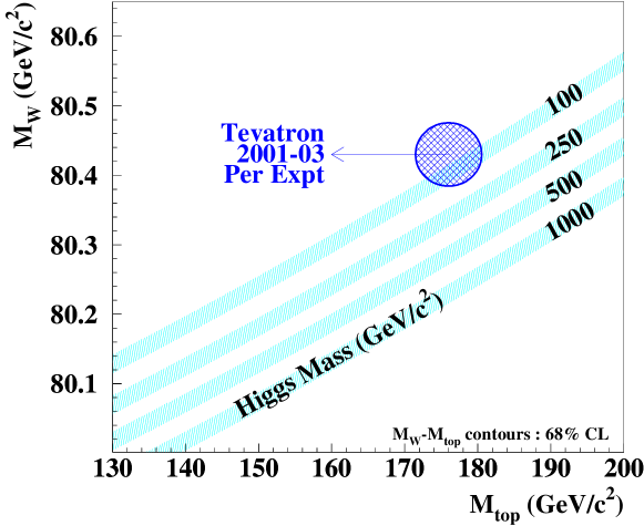
Fig. 11: The $M_{W}$ versus $M_{t}$ plot at the end of Run II. The central value is plotted as it currently stands. For Run II, we anticipate $\delta M_{W}\sim\!30\,\rm MeV$ and $\delta M_{t}\sim\!3\,\rm GeV$. These results will further test and constrain the Standard Model.

4.3.6 The Future

In addition to the Tevatron upgrades for Run II, the DØ and CDF collaborations are significantly upgrading their detectors [13, 14]. Figure 11 shows how the uncertainty on the $W$ mass has progressed over time. Since $N\propto{\cal L}_{int}$, the horizontal axis, plotted as $\sqrt{{\cal L}_{int}}$ is equivalent to $\sqrt{N_{W}}$, with $N_{W}$ being the number of identified $W$ boson decays. So far, the uncertainty on the $W$ mass has fallen linearly with $1/\sqrt{N_{W}}$. We expect the statistical uncertainty to fall as $1/\sqrt{N_{W}}$. The recent measurements of $M_{W}$ are not dominated by the statistical uncertainty, however. To maintain the $1/\sqrt{N_{W}}$ behavior of the total error, both the systematic and statistical uncertainties must fall as the statistics increase. This can be understood from the fact that many of the systematic uncertainties are limited by the statistics of the control samples, such as $Z^{0}\rightarrow\ell^{+}\ell^{-}$. As those samples grow, the systematic uncertainties fall.

Tevatron Run II is projected to move slightly away from the strict $1/\sqrt{N_{W}}$ behavior as some of the systematic uncertainties become limited by factors other than the statistics of the control samples. Nevertheless, the uncertainty is expected to be significantly reduced. The combined $W$ mass uncertainty from DØ and CDF is expected to be between $20$ and $40\,\rm Mev/c^{2}$ in Run II.

At the same time, the uncertainty on the top quark mass will also be reduced. Figure 11 also shows what the $M_{W},M_{t}$ plot could look like by about 2003. For this plot, we assume that the central measured value is the same as it is currently, simply to demonstrate how the uncertainty contours will look at that time. This compares quite favorably to the current version of this plot, shown previously in Fig. 5.

5 $B$ Physics Results

Since the first observation of a violation of charge-conjugation parity ($CP$) invariance in the neutral kaon system in 1964,[15] there has been an ongoing effort to further understand the nature of the phenomenon. To date, violation of $CP$ symmetry has not been directly observed anywhere other than the neutral kaon system. Within the framework of the Standard Model, $CP$ violation arises from a complex phase in the Cabibbo-Kobayashi-Maskawa (CKM) quark mixing matrix,[16] although the physics responsible for the origin of this phase is not understood. The goal of current and future measurements in the $K$ and $B$ meson systems is to continue to improve the constraints upon the mixing matrix and further test the Standard Model. Inconsistencies would point towards physics beyond the Standard Model.

In recent years, the importance and experimental advantages of the $B$ system have been emphasized.[17] The long lifetime of the $b$ quark, the large top quark mass and the observation of $B^{0}/\overline{B^{0}}$ mixing with a long oscillation time all conspire to make the $B$ system fruitful in the study of the CKM matrix. Three $e^{+}e^{-}$ $B$-factories running on the $\Upsilon$(4s) resonance in addition to experiments at HERA and the Tevatron indicate the current level of interest and knowledge to be gained by detailed study of the $B$ hadron decays.

This section is an introduction to $CP$ violation in the $B$ system, with a focus on experimental issues. After a some notational definitions, I will give a brief overview of the CKM matrix and $B^{0}/\overline{B^{0}}$ mixing. Following that, I will discuss experimental elements of flavor tagging, which is a crucial component in mixing and $CP$ asymmetry measurements. Our discussion of $CP$ violation in the $B$ system will be presented in the framework of the specific example of the measurement of $\sin 2\beta$ using $B^{0}/\overline{B^{0}}\rightarrow J/\psi K^{0}_{S}$ decays by the CDF Collaboration. Finally, I will briefly survey future measurements.

5.1 Notation

There are enough $B$’s and $b$’s associated with this topic that it is worthwhile to specifically spell out our notation. First of all, we will refer to bottom (antibottom) quarks using small letters: $b$ ($\overline{b}$). When we are referring to generic hadrons containing a bottom quark (e.g. $|b\overline{q}>$, where $q$ is any quark type), we will use a capital $B$ with no specific subscripts or superscripts.

In the cases where we are referring to specific bottom mesons or baryons, we will us the notation listed in Table 3. Neutral $B$ mesons follow the convention of the neutral kaon system, where $K^{0}=|\overline{s}d>$ and $\overline{K^{0}}=|s\overline{d}>$.

Table 3: $B$ mesons and baryons. This is an incomplete list, as there are excited states of the mesons and baryons (e.g. ${B^{*}}^{0}$). Also, a large number of $B$-baryon states are not listed (e.g. $\Sigma^{-}_{b}=|ddb>$).

name	$\overline{b}$ hadron	$b$ hadron
charged $B$ meson	$B^{+}=|\overline{b}u>$	$B^{-}=|b\overline{u}>$
neutral $B$ meson	$B^{0}=|\overline{b}d>$	$\overline{B^{0}}=|b\overline{d}>$
$B_{s}$ ($B$-sub-$s$) meson	$B^{0}_{s}=|\overline{b}s>$	$\overline{B^{0}_{s}}=|b\overline{s}>$
$B_{c}$ ($B$-sub-$c$) meson	$B^{+}_{c}=|\overline{b}c>$	$B^{-}_{c}=|b\overline{c}>$
$\Lambda_{b}$ (Lambda-$b$)	$\overline{\Lambda_{b}}=|\overline{u}\overline{d}\overline{b}>$	$\Lambda_{b}=|udb>$
$\Upsilon$ (Upsilon)	$\Upsilon=|\overline{b}b>$

5.2 Overview: the Cabibbo-Kobayashi-Maskawa Matrix

Within the framework of the Standard Model, $CP$ nonconservation arises through a non-trivial phase in the Cabibbo-Kobayashi-Maskawa (CKM) quark mixing matrix.[16] The CKM matrix $V$ is the unitary matrix that transforms the mass eigenstates into the weak eigenstates:

$$V= \pmatrix{V_{ud}&V_{us}&V_{ub}\cr V_{cd}&V_{cs}&V_{cb}\cr V_{td}&V_{ts}&V_{tb}\cr}$$ (3)

$$\simeq \pmatrix{1-{\lambda^{2}\over 2}&\lambda&A\lambda^{3}(\rho\!-\!i\eta)\cr-\lambda&1-{\lambda^{2}\over 2}&A\lambda^{2}\cr A\lambda^{3}(1\!-\!\rho\!-\!i\eta)&-A\lambda^{2}&1\cr}+{\cal O}(\lambda^{4}).$$ (4)

The second matrix is a useful phenomenological parameterization of the quark mixing matrix suggested by Wolfenstein,[18] in which $\lambda$ is the sine of the Cabibbo angle, $\lambda=\sin\theta_{C}\simeq 0.22$. The CKM matrix is an arbitrary three-dimensional rotation matrix. The only requirement a priori is that it be unitary – the value of the elements can take on any value so long as unitarity is preserved. The Wolfenstein parameterization arose based upon experimental results indicating that the matrix is nearly diagonal. Using experimental results on $V_{us}$ and $V_{cb}$ along with the unitarity requirement, Wolfenstein proposed the commonly-seen expansion shown here.

The condition of unitarity, $V^{\dagger}V=1$, yields several relations, the most important of which is a relation between the first and third columns of the matrix, given by:

$$V^{*}_{ub}V_{ud}+V^{*}_{cb}V_{cd}+V^{*}_{tb}V_{td}=0.$$ (5)

This relation, after division by $V^{*}_{cb}V_{cd}$, is displayed graphically in Fig. 12 as a triangle in the complex ($\rho$-$\eta$) plane, and is known as the unitarity triangle.[19] $CP$ violation in the Standard Model manifests itself as a nonzero value of $\eta$, the height of the triangle, which indicates the presence of an imaginary CKM component.

Fig. 12: The unitarity triangle. The horizontal axis is the real axis; the vertical axis is the imaginary axis. The apex of the triangle is $(\rho,\eta)$.

The “unitarity triangle” is simply a graph of a single point in the complex plane: $(\rho,\eta)$. We use the triangle to show how these two numbers are related to the CKM elements. Different experimental measurements are sensitive to different aspects of the unitarity triangle, i.e. they are sensitive to different combinations of $\rho$ and $\eta$.

Six unique triangles can be constructed from unitary relations (six more are complex conjugates of the first six.) The one shown here is the most useful because all of the sides are of ${\cal O}(\lambda)$, insuring that none of the three interior angles is near $0^{\circ}$ or $180^{\circ}$. The other triangles are “squashed” having one side ${\cal O}(\lambda^{2})$ or ${\cal O}(\lambda^{3})$ smaller than the other two sides.

The goal of current and future experiments in the $K$ and $B$ system is to measure as many aspects of the triangle as possible in as many ways as possible. Inconsistencies in these measurements will point to physics beyond the Standard Model and hopefully give us some indication from where these “fundamental constants” arise.

Based upon current measurements in the $K$ and $B$ system, such as $B^{0}/\overline{B^{0}}$ mixing, $K\rightarrow\pi^{\pm}\ell^{\mp}\nu$, $b\rightarrow u$ decays and $b\rightarrow c$ decays, the CKM solution indicates that the $CP$ violating phase is large. The fact that $CP$ violation in the $K$ system is small, ${\cal O}(0.1\%)$, arises from the fact that the magnitude of the matrix element $V_{td}$ is rather small. An alternate solution would be if the $CP$ violating phase were to be small and the magnitude of $V_{td}$ larger. Direct measurements of $CP$ violation in the $B$ system will permit clear distinction between the two cases.[20]

5.3 $B^{0}/\overline{B^{0}}$ Mixing

Mixing occurs in the neutral $K$ and $B$ systems because the electroweak eigenstates and the strong interaction eigenstates are not the same. If we start with a $B^{0}$ meson, then the probability that we will see a $B^{0}$($\overline{B^{0}}$) at a given time, $t$, is

$$P(B^{0}(t))=\frac{1}{2\tau}e^{-{t\over{\tau}}}(1+\cos(\Delta m_{d}t))$$

$$P(\overline{B^{0}}(t))=\frac{1}{2\tau}e^{-{t\over{\tau}}}(1-\cos(\Delta m_{d}t))$$ (6)

where $\tau$ is the $B^{0}$ lifetime and $\Delta m_{d}=m_{H}-m_{L}$, where $m_{H}$ and $m_{L}$ are the masses of the heavy and light weak eigenstates of the mesons. The mass difference $\Delta m_{d}$ in the $B^{0}/\overline{B^{0}}$ system is relatively small, therefore the mixing frequency is rather low. In units where $\hbar=c=1$, the mass difference is presented in units of $\rm ps^{-1}$. The current world average for $\Delta m_{d}$ is $0.487\pm 0.014\,\rm ps^{-1}$.[21] With this mass difference, the oscillation period for $B^{0}/\overline{B^{0}}$ is close to nine $B$ lifetimes.

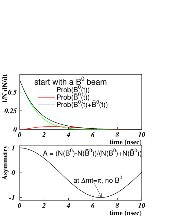
Fig. 13: $B^{0}/\overline{B^{0}}$ mixing. The top plot shows the probability functions for both $B^{0}$ and $\overline{B^{0}}$ as a function of time. At $t=0$, we have 100% $B^{0}$. As time increases, the mesons decay away exponentially $\propto e^{-{t\over{\tau}}}$, but some of the $B^{0}$ mesons become $\overline{B^{0}}$ mesons. The bottom plot shows the asymmetry so that the exponential effect has been removed. At $\Delta m_{d}t=\pi$ ($\Rightarrow t\simeq 4.4\tau\simeq 6.8\,\rm ps$, because the $B^{0}$ lifetime is $\tau=1.56\,\rm ps$.), all of the remaining mesons are $\overline{B^{0}}$!

Mixing is shown graphically in Fig. 13. When we begin with a beam of $B^{0}$ mesons, they disappear at a rate faster then $e^{-t/\tau}$, because some $B^{0}$ mesons are decaying and some are oscillating into $\overline{B^{0}}$ mesons. The sum of $B^{0}$ plus $\overline{B^{0}}$ decay at a rate $e^{-t/\tau}$.

Mixing in the neutral $B$ system is a second order $\Delta B=2$ transition that proceeds through “box” diagrams shown in Fig. 14. All up-type quarks ($u$,$c$ and $t$) are eligible to run around in the box, but the heavy top quark dominates because the amplitude is proportional to the mass of the fermion. As a consequence of this, there are two $top$-$W$-$down$ vertices ($V_{td}$) in the dominant box diagram. This will play a roll in $CP$ violation that we will discuss below.

The Feynman diagrams for $B^{0}_{s}/\overline{B^{0}_{s}}$ look quite similar with the exception that the $top$-$W$-$down$ vertices ($V_{td}$) are replaced by the $top$-$W$-$strange$ ($V_{ts}$) vertices. Since $|V_{ts}|>|V_{td}|$, the $B_{s}$ system oscillates much faster than does the $B_{d}$ system. Put another way, $\Delta m_{s}$ is much larger than $\Delta m_{d}$. The $B_{s}$ oscillates so quickly that the oscillation period is smaller than the experimental resolution on the decay time of the $B_{s}$. In other words, we can identify and distinguish between $B^{0}_{s}$ and $\overline{B^{0}_{s}}$ mesons at the time of decay, but the resolution of the decay time is not yet good enough to resolve the oscillations. The current experimental bound is $\Delta m_{s}>14\,\rm ps^{-1}$, which means that the $B_{s}$ fully mixes in less than 0.17 lifetimes!

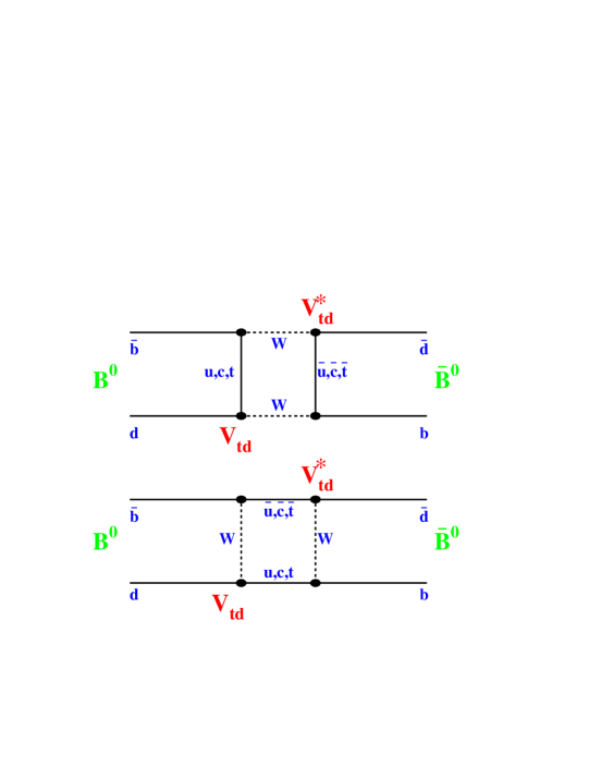
Fig. 14: $B^{0}/\overline{B^{0}}$ mixing diagrams. The diagrams shown are for $B^{0}$ oscillating into $\overline{B^{0}}$. The charge-conjugate process ($\overline{B^{0}}$ oscillating into $B^{0}$) takes place as well. The top quark dominates these $2^{nd}$ order weak transitions, which is why $V_{td}$ (and not $V_{ud}$ or $V_{cd}$) is shown at the vertices.

5.4 Flavor Tagging

To measure time-dependent mixing, it is necessary to know what the flavor of the meson was at the time of production and at the time of decay. For example, an “unmixed” event would be an event where a neutral $B$ meson was produced as a $B^{0}$ and decayed as a $B^{0}$. A “mixed” event would be one where a neutral $B$ meson was produced as a $B^{0}$ but decayed as a $\overline{B^{0}}$. Typically, mixing results are plotted (bottom plot of Fig. 13) as an asymmetry: ${\cal A}=(N_{unmixed}-N_{mixed})/(N_{unmixed}+N_{mixed})$. This has the advantage of removing the exponential term from the decay probabilities. Once plotted in this way, the functional form of the mixing is ${\cal A}=\cos\Delta m_{d}t$.

Experimentally, the determination of the flavor of the $B$ meson at the time of production and/or the time of decay is referred to as “flavor tagging”. Flavor tagging is an inexact science. The $B$ mesons have numerous decay modes, thanks in large part to the large phase space for production of light hadrons in the dominant $B\rightarrow D\rightarrow X_{s}$ decay, where $D$ and $X_{s}$ represent generic charmed and strange hadrons respectively. There is very low efficiency for fully reconstructing $B$ states. Therefore more inclusive techniques must be used to attempt to identify flavor.

Since flavor tagging is imprecise, it is crucial that we measure our success/failure rate. There are two parameters required to describe flavor tagging. The first is known as the tagging efficiency, $\epsilon$, which is simply the fraction of events that are tagged. For example, if we are only able to identify a lepton on $10\%$ of all of the events in our sample, then the lepton tagging efficiency is $10\%$. We can not distinguish a $B^{0}$ from a $\overline{B^{0}}$ in the other $90\%$ of the events because there was no lepton found to identify the flavor.

The second parameter is associated with how often the identified flavor is correct. A “mistag” is an event where the flavor was classified incorrectly. A mistag rate ($w$) of 40% is not unusual; while a mistag rate of 50% would mean that no flavor information is available – equivalent to flipping a coin. Another way to classify the success rate is through a variable called the “dilution” (${\cal D}$), defined as

$${\cal D}={N_{right}-N_{wrong}\over{N_{right}+N_{wrong}}}=1-2w$$ (7)

where $N_{right}$($N_{wrong}$) are the number of events tagged correctly (incorrectly). The term is dubbed “dilution” because it dilutes the true asymmetry:

$${\cal A}_{observed}={\cal D}{\cal A}_{true}$$ (8)

where ${\cal A}_{observed}$ is the experimentally measured asymmetry and ${\cal A}_{true}$ is the measurement of the real asymmetry we are trying to uncover.

In the following subsections we discuss some commonly used flavor tagging techniques. The methods outlined below are all utilized in mixing analyses. However, it is the initial state flavor tag that is important for $CP$ asymmetry measurements. The methods discussed here are summarized in Table 4.

Table 4: Methods of flavor tagging. These methods can be used in mixing analyses as well as $CP$ asymmetry measurements. In the case of $CP$ asymmetry measurements, the initial state flavor is the one of interest, as will be shown later.

method	initial/final state tag
exclusive reconstruction	final
partial reconstruction	final
lepton tagging	initial/final
jet charge tagging	initial
same side tagging	initial

5.4.1 Full/Partial Reconstruction

The flavor of the $B$ meson at the time of decay can be determined from the decay products. An example of this is $B^{0}\rightarrow D^{-}\pi^{+}$, with $D^{-}\rightarrow K^{+}\pi^{-}\pi^{-}$. This all-charged final state is an unambiguous signature of a $B^{0}$ meson at the time of decay. The drawback of the full reconstruction technique is that both the branching ratios to specific final states and reconstruction efficiencies are low.

To improve upon this, we can relax by performing a “partial” reconstruction. An example of this relating to the example above is to reconstruct $B^{0}\rightarrow D^{-}X$, with $D^{-}\rightarrow K^{+}\pi^{-}\pi^{-}$. In this case, the $X$ would include the state listed above, but would include all other decays of this type (e.g. $B^{0}\rightarrow D^{-}\pi^{+}\pi^{0}$.) Partial reconstruction is not as clean as full reconstruction. Since it is also possible to have $\overline{B^{0}}\rightarrow D^{-}X$, $B^{+}\rightarrow D^{-}X$, $B^{0}_{s}\rightarrow D^{-}X$ in addition to direct charm production, where $\overline{c}\rightarrow D^{-}$. Therefore the reconstruction of a $D^{-}$ meson is not an unambiguous signature for a $B^{0}$ meson. These other contributions must be accounted for in the extraction of $\Delta m_{d}$.

5.4.2 Initial State Tagging

Fig. 15: Initial state flavor tags. This example shows a reconstructed $J/\psi K^{0}_{S}$ final state. The other information in the event is used to identify the flavor of the $B^{0}$ or $\overline{B^{0}}$ at the time of production.

It is not possible to measure the flavor of a neutral $B$ meson at the time of production using full or partial reconstruction, because the decay only reflects the flavor of the final state. To perform initial state flavor tagging, two types of methods are employed. The first technique, known as opposite-side tagging, involves looking at the other $B$ hadron in the event. The second technique, known as same-side tagging, involves looking at the local correlation of charged tracks near the $B$.

Fig. 16: Same-side flavor tagging. In both cases shown above, a $\overline{b}$ quark is produced and ultimately ends up as a $B^{0}$ meson. In the left diagram, the $\overline{b}$ quark has grabbed a $d$ quark from the vacuum. The remaining $d$ quark has paired with a $\overline{u}$ quark to make a $\pi^{+}$. In the right diagram, the $\overline{b}$ quark grabs a $u$ quark to produce a radially-excited ${B^{**}}^{+}$ state. The ${B^{**}}^{+}$ then decays to a $B^{0}\pi^{+}$. In both cases, the $\pi^{+}$ is associated with a $B^{0}$ meson and a $\pi^{-}$ would be associated with a $\overline{B^{0}}$ meson. No information about the other $B$ hadron in the event is required.

In the case of opposite side tagging, we are taking advantage of the fact that $b$ and $\overline{b}$ are produced in pairs. If we determine the flavor of one $B$ hadron, we can infer the flavor of the other $B$ hadron. This is not perfect, of course, because in addition to the complications mentioned above, the opposite side $B$ hadron may have been a $B^{0}$ or $B^{0}_{s}$ and mixed.

Three types of opposite tagging are commonly used:

• lepton tagging: identify $B\rightarrow\ell\nu X$. The lepton carries the charge of the $b$.

• kaon tagging: identify $B\rightarrow D\rightarrow K$ ($b\rightarrow c\rightarrow s$). The strange particle carries the charge of the $b$.

• jet charge tagging: identify a “jet” associated with $B\rightarrow X$ and perform a momentum weighted charge sum. On average, the net charge of the jet will reflect the charge of the $b$.

Each of the methods has different experimental requirements and therefore different sets of positive and negative aspects. For example, with lepton tagging, the branching ratio and efficiency are rather low. In addition, there are mistags that come from $b\rightarrow c\rightarrow\ell$. On the other hand, lepton tags tend to have high dilution ($=$large ${\cal D}$). For jet charge tagging, the dilution is lower $=$small ${\cal D}$), but we are more likely to find a jet, which means a higher tagging efficiency.

By contrast, same-side tagging makes no requirement on the second $B$ hadron in the event. It instead takes advantage of the effects associated with hadronization. When a $\overline{b}$ quark becomes a $B^{0}$ meson, it must pair up with a $d$ quark. Since quark pairs pop-up from the vacuum, there is a $\overline{d}$ quark associated with the $d$ quark. Now if the $\overline{d}$ quark grabs a $u$ quark, then there is a $\pi^{+}$ associated with the $B^{0}$. This is shown in Fig. 16. An alternative path to the same correlation is through the production of a $B^{**}$ state. In either case, the correlation is: $B^{0}\pi^{+}$ and $\overline{B^{0}}\pi^{-}$. In our example above, if the $\overline{d}$ grabs a $d$ quark, then we have a $\pi^{0}$, in which case the first-order correlation is lost.

The same-side technique has the advantage of not relying on the second $B$ hadron in the event. The disadvantage is that, depending upon the hadronization process for a given event, the measured correlation may be absent or may be of the wrong sign. For example, the correlation would not be measurable if the mesons from the fragmentation chain were neutral. If the up quark in Fig. 16 were replaced by a down quark, then the associated meson would be a $\pi^{0}$. Likewise, wrong-sign correlations are present: if the up quark in Fig. 16 were replaced with a strange quark, then a ${K^{*}}^{0}$ would be produced, with ${K^{*}}^{0}\rightarrow K^{-}\pi^{+}$. If the $K^{-}$ is selected as the tagging track, then the wrong-sign is measured. This type of mistag can be reduced through the use of particle identification to separate charged kaons, pions and protons.

As will be seen below, initial state flavor tagging is a crucial aspect in measuring $CP$ asymmetries in the $B$ system. In the analysis we will discuss here, three of the four initial state tagging methods are used: lepton tagging, jet-charge tagging and same-side tagging.

5.5 $CP$ Violation Via Mixing

For Standard Model $CP$ violation to occur, we need an interference to expose the complex CKM phase. The $CP$ violating phase in $V_{td}$ can manifest itself through the $\Delta B=2$ box diagrams responsible for $B^{0}/\overline{B^{0}}$ mixing. In the Standard Model, the decay mode $B^{0}/\overline{B^{0}}\rightarrow J/\psi K^{0}_{S}$ is expected to exhibit mixing induced $CP$ violation. This final state can be accessed by both $B^{0}$ and $\overline{B^{0}}$. $CP$ violation in this case would manifest itself as:

$${dN\over{dt}}(B^{0}\rightarrow J/\psi K^{0}_{S})\neq{dN\over{dt}}(\overline{B^{0}}\rightarrow J/\psi K^{0}_{S})$$ (9)

where $J/\psi=|c\overline{c}>$, $K^{0}_{S}=\frac{1}{\sqrt{2}}(|d\overline{s}>+|s\overline{d}>)$ and the final state, $J/\psi K^{0}_{S}$ is a CP eigenstate:

$$CP|J/\psi K^{0}_{S}>=-|J/\psi K^{0}_{S}>$$ (10)

In the CKM framework, $CP$ violation occurs in this mode because the mixed decay and direct decay interfere with one another. This is shown in Fig. 17. An initial state $B^{0}$ can decay directly to $J/\psi K^{0}_{S}$, or it can mix into a $\overline{B^{0}}$ and then decay to $J/\psi K^{0}_{S}$. The interference between those two paths exposes the complex phase in the CKM matrix element $V_{td}$.

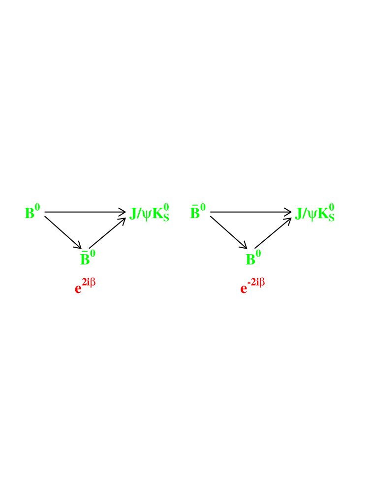
Fig. 17: $CP$ violation via mixing. Since both $B^{0}$ and $\overline{B^{0}}$ can decay to the $CP$ eigenstate $J/\psi K^{0}_{S}$, we have an interference between the mixed and unmixed decays. For example, if a meson is produced as a $B^{0}$ (shown on the left) and ultimately decays into $J/\psi K^{0}_{S}$, it could have decayed as a $B^{0}$ or mixed into a $\overline{B^{0}}$ before decaying. The process shown on the right is for an initial state $\overline{B^{0}}$. The interference exposes the phase in the CKM matrix element $V_{td}$, giving rise to $CP$ violation in the Standard Model.

When we produce $\overline{B^{0}}$ at $t=0$:

$${dN\over{dt}}(\overline{B^{0}}\rightarrow J/\psi K^{0}_{s})\propto e^{-t/\tau}(1+\sin 2\beta\sin\Delta m_{d}t)$$ (11)

If we produce $B^{0}$ at $t=0$:

$${dN\over{dt}}(B^{0}\rightarrow J/\psi K^{0}_{s})\propto e^{-t/\tau}(1-\sin 2\beta\sin\Delta m_{d}t)$$ (12)

Forming the asymmetry:

$$A_{CP}(t)={{dN\over{dt}}(\overline{B^{0}}\rightarrow J/\psi K^{0}_{S})-{dN\over{dt}}(B^{0}\rightarrow J/\psi K^{0}_{S})\over{{dN\over{dt}}(\overline{B^{0}}\rightarrow J/\psi K^{0}_{S})+{dN\over{dt}}(B^{0}\rightarrow J/\psi K^{0}_{S})}}$$

$$A_{CP}(t)=\sin 2\beta\ \sin(\Delta m_{d}t).$$ (13)

This is the time-dependent equation for the $CP$ asymmetry in this mode. The asymmetry as a function of proper time oscillates with a frequency of $\Delta m_{d}$. The amplitude of the oscillation is $\sin 2\beta$, where $\beta$ is the angle of the unitarity triangle shown earlier.

We can also perform the time-integral of equation 5.5:

$$A_{CP}\!\! =\!\! \!\!{\int{dN\over{dt}}(\overline{B}^{0}\rightarrow\psi K^{0}_{S})dt-\int{dN\over{dt}}(B^{0}\rightarrow\psi K^{0}_{S})dt\over{\int{dN\over{dt}}(\overline{B}^{0}\rightarrow\psi K^{0}_{S})dt+\int{dN\over{dt}}(B^{0}\rightarrow\psi K^{0}_{S})}dt}$$ (14)

$$A_{CP} = {N(\overline{B}^{0}\rightarrow\psi K^{0}_{S})-N(B^{0}\rightarrow\psi K^{0}_{S})\over{N(\overline{B}^{0}\rightarrow\psi K^{0}_{S})+N(B^{0}\rightarrow\psi K^{0}_{S})}}$$ (15)

Integrating equations 12 an 11 and substituting them, we get:

$$A_{CP} = {\Delta m_{d}\tau_{B}\over{1+(\Delta m_{d}\tau_{B})^{2}}}\cdot\sin 2\beta\$$ (17)

$$A_{CP} \simeq 0.47\sin 2\beta$$ (18)

This shows that we do not need to measure the proper time of the events. Integrating over all lifetimes still yields an asymmetry, although information is lost in going from the time dependent to the time-integrated asymmetry. The above formalism is true when the $B^{0}$ and $\overline{B^{0}}$ are produced in an incoherent state, as they are in high energy hadron collisions. At the $\Upsilon(4s)$, the $B^{0}$ and $\overline{B^{0}}$ are produced in a coherent state and the time-integrated asymmetry vanishes.[22]

5.6 Experimental Issues

The bottom line when it comes to $CP$ violation in the $B$ system is that you need to tell the difference between $B^{0}$ mesons and $\overline{B^{0}}$ mesons at the time of production. After identifying a sample of signal events, flavor tagging is the most important aspect of analyses of $CP$ violation.

In the case of the $J/\psi K^{0}_{S}$ final state, we have no way of knowing whether the meson was a $B^{0}$ or $\overline{B^{0}}$ as it decayed, nor do we need to know. The difference we are attempting to measure is the decay rate difference for mesons that were produced as $B^{0}$ or $\overline{B^{0}}$. In this case, we are tagging the flavor of the $B$ meson when it was produced.

The analysis we are going to discuss here is a measurement of the $CP$ asymmetry in $B^{0}/\overline{B^{0}}\rightarrow J/\psi K^{0}_{S}$ from the CDF experiment. Before discussing that measurement, we begin with by presenting some of the unique aspects to $b$ physics in the hadron collider environment.

5.6.1 $B$ Production and Reconstruction

First of all, the $b\overline{b}$ cross section is enormous, ${\cal O}(100\mu b)$, which means at typical operating luminosities, 1000 $b\overline{b}$ pairs are produced every second! The $b\overline{b}$ quarks are produced by the strong interaction, which preserves “bottomness”, therefore they are always produced in pairs. The transverse momentum ($p_{T}$) spectrum for the produced $B$ hadrons is falling very rapidly, which means that most of the $B$ hadrons have very low transverse momentum. For the sample of $B\rightarrow J/\psi K^{0}_{S}$ decays we are discussing here, the average $p_{T}$ of the $B$ meson is about $10\,\rm GeV/c$. The fact that the $B$ hadrons have low transverse momentum does not mean that they have low total momentum. Quite frequently, the $B$ mesons have very large longitudinal momentum (longitudinal being the component along the beam axis.) These $B$ hadrons are boosted along the beam axis and are consequently outside the acceptance of the detector.

Fig. 18: $B^{0}/\overline{B^{0}}\rightarrow J/\psi K^{0}_{S}$ event yield after the selection criteria discussed in the text have been applied. The data is plotted in units of “normalized mass”: $m_{norm}=(M_{fit}-M_{B})/\sigma_{fit}$, where $M_{fit}$ and $\sigma_{fit}$ are the four track fitted mass and uncertainty, respectively, and $M_{B}$ is the world average $B^{0}$ mass. Signal events show up with $M_{norm}$ near zero, while combinatoric background shows up uniformly across the plot.

For $b\overline{b}$ production, like $W$ production discussed previously, the center of mass of the parton-parton collision is not at rest in the lab frame. Even in the cases where one $B$ hadron is reconstructed (fully or partially) within the detector, the second $B$ hadron may be outside the detector acceptance.

To identify the $B$ mesons, we must first trigger the detector readout. Even though the $b\overline{b}$ production rate is large, it is about 1000 times below the generic inelastic scattering rate. In the trigger, we attempt to identify leptons: electrons and muons. In this analysis, we look for two muons, indicating that we may have had a $J/\psi\rightarrow\mu^{+}\mu^{-}$ decay.

Once we have the data on tape, we can attempt to fully reconstruct the $B^{0}/\overline{B^{0}}\rightarrow J/\psi K^{0}_{S}$ final state. The event topology that we are describing here can be seen in Fig. 15. To reconstruct $B\rightarrow J/\psi K^{0}_{S}$, we again look for $J/\psi\rightarrow\mu^{+}\mu^{-}$, this time with criteria more stringent than those imposed by the trigger. Once we find a dimuon pair with invariant mass consistent with the $J/\psi$ mass, we then look for the decay $K^{0}_{S}\rightarrow\pi^{+}\pi^{-}$. At this point, we require the dipion mass be consistent with a $K^{0}_{S}$ mass, and we also take advantage of the fact that the $K^{0}_{S}$ lives a macroscopic distance in the lab frame. Once we have both a $J/\psi$ and $K^{0}_{S}$ candidate, we put them all together to see if they were consistent with the decay $B^{0}/\overline{B^{0}}\rightarrow J/\psi K^{0}_{S}$. For example, the momentum of the $K^{0}_{S}$ must point back to the $B$ decay vertex, and the $B$ must point back to the primary (collision) vertex. After all of these selection criteria, we have a sample of 400 signal events with a signal to noise of about 0.7-to-1, as shown in Fig 18.

5.6.2 Flavor Tagging and Asymmetry Measurement

Now that we have a sample of signal events (intermixed with background), we must attempt to identify the flavor of the $B^{0}$ or $\overline{B^{0}}$ at the time of production using the flavor tagging techniques outlined above. For this analysis, we use three techniques: same-side tagging, lepton tagging and jet charge tagging. The lepton and jet charge flavor tags are looking at information from the other $B$ hadron in the event to infer the flavor of the $B$ we reconstructed. Table 5 summarizes the flavor tagging efficiency and dilution for each of the algorithms.

Table 5: Summary of tagging algorithms performance. All numbers listed are in percent. The efficiencies are obtained from the $B\to J/\psi K^{0}_{S}$ sample. The dilution information is derived from the $B^{\pm}\to J/\psi K^{\pm}$ sample.

tag side	tag type	efficiency ($\epsilon$)	dilution (${\cal D}$)	$\epsilon{\cal D}^{2}$
same-side	same-side	$73.6\pm 3.8$	$16.9\pm 2.2$	$2.1\pm 0.5$
opposite side	soft lepton	$5.6\pm 1.8$	$62.5\pm 14.6$	$2.2\pm 1.0$
	jet charge	$40.2\pm 3.9$	$23.5\pm 6.9$	$2.2\pm 1.3$

With the sample of events, the proper decay time and the measured flavor for each event, we are ready to proceed. In practice, we are measuring ${\cal A}(t)$:

$${\cal A}(t)={1\over{{\cal D}}}\left({N_{-}-N_{+}\over{N_{-}+N_{+}}}\right)={1\over{{\cal D}}}A_{raw}(t)$$ (19)

where $N_{-}$($N_{+}$) are the number of negative (positive) tags. A negative tag indicates a $\overline{B^{0}}$, while a positive tag indicates a $B^{0}$. We do not write $\overline{B^{0}}$ and $B^{0}$ in the equation, though, because not every negative tag is truly a $\overline{B^{0}}$.

We arrive at the quantity ${\cal A}_{raw}$ using the $J/\psi K^{0}_{S}$ data, but to get to the measured asymmetry, we must also know ${\cal D}$. We can measure ${\cal D}$ using control samples and Monte Carlo, but it can not be extracted from the $J/\psi K^{0}_{S}$ data. Since typical dilutions are about $20\%$, that means that the raw asymmetry is 1/5 the size of the measured asymmetry. The higher the dilution (the more effective the flavor tagging method) the closer the raw asymmetry is to the measured asymmetry. We can classify the statistical uncertainty on the asymmetry as:

$$(\delta{\cal A})^{2}=(\delta{\cal A}_{raw}/{\cal D})^{2}+({\cal A}_{raw}/{\cal D})^{2}(\delta{\cal D}/{\cal D})^{2}$$ (20)

where $\delta{\cal D}$ is the uncertainty on the dilution and $\delta{\cal A}_{raw}$ is the statistical uncertainty on the raw asymmetry. Ignoring (for the moment) the presence of background in our sample, $(\delta{\cal A}_{raw})_{stat}=1/\sqrt{N_{tagged}}=1/\sqrt{\epsilon N_{sig}}$, where $\epsilon$ is the flavor tagging efficiency discussed previously and $N_{sig}$ is the number of signal events. More realistically, we can not neglect the presence of background, and the statistical uncertainty on the measured asymmetry is: $(\delta{\cal A}_{raw})_{stat}={1\over{\sqrt{\epsilon N_{sig}}}}\sqrt{{N_{sig}+B\over{N_{sig}}}}$. The first term in Equation 20 is the “statistical” uncertainty on the asymmetry and is of the form: $\delta{\cal A}=1/\sqrt{\epsilon{\cal D}^{2}N_{sig}}$. Not only does the dilution factor degrade the raw asymmetry, it also inflates the statistical error. Think of it this way: we have events that we are putting into two bins–a $B^{0}$ bin and a $\overline{B^{0}}$ bin. When we tag an event incorrectly (mistag), we take it out of one bin and put it into the other bin. Not only do we have one less event in the correct bin, we have one more event in the incorrect bin! This hurts our measurement more than had we simply removed the event from the correct bin and thrown it away.

In reality, there are several complications to this measurement:

• Our data sample has both signal and background events in it. For an event in the signal region, we don’t know a priori if it is signal or background.

• We are using multiple flavor tagging algorithms. Each algorithm has a different ${\cal D}$ associated with it. Some events are tagged by more than one algorithm, and those two tags may agree or disagree.

• Due to experimental acceptance, not every event in our sample has a precisely determined proper decay time.

• Due to experimental acceptance, the efficiencies for positive and negative tracks are not identical (although the correction factor is tiny.)

We handle these effects with a maximum likelihood fit that accounts for the probability that any given event is signal versus background and tagged correctly versus incorrectly. In doing so, we not only account for the multiple flavor tagging algorithms and the background in our data, but the correlations between all of these elements is handled as well.[23]

Fig. 19: The true asymmetry (${\cal A}_{C}P(t)=\sin 2\beta\sin\Delta m_{d}t$) as a function of lifetime for $B\rightarrow J/\psi K^{0}_{S}$ events. The data points are sideband-subtracted and have been combined according to the effective dilution for single and double-tags. The events are shown in the rightmost point are those that do not have precision lifetime information.

5.6.3 Results

The final result of our analysis is show in Fig. 19. The points are the $J/\psi K^{0}_{S}$ data, after having subtracted out the contribution from the background. The data has also been corrected for the flavor tagging dilutions. The solid curve is the fit to the data of the functional form: ${\cal A}_{CP}=\sin 2\beta\sin\Delta m_{d}t$, with $\Delta m_{d}$ constrained to the world average value. The amplitude of the oscillation is $\sin 2\beta$. The single point to the right shows all events that do not have a precisely measured lifetime. As shown earlier, the time-integrated asymmetry is nonzero, therefore these events are quite useful in extracting $\sin 2\beta$.

The result of this analysis is:

$$\sin 2\beta=0.79{+0.41\atop-0.44}\,\rm(stat.+syst.)$$

This is consistent with the expectation of $\sin 2\beta=0.75$ based upon indirect fits to other data. This result rules out $\sin 2\beta=0$ at the 93% confidence level, not sufficient to claim observation of $CP$ violation in the $B$ system. On the other hand, this is the best direct evidence to date for $CP$ violation in the $B$ system. When broken down into statistical and systematic components, the uncertainty is $\delta(\sin 2\beta)=\pm 0.39(\rm stat.)\pm 0.16(\rm syst.)$. The total uncertainty is dominated by the statistics of the sample and efficacy of the flavor tagging. The systematic uncertainty arises from the uncertainty in the dilution measurements ($\delta{\cal D}$.) However, the uncertainty on the dilution measurements are actually limited by the size of the data samples used to measure the dilutions. In other words, the systematic uncertainty on $\sin 2\beta$ is really a statistical uncertainty on the ${\cal D}$’s. As more data is accumulated in the future, both the statistical and systematic uncertainty in $\sin 2\beta$ will decrease as $1/\sqrt{N}$.

Figure 20 shows the contours which result from global fits to measured data in the $B$ and $K$ system.[24, 25] The dashed lines originating at (1,0) are the two solutions for $\beta$ corresponding to $\sin 2\beta=0.79$. The solid lines are the $1\sigma$ contours for this result. Clearly the result shown here is in good agreement with expectations.

The uncertainty on the $\sin 2\beta$ result presented here is comparable to the uncertainties from recent measurements by the Belle and Babar collaborations[22, 26]. While none of the measurements are yet to have the precision to stringently test the Standard Model, the fact that this measurement can be made in two very different ways is interesting. The hadron collider environment has an enormous $b\overline{b}$ cross section, but backgrounds make flavor tagging difficult. In the $e^{+}e^{-}$ environment, the production cross section is much smaller, but the environment lends itself more favorably to flavor tagging. These facts make the measurements performed in the different environments complementary to one another.

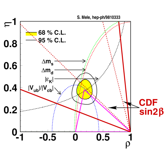
Fig. 20: The experimental determination of $\rho$ and $\eta$. The curves are based upon experimental measurements of $V_{ub}$, $\epsilon_{K}$, $B^{0}_{d}$ and $B^{0}_{s}$ mixing. The contours are the result of the global fit to the data.[25] The dashed lines originating at (1,0) are the two solutions for $\beta$ corresponding to $\sin 2\beta=0.79$. The solid lines are the $1\sigma$ contours for this result.

5.7 The Future

The Fermilab Tevatron is scheduled to Run again in 2001. Both CDF[14] and DØ[13] detectors are undergoing massive upgrades in order to handle more than a factor of 20 increase in data. In addition, $e^{+}e^{-}$ $B$-factories at Cornell (CLEO-III),[27] KEK (Belle)[28] and SLAC (BaBar)[29] are all currently taking data. Finally, Hera-B,[30] a dedicated $B$ experiment at DESY, also will begin taking data in 2001.

On the timescale of 2003-2004, there could be as many as 5 different measurements of $\sin 2\beta$, all of them with an uncertainty of $\delta(\sin 2\beta)\raisebox{-4.30554pt}{\mbox{$\mbox{}\stackrel{{\scriptstyle\textstyle<}}{{\sim}}\mbox{}$}}0.1$. Putting these together would yield a world average measurement with an uncertainty of $\delta(\sin 2\beta)\raisebox{-4.30554pt}{\mbox{$\mbox{}\stackrel{{\scriptstyle\textstyle<}}{{\sim}}\mbox{}$}}0.05$. Although this alone will provide an impressive constraint upon the unitarity triangle, it will not be sufficient to thoroughly test the Standard Model for self-consistency. On the same timescale, improvements are required in the lengths of the sides of the triangle, as well as other measurements of the angles. Finally, there are measurements of other quantities that are not easily related to the unitarity triangle that are important tests of the Standard Model.

The following is a list of some of the measurements that will be undertaken and/or improved-upon in the coming years (this is an incomplete list):

• $CP$ asymmetries in other modes: e.g.

  • $B^{0}/\overline{B^{0}}\rightarrow\pi^{+}\pi^{-}$;

  • $B^{0}_{s}/\overline{B^{0}_{s}}\rightarrow J/\psi\phi$;

  • $B^{0}_{s}/\overline{B^{0}_{s}}\rightarrow K^{+}K^{-}$;

  • $B^{0}_{s}/\overline{B^{0}_{s}}\rightarrow D_{s}^{\pm}K^{\mp}$;

  • $B^{0}/\overline{B^{0}}\rightarrow D^{+}D^{-}$.

• $B^{0}_{s}/\overline{B^{0}_{s}}$ mixing.

• rare $B$ decays: e.g. $B^{\pm}\rightarrow\mu^{+}\mu^{-}K^{\pm}$; $B^{0}\rightarrow\mu^{+}\mu^{-}$.

• radiative $B$ decays: e.g. $B^{0}\rightarrow K^{*}\gamma$; $B^{0}_{s}\rightarrow\phi\gamma$.

• improved measurements of $V_{ub}$: e.g. $B\rightarrow\pi\pi$; $B\rightarrow\rho\ell\nu$.

• mass and lifetime of the $B_{c}$ meson.

• mass and lifetimes of the $B$ baryons: e.g. $\Lambda_{b}=|udb>$.

It will take many years and a body of measurements to gain further insights into the mechanisms behind the CKM matrix and $CP$ violation.

Advances in kaon physics over the last 40 years and advances in $B$ physics in the last 25 years have put us on track to carry out these measurements in the very near future. These measurements will hopefully bring us to a more fundamental understanding to the mechanism behind $CP$ violation.

References

- [1] http://www-bd.fnal.gov/runII/index.html
- [2] The CDF Collaboration (F. Abe et al.), Nucl. Instr. & Meth A271, 387 (1988); http://www-cdf.fnal.gov/.
- [3] The DØ Collaboration (S. Abachi et al.), Nucl. Instr. & Meth A338, 185 (1994); http://www-d0.fnal.gov/.
- [4] D. Cronin-Hennessy, A. Beretvas and P. Derwent, Nucl. Instr. & Meth A443, 37 (2000);
- [5] The CDF Collaboration (T. Affolder et al.), Phys. Rev. Lett. 84, 845 (2000); The CDF Collaboration (F. Abe et al.), Phys. Rev. D59, 052002 (1999).
- [6] The DØ Collaboration (B. Abbott et al.), Phys. Rev. D60, 052003, (1999).
- [7] The DØ Collaboration (B. Abbott et al.), Phys. Rev. D61, 072001, (2000).
- [8] The CDF Collaboration (F. Abe et al.), Phys. Rev. D52, 2624 (1995).
- [9] E. Berger, F. Halzen, C.S. Kim and S. Willenbrock, Phys. Rev. D40, 83 (1989).
- [10] The DØ Collaboration (B. Abbott et al.), Phys. Rev. D58, 092003, (1998); The DØ Collaboration (B. Abbott et al.), Phys. Rev. D62, 092006, (2000).
- [11] The CDF Collaboration (T. Affolder et al.), FERMILAB-PUB-00-158-E, (2000), submitted to Phys.Rev.D.
- [12] The LEP Electroweak Working Group, http://lepewwg.web.cern.ch/LEPEWWG/.
- [13] The DØ Collaboration, FERMILAB-Pub-96/357-E (1996).
- [14] The CDF-II Collaboration, FERMILAB-Pub-96/390-E (1996); The CDF-II Collaboration Fermilab-Proposal-909 (1998).
- [15] J.H. Christenson et al., Phys. Rev. Lett. 13, 138 (1964).
- [16] N. Cabibbo, Phys. Rev. Lett. 10, 531 (1963); M. Kobayashi and T. Maskawa, Prog. Theor. Phys. 49, 652 (1973).
- [17] A.B. Carter and A.I. Sanda, Phys. Rev. Lett. 45, 952 (1980); Phys. Rev. D 23, 1567 (1981); I.I. Bigi and A.I. Sanda, Nucl. Phys. B193, 85 (1981); Nucl. Phys. B281, 41 (1987).
- [18] L. Wolfenstein, Phys. Rev. Lett. 51, 1945 (1983).
- [19] L.-L. Chau and W.-Y. Keung, Phys. Rev. Lett. 53, 1802 (1984); C. Jarlskog and R. Stora, Phys. Lett. B 208, 268 (1988); J.D. Bjorken, Phys. Rev. D 39, 1396 (1989).
- [20] Y. Nir, IASSNS-HEP-99-96 (1999), hep-ph/9911321.
- [21] Particle Data Group (C. Caso et al.), Eur. Phys. J. C 3, 1 (1998); LEP Oscillations Working Group, http://lepbosc.web.cern.ch/LEPBOSC/.
- [22] C. Hearty, these proceedings.
- [23] CDF Collaboration (T. Affolder et al.), Phys. Rev. D 61:072005 (2000).
- [24] S. Herrlich and U. Nierste, Phys. Rev. D 52, 6505 (1995); A. Ali and D. London, Nucl. Phys. B (Proc. Suppl.) 54A, 297 (1997); P. Paganini et al., Phys. Scr. 58, 556 (1998).
- [25] S. Mele, Phys. Rev. D 59, 113011 (1999).
- [26] N. Katayama, these proceedings.
- [27] CLEO-III Collaboration, CLNS 94/1277 (1994).
- [28] BELLE Collaboration, KEK Report 95-1 (1995).
- [29] BaBar Collaboration, SLAC-Report-95-457 (1995).
- [30] HERA-B Collaboration, DESY-PRC 95/01 (1995).