A Measurement of the Decay Asymmetry Parameters in $\Xi_{c}^{0}\rightarrow\Xi^{-}\pi^{+}$

Abstract

Using the CLEO II detector at the Cornell Electron Storage Ring we have measured the $\Xi_{c}^{0}$ decay asymmetry parameter in the decay $\Xi_{c}^{0}\rightarrow\Xi^{-}\pi^{+}$. We find $\alpha_{\Xi_{c}^{0}}\alpha_{\Xi}=0.26\pm 0.18\mbox{(stat)}^{+0.05}_{-0.04}\mbox{(syst)}$, using the world average value of $\alpha_{\Xi}=-0.456\pm 0.014$ we obtain $\alpha_{\Xi_{c}^{0}}=-0.56\pm 0.39\mbox{(stat)}^{+0.10}_{-0.09}\mbox{(syst)}$. The physically allowed range of a decay asymmetry parameter is $-1<\alpha<+1$. Our result prefers a negative value: $\alpha_{\Xi_{c}^{0}}$ is $<0.1$ at the 90% CL. The central value occupies the middle of the theoretically expected range but is not yet precise enough to choose between models.

The weak interactions underlying hadronic charm quark weak decay are straightforward to describe theoretically, but complications arise because the quarks are bound inside hadrons by the strong force. These interactions, which are described by the theory of quantum chromodynamics (QCD), are very difficult to predict using perturbative methods because the strong coupling is large at the typical energies of charm decays. Compared to charm mesons, charm baryons offer new information for two reasons: first, non-factorizable contributions to the decay amplitude are important; W-exchange diagrams can contribute without the helicity suppression that decreases their contribution to pseudoscalar meson decays, and internal W emission is expected to be significant. The relative importance of these effects is believed to be responsible for both the observed lifetime hierarchy of the charm baryons and the relatively shorter lifetime of charm baryons compared to charm mesons. Second, parity violation in charm baryon decays is readily observable because the decay of the daughter hyperon also violates parity. In consequence a variety of models  [1] are used to predict both the decay rate and degree of parity violation in charm baryon decays. To constrain the models it is important to provide as much experimental information as possible.

Parity violation occurs in hyperon and charm baryon ${1\over 2}^{+}\rightarrow{1\over 2}^{+}0$ decays due to the existence of two orbital angular momentum decay amplitudes of opposite parity. The experimental observable is an asymmetry in the angular decay distribution due to interference between the two amplitudes. In the decays $\Lambda_{c}^{+}\rightarrow\Lambda\pi^{+}$ and $\Xi^{-}\rightarrow\Lambda\pi^{-}$ both followed by $\Lambda\rightarrow p\pi^{-}$, the $\Lambda$ is produced with a polarization equal to

$${\bf P_{\Lambda}}={(\alpha_{B}+\hat{\bf\Lambda}\cdot{\bf P_{B}})\hat{\bf\Lambda}-\beta_{B}(\hat{\bf\Lambda}\times{\bf P_{B}})-\gamma_{B}\hat{\bf\Lambda}\times(\hat{\bf\Lambda}\times{\bf P_{B}})\over(1+\alpha_{B}\hat{\bf\Lambda}\cdot{\bf P_{B}})}$$ (1)

where $\bf P_{B}$ is the parent baryon polarization, $\alpha_{B},~{}\beta_{B}$ and $~{}\gamma_{B}$ are the parent baryon asymmetry parameters and ${\bf\hat{\Lambda}}$ is a unit vector along the $\Lambda$ momentum in the parent baryon frame  [2]. If the parent baryon polarization is unobserved, or if the parent baryon is not polarized, Equation  1 reduces to ${\bf P_{\Lambda}}=\alpha_{B}{\bf\hat{\Lambda}}$. The angular distribution of a proton from the decay of a $\Lambda$ is therefore

$${dN\over d\cos\theta_{\Lambda}}\propto 1+\alpha_{B}\alpha_{\Lambda}\cos\theta_{\Lambda}$$ (2)

where $\theta_{\Lambda}$ is the angle between the proton momentum vector in the $\Lambda$ rest frame and ${\bf\hat{\Lambda}}$, and $\alpha_{\Lambda}$ is the $\Lambda$ decay asymmetry, which measures the degree of parity violation in $\Lambda$ decay. Experimentally, a fit to equation  2 determines a product of decay asymmetries. For example, in $\Xi^{-}\rightarrow\Lambda\pi^{-}$, $\alpha_{B}=\alpha_{\Xi^{-}}$; since $\alpha_{\Lambda}$ is well measured ($\alpha_{\Lambda}=0.642\pm 0.013$  [3] ), $\alpha_{\Xi^{-}}$ can be extracted.

Equation  2 has also been used to extract the decay asymmetry of the $\Lambda_{c}$ in several decay modes. For example in $\Lambda_{c}^{+}\rightarrow\Lambda\pi^{+}$, $\alpha_{B}=\alpha_{\Lambda_{c}^{+}}$. In the massless fermion limit the chirality of the weak interaction corresponds to $\alpha=-1$, however, the interplay between the strong and weak interactions in the weak decay alters the value of $\alpha$. The decay asymmetry in $\Lambda_{c}^{+}\rightarrow\Lambda\pi^{+}$ is relatively well measured, the world average value is $\alpha_{\Lambda_{c}^{+}}=-0.98\pm 0.19$ [3], which is consistent with the naive V-A expectation. This result had been predicted by Heavy Quark Effective Theory (HQET) in conjunction with the factorization hypothesis [4]. Most pole and quark models [1], also predict large negative values of $\alpha_{\Lambda_{c}^{+}}$.

In this letter we measure the $\Xi_{c}^{0}$ decay asymmetry parameter in the decay $\Xi_{c}^{0}\rightarrow\Xi^{-}\pi^{+}$ for the first time. For $\Xi_{c}^{0}\rightarrow\Xi^{-}\pi^{+}$ theoretical predictions cover a larger range: $-1<\alpha_{\Xi_{c}^{0}}<-0.38$  [1]. The decay of $\Xi_{c}^{0}$ is a three step process where parity violation occurs at each decay stage: $\Xi_{c}^{0}\rightarrow\Xi^{-}\pi^{+}$, $\Xi^{-}\rightarrow\Lambda\pi^{-}$, $\Lambda\rightarrow p\pi^{-}$. The differential rate is therefore given by [5]:

$${dN\over d\cos\theta_{\Xi}d\cos\theta_{\Lambda}}\propto 1 + \alpha_{\Xi_{c}^{0}}\alpha_{\Xi}\cos\theta_{\Xi}+\alpha_{\Lambda}\alpha_{\Xi}\cos\theta_{\Lambda}$$ (3)

$$+ \alpha_{\Lambda}\alpha_{\Xi_{c}^{0}}\cos\theta_{\Xi}\cos\theta_{\Lambda}$$ (4)

where in addition to the terms previously defined: $\theta_{\Xi}$ is the angle between the $\Lambda$ momentum vector in the $\Xi^{-}$ rest frame and the $\Xi^{-}$ momentum vector in the $\Xi_{c}^{0}$ rest frame as shown in Fig. 1. Equation  4 reduces to the familiar form of Equation  2 when integrated over $\cos\theta_{\Lambda}$.

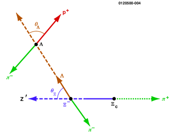
FIG. 1.: Definition of the angles $\theta_{\Xi}$ and $\theta_{\Lambda}$ in $\Xi_{c}^{0}\rightarrow\Xi^{-}\pi^{+}$. The decay of each particle is drawn in its own rest frame.

The data sample in this study was collected with the CLEO II detector  [6] at the Cornell Electron Storage Ring (CESR). The integrated luminosity consists of 4.83 $fb^{-1}$ taken at and just below the $\Upsilon(4S)$ resonance, corresponding to approximately 5 million $e^{+}e^{-}\rightarrow c\overline{c}$ events.

We search for the decay $\Xi_{c}^{0}\rightarrow\Xi^{-}\pi^{+}$ in $e^{+}e^{-}\rightarrow c\bar{c}$ events by reconstructing the decay chain $\Xi_{c}^{0}\rightarrow\Xi^{-}\pi^{+}$, $\Xi^{-}\rightarrow\Lambda\pi^{-}$, $\Lambda\rightarrow p\pi^{-}$.

The $\Lambda$ is reconstructed by requiring two oppositely charged tracks to originate from a common vertex. The positive track is required to be consistent with a proton hypothesis. The momentum of the $\Lambda$ candidate is calculated by extrapolating the charged track momenta to the secondary vertex. The invariant mass of $\Lambda$ candidates is required to be within three standard deviations (3$\sigma$ = 6.0 MeV/c²) of the known $\Lambda$ mass. Track combinations which satisfy interpretation as $K_{s}^{0}\rightarrow\pi^{+}\pi^{-}$ are rejected. Combinatoric and $B$ decay backgrounds are reduced by requiring the momentum of $\Lambda$ candidates be greater than 800 MeV/c.

The $\Xi^{-}$ is reconstructed in the $\Lambda\pi^{-}$ decay mode. $\Xi^{-}$ candidates are formed by combining each $\Lambda$ candidate with a negatively charged track consistent with a pion hypothesis. The $\Xi^{-}$ candidate vertex is formed from the intersection of the $\Lambda$ momentum vector and the negatively charged track. To obtain the $\Xi^{-}$ momentum, and $\Lambda\pi$ invariant mass, the momentum of the charged track is recalculated at the new vertex. The invariant $\Lambda\pi^{-}$ mass is fit to a double Gaussian signal shape with parameters fixed from a GEANT  [7] based Monte Carlo (MC) simulation of the detector, and a first order Chebyshev polynomial to describe the combinatorial background. We find $8434\pm 109$ events consistent with $\Xi^{-}\rightarrow\Lambda\pi^{-}$ with an invariant mass of $1322.0\pm 0.03$ MeV/c² and width $\sigma_{av}=2.5$ MeV/c², where $\sigma_{av}$ is the weighted average width of the double Gaussian. The mean and width are in agreement with the MC simulation.

To reconstruct $\Xi_{c}^{0}$ candidates all $\Xi^{-}$ candidates are combined with positively charged tracks consistent with a pion hypothesis. Since charm fragmentation is a relatively hard process, the $\Xi_{c}^{0}$ spectrum from $e^{+}e^{-}\rightarrow c\bar{c}$ is also fairly stiff. We therefore use a scaled momentum cut, $x_{p}>0.5$ to reduce combinatoric background. This cut also eliminates charmed baryons from decays of B mesons. Fig.  2 shows the invariant mass distribution of $\Xi^{-}\pi^{+}$ combinations. The $\Xi^{-}\pi^{+}$ invariant mass distribution is fit to a double Gaussian to describe the signal and a first order Chebyshev polynomial to describe the combinatorial background, where the parameters of the double Gaussian are fixed by MC simulation. The shaded histogram is wrong sign (WS) random $\Xi^{-}\pi^{-}$ combinations. There are less WS than right sign (RS) random combinations due to charge conservation.

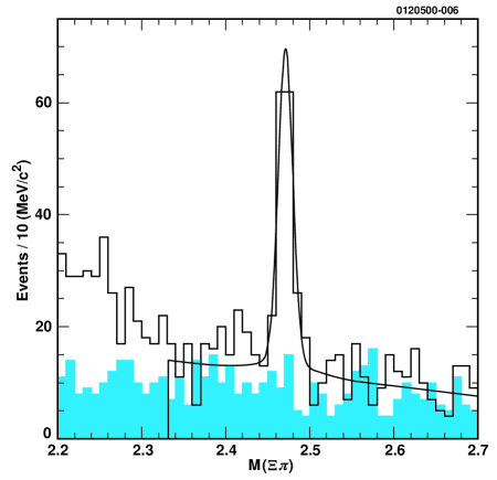
FIG. 2.: Invariant $\Xi^{-}\pi^{+}$ mass distribution. The shaded histogram is wrong sign (WS) random $\Xi^{-}\pi^{-}$ combinations.

The excess of right sign events over wrong sign events below M($\Xi^{-}\pi^{+}$) $=2.33$ GeV/c² is due to feedthrough from $\Xi_{c}^{+,0}\rightarrow\Xi^{-}n(\pi),\ n>1,$ where one or more pions are missing. The kinematic limit for feedthrough is $M(\Xi_{c}^{0})-M(\pi)=2.3304$ GeV/c². To simplify the fit to M($\Xi^{-}\pi^{+}$) the feedthrough region is excluded. We find $138\pm 14$ $\Xi_{c}^{0}\rightarrow\Xi^{-}\pi^{+}$ candidates with a mass of $2470.6\pm 1.0$ MeV/c² and width $\sigma_{av}=10$ MeV/c². The mean and width are in agreement with MC simulation. We require that the invariant mass of $\Xi_{c}^{0}$ candidates be within 30 MeV/c² (3 $\sigma_{av}$) of the known $\Xi_{c}^{0}$ mass.

MC simulation shows that the difference between generated and reconstructed values of $\cos\theta_{\Xi}$ and $\cos\theta_{\Lambda}$ has both Gaussian and symmetric non-Gaussian components. The resolution in $\cos\theta_{\Xi,\Lambda}$, $\sigma(\cos\theta_{\Xi},\Lambda)$, defined to be the average of the rms variance of the Gaussian and of the non-Gaussian component, weighted by the relative normalizations of the two components is: $\sigma(\cos\theta_{\Xi})=0.014$ and $\sigma(\cos\theta_{\Lambda})=0.030$.

The decay asymmetry parameter in $\Xi_{c}^{0}\rightarrow\Xi^{-}\pi^{+}$ is measured in a two dimensional unbinned maximum loglikelihood fit to the two-fold decay angular distribution of Equation  4, in a manner similar to  [8]. This technique enables a multi-dimensional likelihood fit to be performed to variables modified by experimental acceptance and resolution. The probability function of the signal, $\Gamma_{s},$ is determined by generating one high statistics MC sample of $\Xi_{c}^{0}\rightarrow\Xi^{-}\pi^{+}$, $\Xi^{-}\rightarrow\Lambda\pi^{-}$, $\Lambda\rightarrow p\pi^{-}$ with a known value of $\alpha_{\Xi_{c}^{0}}$ and the world average values of $\alpha_{\Xi}$ and $\alpha_{\Lambda}$. The generated events are processed through the detector simulation, off-line analysis programs, and selection criteria. Using the generated angles, accepted MC events are weighted by the ratio of the decay distribution for a trial value of $\alpha_{\Xi_{c}^{0}}$ to that of the generated distribution. By such weighting, a likelihood may be evaluated for each data event for trial values of $\alpha_{\Xi_{c}^{0}}$, and a fit performed. The probability for each event is determined by sampling $\Gamma_{s}$ using a search area centered on each data point. The size of the area is chosen such that the systematic effect from a finite search area is small and the required number of MC events is not prohibitively high.

Background is incorporated into the fitting technique by constructing the log-likelihood function:

$$\ln{\mathcal{L}}=\sum_{i=1}^{N}ln(P_{S}\Gamma_{S}+P_{B}\Gamma_{B})$$ (5)

where $N$ is the number of events in the signal region and $P_{S}$ and $P_{B}$ are the probabilities that events in this region are signal and background respectively. The probability distribution of background in the signal region, $\Gamma_{B}$, is determined from ($\Xi^{-}\pi^{+}$) mass sidebands above and below the signal region. The sidebands are: 2.5004 $<$ M($\Xi^{-}\pi^{+}$)$<$2.6904 GeV/c² and 2.3304 $<$ M($\Xi^{-}\pi^{+}$)$<$2.4404 GeV/c².

CP conservation requires $\alpha_{\Xi_{c}^{0}}=-\alpha_{\bar{\Xi_{c}^{0}}}$. As the number of signal events is small the analysis is insensitive to the presence of CP violation, therefore CP is assumed to be conserved. Since Equation 4 depends on the products $\alpha_{\Xi_{c}^{0}}\alpha_{\Xi}$, $\alpha_{\Xi_{c}^{0}}\alpha_{\Lambda}$ and $\alpha_{\Xi}\alpha_{\Lambda}$ which have the same sign for particle and anti-particle states, particle and anti-particle distributions are combined.

The validity of the analysis procedure is determined by constructing artificial data sets consisting of MC signal events, generated with known asymmetries, and background events taken from data. The generated asymmetry was varied over the range: $-1<\alpha_{\Xi_{c}^{0}}<0$, in all cases the fit returns unbiased values of $\alpha_{\Xi_{c}^{0}}$.

Applying the fit procedure to the data we find $\alpha_{\Xi_{c}^{0}}\alpha_{\Xi}=0.26\pm 0.18$, $\alpha_{\Xi}\alpha_{\Lambda}=-0.57\pm 0.21$ and $\alpha_{\Xi_{c}^{0}}\alpha_{\Lambda}=-0.26\pm 0.37$. The product $\alpha_{\Xi_{c}^{0}}\alpha_{\Lambda}$ is second order in decay angles, consequently the fit is less sensitive to this quantity than to $\alpha_{\Xi_{c}^{0}}\alpha_{\Xi}$ and $\alpha_{\Xi}\alpha_{\Lambda}$. We provide a value of $\alpha_{\Xi_{c}^{0}}\alpha_{\Lambda}$ for completeness only. The $\cos\theta_{\Xi}$ and $\cos\theta_{\Lambda}$ distributions for data and projections of the fit are shown in Fig. 3.

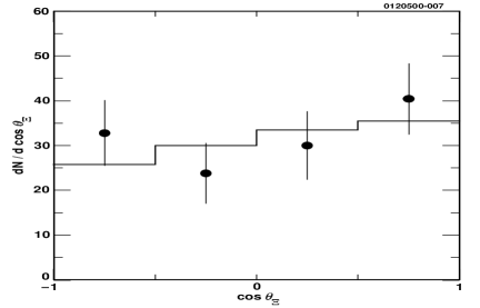
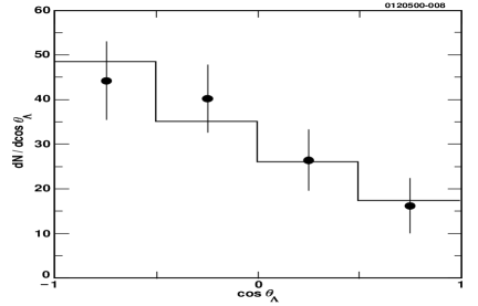
FIG. 3.: Upper plot: the cosine of the angle, $\theta_{\Xi}$, between the $\Lambda$ momentum vector in the $\Xi^{-}$ rest frame and the $\Xi^{-}$ momentum vector in the $\Xi_{c}^{0}$ rest frame, in the decay sequence $\Xi_{c}^{0}\rightarrow\Xi^{-}\pi^{+}$ $\Xi^{-}\rightarrow\Lambda\pi^{-}$, $\Lambda\rightarrow p\pi^{-}$ for sideband subtracted data (points with error bars) and projection of the fit (solid histogram). Lower plot: the cosine of the angle, $\theta_{\Lambda}$, between the proton momentum vector in the $\Lambda$ rest frame and the $\Lambda$ momentum vector in the $\Xi^{-}$ rest frame in the decay sequence $\Xi_{c}^{0}\rightarrow\Xi^{-}\pi^{+}$ $\Xi^{-}\rightarrow\Lambda\pi^{-}$, $\Lambda\rightarrow p\pi^{-}$ for sideband subtracted data (points with error bars) and projection of the fit (solid histogram).

The value of $\alpha_{\Xi}\alpha_{\Lambda}$ found in the fit is in reasonable agreement with a CLEO measurement of $\alpha_{\Xi}\alpha_{\Lambda}=-0.291\pm 0.021\mbox{(stat)}^{+0.019}_{-0.015}\mbox{(syst)}$ obtained with approximately 8,000 $\Xi^{-}\rightarrow\Lambda\pi^{-}$ events [9] and with the current world average value $\alpha_{\Xi}\alpha_{\Lambda}=-0.293\pm 0.007$  [3]. Constraining $\alpha_{\Xi}\alpha_{\Lambda}$ to the world average value does not reduce the statistical error on $\alpha_{\Xi_{c}^{0}}\alpha_{\Xi}$.

We have considered the following sources of systematic error and give our estimate of the percentage error on $\alpha_{\Xi_{c}^{0}}\alpha_{\Xi}$ in parentheses. The statistical error in the MC sample is estimated by varying the size of the MC sample used in the fit $(\pm 2\%)$. The error associated with the uncertainty in the $\Xi_{c}^{0}$ fragmentation function  [10] is estimated by varying this function $(+1\%,-14\%)$. To determine the effect of incomplete knowledge of the background shape and the effect of statistical fluctuations in the sideband sample used to model the background in the signal region, we vary the size of the lower and upper sidebands used in the loglikelihood fit. We also repeat the fit using wrong sign $\Xi^{-}\pi^{-}$ events in both the signal mass region and sideband regions to model the background shape $(+16\%,-1\%)$. The error associated with MC modeling of slow pions from $\Xi$ and $\Lambda$ decay is obtained by varying the reconstruction efficiency according to our understanding of the CLEO II detector $(+9\%,-6\%)$. Using a large sample of $\Xi_{c}^{0}\rightarrow\Xi^{-}\pi^{+}$ MC generated with $\alpha_{\Xi_{c}^{0}}=-0.5$ and the world average values of $\alpha_{\Xi}$ and $\alpha_{\Lambda}$ and including a randomly generated background based on the shape of the data sideband, we measure the effect of varying the size of the area element used to determine $\Gamma_{S}(\cos\theta_{\Xi},\cos\theta_{\Lambda};\alpha_{\Xi_{c}^{0}},\alpha_{\Xi},\alpha_{\Lambda})$ and the background shape $\Gamma_{B}(\cos\theta_{\Xi},\cos\theta_{\Lambda})$ in the loglikelihood fit $(+1\%,-2\%)$. The fit method is checked by integrating over $\cos\theta_{\Lambda}$ ($\cos\theta_{\Xi}$) and performing a one dimensional binned fit to $\cos\theta_{\Xi}$ ($\cos\theta_{\Lambda}$). The results are consistent with the maximum likelihood fit. Possible background from $\Sigma_{c}^{0}(2450)\rightarrow\Lambda_{c}^{+}\pi^{-}_{\rm{slow}}$, $\Lambda_{c}^{+}\rightarrow\Lambda\pi^{+}_{\rm{fast}}$ is determined to be negligible by MC simulation. This measurement is insensitive to production polarization, ${\bf P_{\Xi_{c}^{0}}}$, and no systematic error has been included from this source [12]. Adding all sources of systematic error in quadrature $(+19\%,-15\%)$, we find $\alpha_{\Xi_{c}^{0}}\alpha_{\Xi}=0.26\pm 0.18\mbox{(stat)}^{+0.05}_{-0.04}\mbox{(syst)}$. A similar study for the systematic uncertainty on the measurement of $\alpha_{\Xi}\alpha_{\Lambda}$ in $\Xi_{c}^{0}\rightarrow\Xi^{-}\pi^{+}$ yields $(-8\%,+4\%)$ and consequently $\alpha_{\Xi}\alpha_{\Lambda}=-0.57\pm 0.21\mbox{(stat)}^{+0.05}_{-0.02}\mbox{(syst)}$.

From the measurement of $\alpha_{\Xi_{c}^{0}}\alpha_{\Xi}$ and the PDG evaluation: $\alpha_{\Xi}=-0.456\pm 0.014$  [3], we obtain $\alpha_{\Xi_{c}^{0}}=-0.56\pm 0.39\mbox{(stat)}^{+0.10}_{-0.09}\mbox{(syst)}$. The physically allowed range of a decay asymmetry parameter is $-1<\alpha<+1$. Our result prefers a negative value: $\alpha_{\Xi_{c}^{0}}$ is $<0.1$ at the 90% CL. The central value is in the middle of the theoretically expected range but is not yet precise enough to choose between models.

We note that $\alpha_{\Xi}$ has, so far, always been determined as a product of decay asymmetries using Equation 2. In principle, given sufficient statistics, the loglikelihood method in conjunction with the two-fold joint angular distribution of Equation 4 allows the direct measurement of all three asymmetry parameters: $\alpha_{\Xi_{c}^{0}}$, $\alpha_{\Xi}$, and $\alpha_{\Lambda}$.

In conclusion, from a sample of $138\pm 14$ $\Xi_{c}^{0}\rightarrow\Xi^{-}\pi^{+}$ decays we have measured $\alpha_{\Xi_{c}^{0}}\alpha_{\Xi}=0.26\pm 0.18\mbox{(stat)}^{+0.05}_{-0.04}\mbox{(syst)}$, from which we obtain $\alpha_{\Xi_{c}^{0}}=-0.56\pm 0.39\mbox{(stat)}^{+0.10}_{-0.09}\mbox{(syst)}$. To the best of our knowledge this is the first measurement of a charm strange baryon decay asymmetry parameter.

We gratefully acknowledge the effort of the CESR staff in providing us with excellent luminosity and running conditions. This work was supported by the National Science Foundation, the U.S. Department of Energy, Research Corporation, the Natural Sciences and Engineering Research Council of Canada, the A.P. Sloan Foundation, the Swiss National Science Foundation, and the Alexander von Humboldt Stiftung.

REFERENCES

-
[1]
J.G. Körner, G. Krämer, and J. Wilrodt, Z.
Phys. C 2,
117 (1979).
T.Uppal, R.C. Verma and M.P. Khanna, Phys. Rev. D 49, 3417 (1994).
G. Kaur and M.P. Khanna, Phys Rev. D 44, 182 (1991). Q.P. Xu, and An. N. Kamal, Phys. Rev. D 46, 270 (1992).
P. Żencykowski, Phys. Rev. D 50, 410 (1994).
J.G. Körner and M. Krämer, Z. Phys. C 55, 659 (1992).
H. Cheng and B. Tseng, Phys. Rev. D 46, 1041 (1992). H. Cheng and B. Tseng, Phys. Rev D 48, 4188 (1993). - [2] G. Källen, Elementary Particle Phyics Addison-Wesley, Reading MA, (1964).
- [3] Particle Data Group, Eur. Phys. J. C 15, 1 (2000).
-
[4]
J. Bjorken, Phys. Rev. D 40, 1513 (1989).
T. Mannel, W.Roberts and Z. Ryzak, Phys. Lett. B 225, 593 (1991). - [5] P. Bialas, J.G. Körner M. Krämer and Z. Zalewski, Z. Phys. C 57, 115 (1995), and private communication.
- [6] Y. Kubota et al., Nucl. Instr. and Meth. A 230, 66 (1992).
- [7] GEANT 3.15. R. Brun et al., CERN DD/EE/84-1.
- [8] D.M. Schmidt, R.M. Morrison and M.S. Witherell, Nucl. Inst. and Meth. A 328, 547 (1993).
- [9] CLEO Collaboration, M. Bishai et al., CLEO 98-15 CLNS 98/1587 (1998). Submitted to Physical Review Letters.
- [10] CLEO Collaboration, T. Bergfeld et al., CLEO CONF 97-19 EPS97, 392 (1997).
- [11] C. Peterson, D. Schlatter, I. Schmitt and P.M. Zerwas, Phys. Rev. D 27, 105 (1983).
- [12] Parity conservation in the electromagnetic and strong interactions requires production polarization to be normal to the production plane, and charge conjugation invariance requires the sign of the polarization to be the same for particle and anti-particle. Since is CP-odd, () is CP-odd so that averaged over charge conjugate states the net polarization is zero.