Dalitz Analysis of the Decay $D^{0}\to K^{-}\pi^{+}\pi^{0}$

Abstract

We use data collected with the CLEO II detector to perform a high-statistics measurement of the resonant substructure in $D^{0}\to K^{-}\pi^{+}\pi^{0}$ decays. We find the Dalitz Plot is well represented by a combination of seven quasi-two-body decay channels ($\overline{K}^{*0}\pi^{0}$, $K^{-}\rho$, $K^{*-}\pi^{+}$, $K_{0}(1430)^{-}\pi^{+}$, $\overline{K}_{0}(1430)^{0}\pi^{0}$, $K^{-}\rho^{+}(1700)$, and $K^{*}(1680)^{-}\pi^{+}$), plus a small non-resonant component. We see no evidence of a scalar $\kappa\rightarrow K^{-}\pi^{+}$ resonance in the mass range recently reported by other groups. Using the amplitudes and phases from this analysis, we calculate an integrated CP asymmetry of $-0.031\pm 0.086$.

S. Kopp,¹ M. Kostin,¹ A. H. Mahmood,² S. E. Csorna,³ I. Danko,³ K. W. McLean,³ Z. Xu,³ R. Godang,⁴ G. Bonvicini,⁵ D. Cinabro,⁵ M. Dubrovin,⁵ S. McGee,⁵ G. J. Zhou,⁵ A. Bornheim,⁶ E. Lipeles,⁶ S. P. Pappas,⁶ M. Schmidtler,⁶ A. Shapiro,⁶ W. M. Sun,⁶ A. J. Weinstein,⁶ D. E. Jaffe,⁷ G. Masek,⁷ H. P. Paar,⁷ D. M. Asner,⁸ A. Eppich,⁸ T. S. Hill,⁸ R. J. Morrison,⁸ R. A. Briere,⁹ G. P. Chen,⁹ T. Ferguson,⁹ H. Vogel,⁹ A. Gritsan,¹⁰ J. P. Alexander,¹¹ R. Baker,¹¹ C. Bebek,¹¹ B. E. Berger,¹¹ K. Berkelman,¹¹ F. Blanc,¹¹ V. Boisvert,¹¹ D. G. Cassel,¹¹ P. S. Drell,¹¹ J. E. Duboscq,¹¹ K. M. Ecklund,¹¹ R. Ehrlich,¹¹ A. D. Foland,¹¹ P. Gaidarev,¹¹ L. Gibbons,¹¹ B. Gittelman,¹¹ S. W. Gray,¹¹ D. L. Hartill,¹¹ B. K. Heltsley,¹¹ P. I. Hopman,¹¹ L. Hsu,¹¹ C. D. Jones,¹¹ J. Kandaswamy,¹¹ D. L. Kreinick,¹¹ M. Lohner,¹¹ A. Magerkurth,¹¹ T. O. Meyer,¹¹ N. B. Mistry,¹¹ E. Nordberg,¹¹ M. Palmer,¹¹ J. R. Patterson,¹¹ D. Peterson,¹¹ D. Riley,¹¹ A. Romano,¹¹ J. G. Thayer,¹¹ D. Urner,¹¹ B. Valant-Spaight,¹¹ G. Viehhauser,¹¹ A. Warburton,¹¹ P. Avery,¹² C. Prescott,¹² A. I. Rubiera,¹² H. Stoeck,¹² J. Yelton,¹² G. Brandenburg,¹³ A. Ershov,¹³ D. Y.-J. Kim,¹³ R. Wilson,¹³ T. Bergfeld,¹⁴ B. I. Eisenstein,¹⁴ J. Ernst,¹⁴ G. E. Gladding,¹⁴ G. D. Gollin,¹⁴ R. M. Hans,¹⁴ E. Johnson,¹⁴ I. Karliner,¹⁴ M. A. Marsh,¹⁴ C. Plager,¹⁴ C. Sedlack,¹⁴ M. Selen,¹⁴ J. J. Thaler,¹⁴ J. Williams,¹⁴ K. W. Edwards,¹⁵ R. Janicek,¹⁶ P. M. Patel,¹⁶ A. J. Sadoff,¹⁷ R. Ammar,¹⁸ A. Bean,¹⁸ D. Besson,¹⁸ X. Zhao,¹⁸ S. Anderson,¹⁹ V. V. Frolov,¹⁹ Y. Kubota,¹⁹ S. J. Lee,¹⁹ R. Mahapatra,¹⁹ J. J. O’Neill,¹⁹ R. Poling,¹⁹ T. Riehle,¹⁹ A. Smith,¹⁹ C. J. Stepaniak,¹⁹ J. Urheim,¹⁹ S. Ahmed,²⁰ M. S. Alam,²⁰ S. B. Athar,²⁰ L. Jian,²⁰ L. Ling,²⁰ M. Saleem,²⁰ S. Timm,²⁰ F. Wappler,²⁰ A. Anastassov,²¹ E. Eckhart,²¹ K. K. Gan,²¹ C. Gwon,²¹ T. Hart,²¹ K. Honscheid,²¹ D. Hufnagel,²¹ H. Kagan,²¹ R. Kass,²¹ T. K. Pedlar,²¹ H. Schwarthoff,²¹ J. B. Thayer,²¹ E. von Toerne,²¹ M. M. Zoeller,²¹ S. J. Richichi,²² H. Severini,²² P. Skubic,²² A. Undrus,²² V. Savinov,²³ S. Chen,²⁴ J. Fast,²⁴ J. W. Hinson,²⁴ J. Lee,²⁴ D. H. Miller,²⁴ E. I. Shibata,²⁴ I. P. J. Shipsey,²⁴ V. Pavlunin,²⁴ D. Cronin-Hennessy,²⁵ A.L. Lyon,²⁵ E. H. Thorndike,²⁵ T. E. Coan,²⁶ V. Fadeyev,²⁶ Y. S. Gao,²⁶ Y. Maravin,²⁶ I. Narsky,²⁶ R. Stroynowski,²⁶ J. Ye,²⁶ T. Wlodek,²⁶ M. Artuso,²⁷ R. Ayad,²⁷ C. Boulahouache,²⁷ K. Bukin,²⁷ E. Dambasuren,²⁷ G. Majumder,²⁷ G. C. Moneti,²⁷ R. Mountain,²⁷ S. Schuh,²⁷ T. Skwarnicki,²⁷ S. Stone,²⁷ J.C. Wang,²⁷ A. Wolf,²⁷ and J. Wu²⁷

I Introduction

A clearer understanding of final state interactions in exclusive weak decays is an important ingredient for our ability to model decay rates as well as for our understanding of interesting phenomena such as mixing [1]. There are several theoretical methods  [2, 3, 4, 5, 6] used to understand the dynamics of two body charmed meson decays with experimental measurements as input. Unfortunately, final-state interactions are often not well understood, and may not be included properly in many models. These long-distance strong interaction effects can cause significant changes in decay rates for specific final states, and can cause shifts in the phases of the decay amplitudes.

Three-body decays provide a rich laboratory in which to study the interference between intermediate state resonances, and provide a direct probe of the final state interactions in certain decays. When a particle decays into three or more daughters, intermediate resonances dominate the decay rate. These resonances will cause a non-uniform distribution of events in phase space when analyzed using a “Dalitz Plot” technique [7]. Since all events of a particular decay mode have the same final state, multiple resonances at the same location in phase space will interfere. This provides the opportunity to experimentally measure both the amplitudes and phases of the intermediate decay channels, which in turn allows us to deduce their relative branching fractions. These phase differences can even allow details about very broad resonances to be extracted by observing their interference with other intermediate states.

This paper describes a study of the underlying structure in $D^{0}\to K^{-}\pi^{+}\pi^{0}$ decays [14]. Four previous groups have made similar measurements, each with less than 1000 signal events[8, 9, 10, 11]. In addition to significantly increasing our statistical power, the large CLEO II dataset on which this analysis is based also permits us to tighten analysis requirements to drastically reduce the effect of backgrounds. Coupled with the superb resolution of the CLEO-II detector, this has allowed us to extract significantly more information about this decay than was possible in the past.

II Theoretical Models

Since we are studying the decay of a spin-zero particle to three daughters, only two degrees-of-freedom are required to completely describe the kinematics. To see this, consider the decay in the $D^{0}$ rest frame. The four-momenta of the three final state particles correspond to twelve unknowns. We have one constraint for each known mass and four additional constraints from the conservation of momentum and energy in the decay. Finally, since the three degrees of freedom describing the spatial orientation of the decay are irrelevant (the $D^{0}$ having spin zero) only two independent degrees of freedom remain.

There are three invariant masses that can be formed by considering all possible pairs of final state particles: $M^{2}_{K^{-}\pi^{+}}$, $M^{2}_{K^{-}\pi^{0}}$ and $M^{2}_{\pi^{+}\pi^{0}}$. Only two of these are independent, however, since energy and momentum conservation results in the additional constraint

$$M^{2}_{D^{0}}+M^{2}_{K^{-}}+M^{2}_{\pi^{+}}+M^{2}_{\pi^{0}}=M^{2}_{K^{-}\pi^{+}}+M^{2}_{K^{-}\pi^{0}}+M^{2}_{\pi^{+}\pi^{0}}.$$ (1)

Choosing two of the above three invariant masses as dynamic variables has two compelling advantages: i) Their relativistic invariance means the Lorentz frame in which they are evaluated is irrelevant; ii) As the expression for the partial width in Equation 2 indicates, we expect that a scatter plot of events in the $M_{12}^{2}$ vs $M_{23}^{2}$ plane (known as a Dalitz Plot) will be uniformly distributed if phase-space alone determines the decay dynamics. This allows the decay fraction at each point to be readily correlated with the decay matrix element $\cal M$ without additional corrections:

$$d\Gamma={|{\cal M}|^{2}\over{256\pi^{3}M_{D}^{3}}}dM_{12}^{2}dM_{23}^{2}.$$ (2)

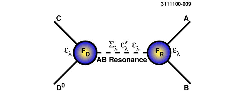
FIG. 1.: A Representation of the three body decay of $D^{0}\to ABC$ through an AB resonance. The spin sum is performed to obtain the angular dependence of the decay.

In this analysis we choose $M^{2}_{K^{-}\pi^{+}}$ and $M^{2}_{\pi^{+}\pi^{0}}$ as our two Dalitz Plot variables, and must next construct the relevant decay amplitudes in terms of these. The dynamics can be understood with the aid of Figure 1. We first consider the decay of the $D^{0}$ meson into particle C plus an AB resonance, followed by the decay of the AB resonance into particles A and B. To properly describe the structure of this decay using our Dalitz Plot variables, we need to obtain the angular dependence of the decay products. Each vertex in Figure 1 contains a spin factor $\varepsilon_{\lambda}$ which depends on the type of the decay: scalar, vector, tensor, etc. The matrix element for a vector decay is

$${\cal M}=F_{D}(P_{D^{0}}+P_{C})_{\mu}{\sum_{\lambda}\varepsilon^{\mu*}_{\lambda}\varepsilon^{\nu}_{\lambda}\over{M^{2}_{r}-M^{2}_{AB}-iM_{r}\Gamma_{AB}}}(P_{A}-P_{B})_{\nu}F_{r}$$ (3)

where $P$ denotes 4-momentum, and $M_{r}$ is the mass of the resonance. In general the form factors at each vertex, $F_{D}$ and $F_{r}$, are unknown functions, however in practice they are either set to a constant value or to the Blatt-Weisskopf penetration factors [12].

The spin-sum in the numerator of Equation 3 is evaluated to give

$$\sum_{\lambda}\varepsilon^{\mu*}_{\lambda}\varepsilon^{\nu}_{\lambda}=-g^{\mu\nu}+{{P_{AB}^{\mu}P_{AB}^{\nu}}\over{M_{AB}^{2}}}$$ (4)

and the “mass dependent width” $\Gamma_{AB}$ is a function of the AB invariant mass $M_{AB}$, the momentum of either daughter in the AB rest frame $p_{AB}$, the momentum of either daughter in the resonance rest frame $p_{r}$, the spin of the resonance $J$, the width of the resonance $\Gamma_{r}$, and is expressed as [13]:

$$\Gamma_{AB}=\Gamma_{r}\left(p_{AB}\over{p_{r}}\right)^{2J+1}\left(M_{r}\over{M_{AB}}\right)F_{r}^{2}$$ (5)

We relax the transversality requirement on the vector resonance in Equation 4 and divide by $M_{r}^{2}$ instead of $M_{AB}^{2}$. This substitution gives rise to a small spin zero component when the vector resonance is off mass-shell, a behavior which is observed to occur with the $W$ boson and which should also be expected in the resonance behavior we are studying here.

Inserting this expression for the spin-sum into Equation 3 and summing over the repeated indices gives the Lorentz invariant expression for the matrix element of a vector particle as a function of position in the Dalitz Plot:

$${\cal A}_{1}(ABC|r)=F_{D}F_{r}{M^{2}_{AC}-M^{2}_{BC}+{(M^{2}_{D}-M^{2}_{C})(M^{2}_{B}-M^{2}_{A})\over{M^{2}_{r}}}\over{M^{2}_{r}-M^{2}_{AB}-iM_{r}\Gamma_{AB}}}.$$ (6)

The procedure for calculating the vector matrix element is generalizable to intermediate particles having other spin. For example, we can easily find the amplitude for a spin zero resonance to be

$${\cal A}_{0}(ABC|r)=F_{D}F_{r}{1\over{M^{2}_{r}-M^{2}_{AB}-iM_{r}\Gamma_{AB}}}.$$ (7)

The procedure for higher spin resonances involves a bit more algebra. For example, the spin two case starts with

$${\cal A}_{2}(ABC|r)=F_{D}(P_{D}+P_{C})_{\mu}(P_{D}+P_{C})_{\nu}{\sum_{\lambda}\varepsilon^{\mu\nu*}_{\lambda}\varepsilon^{\alpha\beta}_{\lambda}\over{M^{2}_{r}-M^{2}_{AB}-iM_{r}\Gamma_{AB}}}(P_{A}-P_{B})_{\alpha}(P_{A}-P_{B})_{\beta}F_{r}.$$ (8)

In this case the spin sum has been previously calculated by Pilkuhn [13] to be

$$\sum\limits_{\lambda}{\varepsilon_{\lambda}^{*\mu\nu}\varepsilon_{\lambda}^{\alpha\beta}}=\frac{1}{2}\left({T^{\mu\alpha}T^{\nu\beta}+T^{\mu\beta}T^{\nu\alpha}}\right)-\frac{1}{3}T^{\mu\nu}T^{\alpha\beta}$$ (9)

where

$$T^{\mu\nu}=-g^{\mu\nu}+{{P^{\mu}P^{\nu}}\over{M^{2}}}$$ (10)

When this expression is inserted into Equation 8 and the implied sums performed we find the final form of the tensor matrix element:

$${\cal A}_{2}(ABC|r)={F_{D}F_{r}\over{M_{r}^{2}-M^{2}_{AB}-i\Gamma_{AB}M_{r}}}\left[\left(M^{2}_{BC}-M^{2}_{AC}+{(M_{D}^{2}-M_{C}^{2})(M_{A}^{2}-M_{B}^{2})\over{M_{r}^{2}}}\right)^{2}\right.$$

$$-\frac{1}{3}\left(M^{2}_{AB}-2M_{D}^{2}-2M_{C}^{2}+{(M_{D}^{2}-M_{C}^{2})^{2}\over{M_{r}^{2}}}\right)\left.\left(M^{2}_{AB}-2M_{A}^{2}-2M_{B}^{2}+{(M^{2}_{A}-M^{2}_{B})^{2}\over{M_{r}^{2}}}\right)\right].$$ (11)

Next we return to the form factors $F_{D}$ and $F_{r}$, which attempt to model the underlying quark structure of the $D^{0}$ meson and the intermediate resonances. We use the Blatt-Weisskopf penetration factors shown in Table I. These have one free parameter, R, which is the “radius” of the meson, and are dependent on the momentum $P$ of the decay particles in the parent rest frame. In all cases, we normalize the form factor to have unit value at the nominal meson mass. The fits display very little sensitivity to the meson radii; good fits are obtained when these values vary between $0\ {\rm GeV}^{-1}$ and $10\ {\rm GeV}^{-1}$ for the $D^{0}$ and between $0\ {\rm GeV}^{-1}$ and $3\ {\rm GeV}^{-1}$ for the intermediate resonances. To be consistent with other experiments [8] we have chosen the $D^{0}$ to have $R=5\ {\rm GeV}^{-1}$ and the intermediate resonances all to have $R=1.5\ {\rm GeV}^{-1}$

TABLE I.: Blatt-Weisskopf Penetration Form Factors. $p_{r}$ is the momentum of either daughter in the meson rest frame. $p_{AB}$ is the momentum of either daughter in the candidate rest frame (same as $p_{r}$ except the parent mass used is the two-track invariant mass of the candidate rather than the mass of the meson). $R$ is the meson radial parameter.

Spin	Form Factor $F_{r}$
0	1
1	${\sqrt{1+R^{2}p^{2}_{r}}\over{\sqrt{1+R^{2}p^{2}_{AB}}}}$
2	${\sqrt{9+3R^{2}p^{2}_{r}+R^{4}p^{4}_{r}}\over{\sqrt{9+3R^{2}p^{2}_{AB}+R^{4}p^{4}_{AB}}}}$

Before continuing, we must specify our phase conventions for the intermediate resonances. We can explicitly see the importance of specifying the ordering of particles in the decay by examining Equation 6. If we were to switch the labels A and B we would generate an overall minus sign causing the phase to change by 180^o. In an attempt to be consistent with previous results we have chosen the phases in the same way as the E687 collaboration [8] since they are the only group to have explicitly published their choice of phases and matrix elements.

Now that we know the form of the intermediate resonance amplitudes, and have chosen a phase convention that will allow us to compare our results with previous measurements, we can write down an expression for the overall matrix element of the decay. Guided by the results of previous measurements [8, 9, 10], we begin with only three vector resonances $\rho(770)^{+}$, $K^{*-}$ and $\bar{K}^{*0}$ [15] as well as a flat non-resonant (nr) component:

$${\cal M}(D^{0}\to K^{-}\pi^{+}\pi^{0}) = a_{nr}e^{i\phi_{nr}}$$ (15)

$$+a_{\rho}e^{i\phi_{\rho}}{\cal A}_{1}(\pi^{+}\pi^{0}K^{-}|\rho^{+})$$

$$+a_{\bar{K}^{*0}}e^{i\phi_{\bar{K}^{*0}}}{\cal A}_{1}(K^{-}\pi^{+}\pi^{0}|\bar{K}^{*0})$$

$$+a_{K^{*-}}e^{i\phi_{K^{*-}}}{\cal A}_{1}(K^{-}\pi^{0}\pi^{+}|K^{*-}),$$

where the $a_{i}$ and $\phi_{i}$ are the amplitude and relative phase of the $i$’th component respectively. The overall normalization is arbitrary, and is chosen to be

$$\int|{\cal M}|^{2}d{\cal DP}=1$$ (16)

where $d{\cal DP}$ indicates that the integral is performed over the Dalitz Plot. This is equivalent to saying that we are sensitive only to relative phases and amplitudes, which in turn means that we are free to fix one phase and one amplitude in Equation 15. To minimize correlated errors on the phases and amplitudes we choose the largest mode, $K^{-}\rho$, to have a fixed zero phase and an amplitude of one.

Since the choice of normalization, phase convention, and amplitude formalism may not always be identical for different experiments, fit fractions are reported instead of amplitudes to allow for more meaningful comparisons between results. The fit fraction is defined as the integral of a single component divided by the coherent sum of all components:

$${\rm Fit\ Fraction}={\int\left|a_{r}e^{i\phi_{r}}{\cal A}(ABC|r)\right|^{2}d{\cal DP}\over{\int\left|\sum_{j}a_{j}e^{i\phi_{j}}{\cal A}(ABC|j)\right|^{2}d{\cal DP}}}.$$ (17)

The sum of the fit fractions for all components of a fit will in general not be one because of interference.

One must also consider the statistical errors on the fit fractions. We have chosen to use the full covariance matrix from the fits to determine the errors on fit fractions so that the assigned errors will properly include the correlated components of the errors on the amplitudes and phases. After each fit, the covariance matrix and final parameter values are used to generate 500 sample parameter sets. For each set, the fit fractions are calculated and recorded in histograms. Each histogram is fit with a single Gaussian to extract its width, which is used as a measure of the statistical error on the fit fraction.

III Experimental Details

The CLEO II detector is described elsewhere [16]. This measurement uses the entire CLEO II dataset, which represents approximately $4.7$ fb^-1 of integrated $e^{+}e^{-}$ luminosity at $\sqrt{s}\sim 10.6$ GeV.

The $D^{0}$’s used in this analysis are required to be produced by the decay chain $D^{*+}\to D^{0}\pi^{+}_{s}$, which significantly reduces the combinatorial background. To reconstruct the $D^{0}$’s, we take pairs of oppositely charged tracks and assign the track with the same sign as the pion from the $D^{*+}$ decay to be the pion from the $D^{0}$ decay. This Cabibbo-favored correlation between the signs of the pions eliminates the need for other particle identification techniques in this analysis.

For tracks to be used they must be well fitted, reconstruct to within 5 cm of the interaction point along the beam pipe and within 5 mm perpendicular to the beam pipe (corresponding to about 5 standard deviations in length and more than 10 standard deviations in the width of the beam spot).

We fit pairs of tracks passing these requirements to a common vertex, which is the candidate decay position of the $D^{0}$ meson. Each such pair of charged tracks is combined with all $\pi^{0}$ candidates in an event. The $\pi^{0}$ candidates are found by combining all pairs of electromagnetic showers which are unmatched to charged tracks. To reduce the number of fake $\pi^{0}$’s from random shower combinations and to improve their resolution, we require that each shower have energy above 100 MeV and be in the central region of the CLEO II detector. Furthermore, the invariant mass of the two photon combination is restricted to be between 128 MeV/c²and 140 MeV/c²(i.e. within about one standard deviation of the $\pi^{0}$ mass). The two shower combination is kinematically fit to give the known $\pi^{0}$ mass.

Once we have a vertex with a $K^{-}$, a $\pi^{+}$ and a $\pi^{0}$ candidate, we combine the momenta of the three particles to find the $D^{0}$ momentum. With the decay location and the momentum known, the $D^{0}$ is projected back to the beam spot. In CLEO, the beam spot has a ribbon like shape with a width of 700 $\mu$m, a height of 20 $\mu$m, and a length of about 2 cm. We project the $D^{0}$ candidate back to the vertical position of the beam, since this dimension of the beam is most precisely known. The intersection of the $D^{0}$ projection and the beam position defines the production point of the $D^{*+}$.

We refit the slow pion track to include the $D^{*+}$ production point as an additional constraint, providing a better measurement of its true momentum. The result of this is that the width of the mass difference peak, $\Delta M=M(D^{*+})-M(D^{0})$, is reduced from 590 keV to 490 keV, providing a 15% reduction in the number of background events in our final sample. We make a requirement that $\Delta M$ is between 144.9 MeV/c²and 145.9 MeV/c². We also require that the normalized $D^{*}$ momentum, $X_{D^{*}}={P_{D^{*}}/\sqrt{E^{2}_{beam}-M^{2}_{D^{*}}}}$, is greater than 0.6, which significantly reduces the combinatorial background level and kinematically excludes the possibility that a $D^{*}$ candidate came from a decaying $B$ meson.

After obtaining the candidate $D^{0}$’s as described above, we can plot the mass of the $D^{0}\to K^{-}\pi^{+}\pi^{0}$ candidates as shown in Figure 2, where the fit to the mass distribution is also shown. When examining the Dalitz Plot, we only use the events which have $1.85\,{\rm GeV/c}^{2}<M_{D^{0}}<1.88\,{\rm GeV/c}^{2}$ (i.e. within about one standard deviation of the known $D^{0}$ mass).

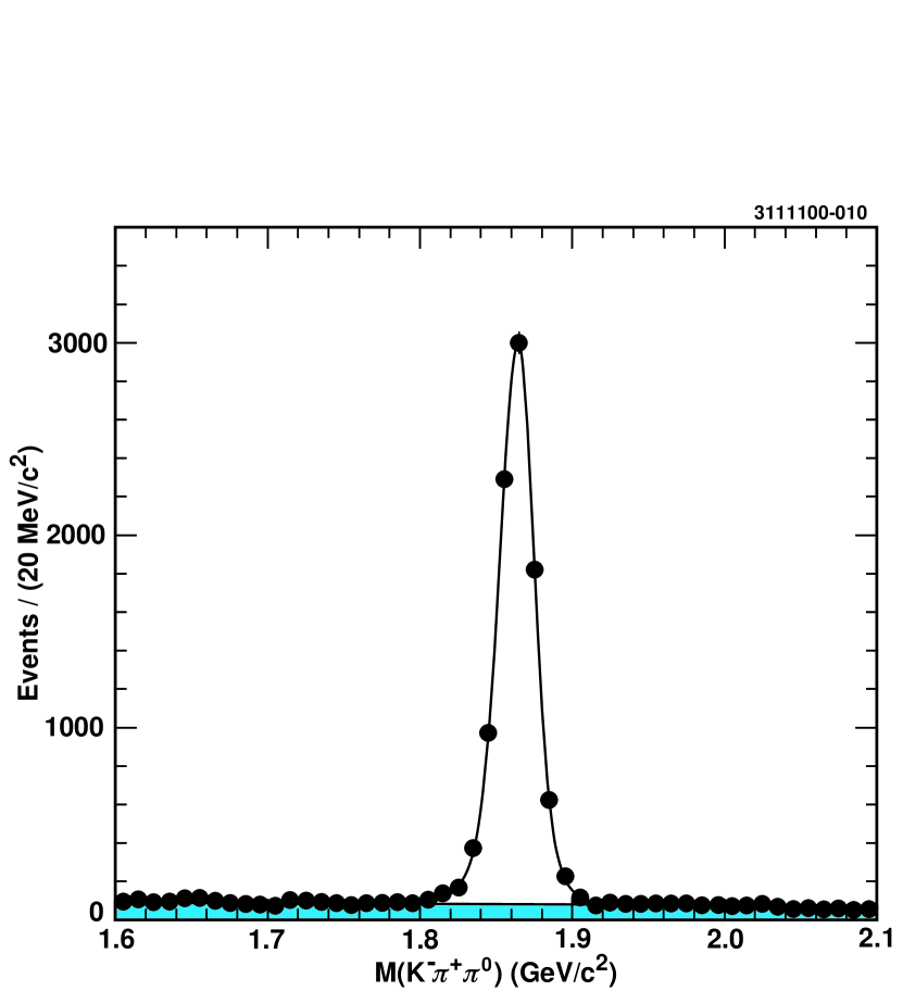
FIG. 2.: The $D^{0}\to K^{-}\pi^{+}\pi^{0}$ reconstructed mass distribution for all event candidates (points). The solid line represents a fit to the data using a double bifurcated Gaussian to represent the signal plus a straight line to represent the background (shaded).

We have chosen quite restrictive cuts on our kinematic variables (approximately one standard deviation on each) to minimize the effect of the background on our result. Since we are studying the shape of the distribution and are not trying to extract a branching ratio, the fact that this increases the systematic uncertainty of the overall efficiency somewhat is not an issue.

Applying the above requirements produces 7,070 events in the Dalitz Plot. Figure 3 shows the distribution of this sample as a scatter plot in the chosen mass squared variables $M_{K^{-}\pi^{+}}^{2}$ and $M_{\pi^{+}\pi^{0}}^{2}$.

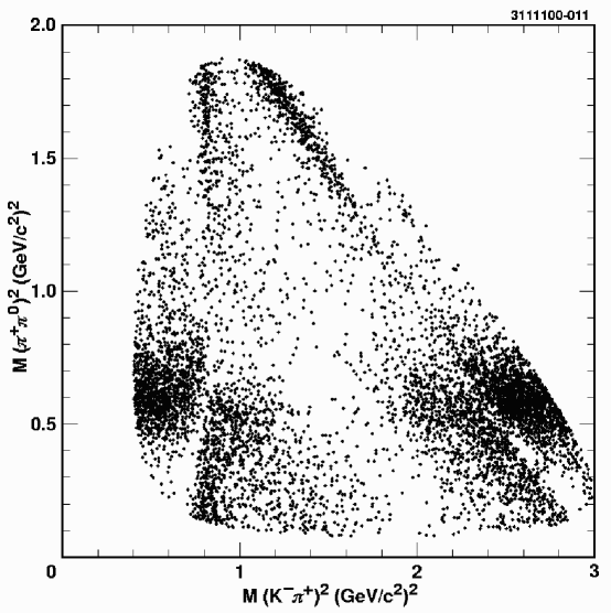
FIG. 3.: The Dalitz distribution of all 7,070 $D^{0}\to K^{-}\pi^{+}\pi^{0}$ candidates in our data sample shown in an unbinned scatter plot.

In order to reduce the smearing effects introduced by the detector, those combinations passing the above requirements are kinematically fit such that when combined, the $K^{-}$, $\pi^{+}$ and $\pi^{0}$ reconstruct to give the correct $D^{0}$ mass. This kinematic fit has two effects. First, the uncertainty of the 4-momentum of the particles is reduced, giving a more precise measurement of the mass squared variables used to define an event’s position in the Dalitz Plot. Second, the decay position in these variables is guaranteed to respect the kinematic boundaries of the Dalitz Plot.

A Background

Turning again to Figure 2, we can see that the signal region contains a small but non-zero number of background events. We use the fit shown to measure the fraction of events in this region which are “true signal” by integrating the signal function (a double bifurcated Gaussian) and the background function (a line) and comparing the two. The signal fraction and its associated statistical error, $0.967\pm 0.011$, are used in the likelihood function minimized during the fitting procedure.

Knowing only the amount of background is not enough if we want to correctly extract the amplitudes and phases of the signal component; the shape of the background in the Dalitz Plot is also important. There are several sidebands [17] that could be chosen to study the shape of this background using data, and a Monte Carlo study (outlined below) is used to determine which one is best. As will become apparent in the section on systematic errors, the overall low level of the background means that the final result has very little sensitivity to this choice.

To determine which sideband will best represent the Dalitz Plot shape of the background in the signal region, a signal-free sample of $e^{+}e^{-}\rightarrow q\overline{q}$ Monte Carlo simulated data is used (referred to below as the “vetoed” sample). These data are generated using a full GEANT based detector simulation [18], and are processed by the same reconstruction code that is used for real data.

This Monte Carlo sample represents the background we want to measure in data, and we use it as a reference in our study. The next step is to consider a number of possible sideband samples, and see which does the best job representing the Dalitz shape of the vetoed sample.

Many sideband samples can be formed in the space defined by the three mass variables, $\Delta M$, $M_{D^{0}}$ and $M_{\pi^{0}}$. To choose the best one, we fit the distribution in the Dalitz Plot using an unbinned likelihood fit to a cubic polynomial in $M^{2}_{K^{-}\pi^{+}}$ and $M^{2}_{\pi^{+}\pi^{0}}$ as well as non-interfering squared amplitudes for the $\rho(770)$, $K^{*}(892)^{-}$ and $\overline{K}^{*0}$. A $\chi^{2}$ is formed between each Monte Carlo sideband sample and the reference vetoed sample to give us a measure of their relative merits.

Based on this, the sideband which seems to best represent the vetoed sample consists of those events which have $\Delta M<0.1549$ GeV/c², are in the $M_{\pi^{0}}$ signal region, and are in the off-peak regions of $M_{D^{0}}$: $1.76<M_{D^{0}}{\rm(GeV/c^{2})}<1.80$ or $1.91<M_{D^{0}}{\rm(GeV/c^{2})}<1.95$. This choice of sidebands along with the $D^{0}\to K^{-}\pi^{+}\pi^{0}$ candidates are shown in Figure 4.

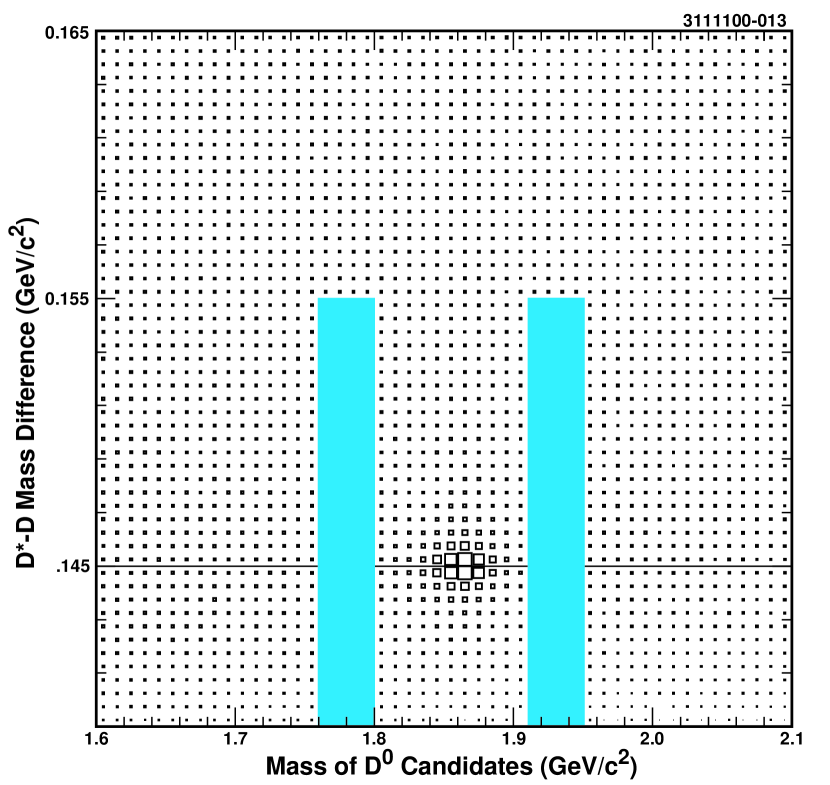
FIG. 4.: A box plot showing $D^{0}\to K^{-}\pi^{+}\pi^{0}$ candidates in the $\Delta M$ vs $M_{D^{0}}$ plane. The shaded areas on each side of the peak are the sidebands determined to best represent the background.

The assumption is now made that the sideband method which best represents the background in the Dalitz Plot when analyzing the Monte Carlo simulated data is also the best sideband method for use in real data. Those events from the actual data which are in the selected “best” sideband are fit with the cubic polynomial plus the three non-interfering resonances. The resulting best fit parameters are shown in Table II. We project the fit and the background points onto the three mass squared variables and show the results in Figure 5, along with a two dimensional Manhattan plot of the fit result. We use this parameterization of the background shape in the fit to the distribution of events in the Dalitz Plot by including both the parameters and the covariance matrix in the final likelihood function (as described in Section IV).

TABLE II.: Background and efficiency best fit parameters. The fitting functions are described in Section IV.

Background		Efficiency
$B_{0}$	$1.0$ (fixed)	$E_{0}$	$(22.1\pm 1.8)\times 10^{-5}$
$B_{x}$	$-1.188\pm 0.018$	$E_{x}$	$(-6.89\pm 2.9)\times 10^{-5}$
$B_{y}$	$-0.742\pm 0.044$	$E_{y}$	$(-27.1\pm 3.7)\times 10^{-5}$
$B_{x^{2}}$	$0.483\pm 0.015$	$E_{x^{2}}$	$(10.4\pm 1.6)\times 10^{-5}$
$B_{xy}$	$0.874\pm 0.032$	$E_{xy}$	$(38.2\pm 3.2)\times 10^{-5}$
$B_{y^{2}}$	$0.122\pm 0.047$	$E_{y^{2}}$	$(12.4\pm 2.8)\times 10^{-5}$
$B_{x^{3}}$	$-0.052\pm 0.004$	$E_{x^{3}}$	$(-3.00\pm 0.27)\times 10^{-5}$
$B_{x^{2}y}$	$-0.162\pm 0.010$	$E_{x^{2}y}$	$(-7.97\pm 0.73)\times 10^{-5}$
$B_{xy^{2}}$	$-0.202\pm 0.014$	$E_{xy^{2}}$	$(-12.8\pm 0.94)\times 10^{-5}$
$B_{y^{3}}$	$0.061\pm 0.016$	$E_{y^{3}}$	$(-0.53\pm 0.73)\times 10^{-5}$
$B_{\overline{K}^{*0}}$	$(1.65\pm 1.70)\times 10^{-5}$
$B_{\rho^{+}}$	$(3.69\pm 0.58)\times 10^{-4}$
$B_{K^{*-}}$	$(7.69\pm 1.95)\times 10^{-5}$

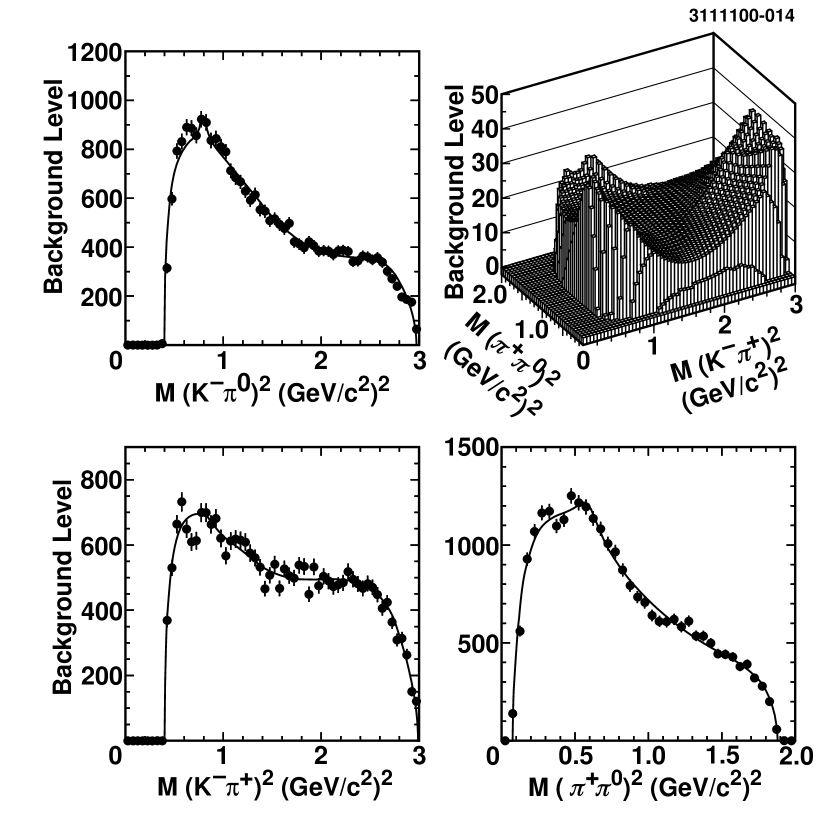
FIG. 5.: Results of the best fit to the $D^{0}\to K^{-}\pi^{+}\pi^{0}$ sideband background sample. The fit function is shown as a Manhattan plot (top right), and as projections onto the three mass squared variables showing both fit (histogram) and data (points).

B Efficiency

Next, we determine the efficiency for detecting signal events as a function of position in the two dimensional Dalitz Plot. After generating 4.2 million signal Monte Carlo events with a flat distribution in phase space (i.e., uniform across the Dalitz Plot), these events are analyzed to find the number of observed events as a function of $M^{2}_{K^{-}\pi^{+}}$ and $M^{2}_{\pi^{+}\pi^{0}}$. The events observed are binned into regions with $50~{}({\rm MeV/c}^{2})^{2}$ on a side, and we divide the number of events observed in each bin by the number generated to give a measure of the efficiency for that bin. Due to the finite number of Monte Carlo events observed in each bin, each individual efficiency measurement has about a 10% statistical error. Since we expect (and observe) that the efficiency is a slowly varying function across the Dalitz Plot, we fit the efficiency measurements with a cubic polynomial in $M^{2}_{K^{-}\pi^{+}}$ and $M^{2}_{\pi^{+}\pi^{0}}$ and use the resulting function to parameterize the efficiency.

As a check that the efficiency function obtained using phase space Monte Carlo is reasonable, we repeat the procedure described above with another 2.4 million signal Monte Carlo events generated with the Dalitz distribution found by E691 [9]. Again the efficiency in each bin is calculated and fit. Since the resulting fit agrees well with the efficiency calculated from the phase space distribution of points, we combine the two Monte Carlo samples and calculate the efficiency using the full 6.6 million events. The fit parameters for this combined fit are shown in Table II. Figure 6 shows the raw efficiency for each bin as well as the fit and the projections onto each of the three mass-squared axes.

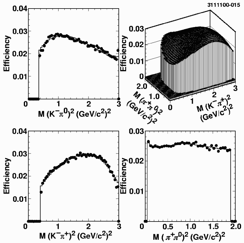
FIG. 6.: Results of the best fit to the $D^{0}\to K^{-}\pi^{+}\pi^{0}$ detection efficiency distribution. The fit function is shown as a Manhattan plot (top right), and as projections onto the three mass squared variables of both fit (histogram) and raw efficiency (points). In each of the projections, the quantity plotted is the average efficiency at the given $M^{2}$ value.

IV Fitting Procedure

Having a parameterization for both the background and efficiency as well as knowing the fraction of events in the signal region which are in fact background, we can fit the data in the Dalitz Plot to extract the amplitudes and phases of any contributing intermediate resonances.

To do this we use an unbinned maximum likelihood fit which minimizes the function ${\cal F}$ given by

$${\cal F}={\big{[}\sum_{events}-2\ln{\cal L}\big{]}+\chi^{2}_{\rm penalty}}$$ (18)

where

$${\cal L}=\left({F{{\cal E}(M^{2}_{K^{-}\pi^{+}},M^{2}_{\pi^{+}\pi^{0}})\left|{\cal M}\right|^{2}}\over{{\cal N}_{signal}}}+(1-F){{{\cal B}(M^{2}_{K^{-}\pi^{+}},M^{2}_{\pi^{+}\pi^{0}})}\over{{\cal N}_{background}}}\right)$$ (19)

$$\chi^{2}_{\rm penalty} =\left({F-F_{o}\over{\sigma_{F}}}\right)^{2}+\sum_{ij}(B_{i}-B_{io})V_{ij}(B_{j}-B_{jo})$$ (20)

$$+E_{sys}\sum_{ij}(E_{i}-E_{io})W_{ij}(E_{j}-E_{jo})$$ (21)

and

$${\cal N}_{signal}=\int{{\cal E}(M^{2}_{K^{-}\pi^{+}},M^{2}_{\pi^{+}\pi^{0}})\left|{\cal M}\right|^{2}}d{\cal DP}$$ (22)

$${\cal N}_{background}=\int{\cal B}(M^{2}_{K^{-}\pi^{+}},M^{2}_{\pi^{+}\pi^{0}})d{\cal DP}.$$ (23)

The signal fraction $F_{o}$ and its error $\sigma_{F}$ (0.967 and 0.011 respectively) are determined from the fit to the $D^{0}$ mass spectrum shown in Figure 2, and the the parameters $B_{jo}$ and $E_{jo}$ describe the nominal background and efficiency shapes (see Table II) via the cubic polynomial shapes

$${\cal B} = B_{0}+B_{x}M^{2}_{K^{-}\pi^{+}}+B_{y}M^{2}_{\pi^{+}\pi^{0}}+B_{x^{2}}(M^{2}_{K^{-}\pi^{+}})^{2}+B_{xy}M^{2}_{K^{-}\pi^{+}}M^{2}_{\pi^{+}\pi^{0}}+B_{y^{2}}(M^{2}_{\pi^{+}\pi^{0}})^{2}+$$ (26)

$$B_{x^{3}}(M^{2}_{K^{-}\pi^{+}})^{3}+B_{x^{2}y}(M^{2}_{K^{-}\pi^{+}})^{2}M^{2}_{\pi^{+}\pi^{0}}+B_{xy^{2}}M^{2}_{K^{-}\pi^{+}}(M^{2}_{\pi^{+}\pi^{0}})^{2}+B_{y^{3}}(M^{2}_{\pi^{+}\pi^{0}})^{3}+$$

$$B_{\overline{K}^{*0}}|{\cal A}_{1}(K^{-}\pi^{+}\pi^{0}|\overline{K}^{*0})|^{2}+\beta_{\rho}|{\cal A}_{1}(\pi^{+}\pi^{0}K^{-}|\rho^{+})|^{2}+\beta_{K^{*-}}|{\cal A}_{1}(K^{-}\pi^{0}\pi^{+}|K^{*-})|^{2}$$

and

$${\cal E} = E_{0}+E_{x}M^{2}_{K^{-}\pi^{+}}+E_{y}M^{2}_{\pi^{+}\pi^{0}}+E_{x^{2}}(M^{2}_{K^{-}\pi^{+}})^{2}+E_{xy}M^{2}_{K^{-}\pi^{+}}M^{2}_{\pi^{+}\pi^{0}}+E_{y^{2}}(M^{2}_{\pi^{+}\pi^{0}})^{2}+$$ (28)

$$E_{x^{3}}(M^{2}_{K^{-}\pi^{+}})^{3}+E_{x^{2}y}(M^{2}_{K^{-}\pi^{+}})^{2}M^{2}_{\pi^{+}\pi^{0}}+E_{xy^{2}}M^{2}_{K^{-}\pi^{+}}(M^{2}_{\pi^{+}\pi^{0}})^{2}+E_{y^{3}}(M^{2}_{\pi^{+}\pi^{0}})^{3}$$

.

In expressing this likelihood function we have made the explicit assumption that background events and signal events are distinct, allowing us to factor the likelihood into two components which do not interfere. The $\chi^{2}_{\rm penalty}$ terms represent the information from the fits used to determine the signal fraction, the background parameterization, and the efficiency parameterization. $V_{ij}$ and $W_{ij}$ are the covariance matrices from the background and efficiency fits respectively. The last term is used only when evaluating the systematic errors due to the efficiency parameterization, hence $E_{sys}$ is set to zero during “normal” fitting.

In addition to the likelihood, we need a measure to assess how well any given fit represents the data. A confidence level can be calculated directly from the likelihood function by utilizing the best fit parameters. This idea was described by ARGUS [20] and is a direct application of the Central Limit Theorem from statistics [21]. Assuming the candidates are truly distributed according to the likelihood function which gives the best fit, the average value is

$$\mu=\frac{1}{N}\sum_{i=1}^{N}(-2\ln{\cal L})\approx\int{\cal L}(-2\ln{\cal L})d{\cal DP}$$ (29)

where $N$ is the number of candidates. The variance is given by

$$\sigma^{2}_{\mu}=\frac{1}{N}\sum_{i=1}^{N}(-2\ln{\cal L}-\mu)^{2}\approx\int{\cal L}(-2\ln{\cal L})^{2}d{\cal DP}-\mu^{2}.$$ (30)

Because we have a large number of candidates distributed according to this function, the Central Limit Theorem tells us that the mean should follow a normal distribution. The sum of minus log likelihoods, which is the value minimized in the fit, has a mean of $N\mu$ and follows a normal distribution with a variance of $N\sigma^{2}_{\mu}$. Thus, the minimal value will come from a normal distribution with mean

$$<-2\sum\ln{\cal L}>=N\int{\cal L}(-2\ln{\cal L})d{\cal DP}-n$$ (31)

and standard deviation

$$\sigma_{<-2\sum\ln{\cal L}>}=\sqrt{N\int{\cal L}(-2\ln{\cal L})^{2}d{\cal DP}-N\mu^{2}}$$ (32)

where $n$ is the number of parameters extracted from the fit. The confidence level for the fit is then just the area of a Gaussian with the above mean and width which lies above the value obtained in our fit. It is worth pointing out that this value only gives a measurement of the goodness of fit assuming the fit function correctly describes the true distribution.

Having a second measure of the goodness of the fit would be extremely valuable, and an obvious choice is the $\chi^{2}$. This requires the data to be binned, and furthermore that there are enough events in each bin that Gaussian statistics can be assumed. As we saw in Figure 3, the density of candidates in the $D^{0}\to K^{-}\pi^{+}\pi^{0}$ Dalitz Plot varies significantly as a function of position, hence to form a sensible $\chi^{2}$ measure we will need to have bins of varying size.

To systematically choose these bins, we start by placing a grid of small regions, $50~{}({\rm MeV/c}^{2})^{2}$ on a side, over the Dalitz Plot. Next, adjacent regions are combined into bins until each contains approximately 30 candidates. After completing this procedure, our Dalitz Plot is divided into 228 bins of varying size, and a $\chi^{2}$ variable for the multinomial distribution [22, 23] can be calculated as

$$\chi^{2}=-2\sum_{i=1}^{228}n_{i}\ln\left(\frac{p_{i}}{n_{i}}\right)$$ (33)

where $n_{i}$ is the number of events observed in bin $i$, and $p_{i}$ is the number predicted from the fit. For a large number of events this formulation of the $\chi^{2}$ becomes equivalent to the usual one [24].

One can naively calculate the number of degrees of freedom for the fit as the number of bins (r) minus the number of fit parameters (k) minus one, as would be correct for a binned maximum likelihood fit. However, since we are minimizing the unbinned likelihood function, our “$\chi^{2}$” variable does not asymptotically follow a $\chi^{2}$ distribution [24], but it is bounded by a $\chi^{2}$ variable with $(r-1)$ degrees of freedom and a $\chi^{2}$ variable with $(r-k-1)$ degrees of freedom. Because it is bounded by two $\chi^{2}$ variables, it should be a useful statistic for comparing the relative goodness of fits. In what follows, we use both the $\chi^{2}$ and the confidence level described above as our “goodness of fit” measures to determine which of the many possible sets of intermediate resonances are preferred.

Before analyzing the $D^{0}\to K^{-}\pi^{+}\pi^{0}$ data, we performed many checks of both the fitting and fit evaluation procedures. One of these was a double-blind study in which several Monte Carlo samples containing $D^{0}\to K^{-}\pi^{+}\pi^{0}$ decays generated with “secret” mixtures of intermediate resonances were analyzed. In each case, our fitting and evaluation procedure identified the correct set of resonances, and recovered their amplitudes and phases within statistical errors. The resulting amplitudes and phases for one of the fits is shown in Table III.

TABLE III.: A comparison between input Monte Carlo parameters and the results from a subsequent fit to the Dalitz Plot using the techniques described in Section IV. Note that the input amplitudes and phases are completely fictitious.

Resonance	Generated		Measured
	Amplitude	Phase (degrees)	Amplitude	Phase (degrees)
$\overline{K}^{*0}$	1.0	45	$1.03\pm 0.02$	$47\pm 1$
$\rho^{+}$	1.0	0	$1.0$ (fixed)	$0$ (fixed)
$K^{*-}$	1.0	-115	$1.03\pm 0.02$	$-113\pm 2$
$K^{*}_{0}(1430)^{-}$	0.5	-115	$0.54\pm 0.05$	$-107\pm 6$
Non resonant	1.0	-90	$1.08\pm 0.05$	$273\pm 3$

V Fitting the Data

Armed with the tools described in the previous section, we are ready to fit the data distribution shown in Figure 3. Previous experiments have observed three intermediate resonances in $D^{0}\to K^{-}\pi^{+}\pi^{0}$ decays: $\rho^{+}$, $\overline{K}^{*0}$ and $K^{*-}$, hence we begin by considering only these in addition to a non-resonant component. The resulting fit parameters are given in Table IV.

TABLE IV.: Results of the best fit to the data with only $\rho^{+}$, $\overline{K}^{*0}$, $K^{*-}$, and non-resonant components included.

	$a_{nr}$			$1.70\pm 0.07$
	$a_{\rho^{+}}$			$1.00$ (fixed)
	$a_{K^{*-}}$			$0.378\pm 0.008$
	$a_{\overline{K}^{*0}}$			$0.422\pm 0.009$
	$\phi_{nr}$			$59.7^{o}\pm 2.0^{o}$
	$\phi_{\rho^{+}}$			$0^{o}$ (fixed)
	$\phi_{K^{*-}}$			$166.7\pm 2.0^{o}$
	$\phi_{\overline{K}^{*0}}$			$-7.8^{o}\pm 2.2^{o}$
	$-2\ln{\cal L}$			7070
	Conf. Level.			0.0%
	$\chi^{2}$			650

Figure 7 shows the projections of both the fit and the data onto the three mass squared variables, as well as a two dimensional Manhattan plot of the final fit function. Even a quick glance suggests that the data is not well represented by this function, and the large value of $\chi^{2}$ as well as the zero confidence level confirm this observation. These parameters are useful for comparison with previous experiments, however, which reported observation of these three resonances with much less statistics. We show the comparison in Tables V and VI and see good agreement. Unfortunately, we can only compare the results for the phases to E687 since the other experiments do not give their choice of particle ordering or potential complex constants in their choice for ${\cal A}(ABC|r)$. Although the phases match for the three resonant components, the non-resonant phase seems to be off by 180^o. This observation is consistent with comments that E687 had an unreported negative sign in their vector amplitude [25].

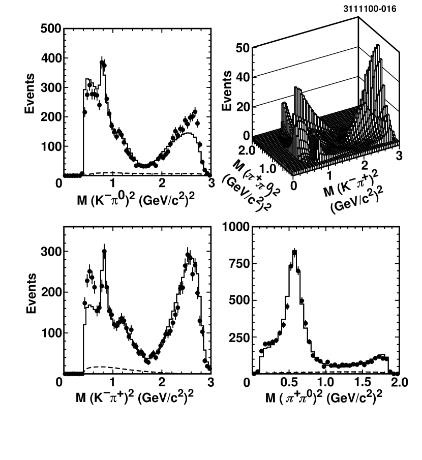
FIG. 7.: The results of fitting the $D^{0}\to K^{-}\pi^{+}\pi^{0}$ data with only $\rho^{+}$, $\overline{K}^{*0}$, $K^{*-}$, and non resonant components included. The efficiency corrected fit is shown as a Manhattan plot (top right), and as projections onto the three mass squared variables of both fit (histogram) and data (points). The dashed line shows the level of the background.

TABLE V.: A comparison of the fit fractions obtained with our “three resonance” fit and those reported by previous experiments. The errors shown are statistical only. Note that although the data is not well fit by this model, the results are consistent with those reported by previous experiments.

Decay Mode	CLEO II (3 Resonance)	E687	Mark III	E691
$K^{-}\rho^{+}$	$0.834\pm 0.007$	$0.765\pm 0.041$	$0.81\pm 0.03$	$0.647\pm 0.039$
$K^{*-}\pi^{+}$	$0.129\pm 0.006$	$0.148\pm 0.028$	$0.12\pm 0.02$	$0.084\pm 0.011$
$\overline{K}^{*0}\pi^{0}$	$0.157\pm 0.007$	$0.165\pm 0.031$	$0.13\pm 0.02$	$0.142\pm 0.018$
Non resonant	$0.074\pm 0.006$	$0.101\pm 0.033$	$0.09\pm 0.02$	$0.036$

TABLE VI.: A comparison of the phases (in degrees) obtained with our “three resonance” fit and those reported by previous experiments. The errors shown are statistical only. In the “Rotated” column we have shifted the reported phases such that the $\rho$ has a phase of $0^{o}$ in order to ease comparison with the other results. Note that although the data is not well fit by this model, the results are consistent with those reported by previous experiments.

Decay Mode	CLEO II (3 Resonance)	E687	Mark III	E691 (Rotated)
$K^{-}\rho^{+}$	$0$ (fixed)	$0$ (fixed)	$0$ (fixed)	$0\pm 7$
$K^{*-}\pi^{+}$	$166.7\pm 2.0$	$162\pm 10$	$154\pm 11$	$-152\pm 9$
$\overline{K}^{*0}\pi^{0}$	$-7.8\pm 2.2$	$-2\pm 12$	$7\pm 7$	$127\pm 9$
Non-resonant	$59.7\pm 2.0$	$-122\pm 10$	$52\pm 9$	$-40$ (fixed)

Since we have at least a factor of ten more statistics for this analysis, one should not be surprised that more resonances are needed to accurately represent the data. The question now becomes how best to determine which additional resonances to include. We have tried two procedures: a) adding all possible resonances and subsequently removing those which do not contribute significantly, and b) adding new resonances one at a time and choosing the best additional one at each iteration, stopping when no additional resonances contribute significantly. Both of these methods lead us to the same results, hence only the first one is described below.

We begin by fitting the Dalitz Plot with all known resonances which can possibly contribute to this decay, as listed in Table VII [26]. The results of this fit are shown in the “All Resonances” column of Table VIII, and in Figure 8. There are five resonances which have fit fractions that are less than one standard deviation away from zero: $\overline{K}^{*}_{3}(1780)^{0}$, $K^{*}_{3}(1780)^{-}$, $\overline{K}^{*}(1410)^{0}$, $K^{*}(1410)^{-}$ and $\overline{K}^{*}(1680)^{0}$. Two other resonances, $\overline{K}^{*}_{2}(1430)^{0}$ and $K^{*}_{2}(1430)^{-}$, have fit fractions close to zero. When the first five resonances are removed and the fit repeated, the fit fractions of these last two resonances do become consistent with zero, and hence are also removed.

TABLE VII.: The resonances considered when fitting the $D^{0}\to K^{-}\pi^{+}\pi^{0}$ Dalitz Plot, along with the masses and widths used when evaluating the matrix element.

	Parameters
Resonance	$J^{P}$	Mass (GeV/c2)	Width (GeV/c2)
$\rho(770)^{+}$	$1^{-}$	$0.770\pm 0.001$	$0.1507\pm 0.0011$
$\overline{K}^{*}(892)^{0}$	$1^{-}$	$0.8961\pm 0.0003$	$0.0505\pm 0.0006$
$K^{*}(892)^{-}$	$1^{-}$	$0.8915\pm 0.0003$	$0.050\pm 0.001$
$K^{*}(1410)^{-}$	$1^{-}$	$1.414\pm 0.015$	$0.232\pm 0.021$
$\overline{K}^{*}(1410)^{0}$	$1^{-}$	$1.414\pm 0.015$	$0.232\pm 0.021$
$K^{*}_{0}(1430)^{-}$	$0^{+}$	$1.412\pm 0.006$	$0.294\pm 0.023$
$\overline{K}^{*}_{0}(1430)^{0}$	$0^{+}$	$1.412\pm 0.006$	$0.294\pm 0.023$
$K^{*}_{2}(1430)^{-}$	$2^{+}$	$1.425\pm 0.002$	$0.098\pm 0.003$
$\overline{K}^{*}_{2}(1430)^{0}$	$2^{+}$	$1.432\pm 0.001$	$0.109\pm 0.005$
$\rho(1450)^{+}$	$1^{-}$	$1.465\pm 0.025$	$0.310\pm 0.060$
$\rho(1700)^{+}$	$1^{-}$	$1.700\pm 0.020$	$0.240\pm 0.060$
$K^{*}(1680)^{-}$	$1^{-}$	$1.717\pm 0.027$	$0.322\pm 0.110$
$\overline{K}^{*}(1680)^{0}$	$1^{-}$	$1.717\pm 0.027$	$0.322\pm 0.110$
$\overline{K}^{*}_{3}(1780)^{0}$	$3^{-}$	$1.776\pm 0.007$	$0.159\pm 0.021$
$K^{*}_{3}(1780)^{-}$	$3^{-}$	$1.776\pm 0.007$	$0.159\pm 0.021$

FIG. 8.: The results of fitting the $D^{0}\to K^{-}\pi^{+}\pi^{0}$ data with all known resonances likely to contribute (see Table VII). The efficiency corrected fit is shown as a Manhattan plot (top right), and as projections onto the three mass squared variables of both fit (histogram) and data (points). The dashed line shows the level of the background.

TABLE VIII.: The parameters from the fits to the $D^{0}\to K^{-}\pi^{+}\pi^{0}$ Dalitz Plot with all resonances included (“All Resonances” column), and after we remove resonances consistent with zero fit fraction (“Final Resonances” column). The $\rho(1450)^{+}$ and $\rho(1700)^{+}$ contributions are discussed in the text.

	All Resonances		Final Resonances
Component	Phase (degrees)	Fit Fraction (%)	Phase (degrees)	Fit Fraction (%)
$\overline{K}_{3}(1780)^{0}$	$263\pm 16$	$0.3\pm 7.5$
$K_{3}(1780)^{-}$	$86\pm 12$	$0.5\pm 2.9$
$\overline{K}^{*}(1680)^{0}$	$175\pm 25$	$0.4\pm 0.5$
$K^{*}(1680)^{-}$	$67\pm 19$	$1.0\pm 0.5$	$103\pm 8$	$1.3\pm 0.3$
$\rho(1700)^{+}$	$149\pm 8$	$75\pm 18$	$171\pm 6$	$5.7\pm 0.8$
$\rho(1450)^{+}$	$-45\pm 10$	$34\pm 11$
Non Res.	$30\pm 5$	$9.1\pm 1.3$	$31\pm 4$	$7.5\pm 0.9$
$\overline{K}^{*}(1410)^{0}$	$279\pm 52$	$0.1\pm 0.2$
$\overline{K}_{2}(1430)^{0}$	$148\pm 13$	$0.3\pm 0.14$
$\overline{K}_{0}(1430)^{0}$	$168\pm 5$	$8.0\pm 1.3$	$166\pm 5$	$4.1\pm 0.6$
$K^{*}(1410)^{-}$	$152\pm 31$	$0.2\pm 0.2$
$K_{2}(1430)^{-}$	$339\pm 21$	$0.12\pm 0.08$
$K_{0}(1430)^{-}$	$42\pm 6$	$5.6\pm 1.1$	$55.5\pm 5.8$	$3.3\pm 0.6$
$K^{*}(892)^{-}$	$159\pm 2.6$	$12.8\pm 1.8$	$163\pm 2.3$	$16.1\pm 0.7$
$\rho(770)^{+}$	$0$(fixed)	$74\pm 4$	$0$ (fixed)	$78.7\pm 2.0$
$\overline{K}^{*}(892)^{0}$	$2.8\pm 3.2$	$11.3\pm 1.5$	$-0.2\pm 3.3$	$12.7\pm 0.9$
$\chi^{2}$	203		257
$-2\ln{\cal L}$	6490		6570
C.L.	91.3		94.9

Notice that in the “All Resonances” column of Table VIII there are two heavy $\rho$ mesons ($\rho(1450)^{+}$ and $\rho(1700)^{+}$) which have surprisingly large fit fractions. Both have masses which place their peak outside the Dalitz Plot, but both are wide enough ($310\pm 60$ MeV/c² and $240\pm 60$ MeV/c² respectively [26]) that their tails extend well into the region of interest, making it difficult to distinguish between them. Since the fitted phases of these $\rho$’s are very close to being $180^{o}$ apart, their large fit fractions are assumed to be an artifact of the fit’s inability to tell them apart. Supporting this is the additional fact that when both resonances are combined, their net contribution to the fit fraction is much smaller, $(9\pm 2)\%$. Since the inclusion of both $\rho$ resonances is probably a misrepresentation of the contents of the Dalitz Plot, only one of these is included in all following fits. We choose the one which gives the best $\chi^{2}$ and goodness of fit, the $\rho(1700)^{+}$, and consider the $\rho(1450)^{+}$ only when evaluating our systematic errors.

After the seven resonances consistent with zero fit fraction are removed along with the $\rho(1450)^{+}$ (as discussed above), seven resonances remain in addition to the non-resonant component: $\rho(770)^{+}$, $K^{*}(892)^{-}$, $\overline{K}^{*}(892)^{0}$, $\rho(1700)^{+}$, $\overline{K}_{0}(1430)^{0}$, $K_{0}(1430)^{-}$, and $K^{*}(1680)^{-}$. Figure 9 shows the result of fitting the Dalitz Plot with these components. The fit fractions and phases are shown in the “Final Resonances” column of Table VIII, and the full set of parameters extracted from this fit is shown in Table IX.

TABLE IX.: Summary of our best fit to the data with the final set of eight components included.

Signal Parameters						Background Parameters
	$a_{nr}$			$1.75\pm 0.12$
	$a_{\rho^{+}}$			$1.00$ (fixed)			$B_{0}$			$1.0\pm 0.0$
	$a_{K^{*-}}$			$0.44\pm 0.01$			$B_{x}$			$-1.206\pm 0.001$
	$a_{\overline{K}^{*0}}$			$0.39\pm 0.01$			$B_{y}$			$-0.74\pm 0.23$
	$a_{K_{0}(1430)^{-}}$			$0.77\pm 0.08$			$B_{x^{2}}$			$0.468\pm 0.001$
	$a_{\overline{K}_{0}(1430)^{0}}$			$0.85\pm 0.06$			$B_{xy}$			$0.842\pm 0.008$
	$a_{\rho(1700)^{+}}$			$2.50\pm 0.19$			$B_{y^{2}}$			$0.168\pm 0.001$
	$a_{K^{*}(1680)^{-}}$			$2.50\pm 0.3$			$B_{x^{3}}$			$-0.055\pm 0.001$
	$\phi_{NR}$			$31.2^{o}\pm 4.3^{o}$			$B_{x^{2}y}$			$-0.16\pm 0.06$
	$\phi_{\rho^{+}}$			$0^{o}$ (fixed)			$B_{xy^{2}}$			$-0.188\pm 0.001$
	$\phi_{K^{*-}}$			$163\pm 2.3^{o}$			$B_{y^{3}}$			$0.077\pm 0.001$
	$\phi_{\overline{K}^{*0}}$			$-0.2^{o}\pm 3.3^{o}$			$B_{\overline{K}^{*0}}$			$(3.4\pm 0.1)\times 10^{-5}$
	$\phi_{K_{0}(1430)^{-}}$			$55.5^{o}\pm 5.8^{o}$			$B_{\rho}$			$(4.27\pm 0.05)\times 10^{-4}$
	$\phi_{\overline{K}_{0}(1430)^{0}}$			$166^{o}\pm 5^{o}$			$B_{K^{*-}}$			$(9.64\pm 0.01)\times 10^{-5}$
	$\phi_{\rho(1700)^{+}}$			$171^{o}\pm 6^{o}$
	$\phi_{K^{*}(1680)^{-}}$			$103^{o}\pm 8^{o}$
	Signal Fraction			$0.968\pm 0.007$
	$-2\ln{\cal L}$			6570
	Conf. Level.			94.9%
	$\chi^{2}$			257

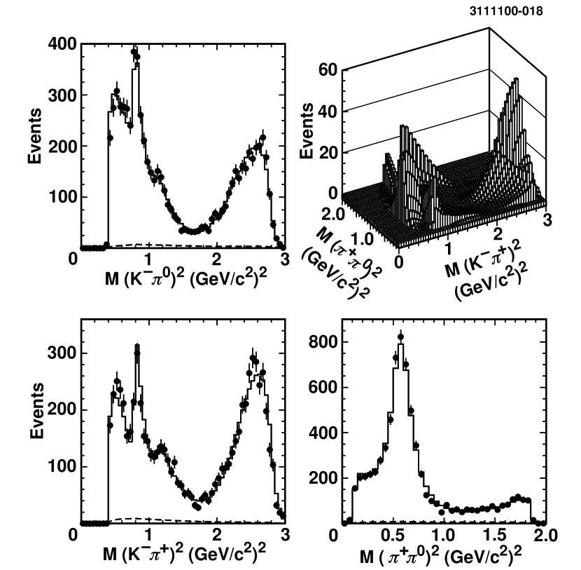
FIG. 9.: The results of fitting the $D^{0}\to K^{-}\pi^{+}\pi^{0}$ data with the “final set” of components. The efficiency corrected fit is shown as a Manhattan plot (top right), and as projections onto the three mass squared variables of both fit (histogram) and data (points). The dashed line shows the level of the background.

As a curious side note, if a single vector ($K^{-}\pi^{0}$) resonance with a floating mass and width is added in place of the four new “standard resonances” discussed above, a good fit can obtained. Unfortunately, while this new resonance has a reasonable mass of 1.406 GeV/c², it prefers a negative width of $\Gamma=-0.25$ GeV/c² which does not seem to represent the underlying dynamics we are trying to measure. It is possible that the desire for this resonance is an indication of an inaccuracy of the formalism used for the resonance shapes, or an indication that multiple resonances are needed (as we have assumed). We note that the optimum set of seven resonances used above, all of which have positive widths, provide a fit which has a lower $\chi^{2}$ than the inclusion of this single unphysical state.

Other experiments have reported evidence of a light scalar ($\pi^{+}\pi^{-}$) resonance, the $\sigma$, in $D^{+}\rightarrow\pi^{-}\pi^{+}\pi^{+}$ decays [28], as well as evidence of a scalar ($K^{-}\pi^{+}$) resonance, the $\kappa$, in $D^{+}\rightarrow K^{-}\pi^{+}\pi^{+}$ decays  [29]. Since a significant fit fraction for $D^{+}\rightarrow\kappa\pi^{+}$ has been reported by these authors, we have searched for a scalar $\kappa\rightarrow K^{-}\pi^{+}$ resonance in the $D^{0}\rightarrow\kappa\pi^{0}$ channel, fixing the mass and width of the $\kappa$ to the values reported in [29], (0.815 GeV/c²  and 0.560 GeV/c²  respectively). We find a fit fraction consistent with zero ($0.4\pm 0.3$%), and see no improvement in the confidence level of the fit with this additional resonance included. We have also allowed the mass and width of the $\kappa$ to float in the fit, and again see no significant contribution.

Lastly, since this analysis considers only $D^{0}$ mesons produced from a decaying $D^{*+}$ in the mode $D^{*+}\to D^{0}\pi^{+}_{s}$, we have the ability to divide our data into separate $D^{0}$ and $\overline{D^{0}}$ samples by simply considering the sign of the $\pi^{\pm}_{s}$ from the $D^{*\pm}$ decay. The Dalitz Plots of these samples can then be fitted separately and compared in a search for CP violation. We have fitted these samples with the same set of resonances described above, and the results are shown in Table X. When performing these fits, the efficiency functions were found separately for the $D^{0}$ and $\overline{D^{0}}$ samples, however a common background shape was assumed. Forming a simple $\chi^{2}$ between the two sets of fit parameters we find $\chi^{2}_{cp}=16.2$ for 14 degrees of freedom.

We calculate an integrated CP asymmetry across the Dalitz Plot by evaluating

$${\cal A}_{cp}=\int{|{\cal M}_{D^{0}}|^{2}-|{\cal M}_{\overline{D^{0}}}|^{2}\over{|{\cal M}_{D^{0}}|^{2}+|{\cal M}_{\overline{D^{0}}}|^{2}}}d{\cal DP}$$ (34)

and obtain ${\cal A}_{cp}=-0.031\pm 0.086$, consistent with zero. Note that this number is not dependent on the number of $D^{0}$ and $\overline{D^{0}}$ candidates in our data sample, but rather on the shapes of these distributions in the respective Dalitz Plots.

TABLE X.: Fit results when the $D^{0}$ and $\overline{D^{0}}$ samples are considered separately.

	$D^{0}$ Sample		$\overline{D^{0}}$ Sample
Component	Amplitude	Phase (degrees)	Amplitude	Phase (degrees)
$\rho(770)^{+}$	$1.0\pm 0.0$	$0^{o}$(fixed)	$1.0\pm 0.0$	$0^{o}$(fixed)
$K^{*}(892)^{-}$	$0.433\pm 0.034$	$168.9\pm 3.3$	$0.442\pm 0.015$	$157.8\pm 3.4$
$\overline{K}^{*}(892)^{0}$	$0.391\pm 0.026$	$1.3\pm 3.7$	$0.410\pm 0.022$	$-4.9\pm 4.9$
$\rho(1700)^{+}$	$2.590\pm 0.538$	$175.0\pm 7.5$	$2.720\pm 0.272$	$163.9\pm 7.6$
$\overline{K}_{0}(1430)^{0}$	$0.989\pm 0.124$	$173.9\pm 8.2$	$0.774\pm 0.089$	$159.3\pm 8.1$
$K_{0}(1430)^{-}$	$0.701\pm 0.211$	$59.0\pm 10.0$	$0.917\pm 0.117$	$55.0\pm 7.1$
$K^{*}(1680)^{-}$	$2.567\pm 1.540$	$107.4\pm 69.2$	$2.060\pm 0.423$	$106.4\pm 13.5$
Non Res.	$1.840\pm 0.146$	$39.9\pm 7.9$	$1.780\pm 0.160$	$21.3\pm 6.0$
$\chi^{2}$	227		233
$-2\ln{\cal L}$	3237		3302
C.L.(%)	93.1		80.7

VI Systematic Uncertainties

After finding the best fit to the data, we must attempt to estimate the systematic uncertainties on the fit parameters. There are several possible sources: the background, the efficiency, biases due to experimental resolution, and the modeling of the decay. These contributions are discussed in order, and the final systematic errors are shown in Table XI, where experimental and model dependent sources of systematic uncertainty are summarized in detail.

The background was modeled by the choice of sideband sample that gave the best parameterization of the vetoed data sample from Monte Carlo. Furthermore, the background parameters were allowed to float in our fits to the data, constrained only by the covariance matrix from the fit that determined the nominal background function. To search for any systematic effects due the background parameterization, the fitting procedure was repeated for a number of different sideband choices. Because the background fraction our sample is a mere 3.3%, or about 230 out of the 7070 events in the Dalitz plot, these changes have a minimal effect on the fit parameters. We use the RMS spread of these results as our estimate of the systematic error due to our choice of background parameterization. These values are shown in the “Bkgnd” column of Table XI.

To obtain the efficiency across the Dalitz Plot, signal Monte Carlo events were fit to a cubic polynomial. As a check, we have allowed this polynomial to float in our fit (as was done with the background) subject to a $\chi^{2}$ constraint from its covariance matrix in the likelihood function (i.e. setting $E_{sys}=1$ in Equation 20). If the efficiency is not well modeled by a cubic polynomial, there could still be an effect that this check would fail to find. To search for this we tried a local smoothing algorithm rather than the global polynomial fit. The efficiency was smoothed by fitting either nine or twenty-five neighbors around each bin with a local plane. Each bin’s efficiency value was then replaced by the height of this plane interpolated to its center. As a final check, we used the raw measurements of the efficiency in each bin of our fits. We conclude that the effects of parameterization of the efficiency function over the Dalitz Plot is not a significant source of concern as most of the fit parameters vary by less than their one sigma error bars in the above checks.

Since we make no requirement on the momentum of the charged tracks, one might worry that low momentum tracks may be poorly measured and could affect the Dalitz Plot distribution in a way not well modeled by our Monte Carlo. To search for such a momentum dependent effect, we fit the data with the additional requirement that all tracks have a momentum above 350 MeV/c.

The cuts used to obtain our signal determine the structure of our efficiency. To assess how well the Monte Carlo reproduces the data distributions, we varied the cuts used in the analysis and fit the resulting Dalitz distributions. Each cut was relaxed in turn. The cuts on the masses, $M_{D^{0}}$, $\Delta M$ and $M_{\pi^{0}}$, were opened to double the size of the signal region. The minimum energy on the photons was relaxed to 90 MeV, and the requirement on $X_{D^{*}}$ was loosened to 0.5.

The RMS variation in the fit parameters from each of the tests described above was taken as our estimate of the systematic uncertainty on the efficiency. These values are shown in the “Eff” column of Table XI.

A final contribution to the experimental systematic error, presented in column “Resol” of Table XI, is due to the finite resolution of the Dalitz Plot variables. As a check, we have included the effects of smearing when fitting the data. This was done by measuring the resolution as a function of position across the Dalitz plot and numerically convoluting this with the amplitude at each point when performing the fit. Again, the parameters vary by less than the statistical errors on the nominal best fit, and their variation from the nominal values is taken as an estimate of the systematic uncertainty.

The above three systematic error categories (background, efficiency and resolution) are summarized in Table XI. They are combined in quadrature to give the total experimental uncertainty, which is shown in the “Total” column under “Experiment”.

TABLE XI.: A summary of the systematic errors on each fit parameter. The first two columns show the results from the best fit and the associated statistical errors. The next four (three) columns summarize the systematic uncertainties due to experimental (modeling) sources respectively. Details are provided in the text.

	From Fit		Experimental Errors				Modeling Errors
Parameter	Value	Stat Err	Bkgnd	Eff	Resol	Total	Shape	Add	Total
$\overline{K}^{*}(892)^{0}$ Fit Frac ($\%$)	12.66	0.91	0.17	0.40	0.24	0.50	1.42	0.38	1.47
$\overline{K}^{*}(892)^{0}$ Phase (deg.)	-0.20	3.28	1.06	1.62	1.04	2.20	6.99	0.67	7.02
$\rho(770)^{+}$ Fit Frac ($\%$)	78.76	1.93	0.52	1.10	0.53	1.33	4.40	1.33	4.60
$K^{*}(892)^{-}$ Fit Frac ($\%$)	16.11	0.69	0.47	0.53	0.18	0.73	${}^{+2.58}_{-0.48}$	0.59	${}^{+2.65}_{-0.76}$
$K^{*}(892)^{-}$ Phase (deg.)	163.40	2.32	0.94	2.62	1.30	3.08	4.20	1.09	4.34
$K_{0}(1430)^{-}$ Fit Frac ($\%$)	3.32	0.64	0.13	0.60	0.40	0.73	1.16	0.40	1.23
$K_{0}(1430)^{-}$ Phase (deg.)	55.52	5.76	1.20	2.76	1.31	3.28	${}^{-12.8}_{+3.1}$	2.85	${}^{+4.2}_{-13.1}$
$\overline{K}_{0}(1430)^{0}$ Fit Frac ($\%$)	4.05	0.61	0.15	0.66	0.24	0.72	${}^{+3.04}_{-0.24}$	0.39	${}^{+3.06}_{-0.46}$
$\overline{K}_{0}(1430)^{0}$ Phase (deg.)	165.90	5.23	2.39	3.83	0.70	4.57	11.4	3.20	11.8
$\rho(1700)^{+}$ Fit Frac ($\%$)	5.65	0.76	0.20	0.43	0.50	0.68	5.71	0.59	5.74
$\rho(1700)^{+}$ Phase (deg.)	170.50	6.07	1.90	3.90	1.50	4.59	${}^{-54.7}_{+3.3}$	5.17	${}^{+6.1}_{-54.9}$
$K^{*}(1680)^{-}$ Fit Frac ($\%$)	1.33	0.33	0.07	0.32	0.11	0.34	0.17	0.32	0.36
$K^{*}(1680)^{-}$ Phase (deg.)	103.20	7.90	3.71	5.91	2.00	7.26	9.21	9.89	13.5
Non Res Fit Frac ($\%$)	7.50	0.95	0.35	0.42	0.05	0.55	${}^{+5.54}_{-0.79}$	0.41	${}^{+5.56}_{-0.89}$
Non Res Phase (deg.)	31.20	4.28	1.28	5.08	1.70	5.51	${}^{-14.4}_{+3.5}$	1.19	${}^{+3.7}_{-14.4}$

Modeling systematic errors can arise from our choice of resonances and the uncertainty in their shapes. In Section II we motivated our choice of parameterization of the intermediate resonances; however, other groups have used different functional forms in their fits [8, 9]. We varied these shapes to study any systematic effects resulting from our choice. We examine three variations: (i) the Zemach formalism [30] which enforces the transversality of the mesons by using $M_{AB}^{2}$ rather than $M_{r}^{2}$ in the denominator of the spin sums, (ii) a simple cosine distribution for the spin sum and (iii) a non-relativistic rather than relativistic Breit-Wigner in the propagator. Further consideration was also given to the radial parameters used in the form factors, which were varied between $0\ {\rm GeV}^{-1}$ and $3\ {\rm GeV}^{-1}$ for the intermediate resonances and between $0\ {\rm GeV}^{-1}$ and $10\ {\rm GeV}^{-1}$ for the $D^{0}$ meson. The masses and widths of the intermediate resonances were allowed to vary within the known errors [26]. The non-resonant contribution was described in our fits by a constant term, but as a check we also modeled it by a linear function or a shape given by the spin structure without the Breit-Wigner amplitudes [31].

The above tests were used to explore the systematic dependance of the fit parameters on the way the physics was modeled. The variations using a simple cosine distribution in place of the spin sum and using a spin structured rather than constant non-resonant component resulted in fits with significantly worsened $\chi^{2}$ (368 and 322 respectively), and are not considered when assigning a systematic error as the data suggests these forms could not be correct. We take the largest of the remaining variations as the systematic error due to our choice of modeling shapes, and the results are shown in the “Shape” column of Table XI.

The final systematic check is on our choice of which resonances to include. For example, there is only a slight preference for the $\rho(1700)^{+}$ over the $\rho(1450)^{+}$ based on the goodness of fit. To account for this uncertainty, both fits were performed and the variation of the parameters were noted. Fits were also performed which included additional resonances from Table VII. The RMS variation in the fit parameters from the above checks is presented in the “Add” column of Table XI.

We also considered the effects of removing resonances, and two of these studies deserve further comment. The first is the removal of the $K^{*}(1680)^{-}$. We considered this because the final fit fraction for this resonance is a rather small $1.3\pm 0.3$%. When the $K^{*}(1680)^{-}$ is removed the $\chi^{2}$ increases from 257 to 316 indicating that this resonance should remain. The parameters for this fit are shown in the “Removed $K^{*}(1680)^{-}$” column of Table XII. For comparison, when the other “new” resonances, $\overline{K}_{0}(1430)^{0}$, $K_{0}(1430)^{-}$, and $\rho(1700)^{+}$, are removed, the $\chi^{2}$ increases to 379, 348, and 381 respectively. The second case which deserves special attention is the removal of the non-resonant

component. Some theoretical models, such as chiral perturbation theory [32], prefer a small non-resonant component, suggesting it proceeds only by the coherent sum of two body decays. When this test is performed on our data, the resulting $\chi^{2}$ jumps to 411, suggesting that a non resonant component is indeed present. The parameters for this fit are shown in the “Removed Non Resonant” column of Table XII.

Since removal of any of the fit components causes a significant increase in the $\chi^{2}$ of the fit, these variations were not included in the modeling systematic error. To obtain the final model dependent systematic error we add the “Shape” and “Add” columns of Table XI in quadrature to obtain the result shown in the “Total” column under “Model”.

TABLE XII.: Fit results after removal of the either the $K^{*}(1680)^{-}$ resonance or the non-resonant component. See Section VI for discussion.

	Removed $K^{*}(1680)^{-}$		Removed Non Resonant
Component	Phase (degrees)	Fit Fraction (%)	Phase (degrees)	Fit Fraction (%)
$\rho(770)^{+}$	$0$ (fixed)	$80.8\pm 8.5$	$0$(fixed)	$77.8\pm 1.8$
$K^{*}(892)^{-}$	$157\pm 6.7$	$13.8\pm 1.0$	$161\pm 2.2$	$18.2\pm 0.7$
$\overline{K}^{*}(892)^{0}$	$-4.7\pm 5.7$	$14.5\pm 1.3$	$-1.5\pm 2.8$	$10.7\pm 0.8$
$\rho(1700)^{+}$	$161\pm 20$	$6.7\pm 0.8$	$161\pm 5$	$5.4\pm 0.8$
$\overline{K}_{0}(1430)^{0}$	$164\pm 9$	$4.4\pm 0.5$	$194\pm 9$	$1.0\pm 0.3$
$K_{0}(1430)^{-}$	$47.8\pm 3.6$	$4.5\pm 0.7$	$11\pm 4$	$5.2\pm 0.7$
$K^{*}(1680)^{-}$	$0$	$0.0$	$90\pm 5$	$1.9\pm 0.5$
Non Res.	$37\pm 6$	$7.7\pm 2.6$	$0$	$0.0$
$\chi^{2}$	316		411
$-2\ln{\cal L}$	6653		6798
C.L.(%)	98.5		0.7

VII Summary of Results

We have fit the distribution of data in the $D^{0}\to K^{-}\pi^{+}\pi^{0}$ Dalitz Plot obtained with the CLEO II experiment to a coherent sum of seven intermediate resonances plus a non-resonant component. All resonances are either scalar or vector; no significant tensor contribution was found. The non-resonant contribution is significant, and cannot be removed without seriously compromising the quality of the fit. We see no evidence of a scalar $\kappa\rightarrow K^{-}\pi^{+}$ resonance in the mass range recently reported by other groups.

The final fit fraction and phase for each component is given in Table XIII. These fit fractions, multiplied by the world average $D^{0}\to K^{-}\pi^{+}\pi^{0}$ branching ratio of $(13.9\pm 0.9)$% [27], yield the partial branching fractions shown in Table XIV. The error on the world average branching ratio is incorporated by adding it in quadrature with the experimental systematic errors on the fit fractions to give the experimental systematic error on the partial branching fractions. Note that due to interference the fit fractions do not add to unity, and consequently the partial branching fractions do not sum to the world average.

By separately fitting the $D^{0}\to K^{-}\pi^{+}\pi^{0}$ and $\overline{D^{0}}\to K^{+}\pi^{-}\pi^{0}$ Dalitz Plots, we have calculated the integrated CP asymmetry across the Dalitz Plot to be ${\cal A}_{cp}=-0.031\pm 0.086$.

TABLE XIII.: Final fit results. The errors shown are statistical, experimental systematic, and modeling systematic respectively, as discussed in Section VI and summarized in Table XI.

Mode	Fit Fraction	Phase (degrees)
$\rho(770)^{+}K^{-}$	$0.788\pm 0.019\pm 0.013\pm 0.046$	$0.0$ (fixed)
$K^{*}(892)^{-}\pi^{+}$	$0.161\pm 0.007\pm 0.007^{+0.026}_{-0.008}$	$163\pm 2.3\pm 3.1\pm 4.3$
$\overline{K}^{*}(892)^{0}\pi^{0}$	$0.127\pm 0.009\pm 0.005\pm 0.015$	$-0.2\pm 3.3\pm 2.2\pm 7.0$
$\rho(1700)^{+}K^{-}$	$0.057\pm 0.008\pm 0.007\pm 0.006$	$171\pm 6\pm{5}^{+6.1}_{-55}$
$\overline{K}^{*}_{0}(1430)^{0}\pi^{0}$	$0.041\pm 0.006\pm 0.007^{+0.031}_{-0.005}$	$166\pm 5\pm{4.6}\pm 12$
$K^{*}_{0}(1430)^{-}\pi^{+}$	$0.033\pm 0.006\pm 0.007\pm 0.012$	$55.5\pm 5.8\pm{3.3}^{+4.2}_{-13}$
$K^{*}(1680)^{-}\pi^{+}$	$0.013\pm 0.003\pm 0.003\pm 0.003$	$103\pm 8\pm{7}\pm 14$
Non Resonant	$0.075\pm 0.009\pm 0.006^{+0.056}_{-0.009}$	$31\pm 4\pm{5.5}^{+14}_{-3.7}$

TABLE XIV.: Partial branching fractions calculated by combining our fit fractions with the previously measured $D^{0}\to K^{-}\pi^{+}\pi^{0}$ branching ratio as described in the text. The errors shown are statistical, experimental systematic, and modeling systematic respectively.

Mode	Partial Branching Fraction
$B(D^{0}\to\rho(770)^{+}K^{-})\times B(\rho(770)^{+}\to\pi^{+}\pi^{0})$	$0.109\pm 0.003\pm 0.007\pm 0.006$
$B(D^{0}\to K^{*}(892)^{-}\pi^{+})\times B(K^{*}(892)^{-}\to K^{-}\pi^{0})$	$0.022\pm 0.001\pm 0.002^{+0.004}_{-0.001}$
$B(D^{0}\to\overline{K}^{*}(892)^{0}\pi^{0})\times B(\overline{K}^{*}(892)^{0}\to K^{-}\pi^{+})$	$0.018\pm 0.001\pm 0.001\pm 0.002$
$B(D^{0}\to\rho(1700)^{+}K^{-})\times B(\rho(1700)^{+}\to\pi^{+}\pi^{0})$	$0.008\pm 0.001\pm 0.001\pm 0.001$
$B(D^{0}\to\overline{K}^{*}_{0}(1430)^{0}\pi^{0})\times B(\overline{K}^{*}_{0}(1430)^{0}\to K^{-}\pi^{+})$	$0.006\pm 0.001\pm 0.001^{+0.004}_{-0.001}$
$B(D^{0}\to K^{*}_{0}(1430)^{-}\pi^{+})\times B(K^{*}_{0}(1430)^{-}\to K^{-}\pi^{0})$	$0.005\pm 0.001\pm 0.001\pm 0.002$
$B(D^{0}\to K^{*}(1680)^{-}\pi^{+})\times B(K^{*}(1680)^{-}\to K^{-}\pi^{0})$	$0.0018\pm 0.0004\pm 0.0004\pm 0.0004$
$B(D^{0}\to K^{-}\pi^{+}\pi^{0})$ Non Resonant	$0.010\pm 0.001\pm 0.001^{+0.008}_{-0.001}$

We gratefully acknowledge the effort of the CESR staff in providing us with excellent luminosity and running conditions. M. Selen thanks the PFF program of the NSF and the Research Corporation, A.H. Mahmood thanks the Texas Advanced Research Program, F. Blanc thanks the Swiss National Science Foundation, and E. von Toerne thanks the Alexander von Humboldt Stiftung for support. This work was supported by the National Science Foundation, the U.S. Department of Energy, and the Natural Sciences and Engineering Research Council of Canada.

REFERENCES

- [1] E. Golowich and A. Petrov, Phys.Lett. B 427 (1998) 172.
- [2] M Bauer, B. Stech and M. Wirbel, Z. Phys. C 34, 103 (1987).
- [3] P. Bedaque, A. Das and V.S. Mathur, Phys. Rev. D 49, 269 (1994).
- [4] L.-L. Chau and H.-Y. Cheng, Phys. Rev. D 36, 137 (1987).
- [5] K. Terasaki, Int. J. Mod. Phys. A 10, 3207 (1995).
- [6] F. Buccella, M. Lusignoli and A. Pugliese, Phys. Lett. B 379, 249 (1996).
- [7] R. H. Dalitz, Phil. Mag. 44, 1068 (1953).
- [8] E687 Collaboration, P. Frabetti et al., Phys. Lett. B 331, 217 (1994).
- [9] E691 Collaboration, J. C. Anjos et al., Phys. Rev. D 48, 56 (1993).
- [10] Mark III Collaboration, J. Adler et al., Phys. Lett. B 196, 107 (1987).
- [11] D. J. Summers et al., Phys. Rev. Lett. 52, 6 (1984).
- [12] J. Blatt and V. Weisskopf, Theoretical Nuclear Physics. New York: John Wiley & Sons (1952).
- [13] H. Pilkuhn, The Interactions of Hadrons. Amsterdam: North-Holland (1967).
- [14] Charge conjugation is implied throughout.
- [15] Unless otherwise specified, and refers to and respectively.
- [16] CLEO Collaboration, Y. Kubota et al., Nucl. Instrum. Methods Phys. Res. A 320, 66 (1992).
- [17] A region above or below the signal location in the mass variables , or .
- [18] R. Brun et al., CERN DD/EE/84-1 (unpublished).
- [19] F. James and M. Roos, “MINUIT, Function Minimization and Error Analysis,” CERN D506 (unpublished).
- [20] ARGUS Collaboration, H. Albrecht et al., Phys. Lett. B 308, 435 (1993).
- [21] H. Christensen, Introduction to Statistics. Fort Worth, Texas: Harcourt Brace Jovanovich (1992).
- [22] S. Baker and R. Cousins, Nucl. Instrum. Methods, 221, 437 (1984).
- [23] W. Eadie et al., Statistical Methods in Experimental Physics. Amsterdam: North Holland (1971).
- [24] M. Kendall and A. Stuart, The Advanced Theory of Statistics. London: Charles Griffin and Co. Ltd. (1961).
- [25] J. Wiss (private communication).
- [26] C. Caso et al., Euro. Phys. Journal C 3, 1 (1998).
- [27] J. Bartels et al., Euro. Phys. Journal C 15, 1-4 (2000).
- [28] I. Bediaga, hep-ex/0011042.
- [29] C. Göbel, hep-ex/0012009.
- [30] C. Zemach, Phys. Rev. B 133, 1201 (1964).
- [31] I. Bediaga, C. Göbel, and R. Méndez-Galain, Phys. Rev. Lett. 78, 22 (1997).
- [32] H.-Y. Cheng, Z. Phys. C 32, 243 (1986).