SLAC–PUB–8598
August 2000

We set a preliminary 95% C.L. exclusion on the oscillation frequency of $B_{s}^{0}-\overline{B_{s}^{0}}$ mixing using a sample of 400,000 hadronic $Z^{0}$ decays collected by the SLD experiment at the SLC during the 1996-98 run. In this analysis, $B_{s}^{0}$ mesons are partially reconstructed by combining a fully reconstructed $D_{s}$ with other $B_{s}^{0}$ decay tracks. The $D_{s}$ decays are reconstructed via the $\phi\pi$ and $K^{*}K$ channels. The $b$-hadron flavor at production is determined by exploiting the large forward-backward asymmetry of polarized $Z^{0}\rightarrow b\overline{b}$ decays as well as information from the hemisphere opposite to the reconstructed $B$ decay. The flavor of the $B_{s}^{0}$ at the decay vertex is determined by the charge of the $D_{s}$. A total of 361 candidates passed the final event selection cuts. This analysis excludes the following values of the $B_{s}^{0}-\overline{B_{s}^{0}}$ mixing oscillation frequency: $\Delta m_{s}<1.5$ ps^-1, $2.6<\Delta m_{s}<4.9$ ps^-1, and $10.8<\Delta m_{s}<13.5$ ps^-1 at the 95% confidence level.

Paper Contributed to the XXXth International Conference on High Energy Physics (ICHEP 2000), Osaka, Japan, 27 July - 2 August, 2000.

1 Introduction

The Standard Model allows $B^{0}\leftrightarrow\overline{B^{0}}$ oscillations to occur via second order weak interactions. The frequency of oscillation is determined by the mass differences, $\Delta m$, between the mass eigenstates in the $B^{0}$ system. The mass difference in the $B^{0}_{s}$ system ($\Delta m_{s}$) and in the $B^{0}_{d}$ system ($\Delta m_{d}$) are proportional to the Cabibbo-Kobayashi-Maskawa (CKM) matrix elements $\left|V_{ts}\right|$ and $\left|V_{td}\right|$, respectively. A measurement of $\Delta m_{d}$ can in principle be used to extract the CKM matrix element $\left|V_{td}\right|$. However, the extraction of $\left|V_{td}\right|$ from $\Delta m_{d}$ is complicated by a large theoretical uncertainty on the hadronic matrix elements. The complication can be circumvented by taking the ratio of $\Delta m_{s}$ and $\Delta m_{d}$. In the ratio, the theoretical uncertainties partially cancel, giving

$${\frac{\Delta m_{s}}{\Delta m_{d}}}={\frac{m_{B_{s}^{0}}}{m_{B_{d}^{0}}}}\xi^{2}\left|\frac{V_{ts}}{V_{td}}\right|^{2},$$ (1)

where $\xi^{2}$ is estimated from Lattice QCD calculation to be $(1.11^{+0.06}_{-0.04})^{2}$ [1, 2] and $m_{B_{s}^{0}}$ ($m_{B_{d}^{0}}$) is the mass of the $B_{s}^{0}$ ($B_{d}^{0}$) meson. Therefore, a direct measurement of $\Delta m_{s}$, combined with the current measurement of $\Delta m_{d}$, can be translated to a value of $\left|V_{td}\right|$ with a 5$\%$ precision. This has motivated many experiments to search for $B_{s}^{0}$ oscillations. As of now, all analyses have failed to observe significant signal and only lower limits on $\Delta m_{s}$ have been set.

A $B_{s}^{0}$ mixing analysis requires several key ingredients: a $B_{s}^{0}$ enriched event sample, knowledge of the $B_{s}^{0}$ meson flavor at the production and decay vertex, and the $B_{s}^{0}$ proper decay time. In this paper, an analysis to search for $B_{s}^{0}$ oscillations using fully reconstructed $D_{s}$ is presented. We begin in section 2 with a brief description of the experimental apparatus. In section 3, the details of the event selection and $Ds$ reconstruction are discussed. The two $Ds$ decay channels used in the analysis are:

$$B_{s}^{0}\rightarrow D_{s}^{-}+X,\ \ \ \ D_{s}^{-}\rightarrow\phi\ \pi^{-},\ \ \ \ \ \ \ \ \phi\rightarrow K^{+}K^{-};{\ \ \ \ \ \ \ \ \ }$$ (2)

$$B_{s}^{0}\rightarrow D_{s}^{-}+X,\ \ \ \ D_{s}^{-}\rightarrow K^{*0}K^{-},\ \ \ \ K^{*0}\rightarrow K^{+}\pi^{-}.\ \ \ \ \ \ \$$ (3)

The next two sections describe the method for reconstructing the $B_{s}^{0}$ proper decay time and determining the flavor of the $B_{s}^{0}$ at the production and the decay vertices. Finally, the fitting procedure and the results are discussed in the remaining sections. The result presented in this paper is based on the data collected during the 1996-1998 runs which consist of 400,000 hadronic $Z^{0}$ decays with an average longitudinal electron beam polarization of about 73$\%$.

2 The Detector

The Stanford Large Detector (SLD) is a general purpose particle detector designed to study the decay of $Z^{0}$ boson produced at the Stanford Linear Collider (SLC). A detailed description of the detector can be found here [3, 4]. In this section, the main features of the detector components that are important to the analysis are summarized.

At the heart of the SLD is a CCD pixel vertex detector (VXD3) with over 300 million pixels. It consists of 3 concentric layers at radii of 2.8, 3.8 and 4.8 cm. The polar angle coverage of the vertex detector extends from $cos(\theta)$ of -0.85 to 0.85. The single hit resolution is roughly $4\mu{m}$ in each coordinate and the measured track impact parameter resolutions are:

$$\sigma_{r\phi}=7.8\oplus\frac{33}{(psin^{3/2}\theta)}\mu{m}\ ,\ \ \ \ \sigma_{rz}=9.7\oplus\frac{33}{(psin^{3/2}\theta)}\mu{m}\ ,$$

where z axis points along the beampipe and the track momentum ($p$) is measured in GeV/c. The VXD3 is surrounded by the Central Drift Chamber (CDC) that extends from the inner radius of 20cm to the outer radius of 100cm. Reconstructed tracks from the CDC are linked with tracks from the vertex detector to improve the momentum resolution. The momentum resolution for the combined tracks (CDC+VXD3) is measured to be

$${\sigma_{p_{\perp}}}/{p_{\perp}}={0.0095}\oplus 0.0026{p_{\perp}}\ ,$$

where $p_{\perp}(GeV/c)$ is the momentum transverse to the beampipe. The next layer of detector is the main particle identification system at SLD, the Cherenkov Ring Imaging Detector (CRID). The CRID comprises two radiator systems ($C_{6}F_{14}$ liquid and $C_{5}F_{12}$ gas) for $K/\ \pi$ separation over a large momentum range (0.35-35.0 GeV/c). The barrel CRID provide particle identification over the central 70% of the solid angle. Immediately outside the CRID is the Liquid Argon Calorimeter (LAC), which is used primarily for triggering, energy reconstruction, and electron identification. The calorimeter towers are made of planes of lead plates separated by non-conducting spacers and immersed in liquid argon. The energy resolutions for electromagnetic showers is measured to be $\sigma_{e.m.}/{E}={15\%}/\sqrt{E(GeV)}$, and for the hadronic showers is estimated to be $\sigma_{had}/{E}={60\%}/\sqrt{E(GeV)}$.

The above four central sub-detectors are inside a solenoidal magnet that provides a uniform axial magnetic field of 0.6 Tesla. The outermost detector is the Warm Iron Calorimeter (WIC). The WIC consists of 14 layers of 5cm thick iron plates instrumented with streamer tubes between layers for muon identification.

3 Event Selection and $D_{s}$ Reconstruction

3.1 $b\ \overline{b}$ Event Selection

Events used in the analysis are first required to pass the hadronic event selection. An event is selected as a hadronic candidate if it satisfies the following conditions: has at least 7 good CDC tracks (each track is required to have momentum transverse to the beampipe greater than 200MeV) that pass within 5 cm of the interaction point (IP), the thrust axis is within $\left|cos(\theta_{thrust})\right|<0.85$, and the total charged track energy is greater than 18 GeV. The hadronic event selection removes essentially all di-lepton events ($e^{+}e^{-}\rightarrow\it{l^{+}}\it{l^{-}}$) and other non-hadronic backgrounds. To further enhance $Z^{0}\rightarrow b\overline{b}$ events in the sample, hadronic candidates are required to have at least one topologically reconstructed secondary vertex [5] with a vertex mass greater than 2 GeV that is corrected for the missing transverse momentum to partially account for the neutral particles. A neural net is used in the vertex mass reconstruction to enhance the separation between $b\overline{b}$ and other $q\overline{q}$ events in the sample [6]. Figure 1 shows the $p_{t}$ corrected vertex mass distribution for data and MC. A minimum vertex mass cut at 2 GeV yields an event sample with b hadron purity of about 98$\%$ and single hemisphere $b$ tagging efficiency of about 56$\%$.

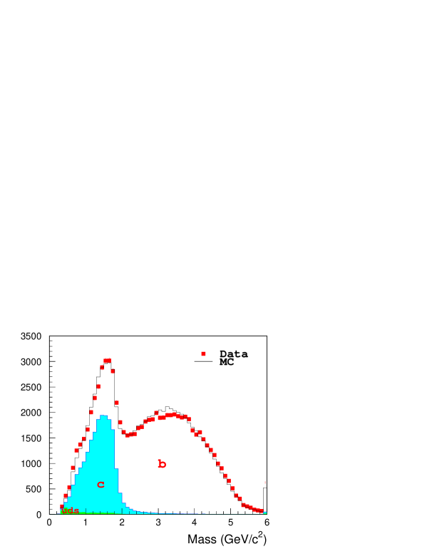
Figure 1: $p_{t}$ corrected vertex mass distribution for data (red square) and MC (solid line). White histogram is $b\overline{b}$ events, blue histogram is $c\overline{c}$ events, and green histogram is uds events [7].

3.2 $D_{s}^{-}$ $\rightarrow$ $\phi\pi^{-},K^{*0}K^{-}$ Reconstruction

$D_{s}^{-}$ candidates are reconstructed by first pairing oppositely charged tracks to form a $\phi$ ($K^{*0}$) candidate for the $\phi\pi^{-}$ ($K^{*0}K^{-}$) mode. A third track is then attached to form a $D_{s}$ candidate. Charged tracks used in the combination are required to have at least 23 CDC hits (out of possible 80 hits), at least 2 vertex detector hits, and a combined $\chi^{2}$/d.o.f. for the CDC+VXD3 fit of less than 8 to ensure good reconstruction. To maximize the discrimination between true $D_{s}$ and combinatorial background events, kinematic information for the $D_{s}$ candidate is fed into a neural net. The neural net inputs for the $\phi\pi$ ($K^{*0}K$) mode include: $K^{+}K^{-}$ ($K^{+}\pi^{-}$) invariant mass, fitted vertex probability of the $D_{s}$, total momentum of the $D_{s}$, helicity angle $\theta^{*}$ (angle between the $\phi$ ($K^{*0}$) and the $D_{s}$ flight directions in the $D_{s}$ rest frame), helicity angle $\lambda^{*}$ (angle between the charged daughter of the $D_{s}$ and the $K^{+}$ from $\phi$ ($K^{*0}$) decay in the rest frame of the neutral meson), and particle ID information for the three tracks. The complete list of neural net inputs is shown in Table 1.

$\phi\pi$  Mode	$K^{*0}K$  Mode
$D_{s}$ vertex $\chi^{2}$ prob	$D_{s}$ vertex $\chi^{2}$ prob
$P_{ptot}(D_{s})$	$P_{ptot}(D_{s})$
$KK$ opening angle	$K\pi$ (from $K^{*0}$) opening angle
$D_{s}$ normalized decay length	$D_{s}$ normalized decay length
helicity angle $\lambda^{*}$	helicity angle $\lambda^{*}$
helicity angle $\theta^{*}$	helicity angle $\theta^{*}$
particle ID of three tracks	particle ID of three tracks
	Average Normalized 3-D impact
	parameter of $KK\pi$ tracks

Table 1: $D_{s}$ Neural net inputs - left column is for $\phi\pi$ and right column is for $K^{*0}K$

The neural net is trained on Monte Carlo events generated using JETSET 7.4 [8] with full detector simulation based on GEANT 3.21 [9]. The neural net outputs are shown in Figure 2.

Figure 2: Neural Net outputs for (a) $\phi\pi$ and (b) $K^{*}K^{0}$ modes. Dots are data, open histograms are Monte Carlo and solid black histograms represent MC simulation of true Ds events.

The optimal neural net cut that maximizes the sensitivity of the analysis to $B_{s}^{0}$ mixing is determined separately for each of the two $D_{s}$ decay modes. The minimum cut for the $\phi\pi$ mode is determined to be at 0.9 and for the $K^{*0}K$ mode, is at 0.8. Furthermore, for the $K^{*0}K$ mode, the kaon from the $K^{*0}$ decay is required to be identified by the CRID in order to suppress combinatorial and other non-$D_{s}$ backgrounds. The $KK\pi$ invariant mass spectra are shown in Figures 3 and 4. The $D_{s}$ mass peak is fitted separately for events with and without definite kaon ID and for Q=0 and Q=$\pm$1 events, where Q is defined as the total charge of all tracks associated with the B decay. The details of the B vertex reconstruction and the $m_{KK\pi}$ mass fits are described in later sections.

Figure 3: Distribution of ${KK\pi}$ invariant mass for the $\phi\pi$ mode. Plots in the left column (a1,a2) are for the neutral candidates and plots in the right column (b1,b2) are for the charged candidates. The $\phi\pi$ sample is further subdivided into events with loose kaon ID (a1,b1) and events with hard kaon ID (a2,b2).

Figure 4: Distribution of ${KK\pi}$ invariant mass for the $K^{*}K^{0}$ mode. (a) for events with 1 kaon ID and (b) for events with 2 kaons ID.

The estimated number of $D_{s}$ candidates and combinatorial fractions are given in Table 2 and 3.

	Without Definite Kaon ID		With Definite Kaon ID
	Q=0	Q=$\pm$1	Q=0	Q=$\pm$1
# of hadronic candidates	101	57	54	40
# of semileptonic candidates	8	6	12	2
Average combinatorial fraction	42.3$\pm$2.1$\%$	53.8$\pm$2.7$\%$	21.7$\pm$2.2$\%$	14.1$\pm$1.4$\%$

Table 2: $\phi\pi$ mode– number of $D_{s}$ candidates within $\pm$ 40MeV of the nominal mass and the estimated average combinatorial fractions.

	1 Kaon ID	2 Kaons ID
	Q=0	Q=0
# of hadronic candidates	40	30
# of semileptonic candidates	6	5
Combinatorial fraction	32.9$\pm$3.3$\%$	22.3$\pm$2.2$\%$

Table 3: $K^{*0}K$ mode– number of $D_{s}$ candidates within $\pm$ 40MeV of the nominal mass and the estimated average combinatorial fractions.

4 B Proper Time and Vertex Charge Reconstruction

The $B_{s}^{0}$ oscillation frequency is expected to be large in the Standard Model and therefore a time dependent study of the phenomenon requires precision reconstruction of the $B_{s}^{0}$ proper decay time. The proper decay time is calculated from the reconstructed decay length ($\it{l}$) and the momentum of the $B_{s}^{0}$:

$$\tau_{B_{s}}=\frac{\it{l}}{\beta\gamma c},$$ (4)

where $\beta\gamma$, often referred to as “boost”, is the ratio between the momentum of the $B_{s}^{0}$ and its mass. In the following sections, the algorithms for reconstructing the decay length and the boost are described.

4.1 Decay Length Reconstruction

The decay length of the $B_{s}^{0}$ is defined as the distance between the IP and the $B_{s}^{0}$ decay vertex. The IP position is found by vertexing all tracks in the event to a common vertex. Taking advantage of the stability of the SLC beamspot, the IP position in the x-y plane (transverse to the beampipe) is averaged over 30 hadronic events. The position in z (beampipe direction) is calculated on an event-by-event basis. The estimated IP resolution for $Z^{0}\rightarrow b\,{\overline{b}}$ events is about 4$\mu m$ in x-y and 20$\mu m$ in z.

The $B_{s}^{0}$ decay vertex is found by vertexing the $D_{s}$ track with other $B$ decay tracks in the hemisphere. This is accomplished in two steps. The first step involves the selection of the seed vertex (preliminary estimate of the $B_{s}^{0}$ decay vertex). To find the seed, the $D_{s}$ track is individually vertexed with each quality track (excluding $D_{s}$ daughters) in the same hemisphere, and the vertex that is farthest from the IP and upstream (or consistent with being upstream within 5$\sigma$) of the $D_{s}$ and has a vertex fit $\chi^{2}$ of less than 5 is chosen as the seed. Step two involves the separation of tracks into secondary decay and fragmentation tracks. The discriminating variable used is the L/D parameter, where L is defined as the distance from the IP to the point of the closest approach of the candidate track to the seed vertex axis(line joining IP to the seed), and D is the distance from the IP to the seed. A track is chosen as a secondary B decay track if it satisfies the following two conditions: 1.) track L/D is greater than 0.5 and 2.) forms a good vertex with the $D_{s}$ track (fit $\chi^{2}\leq$ 5). The latter condition is imposed to reject spurious and B daughter tracks (from double charm decays) that do not point back to the B vertex. Finally, the selected tracks are then vertexed together with the $D_{s}$ to obtain the best estimate of the B decay position. The resulting B decay length resolution is highly dependent on the decay topology. The list of decay length resolutions estimated from Monte Carlo for the various decay categories is shown in Table 4.

	Q=0		Q=$\pm$1
Decay Category	Core $\sigma_{L}$($\mu m$)	Tail $\sigma_{L}$($\mu m$)	Core $\sigma_{L}$($\mu m$)	Tail $\sigma_{L}$($\mu m$)
$B_{s}^{0}\rightarrow D_{s}^{-}X$ (right-sign)	47	144	51	184
$B_{s}^{0}\rightarrow D_{s}^{+}X$ (wrong-sign)	89	292	89	292
$B_{d}^{0}\rightarrow D_{s}^{\pm}X$	70	271	85	412
$B_{u}\rightarrow D_{s}^{\pm}X$	99	435	72	236
$BBaryon\rightarrow D_{s}^{\pm}X$	84	221	84	221

Table 4: Decay length resolutions for various decay topologies. Resolutions are parameterized separately for neutral and charged B events except for wrong-sign $B_{s}^{0}$ and B Baryon events. The resolution is parameterized by the sum of two gaussians with core fraction fixed to 60$\%$.

4.2 Boost Reconstruction

To obtain the relativistic boost, the energy of the B meson has to be reconstructed. The total energy of the $B$ meson is the sum of the energy of the charged and neutral daughter particles:

$$E^{B}=E^{B}_{charged}+E^{B}_{neutral}.$$ (5)

The charged energy is determined by summing all the charged tracks associated with the B decay assuming pion mass (except for the two kaons from the $D_{s}$ decay). To estimate the neutral energy contribution, five different techniques are used. The first four techniques are calorimetery based and use various constraints (beam energy, jet energy, $B_{s}^{0}$ mass and calorimeter information) to estimate the neutral energy of the B meson [10]. The fifth technique is based only on the kinematics of the decay (B vertex axis, charged track momentum and $B_{s}^{0}$ mass constraint) to estimate the neutral energy [11]. The results from the five algorithms are then averaged, taking correlations into account, to obtain the total B energy. The relative boost resolutions $\sigma(\frac{\beta\gamma^{rec}-\beta\gamma^{true}}{\beta\gamma^{true}})$ are shown in Table 5.

	Q=0		Q=$\pm$1
Decay Category	Core $\sigma_{\beta\gamma}$($\%$)	Tail $\sigma_{\beta\gamma}$($\%$)	Core $\sigma_{\beta\gamma}$($\%$)	Tail $\sigma_{\beta\gamma}$($\%$)
$B_{s}^{0}\rightarrow D_{s}^{-}X$ (right-sign)	7.9	19.1	10.1	26.5
$B_{s}^{0}\rightarrow D_{s}^{+}X$ (wrong-sign)	8.6	19.7	11.1	28.3
$B_{d}^{0}\rightarrow D_{s}^{\pm}X$	9.5	19.6	9.1	24.7
$B_{u}\rightarrow D_{s}^{\pm}X$	10.4	30.0	8.4	21.1
$BBaryon\rightarrow D_{s}^{\pm}X$	10.0	25.4	11.1	39.6

Table 5: Relative boost resolutions for various decay topologies. The resolution is parameterized by the sum of two gaussians with core fraction fixed to 60$\%$.

4.3 Charge Reconstruction

Nominally, the charge of the $b$ hadron is the sum of the charge of the quality tracks associated with the B decay. To improve charge purity, tracks with only VXD3 hits (VX-alone vectors) that are not used in vertex and momentum reconstruction are also included in the B charge determination [6]. For the $\phi\pi$ mode, both the neutral B candidates (Q=0) and the charged candidates (Q=$\pm$1) are used. The $B_{s}^{0}$ purity in the charged sample is considerably lower than in the neutral sample and therefore has reduced weight in the fit. For the $K^{*0}K$ mode, only the neutral candidates are included in the final event sample. The reconstructed vertex charge distributions for data and Monte Carlo are shown in Figure 5.

Figure 5: Reconstructed B vertex charge distribution for data (dots), M.C. neutral B events (open histogram), and M.C. charged B events (solid histogram). The distribution is for the $\phi\pi$ and the $K^{*0}K$ modes combined.

5 Flavor Tagging

To decide whether mixing has occured for a given event, the flavor of the $B_{s}^{0}$ has to be determined at the production and the decay point. In this section, the methods used to tag the initial and final state of the $B_{s}^{0}$ are described.

5.1 Final State Flavor Tag

A significant fraction of the $B_{s}^{0}$ decays result in a $D_{s}$ in the final state. This knowledge is used not only to enhance the $B_{s}^{0}$ purity in the data sample but also as a means to determine the flavor of the $B_{s}^{0}$ at the decay vertex. For the final state tag, we assume the $D_{s}$ to come from the $b\rightarrow c$ transition which implies that a $\overline{B_{s}^{0}}$ would decay into a $D_{s}^{+}$ and a $B_{s}^{0}$ would decay into a $D_{s}^{-}$. However, roughly 10$\%$ of the time the virtual W produces a $D_{s}$ with an opposite sign. This process is the dominant source of final state mistag. The issue of final state mistag will be further addressed in a later section of this paper.

5.2 Initial State Flavor Tag

Several techniques are used to determine the initial state of the $B_{s}^{0}$. The most powerful method, unique to the SLD, is the polarization tag. In a polarized $Z^{0}\rightarrow b\overline{b}$ decay, the outgoing quark is produced preferentially along the direction opposite to the spin of the $Z^{0}$ boson. Therefore by knowing the helicity of the electron beam and the direction of the jet, the flavor of the primary quark in the jet can be inferred. The analyzing power of the polarization tag is highly dependent on the polar angle of the jet w.r.t. the beam axis and the electron beam polarization. The probability that the jet is a b quark jet is

$$P(b)=\frac{1+A_{FB}}{2},$$ (6)

where $A_{FB}$ is the polarized forward-backward asymmetry, defined as,

$$A_{FB}=2A_{b}\frac{A_{e}-P_{e}}{1-A_{e}P_{e}}\frac{cos\theta_{T}}{1+cos^{2}\theta_{T}},$$ (7)

with $A_{b}$ and $A_{e}$ assumed to have the Standard Model values of 0.935 and 0.150, respectively. The polar angle $\theta_{T}$ in equation (7) is defined as the angle between the thrust axis, which points in the event hemisphere, and the electron beam direction. $P_{e}$ is the electron beam polarization ($P_{e}>$ 0 for right handed and $<$ 0 for left handed electron beam).

In addition to the polarization tag, the momentum weighted jet charge technique is also used to determine the initial state of the $B_{s}^{0}$. The quantity $Q_{jet}$ is defined as the sum of the charge of the tracks in the opposite hemisphere weighted by the longitudinal momentum of the track w.r.t. the thrust axis, namely

$$Q_{jet}=\sum_{i}^{trks}{\left|\vec{p}_{i}\cdot\vec{T}\right|^{\kappa}},$$ (8)

where $\vec{T}$ is the thrust axis and $\kappa$ (equal to 0.5) is a parameter determined from Monte Carlo that maximizes the jet charge separation between $q$ and $\overline{q}$ jets. The probability of tagging the b quark hemisphere, given the opposite hemisphere jet charge $Q_{jet}$, is

$$P(b)=\frac{1}{1+e^{\alpha Q_{jet}}},$$ (9)

where the coefficient $\alpha$ is determined from Monte Carlo to be -0.27.

To further enhance the initial state tag purity, additional sources of information from the opposite hemisphere are used. This includes: vertex charge, charge of lepton, charge of kaon and dipole charge [12]. All the available tags in a given event are combined to obtain the overall initial state tag probability. For this analysis, the average initial state correct tag probability is about 75$\%$.

6 $B_{s}^{0}$ Oscillation Studies

The final step in a mixing analysis is to fit for the oscillation frequency. This entails a search for periodic oscillations in the proper decay time distribution of events tagged either as mixed or unmixed. We expect the proper time distribution, in the limit that the lifetime difference between the two mass eigenstates is small, to have the following time dependence for the mixed and unmixed events:

$$P_{mixed}(\tau)=\frac{e^{-\tau/\tau_{B_{s}}}}{2\tau}\left(1-cos(\Delta m_{s}\tau)\right),$$ (10)

$$P_{unmixed}(\tau)=\frac{e^{-\tau/\tau_{B_{s}}}}{2\tau}\left(1+cos(\Delta m_{s}\tau)\right).$$ (11)

Where $\tau_{B_{s}}$ is the $B_{s}^{0}$ lifetime and $\Delta m_{s}$ is the mass difference, as introduced in the earlier section. The fitting function used in the analysis also includes the effect of detector resolution, reconstruction efficiency, mistag, and background events. These details are addressed in the next few sections.

6.1 Amplitude Fit

The amplitude fit [13] is a fitting method that is used in this analysis. The method, in essence, transforms the traditional likelihood fit into a “Fourier-like” analysis. In an amplitude fit, the likelihood function is modified by introducing a term A, the amplitude, in front of the cosine terms ($\cos(\Delta m_{s}\tau)\rightarrow{\bf{A}}\cos(\Delta m_{s}\tau)$). Instead of fitting for $\Delta m_{s}$ directly, $\Delta m_{s}$ is fixed to a particular value and the parameter A is fitted for. The fit for A is repeated for a range of $\Delta m_{s}$ values to produce the amplitude plot. The amplitude is expected to be consistent with zero for values of $\Delta m_{s}$ far from $\Delta m_{s}^{true}$ and to reach unity at the true mass difference value. If the oscillation frequency is large and no signal is observed, the range of $\Delta m_{s}$ for which ${\bf A}+1.645\sigma_{A}\leq 1$ can be excluded at the 95$\%$ confidence level. The 95$\%$ C.L. sensitivity is defined as the value of $\Delta m_{s}$ at which $1.645\sigma_{A}=1$.

6.2 Likelihood Function

To perform the amplitude fit, we first need to construct a likelihood function that describes the proper time distribution of the events in the data sample. The events in the final sample can be divided into seven main sources, each with its own proper time distribution function, $F_{x}$. The seven physics sources are:

• $F_{B_{s}}^{r.s.}=B_{s}^{0}\rightarrow D_{s}^{-}X$ right sign decays + c.c.

• $F_{B_{s}}^{w.s.}=B_{s}^{0}\rightarrow D_{s}^{+}X$ wrong sign decays + c.c.

• $F_{B_{d}}=B_{d}^{0}\rightarrow D_{s}^{\pm}X$ + c.c.

• $F_{B^{\pm}}=B^{\pm}\rightarrow D_{s}^{\pm}X$ + c.c.

• $F_{BB}$ = B Baryon $\rightarrow D_{s}^{\pm}X$ + c.c.

• $F_{cc}$ = primary charm quark $\rightarrow D_{s}^{+}X$ + c.c.

• $F_{comb}$ = combinatorial events.

The proper time distribution of the event sample is the sum of the seven physics functions with the contribution from each source weighted by its fraction in the sample and the appropriate normalization constant. The resulting normalized probability distribution function for the mixed events is

$$P_{mixed}(\tau_{rec}) = {\it f_{D_{s}}(m_{KK\pi})}\left(\frac{{\it{f_{B_{s}}^{r.s.}}}}{N_{1}}F_{B_{s}}^{r.s.}+\frac{{\it{f_{B_{s}}^{w.s.}}}}{N_{2}}F_{B_{s}}^{w.s.}+\frac{{\it{f_{B_{d}}}}}{N_{3}}F_{B_{d}}+\frac{{\it{f_{B^{\pm}}}}}{N_{4}}F_{B^{\pm}}+\right.$$ (12)

$$\left.\frac{{\it{f_{BB}}}}{N_{5}}F_{BB}+\frac{{\it{f_{cc}}}}{N_{6}}F_{cc}\right)+\left[1-{\it f_{D_{s}}(m_{KK\pi})}\right]\cdot F_{comb}\ ,$$

where $\tau_{rec}$ is the reconstructed proper time, $\it{f_{D_{s}}}$ is the fraction of $D_{s}$ in the sample, $\it{f_{x}}$ is the fraction of category x in the $D_{s}$ signal peak, and $N_{i}$ is the normalization constant for category i. The physics functions for the mixed events have the following form:

$$F_{B_{s}}^{r.s.}(\tau_{rec}) = \int_{0}^{\infty}{\frac{e^{-\tau/\tau_{B_{s}}}}{2\tau_{B_{s}}}\left[(1-\eta_{i})\left(1-A\cdot cos(\Delta m_{s}\tau)\right)+\eta_{i}\left(1+A\cdot cos(\Delta m_{s}\tau)\right)\right]}\cdot$$ (13)

$$\epsilon_{1}(\tau)\cdot G_{1}(\tau,\tau_{rec})\ d\tau.$$

$$F_{B_{s}}^{w.s.}(\tau_{rec}) = \int_{0}^{\infty}{\frac{e^{-\tau/\tau_{B_{s}}}}{2\tau_{B_{s}}}\left[(1-\eta_{i})\left(1+A\cdot cos(\Delta m_{s}\tau)\right)+\eta_{i}\left(1-A\cdot cos(\Delta m_{s}\tau)\right)\right]}\cdot$$ (14)

$$\epsilon_{2}(\tau)\cdot G_{2}(\tau,\tau_{rec})\ d\tau.$$

$$F_{B_{d}}(\tau_{rec}) = \int_{0}^{\infty}{\frac{e^{-\tau/\tau_{B_{d}}}}{2\tau_{B_{d}}}\left[(1-\eta_{B_{d}})\left(1-cos(\Delta m_{d}\tau)\right)+\eta_{B_{d}}\left(1+cos(\Delta m_{d}\tau)\right)\right]}\cdot$$ (15)

$$\epsilon_{3}(\tau)\cdot G_{3}(\tau,\tau_{rec})\ d\tau.$$

$$F_{B^{\pm}}(\tau_{rec}) = \int_{0}^{\infty}{\frac{e^{-\tau/\tau_{B^{\pm}}}}{2\tau_{B^{\pm}}}\cdot\eta_{B^{\pm}}\cdot\epsilon_{4}(\tau)\cdot G_{4}(\tau,\tau_{rec})}\ d\tau.$$ (16)

$$F_{BB}(\tau_{rec}) = \int_{0}^{\infty}{\frac{e^{-\tau/\tau_{B_{BB}}}}{2\tau_{B_{BB}}}\cdot\eta_{BB}\cdot\epsilon_{5}(\tau)\cdot G_{5}(\tau,\tau_{rec})}\ d\tau.$$ (17)

$$F_{cc}(\tau_{rec}) = 5.47e^{-\tau_{rec}/0.2102}*erf(18.35\tau_{rec})\ \ \ (parameterized\ from\ M.C.).$$ (18)

$$F_{comb}(\tau_{rec}) = (distribution\ taken\ from\ data\ sidebands).$$ (19)

Where, $\tau$ is the true proper time, $\eta_{i}$ is the initial state mistag probability, $\eta_{B_{d,\pm,B}}$ are the overall mistag probabilities for $B_{d,\pm,B}$ events, and the last two functions: $\epsilon_{\it i}(\tau)$ and $G_{\it i}$($\tau,\tau_{rec}$) are the vertex efficiency and the resolution functions for category ${\it i}$, respectively. The proper time distribution for the combinatorial events is taken directly from the data using events in the sidebands. Detailed M.C. studies have shown that the combinatorial distribution is well modelled by the sidebands and that using the sideband distribution does not introduce a bias in the amplitude fit. The corresponding probability distribution for the unmixed events is obtained by replacing $\eta$ with ($1-\eta$) in the physics functions. Finally, the unbinned likelihood function is defined as the product of the probabilitiy of the mixed and unmixed events

$${\it{L}}=\prod_{i}^{mixed}P_{mxied}(\tau_{rec})\prod_{j}^{unmixed}P_{unmxied}(\tau_{rec}).$$ (20)

6.2.1 Data Compositions and Event Mistag Rate

The $D_{s}$ fraction ($\it{f_{D_{s}}}$) in equation (12) is the fraction of true $D_{s}$ events in the sample. Instead of using the average value from the mass plot, the $D_{s}$ fraction is determined on an event-by-event basis using the reconstructed $D_{s}$ mass of the candidate event. Events close to the nominal $D_{s}$ mass are more likely to be true $D_{s}$ events than combinatorial events, therefore have more significance in the analysis. The $D_{s}$ signal and background parameterizations used in the $\it{f_{D_{s}}}$ calculation are taken directly from the $m_{KK\pi}$ mass plot. The fitting function for the $D_{s}$ mass peak is the sum of two gaussians with the same mean and 60$\%$ core fraction. The widths used in the individual fits are fixed to the widths from the combined fit. The background is parameterized by a second order polynominal (combinatorial background) and a gaussian function$(D^{+}$ mass peak). For the $D^{+}$ gaussian, only the amplitude is allowed to float; the mean is fixed to 99.2MeV [14] below the fitted $D_{s}$ peak and the width is taken from the Monte Carlo distribution. The six dominant sources of $D_{s}$ production are outlined in the beginning of this section. The relative fractions of the sources are determined from the Monte Carlo and are estimated separately for the charged and neutral samples as well as for hadronic and semileptonic decays. The semileptonic decays are defined as events where a B decay track (not from the $D_{s}$ decay) is identified as either a muon or an electron. The relative fractions used in the fit are listed in Table 6 and 7.

	Hadronic Decays		Semileptonic Decays
	Q=0	Q=$\pm$1	Q=0	Q=$\pm$1
${\it f_{B_{s}}^{r.s.}}$	0.556	0.283	0.822	0.452
${\it f_{B_{s}}^{w.s.}}$	0.066	0.034	0.036	0.020
${\it f_{B_{d}}}$	0.260	0.160	0.122	0.129
${\it f_{B^{\pm}}}$	0.046	0.452	0.013	0.387
${\it f_{BB}}$	0.053	0.052	0.007	0.011
${\it f_{cc}}$	0.019	0.019	0.	0.

Table 6: Fractions for $\phi\pi$ mode.

	Hadronic Decays	Semileptonic Decays
	Q=0	Q=0
${\it f_{B_{s}}^{r.s.}}$	0.558	0.766
${\it f_{B_{s}}^{w.s.}}$	0.055	0.075
${\it f_{B_{d}}}$	0.252	0.117
${\it f_{B^{\pm}}}$	0.048	0.014
${\it f_{BB}}$	0.051	0.028
${\it f_{cc}}$	0.036	0.

Table 7: Fractions for $K^{*0}K$ mode.

The $B_{s}^{0}$ contribution to the likelihood function is divided into the right-sign and wrong-sign decay terms, and therefore, by construction, the final state mistag rate is 0 and 1, respectively, and does not enter explicitly into the likelihood. Instead, the effective final state mistag is accounted for in the relative $B_{s}^{0}$ right-sign and wrong-sign fraction. For the $B_{d}$ contribution, the right-sign and wrong-sign decays are not treated separately and the overall event mistag rate factors in both the inital state ($\eta_{i}$) and final state ($\eta_{f}^{B_{d}}$) mistags $\eta_{B_{d}}=\eta_{i}(1-\eta_{f}^{B_{d}})+\eta_{f}^{B_{d}}(1-\eta_{i})$. For $B^{\pm}$ and B Baryons, the overall event mistag rate is obtained by subsituting $\eta_{f}^{B_{d}}$ in the previous equation with $\eta_{f}^{B^{\pm}}$ and $\eta_{f}^{BB}$. The final state mistag rates are listed in Table 8 and the various measured branching ratios used in the calculation are listed in Table 10.

	$\eta_{f}$ (hadronic decay)	$\eta_{f}$ (semileptonic decays)
$B_{d}$	79.9$\%$	88.5$\%$
$B^{\pm}$	77.4$\%$	93.8$\%$
B Baryons	92.1$\%$	88.9$\%$

Table 8: Final state mistag rates for the hadronic and the semileptonic (events with a lepton attached to the B vertex) decays. For the $B_{d}$, $B^{\pm}$, and B baryon events, the $D_{s}$ primarily comes from the W decay, therefore, by definition, the final state mistag rates for those events are greater than 50$\%$.

6.2.2 Vertex Efficiency, Resolution Functions and Normalizations

To complete the discussion on the likelihood function, two remaining effects have to be addressed. First, the vertex efficiency function is included in the physics functions to account for the lower efficiency for reconstructing events with short proper time (events close to the IP). The efficiency functions are taken from the Monte Carlo simulations and are parameterized by the function:

$$\epsilon(\tau)=P_{1}\frac{1-e^{P_{2}\tau}}{1+e^{P_{2}\tau}}+P_{3}.$$ (21)

Equation (21) models the vertex efficiency well for the $B_{s}^{0}$, $B_{d}$ and B Baryons events. However, for the $B^{\pm}$, the vertex efficiency is also expected to decline at large proper times due to the B vertex charge requirement on the final sample(only candidates with Q=0,$\pm 1$ are kept). Therefore an additional exponential term ($P_{4}e^{-P_{5}\tau}$) is added to the function to model the behavior of the $B^{\pm}$ events. The coefficients ($P_{1-5}$) are listed in Table 9

Category	$P_{1}$	$P_{2}$	$P_{3}$	$P_{4}$	$P_{5}$
$\epsilon_{1},\epsilon_{2}$	0.148	-6.856	0.033
$\epsilon_{3}$	0.037	-4.448	0.032
$\epsilon_{4}$	0.061	-0.985	-1.209	1.243	0.007
$\epsilon_{5}$	0.056	-3.532	0.002

Table 9: Parameterizations for the vertex efficiency function.

The second effect concerns the proper time resolution. The effect is accounted for by introducing a resolution function in the convolution integrals, as shown in equations (13) to (17). The proper time resolution can be expressed in terms of the decay length and boost resolutions ($\sigma_{L}$,$\sigma_{\gamma\beta}$) as in

$$\sigma_{\tau}(\tau,i,j)=\left[\left(\frac{\sigma_{L}^{i}}{\gamma\beta c}\right)^{2}+\left(\tau\,\frac{\sigma_{\gamma\beta}^{j}}{\gamma\beta}\right)^{2}\right]^{1/2}\ ,$$ (22)

where the indices (i and j) refer to core or tail. The proper time resolution contains a constant term that depends on $\sigma_{L}$ and a term that rises linearly with proper time that depends on $\sigma_{\gamma\beta}$. This behavior is illustrated in Figure 6 for the $B_{s}^{0}$ events.

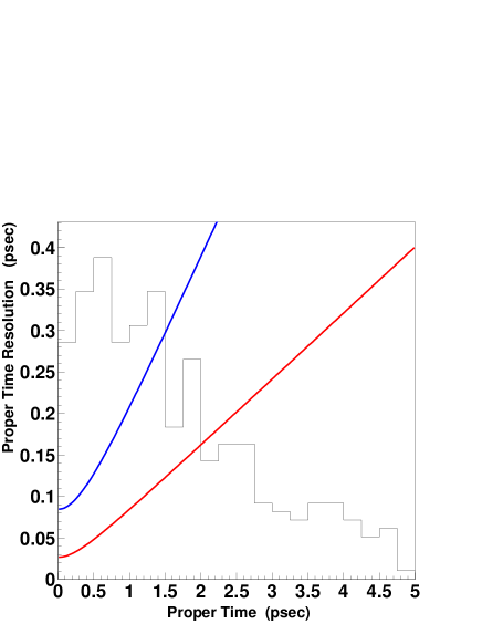
Figure 6: $\sigma_{\tau}$ distributions for $B_{s}^{0}\rightarrow D_{s}^{-}X$ events. The lower red line is calculated using $\sigma_{L}(core)$ and $\sigma_{\gamma\beta}(core)$. The upper blue line is calculated using $\sigma_{L}(tail)$ and $\sigma_{\gamma\beta}(tail)$. The background histogram is the proper time distribution of the data events.

In practice, there are four $\sigma_{\tau}$ distributions given by the various $\sigma_{L}$ and $\sigma_{\gamma\beta}$ core-tail combinations. The resolution function is obtained by summing all four contributions

$$G(\tau,\tau_{rec})={\it f^{2}_{c}}G_{cc}+{\it f_{c}}{\it f_{t}}(G_{ct}+G_{tc})+{\it f^{2}_{t}}G_{tt},$$ (23)

with ${\it f_{c}}$=0.6, ${\it f_{t}}$=0.4, and $G_{i,j}$ defined as

$$G_{i,j}=\frac{1}{\sqrt{2\pi}\sigma_{\tau}(\tau,i,j)}exp\left[{-(\tau-\tau_{rec})^{2}/2\sigma_{\tau}^{2}(\tau,i,j)}\right].$$ (24)

The complete likelihood function is normalized by dividing each physics term by a normalization constant. The normalization constant ($N_{\it i}$) is calculated for category ${\it i}$ by integrating the sum of the mixed and unmixed physics functions for source ${\it i}$ over all reconstructed proper times,

$$N_{\it i}=\int_{-\infty}^{+\infty}({F_{\it i}^{mixed}+F_{\it i}^{unmixed}})\ d{\tau_{rec}}.$$ (25)

The normalization is required to ensure that the weight of each physics source in the likelihood function is not biased by the efficiency and the proper time resolution of the event.

6.3 $D_{s}$+Tracks Amplitude Fit Results

The physics parameters used in the amplitude fit are listed in Table 10. The systematic uncertainties are calculated based on the formula [13]

$$\sigma_{A}^{syst}=A^{new}-A^{nominal}+(1-A^{nominal})\left(\frac{\sigma_{A}^{new}-\sigma_{A}^{nominal}}{\sigma_{A}^{nominal}}\right).$$ (26)

Parameter	Value and uncertainty	Reference
$\tau_{B_{s}}$	$1.464\pm 0.057\ ps$	[15]
$\tau_{B_{d}}$	$1.562\pm 0.029\ ps$	[15]
$\tau_{B^{\pm}}$	$1.656\pm 0.025\ ps$	[15]
$\tau_{BBaryons}$	$1.208\pm 0.051\ ps$	[15]
$\Delta m_{d}$	$0.476\pm 0.016\ ps^{-1}$	[15]
f($\overline{b}\rightarrow B_{s}^{0}$)	$0.1000\pm 0.012$	[15]
f($\overline{b}\rightarrow B_{d}^{0},B^{+}$)	$0.4010\pm 0.010$	[15]
f($\overline{b}\rightarrow B\ Baryon$)	$0.0990\pm 0.017$	[15]
$R_{b}\cdot{\cal B}(b\rightarrow\overline{B_{s}^{0}})\cdot{\cal B}(\overline{B_{s}^{0}}\rightarrow D_{s}^{+}X)\cdot{\cal B}(D_{s}^{+}\rightarrow\phi\pi^{+})$	$(6.21^{+0.73}_{-0.78})\times 10^{-4}$	[15, 16]
${\cal B}(b\rightarrow W^{-}\rightarrow D_{s}^{-})\cdot{\cal B}(D_{s}^{-}\rightarrow\phi\pi^{-})$	$(3.66\pm 0.45)\times 10^{-3}$	[16]
${\cal B}(B_{d,u}\rightarrow D_{s}^{\pm}X)\cdot{\cal B}(D_{s}^{-}\rightarrow\phi\pi^{-})$	$(3.71\pm 0.28)\times 10^{-3}$	[15]
${\cal B}(B_{d,u}\rightarrow D_{s}^{-}X)/{\cal B}(B_{d,u}\rightarrow D_{s}^{\pm}X)$	$0.172\pm 0.083$	[15]
${\cal B}(\overline{c}\rightarrow D_{s}^{-})\cdot{\cal B}(D_{s}^{-}\rightarrow\phi\pi^{-})$	$(3.4\pm 0.3)\times 10^{-3}$	[15]

Table 10: B lifetimes, $\Delta m_{d}$, B production fractions, and various branching ratios assumed in the amplitude fit. The uncertainties for the branching ratios do not include uncertainty from Br($D_{s}\rightarrow\phi\pi$). The right-sign $D_{s}$ production fraction ($R_{b}\cdot{\cal B}(b\rightarrow\overline{B_{s}^{0}})\cdot{\cal B}(\overline{B_{s}^{0}}\rightarrow D_{s}^{+}X)\cdot{\cal B}(D_{s}^{+}\rightarrow\phi\pi^{+})$) is obtained by combining the direct measurement [16] with the semileptonic measurement [15] assuming factorization.

The physics parameters are varied by $\pm 1\sigma$ in the fit to obtain the systematic uncertainties. In addition, the uncertainity on the $D_{s}$ signal fraction (${\it f}_{D_{s}}$) is estimated from the $D_{s}$ mass fit and is varied by roughly 8$\%$. The initial state tag probability is varied by $\pm 0.02$. The decay length resolution and the boost resolution uncertainties have not yet been studied in great detail and conservative estimates of 10$\%$ on $\sigma_{l}$ and 30$\%$ on $\sigma_{\gamma\beta}$ are used. A summary of the systematic uncertainties is given in Table 11

The resulting amplitude plot is shown in Figure 7.

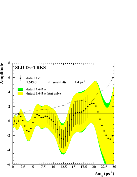
Figure 7: Ds+Tracks amplitude fit plot.

The measured values of the amplitudes are consistent with zero within the range of $\Delta m_{s}$ considered and no evidence of a signal is observed. This analysis excludes the following values of the $B_{s}^{0}-\overline{B_{s}^{0}}$ mixing oscillation frequency: $\Delta m_{s}<1.5$ ps^-1, $2.6<\Delta m_{s}<4.9$ ps^-1, and $10.8<\Delta m_{s}<13.5$ ps^-1 at the 95% confidence level (C.L.). The sensitivity at the 95% C.L. is 1.4 $ps^{-1}$. A comparison of the amplitudes and errors at $\Delta m_{s}$ = 15 $ps^{-1}$ for the various $B_{s}^{0}$ mixing analyses is shown in Figure 8 (this analysis is listed as “SLD Ds” in the figure).

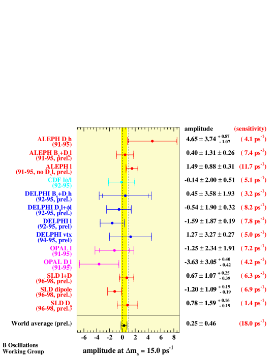
Figure 8: Amplitudes and errors at $\Delta m_{s}$=15$ps^{-1}$.

7 SLD Combination and Conclusion

The analysis presented in this paper is complementary to the two more inclusive analyses at the SLD: Charge Dipole and Lepton+D. Charge Dipole and Lepton+D have a combined sensitivity of 10 $ps^{-1}$ [12]. Figure 9 shows the amplitude fit for all three analyses combined. The combined plot takes into account the correlated systematic uncertainties. Furthermore, the samples were selected such as to remove any statistical overlap between analyses. No evidence of a signal is observed up to $\Delta m_{s}$ of 25 $ps^{-1}$ and the excluded regions at the 95% C.L. are: $\Delta m_{s}$ $<$ 7.6 $ps^{-1}$ and 11.8 $<$ $\Delta m_{s}$ $<$ 14.8 $ps^{-1}$. The SLD combined sensitivity at the 95% C.L. is 13.0 $ps^{-1}$.

$\Delta m_{s}$	5 ps-1	10 ps-1	15 ps-1	20 ps-1
Measured amplitude $A$	-0.260	-0.106	$0.781$	$-2.425$
Statistical uncertainty ($\sigma_{A}^{stat}$)	$\pm 0.813$	$\pm 1.058$	$\pm 1.591$	$\pm 1.817$
Total systematic uncertainty ($\sigma_{A}^{syst})$	${}^{+0.163}_{-0.136}$	${}^{+0.129}_{-0.098}$	${}^{+0.161}_{-0.193}$	${}^{+0.169}_{-0.221}$
$\tau_{B_{s}}$	${}^{+0.018}_{-0.019}$	${}^{+0.009}_{-0.009}$	${}^{+0.012}_{-0.013}$	${}^{+0.006}_{-0.007}$
$\tau_{B_{d}}$	${}^{-0.0006}_{+0.0006}$	${}^{-0.0005}_{+0.0005}$	${}^{-0.001}_{+0.001}$	${}^{-0.0002}_{-0.0002}$
$\tau_{B^{\pm}}$	${}^{-0.0007}_{+0.0007}$	${}^{-0.0002}_{+0.0002}$	${}^{+0.00002}_{-0.00002}$	${}^{-0.001}_{+0.001}$
$\tau_{B\ baryons}$	${}^{-0.00003}_{+0.00001}$	${}^{-0.00002}_{+0.00003}$	${}^{+0.0001}_{-0.0001}$	${}^{+0.002}_{-0.002}$
$\Delta m_{d}$	${}^{-0.0007}_{+0.0007}$	${}^{-0.0002}_{+0.0002}$	${}^{+0.00008}_{-0.00008}$	${}^{-0.00008}_{+0.00008}$
f($\overline{b}\rightarrow B_{s}^{0}$)	${}^{+0.020}_{-0.019}$	${}^{+0.010}_{-0.010}$	${}^{+0.003}_{-0.003}$	${}^{-0.0007}_{+0.0003}$
f($\overline{b}\rightarrow B\ Baryon$)	${}^{+0.007}_{-0.007}$	${}^{+0.002}_{-0.002}$	${}^{+0.002}_{-0.002}$	${}^{-0.005}_{+0.005}$
$\left(R_{b}\cdot{\cal B}(b\rightarrow\overline{B_{s}^{0}})\cdot\right.$	${}^{-0.048}_{+0.069}$	${}^{-0.017}_{+0.025}$	${}^{-0.0006}_{-0.0014}$	${}^{-0.0068}_{+0.0007}$
$\left.{\cal B}(\overline{B_{s}^{0}}\rightarrow D_{s}^{+}X)\cdot{\cal B}(D_{s}^{+}\rightarrow\phi\pi^{+})\right)$
${\cal B}(b\rightarrow W^{-}\rightarrow D_{s}^{-})\cdot{\cal B}(D_{s}^{-}\rightarrow\phi\pi^{-})$	${}^{+0.020}_{-0.020}$	${}^{+0.011}_{-0.010}$	${}^{+0.003}_{-0.003}$	${}^{-0.0008}_{+0.0003}$
${\cal B}(B_{d,u}\rightarrow D_{s}^{\pm}X)\cdot{\cal B}(D_{s}^{-}\rightarrow\phi\pi^{-})$	${}^{+0.021}_{-0.021}$	${}^{+0.006}_{-0.006}$	${}^{-0.0009}_{+0.0008}$	${}^{+0.008}_{-0.009}$
${\cal B}(B_{d,u}\rightarrow D_{s}^{-}X)/{\cal B}(B_{d,u}\rightarrow D_{s}^{\pm}X)$	${}^{+0.014}_{-0.013}$	${}^{+0.024}_{-0.024}$	${}^{+0.020}_{-0.021}$	${}^{+0.033}_{-0.040}$
${\cal B}(\overline{c}\rightarrow D_{s}^{-})\cdot{\cal B}(D_{s}^{-}\rightarrow\phi\pi^{-})$	${}^{+0.006}_{-0.006}$	${}^{+0.004}_{-0.004}$	${}^{-0.0004}_{+0.0003}$	${}^{-0.005}_{+0.005}$
Decay length resolution	${}^{+0.004}_{-0.003}$	${}^{+0.039}_{-0.038}$	${}^{+0.015}_{-0.019}$	${}^{+0.027}_{-0.040}$
Boost resolution	${}^{+0.052}_{-0.027}$	${}^{+0.075}_{-0.034}$	${}^{-0.166}_{+0.138}$	${}^{-0.147}_{+0.019}$
${\it f}_{D_{s}}$	${}^{+0.057}_{-0.055}$	${}^{+0.013}_{-0.011}$	${}^{+0.047}_{-0.051}$	${}^{+0.004}_{-0.006}$
Initial state tag	${}^{-0.102}_{+0.118}$	${}^{-0.075}_{+0.089}$	${}^{-0.079}_{+0.061}$	${}^{-0.155}_{+0.162}$

Table 11: Table of statistical and systematic uncertainties for several $\Delta m_{s}$ values.

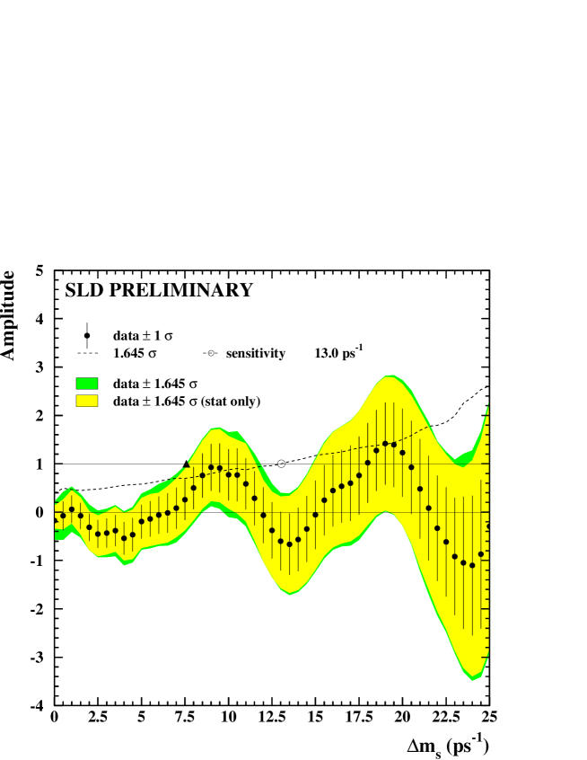
Figure 9: Combined SLD amplitude plot.

^∗∗ List of Authors

Kenji Abe,⁽¹⁵⁾ Koya Abe,⁽²⁴⁾ T. Abe,⁽²¹⁾ I. Adam,⁽²¹⁾ H. Akimoto,⁽²¹⁾ D. Aston,⁽²¹⁾ K.G. Baird,⁽¹¹⁾ C. Baltay,⁽³⁰⁾ H.R. Band,⁽²⁹⁾ T.L. Barklow,⁽²¹⁾ J.M. Bauer,⁽¹²⁾ G. Bellodi,⁽¹⁷⁾ R. Berger,⁽²¹⁾ G. Blaylock,⁽¹¹⁾ J.R. Bogart,⁽²¹⁾ G.R. Bower,⁽²¹⁾ J.E. Brau,⁽¹⁶⁾ M. Breidenbach,⁽²¹⁾ W.M. Bugg,⁽²³⁾ D. Burke,⁽²¹⁾ T.H. Burnett,⁽²⁸⁾ P.N. Burrows,⁽¹⁷⁾ A. Calcaterra,⁽⁸⁾ R. Cassell,⁽²¹⁾ A. Chou,⁽²¹⁾ H.O. Cohn,⁽²³⁾ J.A. Coller,⁽⁴⁾ M.R. Convery,⁽²¹⁾ V. Cook,⁽²⁸⁾ R.F. Cowan,⁽¹³⁾ G. Crawford,⁽²¹⁾ C.J.S. Damerell,⁽¹⁹⁾ M. Daoudi,⁽²¹⁾ S. Dasu,⁽²⁹⁾ N. de Groot,⁽²⁾ R. de Sangro,⁽⁸⁾ D.N. Dong,⁽²¹⁾ M. Doser,⁽²¹⁾ R. Dubois,⁽²¹⁾ I. Erofeeva,⁽¹⁴⁾ V. Eschenburg,⁽¹²⁾ S. Fahey,⁽⁵⁾ D. Falciai,⁽⁸⁾ J.P. Fernandez,⁽²⁶⁾ K. Flood,⁽¹¹⁾ R. Frey,⁽¹⁶⁾ E.L. Hart,⁽²³⁾ K. Hasuko,⁽²⁴⁾ S.S. Hertzbach,⁽¹¹⁾ M.E. Huffer,⁽²¹⁾ X. Huynh,⁽²¹⁾ M. Iwasaki,⁽¹⁶⁾ D.J. Jackson,⁽¹⁹⁾ P. Jacques,⁽²⁰⁾ J.A. Jaros,⁽²¹⁾ Z.Y. Jiang,⁽²¹⁾ A.S. Johnson,⁽²¹⁾ J.R. Johnson,⁽²⁹⁾ R. Kajikawa,⁽¹⁵⁾ M. Kalelkar,⁽²⁰⁾ H.J. Kang,⁽²⁰⁾ R.R. Kofler,⁽¹¹⁾ R.S. Kroeger,⁽¹²⁾ M. Langston,⁽¹⁶⁾ D.W.G. Leith,⁽²¹⁾ V. Lia,⁽¹³⁾ C. Lin,⁽¹¹⁾ G. Mancinelli,⁽²⁰⁾ S. Manly,⁽³⁰⁾ G. Mantovani,⁽¹⁸⁾ T.W. Markiewicz,⁽²¹⁾ T. Maruyama,⁽²¹⁾ A.K. McKemey,⁽³⁾ R. Messner,⁽²¹⁾ K.C. Moffeit,⁽²¹⁾ T.B. Moore,⁽³⁰⁾ M. Morii,⁽²¹⁾ D. Muller,⁽²¹⁾ V. Murzin,⁽¹⁴⁾ S. Narita,⁽²⁴⁾ U. Nauenberg,⁽⁵⁾ H. Neal,⁽³⁰⁾ G. Nesom,⁽¹⁷⁾ N. Oishi,⁽¹⁵⁾ D. Onoprienko,⁽²³⁾ L.S. Osborne,⁽¹³⁾ R.S. Panvini,⁽²⁷⁾ C.H. Park,⁽²²⁾ I. Peruzzi,⁽⁸⁾ M. Piccolo,⁽⁸⁾ L. Piemontese,⁽⁷⁾ R.J. Plano,⁽²⁰⁾ R. Prepost,⁽²⁹⁾ C.Y. Prescott,⁽²¹⁾ B.N. Ratcliff,⁽²¹⁾ J. Reidy,⁽¹²⁾ P.L. Reinertsen,⁽²⁶⁾ L.S. Rochester,⁽²¹⁾ P.C. Rowson,⁽²¹⁾ J.J. Russell,⁽²¹⁾ O.H. Saxton,⁽²¹⁾ T. Schalk,⁽²⁶⁾ B.A. Schumm,⁽²⁶⁾ J. Schwiening,⁽²¹⁾ V.V. Serbo,⁽²¹⁾ G. Shapiro,⁽¹⁰⁾ N.B. Sinev,⁽¹⁶⁾ J.A. Snyder,⁽³⁰⁾ H. Staengle,⁽⁶⁾ A. Stahl,⁽²¹⁾ P. Stamer,⁽²⁰⁾ H. Steiner,⁽¹⁰⁾ D. Su,⁽²¹⁾ F. Suekane,⁽²⁴⁾ A. Sugiyama,⁽¹⁵⁾ S. Suzuki,⁽¹⁵⁾ M. Swartz,⁽⁹⁾ F.E. Taylor,⁽¹³⁾ J. Thom,⁽²¹⁾ E. Torrence,⁽¹³⁾ T. Usher,⁽²¹⁾ J. Va’vra,⁽²¹⁾ R. Verdier,⁽¹³⁾ D.L. Wagner,⁽⁵⁾ A.P. Waite,⁽²¹⁾ S. Walston,⁽¹⁶⁾ A.W. Weidemann,⁽²³⁾ E.R. Weiss,⁽²⁸⁾ J.S. Whitaker,⁽⁴⁾ S.H. Williams,⁽²¹⁾ S. Willocq,⁽¹¹⁾ R.J. Wilson,⁽⁶⁾ W.J. Wisniewski,⁽²¹⁾ J.L. Wittlin,⁽¹¹⁾ M. Woods,⁽²¹⁾ T.R. Wright,⁽²⁹⁾ R.K. Yamamoto,⁽¹³⁾ J. Yashima,⁽²⁴⁾ S.J. Yellin,⁽²⁵⁾ C.C. Young,⁽²¹⁾ H. Yuta.⁽¹⁾

(The SLD Collaboration)

⁽¹⁾Aomori University, Aomori , 030 Japan, ⁽²⁾University of Bristol, Bristol, United Kingdom, ⁽³⁾Brunel University, Uxbridge, Middlesex, UB8 3PH United Kingdom, ⁽⁴⁾Boston University, Boston, Massachusetts 02215, ⁽⁵⁾University of Colorado, Boulder, Colorado 80309, ⁽⁶⁾Colorado State University, Ft. Collins, Colorado 80523, ⁽⁷⁾INFN Sezione di Ferrara and Universita di Ferrara, I-44100 Ferrara, Italy, ⁽⁸⁾INFN Lab. Nazionali di Frascati, I-00044 Frascati, Italy, ⁽⁹⁾Johns Hopkins University, Baltimore, Maryland 21218-2686, ⁽¹⁰⁾Lawrence Berkeley Laboratory, University of California, Berkeley, California 94720, ⁽¹¹⁾University of Massachusetts, Amherst, Massachusetts 01003, ⁽¹²⁾University of Mississippi, University, Mississippi 38677, ⁽¹³⁾Massachusetts Institute of Technology, Cambridge, Massachusetts 02139, ⁽¹⁴⁾Institute of Nuclear Physics, Moscow State University, 119899, Moscow Russia, ⁽¹⁵⁾Nagoya University, Chikusa-ku, Nagoya, 464 Japan, ⁽¹⁶⁾University of Oregon, Eugene, Oregon 97403, ⁽¹⁷⁾Oxford University, Oxford, OX1 3RH, United Kingdom, ⁽¹⁸⁾INFN Sezione di Perugia and Universita di Perugia, I-06100 Perugia, Italy, ⁽¹⁹⁾Rutherford Appleton Laboratory, Chilton, Didcot, Oxon OX11 0QX United Kingdom, ⁽²⁰⁾Rutgers University, Piscataway, New Jersey 08855, ⁽²¹⁾Stanford Linear Accelerator Center, Stanford University, Stanford, California 94309, ⁽²²⁾Soongsil University, Seoul, Korea 156-743, ⁽²³⁾University of Tennessee, Knoxville, Tennessee 37996, ⁽²⁴⁾Tohoku University, Sendai 980, Japan, ⁽²⁵⁾University of California at Santa Barbara, Santa Barbara, California 93106, ⁽²⁶⁾University of California at Santa Cruz, Santa Cruz, California 95064, ⁽²⁷⁾Vanderbilt University, Nashville,Tennessee 37235, ⁽²⁸⁾University of Washington, Seattle, Washington 98105, ⁽²⁹⁾University of Wisconsin, Madison,Wisconsin 53706, ⁽³⁰⁾Yale University, New Haven, Connecticut 06511.

References

- [1] See the following reviews: F. Caravaglios, F. Parodi, P. Roudeau, and A. Stocchi, Determination of the CKM unitarity triangle parameters by end 1999, hep-ph/0002171; S. Mele, Phys. Rev. D59, 113011 (1999).
- [2] S. Hashimoto, B decays on the lattice, hep-lat/9909136, Nucl. Phys. Proc. Suppl. 83, 3 (2000).
- [3] SLD Design Report, SLAC-R-273,UC-43D(1984), and revisions.
- [4] K. Abe et al., Nucl. Inst. and Meth. A400, 287 (1997).
- [5] D. J. Jackson, Nucl. Inst. and Meth. A388, 247 (1997).
- [6] K. Abe et al., Direct Measurement of using Charged Vertices, SLAC-PUB-8542, July 2000.
- [7] K. Abe et al., Improved Measurement of , at SLD, SLAC-PUB-8667, August 2000.
- [8] T. Sjöstrand, Comp. Phys. Comm. 82, 74 (1994).
- [9] R. Brun et al., Report No. CERN-DD/EE/84-1, 1989.
- [10] T. B. Moore, Ph.D. dissertation, Yale University, New Heaven, CT (1999).
- [11] D. Dong, Ph.D. dissertation, Massachusetts Institute of Technology, Cambridge, MA (1999); also SLAC-R-550.
- [12] K. Abe et al., Time Dependent Mixing Using Inclusive and Semileptonic Decays at SLD, SLAC-PUB-8568, August 2000.
- [13] H.-G. Moser and A. Roussarie, Nucl. Inst. and Meth. A384, 491 (1997).
- [14] Review of Particle Physics, Eur. Phys. J. C 15, 573 (2000).
- [15] ALEPH, CDF, DELPHI, L3, OPAL, and SLD Collaborations, Combined results on b-hadron production rates, lifetimes, oscillations, and semileptonic decays, SLAC-PUB-8492, June 2000.
- [16] ALEPH Collaboration, Measurement of meson production in decays and of the lifetime, Z. Phys. C 69 (1995) 585.