SLAC-PUB-8516 July 2000 Direct Measurement of $A_{b}$ at the $Z^{0}$ Pole Using a Lepton Tag

Abstract

We present a direct measurement of the parity violation parameter $A_{b}$, derived from the left-right forward-backward asymmetry of $b$ quarks tagged via leptons from semileptonic decays. The lepton identification algorithm combines information from tracking, calorimetry and from the SLD Cherenkov Ring Imaging Detector. The value of $A_{b}$ is extracted using a maximum likelihood fit to the differential cross section for fermion production. Vertexing information and decay kinematics have been used to discriminate among the different sources of tagged leptons. A new treatment of mixing effects and of background contamination has been introduced and a new vertexing algorithm has been used in the muon analysis. Based on the 1993-1998 SLD sample of 550K hadronic $Z^{0}$ decays with highly polarized electron beams, we have measured $A_{b}$ with a $\sim 3\%$ statistical error.

Submitted to the XXX International Conference on High Energy Physics
(ICHEP 2000), Osaka, Japan, Jul/27-Aug/2 2000.

1 Introduction

Parity violation in the $Zf\bar{f}$ coupling can be measured via the observables $A_{f}=2v_{f}a_{f}/(v^{2}_{f}+a^{2}_{f}),$ where $v_{f}$ and $a_{f}$ represent the vector and axial vector couplings to fermion $f$. The Born-level differential cross section for the reaction $e^{+}e^{-}\rightarrow Z^{0}\rightarrow f\bar{f}$ is

$${d\sigma_{f}}\,/\,{dz}\propto(1-A_{e}P_{e})(1+z^{2})+2A_{f}(A_{e}-P_{e})z\,,$$ (1)

where $P_{e}$ is the longitudinal polarization of the electron beam ($P_{e}>0$ for right-handed (R) polarization) and $z=\cos\theta$ is the direction of the outgoing fermion relative to the incident electron. In the presence of $e^{-}$ beam polarization, it is possible to construct the left-right forward-backward asymmetry

$${\tilde{A}}^{f}_{FB}(z)={{[\sigma_{L}^{f}(z)-\sigma_{L}^{f}(-z)]-[\sigma_{R}^{f}(z)-\sigma_{R}^{f}(-z)]}\over{[\sigma_{L}^{f}(z)+\sigma_{L}^{f}(-z)]+[\sigma_{R}^{f}(z)+\sigma_{R}^{f}(-z)]}}={{|P_{e}|A_{f}\,2z}\over{(1+z^{2})}}\,,$$ (2)

for which the dependence on the initial state coupling parameter $A_{e}$ disappears, allowing a direct measurement of the final state coupling parameters $A_{f}$. Thus electron beam polarization permits a unique measurement of $A_{f}$, independent of that inferred from the unpolarized forward-backward asymmetry[1] which measures the combination $A_{e}A_{f}$. In addition, the quantity $A_{b}$ is largely independent of propagator effects that modify the effective weak mixing angle, and so is complementary to other electroweak measurements performed at the $Z^{0}$ pole. In particular the Standard Model expectation $A_{b}~{}=~{}0.935$ has only a very slight dependence on the top quark and Higgs boson masses.
In this paper we present a direct measurement of $A_{b}$ based on identified leptons from semileptonic $B$ hadron decays. The analysis is based on the full 1993-1998 SLD data sample of 550,000 $Z^{0}$ decays and presents the improvements obtained with the addition of vertexing information provided by the new vertex detector (VXD3) installed in 1996. The measurement complements other direct measurements of $A_{b}$ performed at SLD, that use momentum-weighted track charge [4], vertex charge [5] and identified kaons [6] to determine the sign of the underlying quark in $b\bar{b}$ events. The lepton total and transverse momentum (with respect to the nearest jet), the mass of the event and some topological decay information are used to classify each event by deriving probabilities for the decays ($Z^{0}\rightarrow b\bar{b},b\rightarrow lepton$), ($Z^{0}\rightarrow b\bar{b},\bar{b}\rightarrow\bar{c}\rightarrow lepton$), ($Z^{0}\rightarrow b\bar{b},b\rightarrow\bar{c}\rightarrow lepton$), ($Z^{0}\rightarrow c\bar{c},\bar{c}\rightarrow lepton$), and ($Z^{0}\rightarrow background$) . The lepton charge ($Q$) provides quark-antiquark discrimination, while the jet nearest in direction to the lepton approximates the quark direction. The parameter $A_{b}$ is then extracted by a maximum likelihood fit of these data to the polarized differential cross section, taking into account the effects of hard gluon radiation. Although in this approach the polarized asymmetry (2) is not explicitly formed, the result for $A_{b}$ maintain its insensitivity to the initial state couplings.

2 Data Selection and Lepton Identification

The SLAC Linear Collider and its operation with a polarized electron beam have been described in detail elsewhere [9]. During the running period from 1993-98, the SLC Large Detector (SLD) recorded an integrated luminosity of 19.1 $pb^{-1}$ with a luminosity-weighted electron beam polarization of $|P_{e}|=0.729\pm 0.004$ (1997-98) at a mean center of mass energy of 91.27 GeV.

Charged particle tracks are reconstructed in the Central Drift Chamber [10] and the CCD-based vertex detector [11], in a uniform axial magnetic field of 0.6T. The combined momentum resolution in the plane perpendicular to the beam axis is $\delta p_{\bot}/p_{\bot}=\sqrt{(.01)^{2}+(.0026~{}p_{\bot}/GeV)^{2}\,}$.

The Liquid Argon Calorimeter (LAC) [12] measures the energies of charged and neutral particles and is also used for electron identification. The LAC is segmented into projective towers with separate electromagnetic and hadronic sections. In the barrel LAC, which covers the angular range $|\cos\theta|<0.82$, the electromagnetic towers have transverse size ${\rm\sim(36~{}mrad)^{2}}$ and are divided longitudinally into a front section of 6 radiation lengths and a back section of 15 radiation lengths. The barrel LAC electromagnetic energy resolution is ${{\sigma_{E}}/{E}}={{15\%}/{\sqrt{E(GeV)}}}$.

Muon tracking is provided by the Warm Iron Calorimeter (WIC) [13]. The WIC is 4 interaction lengths thick and surrounds the $2.8+0.7$ interaction lengths of the LAC and SLD magnet coil. Sixteen layers of plastic streamer tubes interleaved with 2 inch thick plates of iron absorber provide muon hit resolutions of 0.4 cm and 2.0 cm in the azimuthal and axial directions respectively.

The Cerenkov Ring Imaging Detector (CRID) [14] measures the velocities of charged tracks using the angles of Čerenkov photons emitted in liquid and gaseous radiators. Only the gas information has been included in this analysis, since the liquid covers only marginally the interesting momentum region ($p>2$ GeV/c). Electrons are distinguishable from pions in the region between 2 and 5 GeV and the muon identification (because of pion rejection) also improves considerably in this region. Kaon and proton rejection also helps the muon identification up to momenta of 15 GeV.

Hadronic events are selected by requiring at least 15 GeV of energy in the LAC and at least six tracks with $p_{\bot}>250~{}{\rm MeV}$. Approximately 550,000 events were found in the 1993-98 data sample, with negligible background. Jets are formed by combining calorimeter energy clusters according to the JADE algorithm [16] with parameter $y_{cut}=0.005$. The jet axis closely approximates the $b$-quark direction in $Z^{0}\rightarrow b\bar{b}$ events, with an angular resolution of ${\rm\sim 30~{}mrad}$. An electron or muon tag is used to select semi-leptonic decays. Electrons are identified with both LAC and CRID information for tracks with $p>2$ GeV in the angular range $|\cos\theta|<0.72$. Calorimeter information is used to build discriminant variables which exploit the characteristics of electromagnetic showers, including transverse and longitudinal shower development shapes, and matching of LAC energy and track momentum. The CRID information is stored in likelihood functions corresponding to each particle type hypothesis [15]. These quantities are used as input variables to a Neural Network, trained on Monte Carlo tracks [17]. The effficiency (purity) for electron identification is on average 62$\%$ (70$\%$) and over 78$\%$ (80$\%$) for electrons with momenta greater than 15 GeV/c. This estimate includes electrons from photon conversions as signal. As pion misidentification is the largest contribution to the background, the simulation has been verified using charged pions from reconstructed $K^{0}_{s}\rightarrow\pi^{+}\pi^{-}$ decays. The fraction of such pions misidentified as electrons is $(1.23\pm 0.15)\%$, consistent with a MC expectation of $(1.36\pm 0.07)\%$. Electrons from photon conversions are removed from the sample with a 70$\%$ efficiency. The remaining photon conversion background is clustered at low momentum, away from most of the signal region.

Muon identification is performed for tracks with $p>2$ GeV in the angular range $|\cos\theta|<0.70$, although the muon identificaton efficiency falls off rapidly for $|\cos\theta|>0.60$ (in the region between the barrel and the endcaps). CDC tracks are extrapolated along with the associated error matrices, including multiple scattering, and matched with hit patterns in the WIC. For $|\cos\theta|<0.60$, 87$\%$ of the simulated muon tracks have successful matching between the CDC and the WIC. The second step of the muon identification exploits the information from the CRID. The CRID $k-\mu$ separation variable alone rejects $51\%$ of the remaining $k$ and $p$ (with only $2\%$ loss in the signal), while, for $p<6$ GeV, the $\pi-\mu$ separation variable rejects $37\%$ of $\pi$ (with $5\%$ loss in the signal). Since the CRID information is intrinsically momentum dependent, different sets of cuts on the distributions of the discriminant variables have been optimized in different momentum regions to achieve best purity and efficiency. The purity of the final sample is improved by requiring that the candidate muons fully penetrate the WIC, and by applying further cuts on the number of hits associated with the tracks, on the $\chi^{2}$ of the CDC/WIC matching and on the $\chi^{2}$ of the fit of the track in the WIC. MC studies show that pion punch through background is negligible. Muons from pion and kaon decays and hadronic showers are a significant background, but fall off rapidly with increasing momentum. From a study on a pure pions data sample, obtained from kinematically selected $K^{0}_{s}\rightarrow\pi^{+}\pi^{-}$ decays, $\sim.3\%$ of pions, with $p>2$ GeV, are identified as muons. The muon identification efficiency is over $81\%$ with a purity of $68\%$ ($8\%$ misidentified tracks and $24\%$ muons from light hadron decays) for $p>2$ GeV and $|\cos\theta|<0.60$.

3 Monte Carlo Simulation

The likelihood that an identified lepton comes from each of the physics sources ($b\rightarrow{l}$, $b\rightarrow{c}\rightarrow{l}$, $c\rightarrow{l}$, background etc.) relies directly on MC simulation. $Z^{0}$ decays are generated by the JETSET 7.4 program [18]. The $B$ hadron decay model was tuned to reproduce existing data from other experiments. Semileptonic decays of $B$ mesons are generated according to the ISGW formalism [19] with a 23$\%$ $D^{**}$ fraction, while semileptonic decays of $D$ mesons are generated with JETSET with the 1994 Particle Data Group branching ratios [20]. Particularly important experimental constraints are provided by the $B\rightarrow lepton$ and $B\rightarrow D$ momentum spectra measured by CLEO [21] [22], the $D\rightarrow lepton$ momentum spectrum measured by DELCO [23], and the $B\rightarrow hadron$ multiplicities measured by ARGUS [24].

The SLD detector response is simulated in detail using GEANT [25] and has been checked extensively against $Z^{0}$ data.

4 Vertex Mass Reconstruction

Vertex identification is done topologically, by searching for space points in 3D where track density functions overlap [3]. Each track is parametrized by a Gaussian probability density tube with a width equal to the uncertainty in the measured track position at the IP. Points that are characterized by a large overlap of these Gaussian probability tubes are considered candidate (seed) vertices. By clustering maxima in the density distribution, secondary vertices are found for the two hemispheres. The efficiency for reconstructing a vertex in the same hemisphere as the lepton is $\sim 66\%$ (1996-98). The mass of the secondary vertex is calculated using the tracks attached to the vertex itself. Each track is assigned the mass of a charged pion and the invariant mass of the vertex is thus calculated. This is then corrected to account for neutral particles by using kinematic information. By comparing the vertex flight path and the momentum sum of the tracks associated to the secondary vertex, one calculates a minimum amount of missing transverse momentum to be added to the invariant (raw) mass. This is done by assuming that the true quark momentum is aligned with the flight direction of the vertex. The so-called $P_{t}$-corrected mass is then given by:

$$M_{VTX}=\sqrt{M_{raw}^{2}+P_{t}^{2}}+|P_{t}|$$ (3)

We require that the transverse momentum contribution be less than the initial mass of the secondary vertex, to ensure that poorly measured vertices in $uds$ events do not leak into the final sample by adding large $P_{t}$.

5 Maximum Likelihood Fit

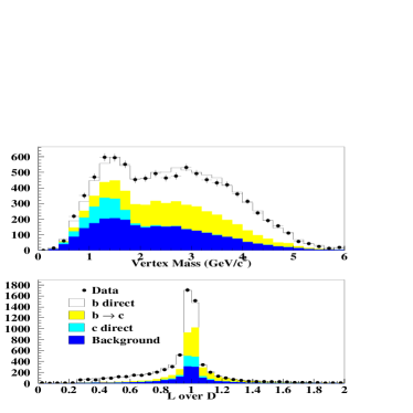
Figure 7: Vertex mass and L/D distributions for electrons in the data (dots) and Monte Carlo (histogram).

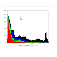
Figure 11: Electron NN output, background output.

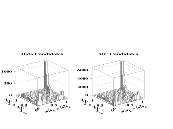
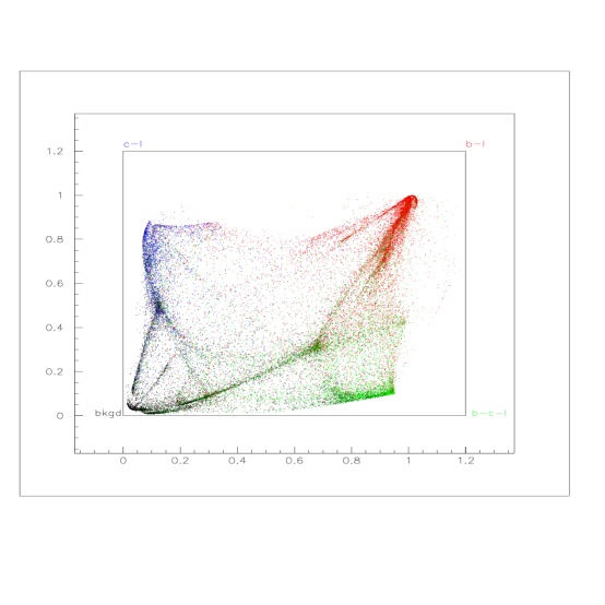
Figure 12: Dalitz space plot of Neural Network output for data and Monte Carlo candidates.

Figure 13: Dalitz space plot for Monte Carlo candidates. Ideally, $b$ direct decays should be clustered around (1,1), $b$ cascade decays at (0,1), charm decays at (0,1) and background events at (0,0).

Separation between the various lepton sources is accomplished using kinematic and vertexing information. Probabilities for each of the decay processes are assigned to every lepton, and calculated separately for electrons and muons.
For electron candidates, eight discriminating variables are calculated based on characteristics of the event [7]. These are track momentum ($p$), momentum transverse to the nearest jet ($p_{t}$), same hemisphere vertex mass, same hemisphere vertex momentum, same hemisphere vertex significance, ratio of the track longitudinal distance from the IP along the vertex axis to the vertex distance from the IP (L/D, see fig. 1), estimate of the underlying $b$ quark boost, and the opposite hemisphere vertex mass (fig. 7). (Note: vertexing variables are not always all available for every event, but there is a requirement on the presence of a reconstructed vertex in at least one hemisphere.) These variables are fed into an Artificial Neural Network, configured with 1 input layer, 2 hidden layers, and 4 output nodes (see figs. 11, 11, 11, 11). The Neural Network weights are set by training on a Monte Carlo simulation of semileptonic decays of heavy quarks in $Z^{0}$ decays. The output of the Neural Network is checked with data. The probabilities are assigned by transforming the 3 NN output nodes onto a 2 dimensional space by $x=NN_{b}+NN_{bc}$ and $y=NN_{b}+NN_{c}$, illustrated graphically by figs. 13 and  13. This space is divided up into bins and every candidate is assigned classification probabilites based on the number of events of each type in its corresponding bin.

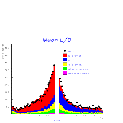
Figure 5: L/D distribution for muons in 1996-98 data (dots) and Monte Carlo (histogram).

For the muon candidates, a multi-variate analysis is applied [8]. Decay probabilities are calculated for every muon in the data by using a nearest neighbours technique in a 3-D Monte Carlo phase space. Three planes are defined, corresponding to three different ranges of the event mass (defined as the largest of the masses reconstructed in the two opposite hemispheres of the event, fig. 5): $\geq$ 2 GeV, $2>M_{vtx}\geq 0.55$ and $0.55>M_{vtx}\geq 0$ (or no vertex found) . These planes are parametrized by the quantities $\sqrt{P_{t}}$ and $\ln|P|/2$, to ensure a more uniform point distribution (also the scales for the two variables are roughly the same, see fig. 6). The weights for a muon in the data are then calculated with a nearest neighbours technique, by selecting all MC events within a fixed distance  from the data point in the corresponding plane and deriving the fractions of events of each type in this sample. In a second step and for those events only with a reconstructed vertex mass, these probabilities are re-weighted with fractions derived from the MC L/D distribution (see fig. 5), which account for the likelihood of an event coming from a certain source to have a value of L/D included in a specific interval. This information helps particularly to enhance the ability in separating $b$ direct decays from $b$ cascade decays (which have the “wrong” charge association). Correlations between all the different physical quantities employed have been taken into account. A cross-check via a neural network approach (similar to the one used for the electrons) has been performed and it has given consistent results.

A maximum likelihood analysis of all hadronic $Z^{0}$ events containing leptons is used to determine $A_{b}$. The likelihood function contains the following probability term for each lepton in the data:

$$P\,(p,p_{t},mass,L/D\,P_{e},z;\,A_{b},A_{c}) \propto=\left\{(1+z^{2})(1-A_{e}P_{e})-2Q(A_{e}-P^{i})\right.$$ (4)

$$\left[(f_{b}-f_{bc}+f_{b\bar{c}})(1-2\chi_{i})(1-\Delta^{b}_{QCD}(z))A_{b}\right.$$

$$\left.\left.+f_{c}(1-\Delta^{c}_{QCD}(z))A_{c}+f_{bkg}A_{bkg}\right]z\right\}.$$

where $z=\cos\theta_{jet}$. The three signs governing the left-right forward-backward asymmetry — beam polarization $P_{e}$, lepton charge $Q$, and jet direction $\cos\theta$ — are incorporated automatically into the maximum likelihood probability function. The fractions ($f_{b},f_{bc},f_{b\bar{c}},f_{c},f_{bkg}$) are the lepton decay probabilities for the different decay modes, derived from the MC simulation as described before. A correction factor $(1-2\chi_{i})$ is applied to all b-quark lepton sources to account for asymmetry dilution due to $B^{0}\bar{B}^{0}$ mixing. For the electrons an average $\bar{\chi}=0.1260$ is calculated from Monte Carlo (to account for the analysis bias introduced by the vertex requirement), and rescaled for $b$ cascade events to account for different mixing probabilities ($\bar{\chi}=0.1364$ and $\bar{\chi}=0.1376$ are used for $b\rightarrow{c}\rightarrow{e}$ and $b\rightarrow{\bar{c}}\rightarrow{e}$ events respectively). For the muon analysis, $\chi$ is calculated event by event using the truth mixing information of MC events closest to the data point in a phase space parametrized by $(p,p_{t},mass,L/D)$. The dependency on the event lifetime is thus automatically accounted for without any further need of rescaling. The background asymmetry $A_{bkg}$ is derived for the electron analysis as a function of $p$ and $p_{t}$ from tracks in the data not identified as leptons. For muons instead, it is calculated as a function of $p$ and $p_{t}$ (using the same procedure) from MC true background muons, divided in two samples: misidentified muons and light hadron muons (or misassociated tracks). A $cos\theta$ dependent QCD correction factor is applied to the theoretical asymmetry function to incorporate known QCD corrections to the cross section. The quantity $\Delta^{f}_{QCD}(z)$ has been calculated at $O(\alpha_{s})$ for massive final state quarks by Stav and Olsen [26] and is as large as 5$\%$ for the b quark at $z\!=\!0$. For an unbiased sample of $b\bar{b}$ events with $|z|<0.7$, correcting for this effect increases the asymmetry by $3\%$ overall. However, the theoretical calculations assume perfect efficiency in the reconstruction of events with emission of gluons of any energy. The inefficiency of the detector and the presence of cuts and weights in the analysis cause biases in the event selection which favor $q\bar{q}$ events over $q\bar{q}g$ events, therefore the QCD correction to be applied is less than the theoretical one. The effects of this and other related biases have been studied with a MC simulation of the analysis chain and corrected for in the likelihood function as a function of $\theta$, decreasing the theoretical QCD correction by about 30$\%$ [27]. $O(\alpha_{s}^{2})$ QCD effects are mainly due to two contributions: gluon splitting and second order hard gluon radiation. The gluon splitting correction is calculated apart by re-fitting for $A_{b}$ (in a MC as data study) after having excluded from the MC all the $g\rightarrow{b\bar{b}}$, $g\rightarrow{c\bar{c}}$ events. The difference in the central values, rescaled by the ratio of the current world measurements (OPAL) [1] of the gluon splitting fractions to the JETSET input values, is assumed as correction. For the second order gluon radiation effects, recent theoretical calculations by Ravindran and van Neerven [28] have been implemented. These have been worked out for different values of the quark masses (pole masses or running) and they predict effects about four times as big as in previous calculations ($\sim 1\%$ correction on $A_{b}$).

6 Results and Systematic Errors

The results obtained for the 1993-98 data are as follows, where the combined result takes into account the systematic correlations between the muon and electron analyses.

$$Muons A_{b}=0.950~{}\pm~{}0.038_{\it stat}~{}\pm~{}0.026_{\it syst}$$ (5)

$$Electrons A_{b}=0.876~{}\pm~{}0.045_{\it stat}~{}\pm~{}0.028_{\it syst}$$

$$Combined A_{b}=0.922~{}\pm~{}0.029_{\it stat}~{}\pm~{}0.024_{\it syst}$$

A list of systematic errors is shown in Table 1. The background levels have been studied with the MC, but also with a data sample of pure pions from $K^{0}_{s}$ decays. The asymmetry of the background has been varied by $\pm 40\%$ of itself for the electron analysis, and just rescaled by the ratio of the asymmetry in data and MC for charged non-leptonic tracks in the muon case. Uncertainty in the jet axis simulation can affect the asymmetry measurement by distorting the lepton $p_{t}$ spectrum and, to a lesser extent, the jet direction. The resulting systematic error has been studied by comparing the back-to-back direction of jets for data and MC in two jet events. The electron sample is more sensitive to such effects since both jet finding and electron identification algorithm rely on the same calorimeter response. The precision of the $B^{\pm}$ and $B^{0}$ lepton spectra is directly related to the uncertainty in the $D^{**}$ branching fraction reported by the CLEO collaboration [21]. The systematic error due to uncertainties in the D lepton spectrum has been estimated by constraining the ACCMM model [2] to the DELCO $D\rightarrow l$ data [23]. The systematic error due to the QCD correction includes uncertainties in the 2nd order QCD calculations for hard gluon emission and gluon splitting, in the value of $\alpha_{s}$, and in the bias due to event selection criteria in the analysis. This analysis is independent of tracking efficiency, unless such efficiency depends on $p$, $p_{t}$ or is not symmetric in $\cos\theta$. The extent of this $p$ and $p_{t}$ dependence has been constrained by reweighting MC tracks by the ratio of the number of tracks in data and MC as a function of $p$ and $p_{t}$. The extracted value of $A_{f}$ is much less sensitive to potential differences in the relative efficiency for selecting leptons between the forward and backward hemispheres than are the values of $A_{f}$ extracted from the unpolarized forward-backward asymmetry. The relative suppression factor is greater than $1/{A_{e}}^{2}\sim 50$ for any value of $|z|$ and therefore forward-backward asymmetry in the detector acceptance is not a significant source of measurement bias. $A_{c}$ has been fixed in the maximum likelihood fit to its Standard Model value, and a systematic error has been calculated by varying this number by plus or minus twice the current statistical uncertainty on the world average of the $A_{c}$ measurements.

The value obtained for $A_{b}$ from leptons can be combined with the other measurements performed at the SLC/SLD, respectively based on a momentum weighted track charge method, a vertex charge method and kaon decays. The resulting SLD average

$A_{b}=0.914~{}\pm~{}0.024,$

obtained using the data collected in 1993-1998, is consistent with the SM prediction $A_{b}=0.935$ and in agreement with recent preliminary results from LEP and SLD[1].

7 Conclusions

In conclusion, we have measured the extent of parity violation in the coupling of $Z^{0}$ bosons to $b$ quarks by using identified charged leptons from semileptonic decays. The analysis presented in this paper is based on the entire sample of 550,000 $Z^{0}$ decays collected in 1993-98 at SLD and employs vertexing information to separate the different decay sources. The resulting 1993-98 measurement

$A_{b}=0.922~{}\pm~{}0.029~{}\pm~{}0.024,$

represents an improvement relative to previous measurements[30].

8 Acknowledgements

We thank the staff of the SLAC accelerator department for their outstanding efforts on our behalf. This work was supported by the U.S. Department of Energy and National Science Foundation, the UK Particle Physics and Astronomy Research Council, the Istituto Nazionale di Fisica Nucleare of Italy and the Japan-US Cooperative Research Project on High Energy Physics.

^∗ List of Authors

Koya Abe,⁽²⁴⁾ Kenji Abe,⁽¹⁵⁾ T. Abe,⁽²¹⁾ I. Adam,⁽²¹⁾ H. Akimoto,⁽²¹⁾ D. Aston,⁽²¹⁾ K.G. Baird,⁽¹¹⁾ C. Baltay,⁽³⁰⁾ H.R. Band,⁽²⁹⁾ T.L. Barklow,⁽²¹⁾ J.M. Bauer,⁽¹²⁾ G. Bellodi,⁽¹⁷⁾ R. Berger,⁽²¹⁾ G. Blaylock,⁽¹¹⁾ J.R. Bogart,⁽²¹⁾ G.R. Bower,⁽²¹⁾ J.E. Brau,⁽¹⁶⁾ M. Breidenbach,⁽²¹⁾ W.M. Bugg,⁽²³⁾ D. Burke,⁽²¹⁾ T.H. Burnett,⁽²⁸⁾ P.N. Burrows,⁽¹⁷⁾ A. Calcaterra,⁽⁸⁾ R. Cassell,⁽²¹⁾ A. Chou,⁽²¹⁾ H.O. Cohn,⁽²³⁾ J.A. Coller,⁽⁴⁾ M.R. Convery,⁽²¹⁾ V. Cook,⁽²⁸⁾ R.F. Cowan,⁽¹³⁾ G. Crawford,⁽²¹⁾ C.J.S. Damerell,⁽¹⁹⁾ M. Daoudi,⁽²¹⁾ S. Dasu,⁽²⁹⁾ N. de Groot,⁽²⁾ R. de Sangro,⁽⁸⁾ D.N. Dong,⁽¹³⁾ M. Doser,⁽²¹⁾ R. Dubois, I. Erofeeva,⁽¹⁴⁾ V. Eschenburg,⁽¹²⁾ E. Etzion,⁽²⁹⁾ S. Fahey,⁽⁵⁾ D. Falciai,⁽⁸⁾ J.P. Fernandez,⁽²⁶⁾ K. Flood,⁽¹¹⁾ R. Frey,⁽¹⁶⁾ E.L. Hart,⁽²³⁾ K. Hasuko,⁽²⁴⁾ S.S. Hertzbach,⁽¹¹⁾ M.E. Huffer,⁽²¹⁾ X. Huynh,⁽²¹⁾ M. Iwasaki,⁽¹⁶⁾ D.J. Jackson,⁽¹⁹⁾ P. Jacques,⁽²⁰⁾ J.A. Jaros,⁽²¹⁾ Z.Y. Jiang,⁽²¹⁾ A.S. Johnson,⁽²¹⁾ J.R. Johnson,⁽²⁹⁾ R. Kajikawa,⁽¹⁵⁾ M. Kalelkar,⁽²⁰⁾ H.J. Kang,⁽²⁰⁾ R.R. Kofler,⁽¹¹⁾ R.S. Kroeger,⁽¹²⁾ M. Langston,⁽¹⁶⁾ D.W.G. Leith,⁽²¹⁾ V. Lia,⁽¹³⁾ C. Lin,⁽¹¹⁾ G. Mancinelli,⁽²⁰⁾ S. Manly,⁽³⁰⁾ G. Mantovani,⁽¹⁸⁾ T.W. Markiewicz,⁽²¹⁾ T. Maruyama,⁽²¹⁾ A.K. McKemey,⁽³⁾ R. Messner,⁽²¹⁾ K.C. Moffeit,⁽²¹⁾ T.B. Moore,⁽³⁰⁾ M. Morii,⁽²¹⁾ D. Muller,⁽²¹⁾ V. Murzin,⁽¹⁴⁾ S. Narita,⁽²⁴⁾ U. Nauenberg,⁽⁵⁾ H. Neal,⁽³⁰⁾ G. Nesom,⁽¹⁷⁾ N. Oishi,⁽¹⁵⁾ D. Onoprienko,⁽²³⁾ L.S. Osborne,⁽¹³⁾ R.S. Panvini,⁽²⁷⁾ C.H. Park,⁽²²⁾ I. Peruzzi,⁽⁸⁾ M. Piccolo,⁽⁸⁾ L. Piemontese,⁽⁷⁾ R.J. Plano,⁽²⁰⁾ R. Prepost,⁽²⁹⁾ C.Y. Prescott,⁽²¹⁾ B.N. Ratcliff,⁽²¹⁾ J. Reidy,⁽¹²⁾ P.L. Reinertsen,⁽²⁶⁾ L.S. Rochester,⁽²¹⁾ P.C. Rowson,⁽²¹⁾ J.J. Russell,⁽²¹⁾ O.H. Saxton,⁽²¹⁾ T. Schalk,⁽²⁶⁾ B.A. Schumm,⁽²⁶⁾ J. Schwiening,⁽²¹⁾ V.V. Serbo,⁽²¹⁾ G. Shapiro,⁽¹⁰⁾ N.B. Sinev,⁽¹⁶⁾ J.A. Snyder,⁽³⁰⁾ H. Staengle,⁽⁶⁾ A. Stahl,⁽²¹⁾ P. Stamer,⁽²⁰⁾ H. Steiner,⁽¹⁰⁾ D. Su,⁽²¹⁾ F. Suekane,⁽²⁴⁾ A. Sugiyama,⁽¹⁵⁾ A. Suzuki,⁽¹⁵⁾ M. Swartz,⁽⁹⁾ F.E. Taylor,⁽¹³⁾ J. Thom,⁽²¹⁾ E. Torrence,⁽¹³⁾ T. Usher,⁽²¹⁾ J. Va’vra,⁽²¹⁾ R. Verdier,⁽¹³⁾ D.L. Wagner,⁽⁵⁾ A.P. Waite,⁽²¹⁾ S. Walston,⁽¹⁶⁾ A.W. Weidemann,⁽²³⁾ E.R. Weiss,⁽²⁸⁾ J.S. Whitaker,⁽⁴⁾ S.H. Williams,⁽²¹⁾ S. Willocq,⁽¹¹⁾ R.J. Wilson,⁽⁶⁾ W.J. Wisniewski,⁽²¹⁾ J.L. Wittlin,⁽¹¹⁾ M. Woods,⁽²¹⁾ T.R. Wright,⁽²⁹⁾ R.K. Yamamoto,⁽¹³⁾ J. Yashima,⁽²⁴⁾ S.J. Yellin,⁽²⁵⁾ C.C. Young,⁽²¹⁾ H. Yuta.⁽¹⁾

⁽¹⁾Aomori University, Aomori, 030 Japan, ⁽²⁾University of Bristol, Bristol, United Kingdom, ⁽³⁾Brunel University, Uxbridge, Middlesex, UB8 3PH United Kingdom, ⁽⁴⁾Boston University, Boston, Massachusetts 02215, ⁽⁵⁾University of Colorado, Boulder, Colorado 80309, ⁽⁶⁾Colorado State University, Ft. Collins, Colorado 80523, ⁽⁷⁾INFN Sezione di Ferrara and Universita di Ferrara, I-44100 Ferrara, Italy, ⁽⁸⁾INFN Laboratori Nazionali di Frascati, I-00044 Frascati, Italy, ⁽⁹⁾Johns Hopkins University, Baltimore, Maryland 21218-2686, ⁽¹⁰⁾Lawrence Berkeley Laboratory, University of California, Berkeley, California 94720, ⁽¹¹⁾University of Massachusetts, Amherst, Massachusetts 01003, ⁽¹²⁾University of Mississippi, University, Mississippi 38677, ⁽¹³⁾Massachusetts Institute of Technology, Cambridge, Massachusetts 02139, ⁽¹⁴⁾Institute of Nuclear Physics, Moscow State University, 119899 Moscow, Russia, ⁽¹⁵⁾Nagoya University, Chikusa-ku, Nagoya, 464 Japan, ⁽¹⁶⁾University of Oregon, Eugene, Oregon 97403, ⁽¹⁷⁾Oxford University, Oxford, OX1 3RH, United Kingdom, ⁽¹⁸⁾INFN Sezione di Perugia and Universita di Perugia, I-06100 Perugia, Italy, ⁽¹⁹⁾Rutherford Appleton Laboratory, Chilton, Didcot, Oxon OX11 0QX United Kingdom, ⁽²⁰⁾Rutgers University, Piscataway, New Jersey 08855, ⁽²¹⁾Stanford Linear Accelerator Center, Stanford University, Stanford, California 94309, ⁽²²⁾Soongsil University, Seoul, Korea 156-743, ⁽²³⁾University of Tennessee, Knoxville, Tennessee 37996, ⁽²⁴⁾Tohoku University, Sendai, 980 Japan, ⁽²⁵⁾University of California at Santa Barbara, Santa Barbara, California 93106, ⁽²⁶⁾University of California at Santa Cruz, Santa Cruz, California 95064, ⁽²⁷⁾Vanderbilt University, Nashville,Tennessee 37235, ⁽²⁸⁾University of Washington, Seattle, Washington 98105, ⁽²⁹⁾University of Wisconsin, Madison,Wisconsin 53706, ⁽³⁰⁾Yale University, New Haven, Connecticut 06511.

^∗ Tables and Figures

Source	Parameter variation	$\delta A_{b}(\mu)$	$\delta A_{b}(e)$
Monte Carlo weights	$f_{b},f_{c}$ variation	$\pm$.006	$\pm$.006
Track efficiency	MC-data multiplicity match	$\pm$.008	$\pm$.001
Jet axis simulation	10 mrad smearing	$\pm$.001	$\pm$.010
Background level	$\pm 10\%(\mu),~{}\pm 5\%(e)$	$\pm$.003	$\pm$.006
Background asymmetry	$\pm 40\%$	$\mp$.003	$\mp$.004
Neural net training	10 training runs	$\pm$.000	$\pm$.012
BR($Z^{0}\rightarrow b\bar{b}$)	$R_{b}=.2173\pm.0007$	$\mp$.000	$\mp$.000
BR($Z^{0}\rightarrow c\bar{c}$)	$R_{c}=.1674\pm.0038$	$\pm$.001	$\pm$.001
BR($b\rightarrow l$)	$(10.62\pm 0.17)\%$	$\mp$.004	$\mp$.003
BR($\bar{b}\rightarrow\bar{c}\rightarrow l$)	$(8.07\pm 0.25)\%$	$\pm$.003	$\pm$.003
BR($b\rightarrow\bar{c}\rightarrow l$)	$(1.6\pm 0.4)\%$	$\pm$.005	$\pm$.001
BR($b\rightarrow\tau\rightarrow l$)	$(0.452\pm 0.074)\%$	$\pm$.002	$<$.001
BR($b\rightarrow J/\psi\rightarrow l$)	$(0.07\pm 0.02)\%$	$\pm$.003	$\pm$.002
BR($\bar{c}\rightarrow l$)	$(9.85\pm 0.32)\%$	$\pm$.002	$\pm$.002
$B$ lept. spect. - $D^{**}$ fr.	$(23\pm 10)\%$, $B^{+}$,$B^{0}$; $(32\pm 10)\%$, $B_{s}$	$\pm$.004	$\pm$.003
$D$ lept. spect.	$ACCMM1\>(^{+ACCMM2}_{-ACCMM3})$ [29]	$\pm$.004	$\pm$.005
$B$-tag	eff. calibration	$\pm$.014	$\pm$.012
L/D	DT/MC ratio	$\pm$.002	$\pm$.000
$B\rightarrow{D\bar{D}}$	$(7.2\pm 2.0)\%$	$\pm$.008	$\pm$.000
$D^{0}/D^{\pm}$	$15\%$ uncertainty	$\pm$0.000	$\pm$.001
$B_{s}$ fraction in $b\bar{b}$ event	$.115\pm.050$	$\pm$.002	$\pm$.005
$\Lambda_{b}$ fraction in $b\bar{b}$ event	$.072\pm.030$	$\pm$.002	$\pm$.003
$b$, $c$ fragmentation	$\epsilon_{b}=.0045$-$.0075$	$\pm$.003	$\pm$.002
Aleph fragmentation	$\epsilon_{c}=.045$-$.070$	$\mp$.003	$\mp$.003
Polarization	$<\!P_{e}\!>=.729\pm.0038$	$\mp$.005	$\mp$.006
Second order QCD	$\Delta_{QCD}$ uncertainty	$\pm$.005	$\pm$.005
gluon splitting	$g_{b\bar{b}}$, $g_{c\bar{c}}$ uncertainty	$\pm$.002	$\pm$.003
$B$ mixing $\chi$	$\chi=.1186\pm.0043$	$\pm$.015	$\pm$.012
$A_{c}$	$0.667\pm 0.040$	$\pm$.002	$\pm$.005
Total Systematic		.026	.028

Table 1: Systematic errors for the maximum likelihood analysis (1993-98)

Figure 1: Topological parameters of a track: D is the distance of the secondary seed vertex from the interaction point along the line connecting them; T is the transverse distance of the track from the vertex axis calculated at the point of closest approach (POCA) and finally L is the distance from the IP of the projection of the POCA on the vertex axis.

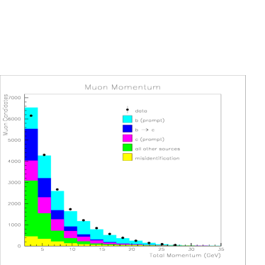
Figure 2: Total momentum distribution of identified muons in 1996-98 data (dots) and Monte Carlo (histogram).

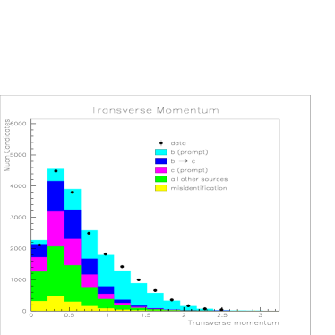
Figure 3: Transverse momentum distribution of identified muons in 1996-98 data (dots) amd Monte Carlo (histogram).

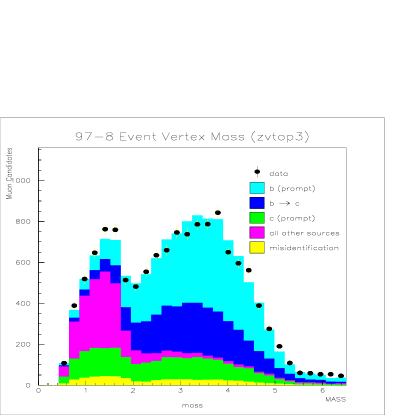
Figure 4: Event mass distribution for muons in 1996-8 data (dots) and Monte Carlo (histogram). The event mass is assumed to be the highest of the vertex masses found in the two hemispheres.

Figure 6: Distribution of $0.5\ln|p|$and $\sqrt{p_{T}}$ for muons in the 1996-98 data.

Figure 8: Electron NN output, $b\rightarrow{e}$ node.

Figure 9: Electron NN output, $b\rightarrow{c}\rightarrow{e}$ node.

Figure 10: Electron NN output, $c\rightarrow{e}$ node.

References

- [1] The LEP and SLD Collaborations, A combination pf preliminary electroweak measurements and constraints on the Standard Model, CERN-EP-2000-016 (2000).
- [2] G. Altarelli, N. Cabibbo, G. Corbó, L. Maiani and G. Martinelli, Nucl. Phys. B208, 365 (1982).
- [3] D. Jackson, Nucl. Instr. Meth. A388, 247 (1997).
- [4] SLD Collaboration, K. Abe et al., SLAC-PUB-7886 (1997)
- [5] T. Wright, SLD Analysis Note, March 2000
- [6] SLD Collaboration, K. Abe et al., SLAC-PUB-8200, (1999)
- [7] J. Fernandez, Ph.D. Thesis, University of California Santa Cruz, (1999).
- [8] G. Bellodi and G. Mancinelli, SLD Physics Note 75 (1999).
- [9] SLD Collaboration, K. Abe et al., Phys. Rev. Lett. 73, 25 (1994).
- [10] M. Fero et al., Nucl. Inst. Meth. A367, 111 (1995).
-
[11]
G. Agnew et al., SLAC-PUB-5906 (1992)
S. Hedges et al., SLAC-PUB-6950 (1995)
C. J. S. Damerell et al., Nucl. Inst. Meth. A400, 287 (1997). - [12] D. Axen et al., Nucl. Inst. Meth. A328, 472 (1993).
- [13] A. Benvenuti et al., Nucl. Inst. Meth. A276, 94 (1989); A290, 353 (1990).
- [14] SLD Design Report SLAC-273 UC-34D, May 1984, and revisions; D. Aston et al., SLAC-PUB-4795, Nucl. Inst. Meth. A283, 582 (1989); K. Abe et al., SLAC-PUB-5214, (1990).
- [15] SLD Collaboration, K. Abe et al., Nucl. Instr. and Meth. A371, 195 (1996).
- [16] W. Bartel et el., Z. Phys. C33, 23 (1986).
- [17] D. Falciai, SLD Physics Note 44, Dec. 1995.
- [18] T. Sjostrand, Comp. Phys. Comm. 82, 74 (1993).
- [19] N. Isgur, D. Scora, B. Grinstein, M. Wise, Phys. Rev. D39, 799 (1989); code provided by P. Kim and CLEO Collaboration.
- [20] Review of Particle Properties, Physical Review D50, 1173 (1994)
- [21] R. Wang, Ph.D. Thesis, Minnesota Univ., UMI-95-17404 (1994); B. Barich et al., PRL C76, 1570 (1996)
- [22] M. Thulasidas, PhD thesis, Syracuse University (1993)
- [23] W. Bacino et al., Phys. Rev. Lett. 43, 1073 (1979).
- [24] H. Albrecht et al., Z Phys. C58, 191 (1993).
- [25] GEANT 3.21 program, CERN Applications Software Group, CERN Program Library.
-
[26]
J.B. Stav and H.A. Olsen, Phys. Rev. D52,3, 1359 (1995)
J.B. Stav and H.A. Olsen, Phys. Rev. 54,1, 817 (1996). - [27] K. Abe et al., SLD Physics Note 66 (1997).
- [28] V. Ravindran and W. L. van Neerven, Phys. Lett. B445, 214 (1998).
- [29] Presentation of LEP Electroweak Heavy Flavour Results for Summer 1996 Conferences, LEPHF/96-01/
- [30] M. L. Swartz, hep-ex/9912026, to be published in the proceedings of International Symposium on Lepton and Photon Interactions at High Energies, Stanford University, August 9-14, 1999.