Measurement of the Angular Distribution of Electrons from $W\to e\nu$ Decays Observed in $p\bar{p}$ Collisions at $\sqrt{s}=1.8$ TeV

Abstract

We present the first measurement of the electron angular distribution parameter ${\alpha_{2}}$ in $W\to e\nu$ events produced in proton-antiproton collisions as a function of the $W$ boson transverse momentum. Our analysis is based on data collected using the DØ detector during the 1994–1995 Fermilab Tevatron run. We compare our results with next-to-leading order perturbative QCD, which predicts an angular distribution of ($1\pm\alpha_{1}\,\mathrm{cos}\theta^{*}+\alpha_{2}\,\mathrm{cos}^{2}\theta^{*}$), where $\theta^{*}$ is the polar angle of the electron in the Collins-Soper frame. In the presence of QCD corrections, the parameters $\alpha_{1}$ and $\alpha_{2}$ become functions of $p_{T}^{W}$, the $W$ boson transverse momentum. This measurement provides a test of next-to-leading order QCD corrections which are a non-negligible contribution to the $W$ boson mass measurement.

I Introduction

After the discovery of the $W$ boson [2, 3] at the CERN $p\overline{p}~{}$ collider, early studies of its properties verified its left-handed coupling to fermions and established it to be a spin 1 particle [4, 5]. These were accomplished through the measurement of the angular distribution of the charged lepton from the $W$ boson decay, a measurement ideally suited to $p\overline{p}~{}$colliders. The angular distribution was found to follow the well-known $V-A$ form $(1\pm\cos\theta^{*})^{2}$, where the polar angle $\theta^{*}$ is the lepton direction in the rest frame of the $W$ boson relative to the proton direction, and the sign is opposite that of the charge of the $W$ boson or emitted lepton; this formulation assumes that only valence quarks participate in the interaction, otherwise the angular distribution is slightly modified. It is important to note that these measurements were performed on $W$ bosons produced with almost no transverse momenta. This kinematic region is dominated by the production mechanism $\bar{q}+q^{\prime}\rightarrow W$. The center of mass energy used, $\sqrt{s}=540\,\mbox{GeV}$, is not high enough for other processes to contribute substantially.

At the higher energies of the Fermilab Tevatron ($\sqrt{s}=1.8\,\mbox{TeV}$) and higher transverse momenta explored using the DØ detector [6], other processes are kinematically allowed to occur. At low $W$ boson transverse momentum, $p_{T}^{W}$, the dominant higher order process involves initial state radiation of soft gluons. This process is calculated through the use of resummation techniques as discussed in Refs. [7, 8, 9, 10, 11, 12, 13]. At higher values of $p_{T}^{W}$, where perturbation theory holds, other processes contribute [14], such as:

1. $\bar{q}+q^{\prime}\rightarrow W+g$

2. $q+g\rightarrow W+q^{\prime}$

3. $g+g\rightarrow W+\bar{q}+q^{\prime}$

where only the first two contribute significantly at Tevatron energies [15]. These two processes change the form of the angular distribution of the emitted charged lepton to

$$\frac{d\sigma}{dp^{2}_{T}\,dy\,d\!\cos\theta^{*}}\propto(1\pm\alpha_{1}\cos\theta^{*}+\alpha_{2}\cos^{2}\theta^{*})$$ (1)

where the parameters $\alpha_{1}$ and $\alpha_{2}$ depend on the $W$ boson $p_{T}$ and rapidity, $y$ [15]. In Fig. 1, the parameters $\alpha_{1}$ and $\alpha_{2}$ are shown as functions of $p_{T}^{W}$. The angle $\theta^{*}$ is measured in the Collins-Soper frame [16]; this is the rest frame of the $W$ boson where the $z$-axis bisects the angle formed by the proton momentum and the negative of the antiproton momentum with the $x$-axis along the direction of $p_{T}^{W}$. This frame is chosen since it reduces the ambiguity of the neutrino longitudinal momentum to a sign ambiguity on $\cos\theta^{*}$.

In this paper, we present the first measurement of $\alpha_{2}$ as a function of $p_{T}^{W}$ [17], which serves as a probe of next-to-leading order quantum chromodynamics (NLO QCD), using the well-understood coupling between $W$ bosons and fermions. This measurement probes the effect of QCD corrections on the spin structure of $W$ boson production.

At DØ, the most precise $W$ boson mass measurement is made by fitting the transverse mass distribution. However, since the transverse mass of the $W$ boson is correlated with the decay angle of the lepton, the QCD effects discussed above introduce a systematic shift $\sim 40$ MeV to the $W$ boson mass measurement for events with $p_{T}^{W}\leq$ 15 GeV which must be taken into account. Presently, the Monte Carlo program used in the mass measurement models the angular distribution of the decay electron using the calculation of Mirkes [15]. During the next run of the Fermilab Tevatron collider (Run II), when the total error on the $W$ boson mass will be reduced from the current 91 MeV for DØ  [18, 19, 20, 21, 22, 23] to an estimated 50 MeV for 1 $\rm fb^{-1}$ and to about 30 MeV for 10 ${\rm fb}^{-1}$ [24], a good understanding of this systematic shift is important. Therefore, a direct measurement of the electron angular decay distribution is important to minimize the systematic error.

The paper is organized as follows: a brief description of the DØ detector is given in Sec. II, with an emphasis on the components used in this analysis. Event selection is discussed in Sec. III. The analysis procedure is described in Sec. IV. Finally, conclusions are presented in Sec. V.

FIG. 1.: The angular parameters $\alpha_{1}$ (dashed) and $\alpha_{2}$ (solid) as functions of $p_{T}^{W}$. These parameters are evaluated integrated over the $W$ boson rapidity, $y$. In the absence of QCD effects $\alpha_{1}$ and $\alpha_{2}$ equal 2.0 and 1.0, respectively.

II The DØ Detector

A Experimental Apparatus

The DØ detector, described in more detail elsewhere [6], is composed of four major systems. The innermost of these is a non-magnetic tracker used in the reconstruction of charged particle tracks. The tracker is surrounded by central and forward uranium/liquid-argon sampling calorimeters. These calorimeters are used to identify electrons, photons, and hadronic jets, and to reconstruct their energies. The calorimeters are surrounded by a muon spectrometer which is composed of an iron-core toroidal magnet surrounded by drift tube chambers. The system is used in the identification of muons and the reconstruction of their momenta. To detect inelastic $p$$\overline{p}~{}$ collisions for triggering, and to measure the luminosity, a set of scintillation counters is located in front of the forward calorimeters. For this analysis, the relevant components are the tracking system and the calorimeters. We use a coordinate system where the polar angle $\theta$ is measured relative to the proton beam direction $z$, and $\phi$ is the azimuthal angle. The pseudorapidity $\eta$ is defined as $-\ln(\tan\frac{\theta}{2})$, and $\rho$ is the perpendicular distance from the beam line.

The structure of the calorimeter has been optimized to distinguish electrons and photons from hadrons, and to measure their energies. It is composed of three sections: the central calorimeter (CC), and two end calorimeters (EC). The $\eta$-coverage for electrons used in this analysis is $\mid\eta\mid<1.1$ in the CC and $1.5<\mid\eta\mid<2.5$ for the EC. The calorimeter is segmented longitudinally into two sections, the electromagnetic (EM) and the hadronic (HAD) calorimeters. The primary energy measurement needed in this analysis comes from the EM calorimeter, which is subdivided longitudinally into four layers (EM1–EM4). The hadronic calorimeter is subdivided longitudinally into four fine hadronic layers (FH1–FH4) and one course hadronic layer (CH). The first, second and fourth layers of the EM calorimeter are transversely divided into cells of size $\Delta\eta\times\Delta\phi=0.1\times 0.1$. The shower maximum occurs in the third layer, which is divided into finer units of $0.05\times 0.05$ to improve the shower shape measurement.

B Trigger

The DØ trigger is built of three levels, with each level applying increasingly more sophisticated selection criteria on an event. The lowest level trigger, Level 0, uses the scintillation counters in front of the forward calorimeters to signal the presence of an inelastic $p\overline{p}~{}$ collision. Data from the Level 0 counters, the calorimeter and the muon chambers are sent to the Level 1 trigger, which allows the experiment to be triggered on total transverse energy, $E_{T}$, missing transverse energy, ${\hbox{$E$\kern-6.00006pt\lower-0.43057pt\hbox{/}}}_{T}$, $E_{T}$ of individual calorimeter towers, and/or the presence of a muon. These triggers operate in less than $3.5\;\mu\mbox{s}$, the time between bunch crossings. A few calorimeter and muon triggers require additional time, which is provided by a Level 1.5 trigger system.

Candidate Level 1 (and 1.5) triggers initiate the Level 2 trigger system that consists of a farm of microprocessors. These microprocessors run pared-down versions of the off-line analysis code to select events based on physics requirements. Therefore, the experiment can be triggered on events that have characteristics of $W$ bosons or other physics criteria.

III Particle Identification and Data Selection

This analysis relies on the DØ detector’s ability to identify electrons and the undetected energy associated with neutrinos. The particle identification techniques employed are described in greater detail in Ref. [25]. The following sections provide a brief summary of the techniques used in this paper.

A Electron Identification

Identification of electrons starts at the trigger level, where clusters of electromagnetic energy are selected. At Level 1, the trigger searches for EM calorimeter towers ($\Delta\phi\times\Delta\eta=0.1\times 0.1$) that exceed predefined thresholds. $W$ boson triggers require that the energy deposited in a single EM calorimeter tower exceed 10 GeV. Those events that satisfy the Level 1 trigger are processed by the Level 2 filter. The trigger towers are combined with energy in the surrounding calorimeter cells within a window of $\Delta\phi\times\Delta\eta=0.3\times 0.3$. Events are selected at Level 2 if the transverse energy in this window exceeds 20 GeV. In addition to the $E_{T}$ requirement, the longitudinal and transverse shower shapes are required to match those expected for electromagnetic showers. The longitudinal shower shape is described by the fraction of the energy deposited in each of the four EM layers of the calorimeter. The transverse shower shape is characterized by the energy deposition patterns in the third EM layer. The difference between the energies in concentric regions covering $0.25\times 0.25$ and $0.15\times 0.15$ in $\eta\times\phi$ must be consistent with that expected for an electron [6].

In addition, at Level 2, the energy cluster isolation is required to satisfy $f_{iso}<0.15$, where $f_{iso}$ is defined as:

$$f_{iso}=\frac{E_{{\rm total}}(0.4)-E_{{\rm EM}}(0.2)}{E_{{\rm EM}}(0.2)},$$ (2)

$E_{{\rm total}}(0.4)$ is the total energy, and $E_{{\rm EM}}(0.2)$ the electromagnetic energy, in cones of $R=\sqrt{(\Delta\eta)^{2}+(\Delta\phi)^{2}}=0.4$ and $0.2$, respectively. This cut preferentially selects the isolated electrons expected from vector boson decay.

Having selected events with isolated electromagnetic showers at the trigger level, a set of tighter cuts is imposed off-line to identify electrons, thereby reducing the background from QCD multijet events. The first step in identifying an electron is to build a cluster about the trigger tower using a nearest neighbor algorithm. As at the trigger level, the cluster is required to be isolated ($f_{iso}<0.15$). To increase the likelihood that the cluster is due to an electron and not a photon, a track from the central tracking system is required to point at its centroid. We extrapolate the track to the third EM layer in the calorimeter and calculate the distance between the extrapolated track and the cluster centroid in the azimuthal direction, $\rho\Delta\phi$, and in the $z$-direction, $\Delta z$. The cluster centroid position is extracted at the radius of the third EM layer of the calorimeter, $\rho$. The $z$ position of the event vertex is defined by the line connecting the center of gravity calorimeter position of the electron and the center of gravity of its associated track in the central tracking system, extrapolated to the beamline. The electron $E_{T}$ is calculated using this vertex definition [25]. The variable

$$\sigma_{trk}^{2}=\left(\frac{\rho\Delta\phi}{\sigma_{\rho\phi}}\right)^{2}+\left(\frac{\Delta z}{\sigma_{z}}\right)^{2}$$ (3)

where $\sigma_{\rho\phi}$ and $\sigma_{z}$ are the respective track resolutions, quantifies the quality of the match. A cut of $\sigma_{trk}<5$ is imposed on the data. Electromagnetic clusters that satisfy these criteria, referred to as “loose electrons,” are then subjected to a 4-variable likelihood test previously used in the measurement of the top quark mass by the DØ collaboration [26]. The four variables are:

• A $\chi^{2}$ comparison of the shower shape with the expected shape of an electromagnetic shower, computed using a $41$-variable covariance matrix [27] of the energy depositions in the cells of the electromagnetic calorimeter and the event vertex.

• The electromagnetic energy fraction, which is defined as the ratio of shower energy in the EM section of the calorimeter to the total EM energy plus the energy in the first hadronic section of the calorimeter.

• A comparison of track position to cluster centroid position as defined in Eq. 3.

• The ionization, $dE/dx$, along the track, to reduce contamination from $e^{+}e^{-}$ pairs due to photon conversions. This variable is effective in reducing the background from jets fragmenting into neutral pions which then decay into photon pairs.

To a good approximation, these four variables are independent of each other for electron showers. Electrons that satisfy this additional cut are called “tight” electrons.

B Missing Energy

The primary sources of missing energy in an event include the neutrinos that pass through the calorimeter undetected and the apparent energy imbalance due to calorimeter resolution. The energy imbalance is measured only in the transverse plane due to the unknown momenta of the particles escaping within the beam pipes.

The missing transverse energy is calculated by taking the negative of the vector sum of the transverse energy in all of the calorimeter cells. This gives both the magnitude and direction of the ${\hbox{$E$\kern-6.00006pt\lower-0.43057pt\hbox{/}}}_{T}$, allowing the calculation of the transverse mass of the $W$ boson candidates, $M_{T}^{W}$, given by

$$M_{T}^{W}=\sqrt{2E_{T}^{e}\mbox{${\hbox{$E$\kern-6.00006pt\lower-0.43057pt\hbox{/}}}_{T}$}[1-\cos(\phi^{e}-\phi^{\nu})]}$$ (4)

in which $E_{T}^{e}$ is the transverse energy of the electron and $\phi^{e}$ and $\phi^{\nu}$ are the azimuthal angles of the electron and neutrino, respectively.

C Event Selection

The $W$ boson data sample used in this analysis was collected during the 1994–1995 run of the Fermilab Tevatron collider. This data sample corresponds to an integrated luminosity of $85.0\pm 3.6\;\rm pb^{-1}$. Events are selected by requiring one tight electron in the central calorimeter $(\mid\eta\mid<1.1)$ with $E_{T}$ $>25$ GeV. The CC consists of 32 $\phi$ modules. To avoid areas of reduced response between neighboring modules, the $\phi$ of an electron is required to be at least $0.05\times 2\pi/32$ radians away from the position of a module boundary. In addition, events are required to have ${\hbox{$E$\kern-6.00006pt\lower-0.43057pt\hbox{/}}}_{T}$ $>25$ GeV. If there is a second electron in the event (loose or tight) and the dielectron invariant mass $M_{ee}$ is close to the $Z$ boson mass ($75\;\mbox{GeV}<M_{ee}<105\;\mbox{GeV}$), the event is rejected.

To ensure a well-understood calorimeter response and to reduce luminosity-dependent effects, two additional requirements are imposed. The Main Ring component of the Tevatron accelerator passes through the outer part of the hadronic calorimeter. Beam losses from the Main Ring can cause significant energy deposits in the calorimeter, resulting in false ${\hbox{$E$\kern-6.00006pt\lower-0.43057pt\hbox{/}}}_{T}$. The largest losses occur when beam is injected into the Main Ring. Events occurring within a 400 ms window after injection are rejected, resulting in a 17% loss of data. Large beam losses can also occur when particles in the Main Ring pass through the DØ detector. Hence we reject events within a 1.6 $\mu\rm{s}$ window around these occurrences, resulting in a data loss of approximately $8\%$. After applying all of the described cuts, a total of 41173 $W$ boson candidates is selected using electrons found in the central calorimeter.

IV Experimental Method

A Monte Carlo Simulation

For this analysis, a Monte Carlo program with a parameterized detector simulation is used. This is the same Monte Carlo used in our previous results on the $W$ boson mass measurement [20] and the inclusive cross sections of the $W$ and $Z$ bosons [25], so it will only be briefly summarized here.

In the Monte Carlo, the detector response is parameterized using the data from the experiment. This includes using $Z$ bosons and their hadronic recoil to study the response and resolution. The response itself is then parameterized as a function of energy and angle.

The kinematic variables for each $W$ boson are generated using the resbos [13] event generator with the theoretical model described in Refs. [11, 14], and the CTEQ4M parton distribution functions (pdf’s) [28]. Finally, the angular distribution is generated according to the calculation of Mirkes [15].

1 Hadronic Scale

One of the parameters needed for the Monte Carlo program used in this study is the response of the calorimeter to the hadronic recoil, defined as the sum of all calorimeter cells excluding the cells belonging to the electron. The detector response and resolution for particles recoiling against a $W$ boson should be the same as for particles recoiling against a $Z$ boson. For $Z\rightarrow ee$ events, we measure the transverse momentum of the $Z$ boson from the $e^{+}e^{-}$ pair, $p_{T}^{~{}ee}$, and from the recoil jet momentum, $p_{T}^{~{}\rm rec}$, in the same manner as for $W\rightarrow e\nu$ events. By comparing $p_{T}^{~{}ee}$ and $p_{T}^{~{}\rm rec}$, the recoil response is calibrated relative to the well-understood electron response [20].

The recoil momentum is carried by many particles, mostly hadrons, with a wide momentum spectrum. Since the response of calorimeters to hadrons tends to be non-linear and the recoil particles are distributed over the entire calorimeter, including module boundaries with reduced response, we expect a momentum-dependent response function with values below unity.

To measure the recoil response from our data, we use a sample of $Z$ boson events with one electron in the CC and the second in the CC or the EC (CC/CC+EC). This allows the rapidity distribution of the $Z$ bosons to approximate that of the $W$ bosons where the neutrinos could be anywhere in the detector. Further, we require that both electrons satisfy the tight electron criteria. This reduces the background for the topology where one electron is in the EC. We project the transverse momenta of the recoil and the $Z$ boson onto the inner bisector of the electron directions ($\eta$-axis), as shown in Fig. 2. By projecting the momenta onto an axis that is independent of any energy measurement, noise contributions to the momenta average to zero and do not bias the result.

To determine the functional dependence of the recoil system with respect to the dielectron system, $\vec{p}_{T}^{~{}\rm rec}\cdot(-\hat{\eta})$ is plotted as a function of $\vec{p}_{T}^{~{}ee}\cdot\hat{\eta}$ as shown in Fig. 3. For $p_{T}^{ee}>10$ GeV, the hadronic response is well described by a linear scale and offset:

$$\vec{p}_{T}^{~{}\rm rec}\cdot\hat{\eta}=\alpha_{H}\;\vec{p}_{T}^{~{}ee}\cdot\hat{\eta}+\beta_{H}$$ (5)

The parameters $\alpha_{H}$ and $\beta_{H}$ are calculated using a least-squares fit to the data in the region ${p}_{T}^{ee}>5\;{\rm GeV}$, resulting in $\alpha_{H}=0.972\pm 0.0095$ and $\beta_{H}=(-1.21\pm 0.14)\;{\rm GeV}$. For small values of $p_{T}^{ee}$, $p_{T}^{ee}<10$ GeV, the relation between the hadronic and electronic recoil is best described by a logarithmic function [20, 29]:

$$\vec{p}_{T}^{~{}\rm rec}\cdot\hat{\eta}=\left(\gamma_{H}\ln(\vec{p}_{T}^{~{}ee}\cdot\hat{\eta})+\delta_{H}\right)\vec{p}_{T}^{~{}ee}\cdot\hat{\eta}$$ (6)

The parameters $\gamma_{H}$ and $\delta_{H}$ are derived using a least-squares fit to the data in the region $p_{T}^{ee}<10\;{\rm GeV}$ (see Fig. 4), yielding $\gamma_{H}=0.099\pm 0.019$ and $\delta_{H}=0.620\pm 0.047$. In the intermediate region, $5\;{\rm GeV}<p_{T}^{ee}<10\;{\rm GeV}$, the logarithmic and the linear fit match.

FIG. 2.: Definition of the $\eta$–$\xi$ coordinate system in a $Z$ boson event. $\vec{e}_{t}^{~{}i}$ denote the transverse momentum vectors of the two electrons. The $\eta$ axis is the bisector of the electrons in the transverse plane; the $\xi$ axis is perpendicular to $\eta$ [20].

FIG. 3.: For $Z\rightarrow ee$ events (points) the average value of $\vec{p}_{T}^{~{}\rm rec}\cdot(-\hat{\eta})$ is shown versus $\vec{p}_{T}^{~{}ee}\cdot\hat{\eta}$. The line shown is obtained from a linear least squares fit to the data above $p_{T}^{ee}$ = 5 GeV as described in the text. The dotted lines represent the statistical uncertainties from the fit.

FIG. 4.: For $Z\rightarrow ee$ events (points) the average value of $\vec{p}_{T}^{~{}\rm rec}\cdot(-\hat{\eta})$ is shown versus $\vec{p}_{T}^{~{}ee}\cdot\hat{\eta}$. Shown is the linear fit valid at $p_{T}^{ee}>$ 10 GeV and a logarithmic fit valid for $p_{T}^{ee}<10$ GeV. The dotted lines represent the statistical uncertainties from the linear fit.

2 Tuning the Recoil Resolution Parameters

In the Monte Carlo, we parameterize the calorimeter resolution, $\sigma_{\rm rec}$, for the hard component of the recoil as

$$\sigma_{\rm rec}=s_{\rm rec}\sqrt{p_{T}^{~{}\rm rec}}$$ (7)

where $s_{\rm rec}$ is a tunable parameter, and $p_{T}^{~{}\rm rec}$ is the recoil momentum of the hard component.

The soft component of the recoil is modeled by the transverse momentum imbalance from minimum bias events. This automatically models detector resolution and pile-up. To account for any possible difference between the underlying event in $W$ boson events and minimum bias events, we multiply the minimum bias ${\hbox{$E$\kern-6.00006pt\lower-0.43057pt\hbox{/}}}_{T}$ by a correction factor $\alpha_{\rm mb}$. We tune the two parameters $s_{\rm rec}$ and $\alpha_{\rm mb}$ by comparing the width of the $\eta$-balance, $\vec{p}_{T}^{~{}\rm rec}\cdot\hat{\eta}/R_{\rm rec}+\vec{p}_{T}^{~{}ee}\cdot\hat{\eta}$, measured from the CC/CC+EC $Z$ boson data sample to Monte Carlo and adjusting the parameters in the Monte Carlo simultaneously until the widths agree. The width of the $\eta$-balance is a measure of the recoil momentum resolution. The recoil response, $R_{\rm rec}$, is defined as

$$R_{\rm rec}=\frac{|\vec{p}_{T}^{~{}\rm rec}\cdot\hat{q}_{T}|}{|q_{T}|},$$ (8)

where $q_{T}$ is the generated transverse momentum of the $Z$ boson. The contribution of the electron momentum resolution to the width of the $\eta$-balance is negligibly small. The contribution of the recoil momentum resolution grows with $\vec{p}_{T}^{~{}ee}\cdot\hat{\eta}$ while the contribution from the minimum bias ${\hbox{$E$\kern-6.00006pt\lower-0.43057pt\hbox{/}}}_{T}$ is independent of $\vec{p}_{T}^{~{}ee}\cdot\hat{\eta}$. This allows us to determine $s_{{\rm rec}}$ and $\alpha_{\rm mb}$ simultaneously and without sensitivity to the electron resolution by comparing the width of the $\eta$-balance predicted by the Monte Carlo model with that observed in the data in bins of $\vec{p}_{T}^{~{}ee}\cdot\hat{\eta}$. We perform a $\chi^{2}$ fit comparing Monte Carlo and collider data. The values that minimize the $\chi^{2}$ are found to be $s_{{\rm rec}}=0.665\pm 0.062\;{\rm GeV^{1/2}}$ and $\alpha_{{\rm mb}}=1.095\pm 0.020$. The non-linear hadronic scale in the region $p_{T}<$10 GeV leads to $s_{{\rm rec}}=0.50\pm 0.06\;{\rm GeV^{1/2}}$, while $\alpha_{{\rm mb}}$ is unchanged.

B Extraction of the Lepton Angle

Since only the transverse components of the neutrino momentum are measured, the transformation from the lab frame to the $W$ boson rest frame (Collins-Soper frame) is not directly calculable. Therefore the polar angle of the electron from the $W$ boson decay, $\theta^{*}$, is not directly measurable. In this analysis, $\theta^{*}$ is inferred from the correlation between the transverse mass of the $W$ boson and $\cos\theta^{*}$ through the use of Bayes’ Theorem[30].

Experimentally, the only information we have about the $W$ boson is that contained in the two kinematic variables $M_{T}^{W}$ and $p_{T}^{W}$. But $M_{T}^{W}$ depends on the polar angle $\cos\theta^{*}$, the azimuthal angle $\phi^{*}$ over which we have integrated, and $p_{T}^{W}$. Therefore, the two experimentally measured variables $M_{T}^{W}$ and $p_{T}^{W}$ give $\cos\theta^{*}$. An analytic expression exists for this relation (see Ref. [31]), so in principle the equation is solvable for $\cos\theta^{*}$, but the experimental values of both $M_{T}^{W}$ and $p_{T}^{W}$ include detector resolution effects that have to be unfolded to give the true $\cos\theta^{*}$ distribution. Even with perfect detector resolution, the equation would only be solvable if the $W$ boson mass was known on an event by event basis. Therefore, we calculate the probability of measuring $M_{T}^{W}$ for a given value $\cos\theta^{*}$ in a given $p_{T}^{W}$ bin, $p(M_{T}^{W}|\cos\theta^{*},p_{T}^{W})$. This probability function is inverted to give the probability of measuring $\cos\theta^{*}$ for a measured $M_{T}^{W}$, $p(\cos\theta^{*}|M_{T}^{W},p_{T}^{W})$, using Bayes’ Theorem:

$$p(\cos\theta^{*}|M_{T}^{W},p_{T}^{W})=\frac{p(M_{T}^{W}|\cos\theta^{*},p_{T}^{W})p(\cos\theta^{*})}{\int p(M_{T}^{W}|\cos\theta^{*},p_{T}^{W})p(\cos\theta^{*})d\cos\theta^{*}}$$ (9)

where $p(\cos\theta^{*})$ is the prior probability function, which we take as $p(\cos\theta^{*})=(1+\cos^{2}\theta^{*})$, the charge-averaged expectation from $V-A$ theory without QCD corrections.

To derive the probability function $p(M_{T}^{W}|\cos\theta^{*},p_{T}^{W})$, we use a Monte Carlo simulation of the DØ detector, which is described in Sec. IV A. The correlation between $M_{T}^{W}$ and $\cos\theta^{*}$ for $p_{T}^{W}\leq 10\,\mbox{GeV}$ is shown in Fig. 5. After determining $p(M_{T}^{W}|\cos\theta^{*},p_{T}^{W})$, it is inverted, yielding $p(\cos\theta^{*}|M_{T}^{W},p_{T}^{W})$. The angular distribution is calculated by multiplying $p(\cos\theta^{*}|M_{T}^{W},p_{T}^{W})$ with the measured transverse mass distribution. This is done in four $p_{T}^{W}$ bins covering 0–10 GeV, 10–20 GeV, 20–35 GeV, and 35–200 GeV.

With the unfolded angular distributions now calculated, the value of $\alpha_{2}$ in each of the four $p_{T}^{W}$ bins can be determined. This is accomplished by generating a set of angular distribution templates for different values of $\alpha_{2}$. These templates are generated in a series of Monte Carlo experiments using the Monte Carlo program described in Sec. IV A.

The $\cos\theta^{*}$ templates are compared to the data through the use of a maximum likelihood method. Fig. 6 shows a series of angular distribution templates for different values of $\alpha_{2}$ and $p_{T}^{W}<10\,\mbox{GeV}$.

FIG. 5.: Smeared $W$ boson transverse mass versus true $\cos\theta^{*}$ for $p_{T}^{W}\leq$ 10 GeV from Monte Carlo. Acceptance cuts have been applied to events in this plot. This correlation plot is used to infer the $\cos\theta^{*}$ distribution from the measured $M_{T}^{W}$ distribution.

FIG. 6.: Templates of the angular distribution for various $\alpha_{2}$ values for $p_{T}^{W}\leq$ 10 GeV. These templates are obtained from Monte Carlo after acceptance cuts have been applied which results in the drop-off at small angles. Each template is normalized to unity.

1 The Treatment of $\alpha_{1}$

Since there is no magnetic field in the central charged particle tracking detector, it is not possible to identify the charge of the electron. Without charge identification, this analysis can only be performed by summing over the $W$ boson charge and polarization. This implies that the linear term in $\cos\theta^{*}$ averages to zero in the limit of complete acceptance. However, after acceptance cuts have been applied, even the charge averaged angular distribution does depend on the linear term. The reason is that events generated with a non-zero $\alpha_{1}$ correspond to slightly more central electrons after they are boosted into the lab frame compared to events generated with $\alpha_{1}$ set to zero. After acceptance cuts have been applied, fewer events are lost at large $\cos\theta^{*}$. However, since this is only a second order effect, this measurement is not sensitive to $\alpha_{1}$. For this analysis, we calculate $\alpha_{1}$ [15] based on the measured $p_{T}^{W}$of each event. Possible variations of $\alpha_{1}$ are treated as a source of systematic uncertainty (see Sec. IV E).

C Backgrounds

To extract the electron angular distribution from the transverse mass distribution, the size of the backgrounds has to be estimated. The backgrounds are estimated as functions of the $W$ boson transverse momentum and transverse mass, these being the two variables used to extract the angular distribution. The following sections describe how the four dominant backgrounds are calculated, and how they depend on transverse mass and transverse momentum.

1 QCD

A large potential source of background is due to QCD dijet events, where one jet is misidentified as an electron and the energy in the event is mismeasured resulting in large ${\hbox{$E$\kern-6.00006pt\lower-0.43057pt\hbox{/}}}_{T}$. This background is estimated using QCD multijet events from our data following the procedure described in detail in Ref. [25]. Briefly, the fraction of QCD background events in the $W$ boson sample is given by

$$f_{QCD}^{W}=\frac{\epsilon_{j}}{N_{t}}\left(\frac{\epsilon_{s}N_{\ell}-N_{t}}{\epsilon_{s}-\epsilon_{j}}\right)$$ (10)

with the following variables: $N_{\ell}$ and $N_{t}$ are the number of events in the $W$ sample satisfying loose and tight electron criteria, respectively. The tight electron efficiency, $\epsilon_{s}$, is the fraction of loose electrons passing tight cuts as found in a sample of $Z$ boson events, where one electron is required to pass tight electron identification cuts and the other serves as an unbiased probe for determining relative efficiencies. The jet efficiency, $\epsilon_{j}$, is the fraction of loose “fake” electrons that pass tight electron cuts in a sample of multijet events. This sample is required to have low ${\hbox{$E$\kern-6.00006pt\lower-0.43057pt\hbox{/}}}_{T}$($<15\,\mbox{GeV}$) to minimize the number of $W$ bosons in the sample. From this analysis, the overall QCD background fraction is found to be $f_{QCD}^{W}=(0.77\pm 0.6)\%\>$ with a transverse mass cut of $50<M_{T}^{W}<90$ GeV imposed, this being the range used in the Bayesian analysis. For $f_{QCD}^{W}$ as a function of $p_{T}^{W}$, see Table I.

2 $Z\rightarrow ee$

Another source of background is $Z$ boson events in which one electron is lost in a region of the detector that is uninstrumented or one that has a lower electron finding efficiency such as that between the CC and the EC. This results in a momentum imbalance, with the event now being indistinguishable from a $W$ boson event. This background can only be estimated using Monte Carlo $Z$ boson events. The number of such $Z$ boson events present in the $W$ boson sample is calculated by applying the $W$ boson selection cuts to herwig [32] $Z\rightarrow ee$ events that are processed through a geant [33] based simulation of the DØ detector and then overlaid with events from random $p$$\overline{p}~{}$ crossings. This is done to simulate the underlying event, so that the effect of the luminosity can be included. The overall background fraction is found to be $f_{Z}^{W}=(0.50\pm 0.06)\%$ averaged over all $p_{T}^{W}$. For the background fraction in each $p_{T}^{W}$ bin, see Table I.

3 $t\overline{t}~{}$Production

The top quark background is not expected to contribute significantly, except in the highest $p_{T}^{W}$ bin. The background from these events comes from $t$ quarks decaying to $W$ bosons. If one $W$ boson decays electronically while the other decays into two hadronic jets, the event can mimic a high $p_{T}$ $W$ boson event. This background, like the $Z$ boson background, is calculated from Monte Carlo using herwig $t$$\overline{t}~{}$events. The overall background fraction is $f_{t\overline{t}}^{W}=(0.087\pm 0.027)\%$. For the background fraction in each $p_{T}^{W}$ bin, see Table I.

4 $W\rightarrow\tau\nu$

$W\rightarrow\tau\nu$ events in which the $\tau$ decays into an electron and two neutrinos are indistinguishable from $W\rightarrow e\nu$ events. This background is estimated from Monte Carlo simulations using the $W$ boson mass Monte Carlo described above. A fraction of the events is generated as $W\rightarrow\tau\nu$, decayed electronically, with acceptance and fiducial cuts applied to the decay electron in the same manner as in $W\rightarrow e\nu$ events. The acceptance for $W\rightarrow\tau\nu\rightarrow e\nu\nu\nu$ is reduced by the branching fraction $B(\tau\rightarrow e\nu\nu)=(17.81\pm 0.07)\%$ [34]. The kinematic acceptance is further reduced by the $E_{T}$ cut on the electron since the three-body decay of the $\tau$ leads to a very soft electron $E_{T}$ spectrum compared to that from $W\rightarrow e\nu$ events (see Fig. 7). The fraction of $W\rightarrow\tau\nu\rightarrow e\nu\nu\nu$ events after these cuts are applied to the Monte Carlo is $f^{W}_{\tau}=(2.03\pm 0.19)\%$ over all $p^{W}_{T}$.

For this analysis, the angular ($\cos\theta^{*}$) templates are generated using the $W$ boson mass Monte Carlo simulator with the branching ratio $B(W\rightarrow\tau\nu)=B(W\rightarrow e\nu)$, assuming lepton universality, and the above value for $B(\tau\rightarrow e\nu\nu)$. The transverse mass of $W\rightarrow\tau\nu$ events (Fig. 8) is on average lower than that of $W\rightarrow e\nu$ events, due to the three-body decay of the $\tau$.

FIG. 7.: Electron $E_{T}$ spectrum for Monte Carlo $W\rightarrow\tau\nu\rightarrow e\nu\nu\nu$ events (dashed) and $W\rightarrow e\nu$ events (solid histogram). Both spectra are normalized to unity for shape comparison.

FIG. 8.: Transverse mass distribution for $W\rightarrow e\nu$ events (solid) and $W\rightarrow\tau\nu\rightarrow e\nu\nu\nu\>$ events (dashed) from Monte Carlo.

5 Summary of Backgrounds

As we have shown in the previous sections, and as can be clearly seen in Fig. 9, the background fractions in this measurement are small (a few per cent) over all $M_{T}^{W}$ and $p_{T}^{W}$ ranges. The dominant backgrounds are due to QCD multijet events and $Z$ boson decays, except in the highest $p_{T}^{W}$ bin where the $t\bar{t}$ background is comparable in size.

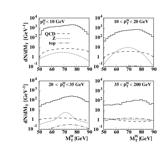
FIG. 9.: Transverse mass spectrum for $W\rightarrow e\nu$ candidate events (solid histogram) and QCD (dashed), $Z$ boson (dotted), and $t$$\overline{t}~{}$ backgrounds (dashed-dotted) in four $p_{T}^{W}$ bins.

$p_{T}^{W}$ [GeV]	$f_{QCD}^{W}\;[\%]$	$f_{Z}^{W}\;[\%]$	$f_{t\overline{t}}^{W}\;[\%]$
0–10	$0.6\pm 1.0$	$0.16\pm 0.02$	$0.0028\pm 0.0009$
10–20	$1.0\pm 1.0$	$1.1\pm 0.1$	$0.025\pm 0.008$
20–35	$1.3\pm 1.0$	$1.4\pm 0.2$	$0.15\pm 0.05$
35–200	$2.0\pm 1.1$	$1.7\pm 0.2$	$2.0\pm 0.6$

TABLE I.: Background fractions as a function of $p_{T}^{W}$ for events with a transverse mass cut of $50<M_{T}^{W}<90$ GeV imposed.

D The Measurement of $\alpha_{2}$

To obtain the angular distribution for $W$ boson events from data, the transverse mass distribution is inverted through the use of Bayes’ Theorem as described in Sec. IV B. Since the probability distribution function used to invert the $M_{T}^{W}$ distribution is generated from Monte Carlo, we compare the background-subtracted $M_{T}^{W}$ distribution from data to that generated through our Monte Carlo to verify that it models the physics and detector correctly (see Fig. 10). Based on a $\chi^{2}$ test, the agreement between data and Monte Carlo is good; the $\chi^{2}$-probabilities are $11.2\%$, $80.6\%$, $93.7\%$ and $53.7\%$ in order of increasing $p_{T}^{W}$ bins. Likewise, the experimental and Monte Carlo $p_{T}^{W}$ distributions can be compared, with the two showing agreement with a $\chi^{2}$-probability of $7.4\%$, where only statistical errors are taken into account (see Fig. 11).

After extracting the angular distribution, the parameter $\alpha_{2}$ is computed using the method of maximum likelihood (see Fig. 12). The angular distribution is compared to a series of Monte Carlo generated templates, each with a different value of $\alpha_{2}$. The template that results in the maximum likelihood gives the value of $\alpha_{2}$ for each $p_{T}^{W}$ bin (Fig. 13). The $1\sigma$ uncertainties in $\alpha_{2}$ are approximately given by the points where the log-likelihood drops by 0.5 units. To estimate the goodness of fit, the measured angular distributions are compared to these templates using a $\chi^{2}$ test. The $\chi^{2}$-probabilities that we obtain are $8.4\%$, $59.1\%$, $87.7\%$ and $11.6\%$ in order of increasing $p_{T}^{W}$ bins.

FIG. 10.: Background subtracted transverse mass distributions (crosses) in four $p_{T}^{W}$ bins compared to Monte Carlo predictions (solid histograms).

FIG. 11.: Background subtracted transverse momentum distribution (crosses) compared to Monte Carlo prediction (solid histogram). The error bars indicate statistical uncertainties only.

FIG. 12.: Log-likelihood functions for four different $p_{T}^{W}$ bins. The arrows denote the values of maximum likelihood and the $1\sigma$ errors. The vertical lines labeled $V-A$ show $\alpha_{1}=1$, the value for $V-A$ theory without QCD corrections.

   

   

FIG. 13.: Angular distributions for data compared to Monte Carlo templates for four different $p_{T}^{W}$ bins. Shown are the templates that fit best (solid) and the templates for $\alpha_{2}$ = 1 (dashed) and $\alpha_{2}$ = 0 (dotted).

E Systematic Errors

Systematic errors on our measurement of $\alpha_{2}$ are due to uncertainties in the backgrounds and the parameters used to model the detector in the Monte Carlo. To estimate the errors due to the background uncertainties, the parameters from fits of the transverse mass distributions of the background are varied within their errors, and the analysis is repeated. For the errors due to detector modeling, the corresponding Monte Carlo parameters are varied within their errors and the analysis is repeated with new angular templates. For this analysis, we fixed $\alpha_{1}$ to the values given by the next-to-leading order QCD prediction (see Fig. 1). The error associated with this choice is estimated by changing $\alpha_{1}$ to the value calculated in the absence of QCD effects ($\alpha_{1}=2.0$).

The dominant systematic errors are due to uncertainties in the electromagnetic energy scale and the QCD background. All systematic errors are summarized in Table II. The systematic errors are combined in quadrature. The statistical uncertainties are, except for the first $p_{T}^{W}$ bin, larger by a factor of three than the systematic uncertainties.

$p_{T}^{W}$ [GeV]	$0-10$	$10-20$	$20-35$	$35-200$
$\alpha_{2},\>measured$	$1.09$	$0.84$	$0.52$	$0.13$
stat. errors	$\pm 0.13$	$\pm 0.25$	$\pm 0.36$	$\pm 0.38$
$\alpha_{2},\>predicted$	$0.98$	$0.89$	$0.68$	$0.24$
mean $p_{T}^{W}$	5.3	13.3	25.7	52.9
QCD	$\pm 0.04$	$\pm 0.05$	$\pm 0.09$	$\pm 0.07$
$Z\rightarrow ee$	$\pm 0.01$	$\pm 0.02$	$\pm 0.02$	$\pm 0.04$
$t\overline{t}~{}$	$\pm 0.00$	$\pm 0.00$	$\pm 0.00$	$\pm 0.02$
EM scale	$\pm 0.06$	$\pm 0.05$	$\pm 0.03$	$\pm 0.04$
hadronic scale	$\pm 0.03$	$\pm 0.01$	$\pm 0.04$	$\pm 0.04$
hadronic resol.	$\pm 0.02$	$\pm 0.02$	$\pm 0.05$	$\pm 0.06$
fixed $\alpha_{1}$	$\pm 0.01$	$\pm 0.05$	$\pm 0.03$	$\pm 0.03$
combined syst.	$\pm 0.08$	$\pm 0.09$	$\pm 0.12$	$\pm 0.12$

TABLE II.: Central values for $\alpha_{2}$ with statistical and systematic errors.

F Results and Sensitivity

To estimate the sensitivity of this experiment, the $\chi^{2}\>$ of the $\alpha_{2}$ distribution is calculated with respect to the prediction of the $V-A$ theory modified by next-to-leading order QCD and that of the $V-A$ theory in the absence of QCD corrections. The $\chi^{2}\>$ with respect to the QCD prediction is 0.8 for 4 degrees of freedom, which corresponds to a probability of $94\%$. The $\chi^{2}\>$ with respect to pure $V-A$ is 7.0 for 4 degrees of freedom, which corresponds to $14\%$ probability. To make a more quantitative estimate of how much better $V-A$ modified by next-to-leading order QCD agrees over pure $V-A$, we use the odds-ratio method , which prefers the former over the latter theory by $\approx 2.3\,\sigma$. The results of our measurement along with the theoretical prediction are given in Fig. 14 and Table II.

FIG. 14.: Measured $\alpha_{2}$ as a function of $p_{T}^{W}$ compared to the next-to-leading order QCD calculation by Mirkes (curve) and calculation in the absence of QCD (horizontal line). The combined systematic and statistical errors are shown as vertical bars, while the statistical errors alone are marked by horizontal ticks.

V Conclusions

Using data taken with the DØ detector during the 1994–1995 Fermilab Tevatron collider run, we have presented a measurement of the angular distribution of decay electrons from $W$ boson events. A next-to-leading order QCD calculation is preferred by $\approx 2.3\,\sigma$ over a calculation where no QCD effects are included.

VI Acknowledgments

We thank the staffs at Fermilab and at collaborating institutions for contributions to this work, and acknowledge support from the Department of Energy and National Science Foundation (USA), Commissariat à L’Energie Atomique and CNRS/Institut National de Physique Nucléaire et de Physique des Particules (France), Ministry for Science and Technology and Ministry for Atomic Energy (Russia), CAPES and CNPq (Brazil), Departments of Atomic Energy and Science and Education (India), Colciencias (Colombia), CONACyT (Mexico), Ministry of Education and KOSEF (Korea), CONICET and UBACyT (Argentina), A.P. Sloan Foundation, and the A. von Humboldt Foundation.

REFERENCES

- [1]
- [2] UA1 Collaboration, G. Arnison et al., Phys. Lett. B122, 103 (1983).
- [3] UA2 Collaboration, G. Bonner et al., Phys. Lett B122, 476 (1983); UA2 Collaboration, K. Borer et al., Helv. Phys. Acta 57, 290 (1984).
- [4] UA1 Collaboration, G. Arnison et al., Phys. Lett. B166, 484 (1986); UA1 Collaboration, C. Albajar et al., Z. Phys. C 44, 15 (1989).
- [5] E. Locci, in Proc. 8th European Symp. on Nucleon-Antinucleon Interactions: Antiproton 86, Thessaloniki, edited by S. Charalambous, C. Papastefanou, and P. Pavlopoulos (World Scientific, Signapore, 1987).
- [6] DØ Collaboration, S. Abachi et al., Nucl. Instrum. Methods in Phys. Res. A 338, 185 (1994).
- [7] J.C. Collins and D.E. Soper, Nucl. Phys. B193, 381 (1981); B213, 545(E) (1983); J.C. Collins, D.E. Soper, and G. Sterman, ibid. B250, 199 (1985).
- [8] C.T.H. Davies and W.J. Stirling, Nucl. Phys. B244, 337 (1984).
- [9] G. Altarelli, R.K. Ellis, M. Greco, and G. Martinelli, Nucl. Phys. B246, 12 (1984).
- [10] C.T.H. Davies, B.R. Webber, and W.J. Stirling, Nucl. Phys. B256, 413 (1985).
- [11] G.A. Ladinsky and C.P. Yuan, Phys. Rev. D 50, 4239 (1994).
- [12] P.B. Arnold and R. Kauffman, Nucl. Phys. B349, 381 (1991).
- [13] C. Balazs and C.-P. Yuan, Phys. Rev. D 56, 5558 (1997).
- [14] P.B. Arnold and M.H. Reno, Nucl. Phys. B319, 37 (1989); B330, 284E (1990); R.J. Gonsalves, J. Pawlowski, and C-F. Wai, Phys. Rev. D 40, 2245 (1989).
- [15] E. Mirkes. Nucl. Phys. B387, 3 (1992).
- [16] J.C. Collins, D.E. Soper, Phys. Rev. D 16, 2219 (1977).
- [17] G. Steinbrück, Ph.D. thesis, University of Oklahoma, 1999 (unpublished).
- [18] DØ Collaboration, S. Abachi et al., Phys. Rev. Lett. 77, 3309 (1996).
- [19] DØ Collaboration, B. Abbott et al., Phys. Rev. D 58, 12002 (1998).
- [20] DØ Collaboration, B. Abbott et al., Phys. Rev. D 58, 092003 (1998).
- [21] DØ Collaboration, B. Abbott et al., Phys. Rev. Lett. 80, 3008 (1998).
- [22] DØ Collaboration, B. Abbott et al., to be published in Phys. Rev. D, hep-ex/9908057.
- [23] DØ Collaboration, B. Abbott et al., Phys. Rev. Lett. 84, 222 (2000).
- [24] Future Electroweak Physics at the Fermilab Tevatron, Report of the TEV 2000 Study Group, edited by D. Amidei and R. Brock, Fermilab-pub/96-082 (1996), unpublished.
- [25] DØ Collaboration, B. Abbott et al., Phys. Rev. D 61, 072001 (2000).
- [26] DØ Collaboration, B. Abbott et al., Phys. Rev. D 58, 052001 (1998).
- [27] DØ Collaboration, S. Abachi et al., Phys. Rev. D 52, 4877 (1995).
- [28] H.L. Lai et al., Phys. Rev. D 55, 1280 (1997).
- [29] DØ Collaboration, B. Abbott et al., Nucl. Instrum. Methods Phys. Res. A 424, 352 (1999).
- [30] E.T. Jaynes, “Probability Theory: The Logic of Science”, in preparation. Copies of the manuscript are available from http://bayes.wustl.edu.
- [31] M.I. Martin, Ph.D. thesis, Universidad de Zaragoza, 1996 (unpublished).
- [32] G. Marchesini et al., Comput. Phys. Commun. 67, 465 (1992).
- [33] F. Carminati, CERN Program Library Long Write-up W5013, 1993 (unpublished).
- [34] Particle Data Group, C. Caso et al., Eur. Phys. J. C 3, 1 (1998).