BRIS/HEP/2000-05

Abstract

Low-x physics is reviewed, with particular emphasis on searches for deviations from GLAP evolution of the parton densities. Although there are several intriguing indications, both in HERA and Tevatron data, as yet there is no unambiguous evidence for other than standard next-to-leading-order GLAP evolution. The framework of dipole models and saturation of parton densities is examined and confronted with the data. Although such models give a good qualitative description of the data, so do other, more conventional, explanations.

1 Introduction

The scattering of energetic ‘simple’ particles from an unknown target to elucidate its structure is an experimental technique with a long and distinguished history. Such scattering experiments have revolutionised our view of the microscopic world; the prototype, and most famous, is the scattering of alpha particles from a thin gold foil carried out by a previous president of this society, Lord Rutherford, working with Geiger and Marsden in Manchester in 1909. This experiment led to the concept of the nuclear atom [1, 2]. A similar revolution occurred after the SLAC experiments, as discussed by Taylor at this meeting [3]. These led to the general acceptance of the concept of quarks as actual constituents of the nucleon, rather than as mathematical abstractions.

With the advent of the HERA electron-proton collider, the explorable phase space in the kinematic invariants $Q^{2}$ (the virtuality of the exchanged virtual photon) and $x$ (the fractional momentum of the parton involved in the scattering) has increased by approximately three orders of magnitude in each variable (see figure 1).

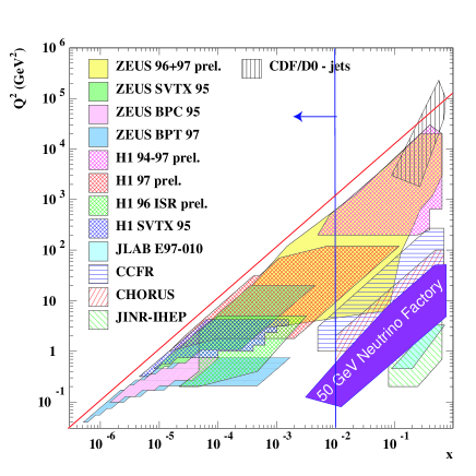
Figure 1: The kinematic plane in $x$ and $Q^{2}$ for all experiments, probing the parton distribution of the proton. The region of interest in this talk is indicated to the left of the vertical line. The other line at close to 45^o indicates the approximate kinematic limit at HERA

This increase in kinematic range has opened up a new branch of studies, which can be described generically as ‘low-$x$ physics’. As will be seen in this talk, the study of this kinematic region, which for convenience will be defined by $x<10^{-2}$, is full of interest and has already led to many advances in the understanding of the theory of the strong interaction, Quantum Chromodynamics (QCD).

Although the study of diffractive processes is intimately linked to many aspects of low-$x$ physics, constaints of time mean that it is not covered in this talk. The contribution by J. Dainton [4] to this meeting touches upon diffraction to some degree.

1.1 Theoretical background

The interest in low-$x$ physics is that particles with small $x$ are the result of a large number of QCD branching processes. The behaviour of partons at low $x$ thus reflects the dynamics of QCD and allows the behaviour of its couplings and interactions to be probed over a large range in the kinematic variables. In particular, the evolution of the number of partons as a function of $x$ and $Q^{2}$ will be sensitive, depending on the kinematic range, to the various approximations that describe QCD evolution.

Several of the contributions to this meeting have discussed the subject of QCD evolution in some depth [5, 6], and there are of course many excellent overviews of the subject [7], so that is appropriate here only to give a very brief summary of the most important points relevant at low $x$.

One of the most important properties of QCD, without which its usefulness as a theory would be extremely limited, is that of factorisation. This states that hard processes can be regarded as a convolution of a ‘sub-process’ cross section that can be calculated in terms of point-like interactions together with the probability to find the participating particles in the target and in the probe. The subsequent hadronisation of the participants in the hard collision, together with the target and probe remnants, can be regarded as an approximately independent process. Thus the cross section can be written schematically as:

$$\sigma\sim f_{t}\otimes f_{p}\otimes\hat{\sigma}$$ (1)

where $\hat{\sigma}$ is the sub-process cross section and $f_{t},f_{p}$ are the parton distribution functions for the target and probe, respectively. One of the most important results of the factorisation hypothesis is that the parton distribution functions (PDFs) measured in one process can be used in the cross-section determination for a completely different process. Furthermore, QCD provides the tools by which to extrapolate from the PDFs measured at one scale to very different scales.

Specialising now to deep inelastic scattering (DIS), the PDF for the highly virtual photon can normally be considered to be a $\delta$ function, so that equation 1 becomes:

$$\sigma\sim f\otimes\hat{\sigma}$$ (2)

where $f$ now represents the PDF of the proton. It is conventional to assume that $f$ satisfies the schematic equation:

$$\frac{\partial f}{\partial\ln\mu^{2}}\sim\frac{\alpha_{s}(\mu^{2})}{2\pi}\cdot\left(f\otimes{\cal P}\right)$$ (3)

where $\mu$ represents the renormalisation scale and ${\cal P}$ is a ‘splitting function’ that describes the probability of a given parton splitting into two others. This equation is known as the (Dokshitzer)-Gribov-Lipatov-Altarelli-Parisi equation [8, 9, 10, 11]. There are four distinct Altarelli-Parisis (AP) splitting functions representing the 4 possible $1\rightarrow 2$ splittings and referred to as $P_{qq},P_{gq},P_{qg}$ and $P_{gg}$. The calculation of the splitting functions in perturbative QCD in equation 3 requires approximations, both in order of terms which can be taken into account as well as the most important kinematic variables. The generic form for the splitting functions can be shown to be [7]:

$$x{\cal P}(x,\alpha_{s})=\sum^{\infty}_{n=0}\left(\frac{\alpha_{s}}{2\pi}\right)^{n}\left[\sum^{n}_{m=0}A^{(n)}_{m}\left\{\ln\left(\frac{1}{x}\right)\right\}^{m}+x\overline{\cal P}^{(n)}(x)\right]$$ (4)

where $\alpha_{s}$ is the strong coupling constant, $\overline{\cal P}^{(n)}(x)$ are the $x$-finite parts of the AP splitting functions and $A^{(n)}_{m}$ are numerical coefficients that can be calculated, at least in principle, for each splitting function. The AP splitting functions sum over terms proportional to $(\alpha_{s}\ln Q^{2})^{n}$ in the perturbative expansion. Thus, for example, the term in equation 4 with $n=m=0$ when added to $\overline{\cal P}^{(0)}(x)$ corresponds to leading order in so-called Gribov-Lipatov-Altarelli-Parisi (GLAP) evolution. In some kinematic regions, and in particular at low $x$, it must become essential to sum leading terms in $\ln 1/x$ independent of the value of $\ln Q^{2}$. These terms in some sense correspond to corrections taking into account so-called Balitsky-Fadin-Kuraev-Lipatov [12, 13, 14, 15] (BFKL) evolution, which governs the evolution in $x$ at fixed $Q^{2}$. As $x$ falls, this must at some point drive parton evolution. One of the continuing themes of low-$x$ physics, as will be discussed in sections 3 and 4, is the search for experimental effects that can be unambiguously attributed to BFKL evolution.

Figure 2 shows the $\ln 1/x$ - $\ln Q^{2}$ plane at HERA, together with schematic indications of the directions in which GLAP and BFKL dominate the evolution of parton distributions.

Figure 2: Schematic diagram showing different regions of the $\ln 1/x$ and $\ln Q^{2}$ plane and the evolution equations expected to hold therein. The line marked ’saturation’ represents the boundary between GLAP evolution and evolution governed by the GLR equation. The ‘size’ of partons is also indicated in differing kinematic regions.

The third direction on the figure, labelled ‘CCFM’, refers to an approach to an integrated evolution containing both the leading GLAP and BFKL terms to equal order developed by Ciafaloni, Catani, Fiorani and Marchesini [16, 17, 18]. Also indicated on the figure are schematic indications of both the ‘size’ and density of partons in the proton in different kinematic regions. The transverse size of the partons which can be resolved by a probe with virtuality $Q^{2}$ is proportional to $1/Q$, so that the area of the partonic ‘dots’ in figure 2 falls as $Q^{2}$ rises. For particular combinations of parton size and density, the proton will eventually become ‘black’ to probes, or, equivalently, the component gluons will become so dense that they will begin to recombine. The dotted line labelled ‘Critical line - GLR’ refers to the boundary beyond which it is expected that such parton saturation effects will become important, i.e. the region in which partons become so densely crowded that interactions between them reduce the growth in parton density predicted by the linear GLAP and BFKL evolution equations. The parton evolution in this region can be described by the Gribov-Levin-Riskin [19, 20] equation, which explicitly takes into account an absorptive term in the gluon evolution equation. Naively, it can be assumed [21] that the gluons inside the proton each occupies on average a transverse area of $\pi Q^{-2}$ so that the total transverse area occupied by gluons is proportional to the number density multiplied by this area, i.e. $\pi Q^{-2}xg(x,Q^{2})$. Since, as will be discussed later, the gluon density increases quickly as $x$ falls, and the gluon ‘size’ increases as $Q^{-1}$, in the region in which both $x$ and $Q^{2}$ are small, saturation effects ought to become important. This should occur when the size occupied by the partons becomes similar to the size of the proton:

$$xg(x,Q^{2})\frac{\pi}{Q^{2}}=\pi R^{2}$$ (5)

where $R$ is the radius of the proton, ($\sim 1$ fm $\sim 5$ GeV^-1). The measured values of $xg(x,Q^{2})$ imply that saturation ought to be observable at HERA [22] at low $x$ and $Q^{2}$, although the values of $Q^{2}$ which satisfy equation 5 are sufficiently small that possible non-perturbative and higher-twist effects certainly complicate the situation. Of course, it is also possible that the assumption of homogenous gluon density is incorrect; for example, the gluon density may be larger in the close vicinity of the valence quarks, giving rise to so-called ‘hot spots’ [23], which could lead to saturation being observable at smaller distances and thereby larger $Q^{2}$. The concepts of ‘shadowing’ or saturation have been discussed now for many years [20, 24, 25, 26, 27, 28, 29, 30, 31, 32, 33, 34, 35, 36, 37, 38, 39, 40, 41, 42, 43, 44, 45, 46, 47, 48, 49, 50, 51, 52, 22]. As will be seen in section 4.4, HERA does indeed provide data of relevance to such discussions.

2 The Structure Function Data

In this section, the most recent structure function data from ZEUS and H1 are presented and discussed. After some initial definitions of kinematic variables and the structure functions relevant at low $x$, the data on $F_{2}$ are shown and indirect methods of extracting the longitudinal structure function, $F_{L}$ are discussed.

2.1 Kinematics and structure function formulae

The scattering of a lepton from a proton at sufficiently large $Q^{2}$ can be viewed as the elastic scattering of the lepton from a quark or antiquark inside the proton. As such the process can be fully described by two relativistic invariants. If the initial (final) four-momentum of the lepton is $k(k^{\prime})$, the initial four-momentum of the proton is $P$, the fraction of the proton’s momentum carried by the struck quark is $x$ and the final four-momentum of the hadronic system is $P^{\prime}$, the following invariants may be constructed:

$$s = (P+k)^{2}$$ (6)

$$Q^{2} = -q^{2}=-(k^{\prime}-k)^{2}$$ (7)

$$y = \frac{P\cdot q}{P\cdot k}$$ (8)

$$W^{2} = (P^{\prime})^{2}=(P+q)^{2}$$ (9)

Energy-momentum conservation implies that:

$$x=\frac{Q^{2}}{2P\cdot q}$$ (10)

so that, ignoring the masses of the lepton and proton:

$$y = \frac{Q^{2}}{sx}$$ (11)

$$W^{2} = Q^{2}\frac{1-x}{x}\sim\frac{Q^{2}}{x}$$ (12)

where the approximate relationship will in general be sufficiently accurate for the values of $x$ of interest in this talk. Since DIS at a given $s$ can be specified by any two of these invariants, the most convenient may be chosen, normally $x$ and $Q^{2}$.

Equation 13 shows the general form for the spin-averaged neutral current differential cross section in terms of the structure functions ${F}_{1}$, ${F}_{2}$ and ${F}_{3}$:

$$\frac{d^{2}\sigma}{dxdQ^{2}} = \frac{2\pi\alpha^{2}}{xQ^{4}}\left[2xy^{2}{F}_{1}+2(1-y){F}_{2}\right.$$ (13)

$$\;\pm \left.\{1-(1-y)^{2}\}x{F}_{3}\right]$$

where the $+$ sign in the $\pm$ term is taken for $e^{-}$ and the $-$ sign for $e^{+}$ interactions. The structure functions are products of quark distribution functions and the couplings of the current mediating the interaction. They are in general functions of the two invariants required to describe the interaction.

To leading order in the QCD-improved parton model, in which quarks are massless, have spin $\frac{1}{2}$ and in which they develop no $p_{T}$, the Callan-Gross relation [53]:

$$2xF_{1}(x) = F_{2}(x)$$ (14)

is satisfied. At the next order, $p_{T}$ must be taken into account and this relation is violated. This is usually quantified by defining a longitudinal structure function, $F_{L}$, such that $F_{L}=F_{2}-2xF_{1}$. Substituting into equation 13 gives:

$$\frac{d^{2}\sigma}{dxdQ^{2}} = \frac{2\pi\alpha^{2}}{xQ^{4}}\left[Y_{+}\cdot F_{2}(x,Q^{2})\right.$$ (15)

$$\;- \left.{y^{2}}F_{L}(x,Q^{2})+Y_{-}\cdot xF_{3}(x,Q^{2})\right]$$

where $Y_{\pm}$ are kinematic factors given by:

$$Y_{\pm}=1\pm(1-y)^{2}$$ (16)

At low $x$, in general $Q^{2}\ll M_{Z}^{2}$, $xF_{3}$ vanishes and equation 15 reduces to that for photon exchange. In the rest of this talk, electroweak effects will be neglected.

In general, the form of the structure functions beyond leading order depends on the renormalisation and factorisation scheme used. In the so-called ‘DIS’ scheme, the logarithmic singularity produced by collinear gluon emission is absorbed into the definition of the quark distribution, so that the structure functions have a particularly simple form and can be expressed to all orders as

$$F_{2}(x,Q^{2}) = \sum_{i=u,d,s,c,b}A_{i}(Q^{2})\left[xq_{i}(x,Q^{2})+x\overline{q}_{i}(x,Q^{2})\right]$$ (17)

The parton distributions $q_{i}(x,Q^{2})$ and $\overline{q}_{i}(x,Q^{2})$ refer to quarks and antiquarks of type $i$. The quantities $A_{i}(Q^{2})$ are given by the square of the electric charge of quark or antiquark $i$. However, in the $\overline{MS}$ scheme, the form of $F_{2}$ changes with order in QCD. In LO QCD it has the form:

$$F_{2}(x,Q^{2}) = \sum_{i=u,d,s,c,b}A_{i}(Q^{2})\int_{x}^{1}\frac{dy}{y}\left(\frac{x}{y}\right)\left[\left\{\delta(1-\frac{x}{y})+\frac{\alpha_{s}}{2\pi}C^{\overline{\mbox{\tiny{MS}}}}_{q}\left(\frac{x}{y}\right)\right\}\right.$$ (18)

$$\cdot \left.\left(yq_{i}(y,Q^{2})+y\overline{q}_{i}(y,Q^{2})\right)+\left\{\frac{\alpha_{s}}{2\pi}C^{\overline{\mbox{\tiny{MS}}}}_{g}\left(\frac{x}{y}\right)\right\}yg(y,Q^{2})\right]$$

where $g(x,Q^{2})$ is the gluon density in the proton, $\alpha_{s}(Q^{2})$ is the QCD running coupling constant and $C_{q}(x)$ and $C_{g}(x)$ are scheme-dependent ‘coefficient functions’.

In contrast, the longitudinal structure function contains no collinear divergence at first-order in QCD so that:

$$F_{L}(x,Q^{2}) = \frac{\alpha_{s}(Q^{2})}{2\pi}\sum_{i=u,d,s,c,b}A_{i}(Q^{2})\left\{\frac{4}{3}\int_{x}^{1}\frac{dy}{y}\left(\frac{x}{y}\right)^{2}\left[yq_{f}(y,Q^{2})+y\overline{q}_{f}(y,Q^{2})\right]\right.$$ (19)

$$+ \left.2\int_{x}^{1}\frac{dy}{y}\left(\frac{x}{y}\right)^{2}\left(1-\frac{x}{y}\right)yg(y,Q^{2})\right\}$$

independent of the factorisation scheme employed.

Taking account of radiative corrections via the term $\delta_{r}$, equation 15 becomes:

$$\frac{d^{2}\sigma}{dxdQ^{2}} = \frac{2\pi\alpha^{2}}{xQ^{4}}\cdot(1+\delta_{r})\cdot\left[Y_{+}\cdot F_{2}(x,Q^{2})-{y^{2}}F_{L}(x,Q^{2})\right]$$ (20)

A useful quantity known as the ‘reduced cross section’ can be defined from equation 20 by taking the kinematic factors to the left-hand side,i.e.:

$$\frac{xQ^{4}}{2\pi\alpha^{2}Y_{+}\cdot(1+\delta)}\frac{d^{2}\sigma}{dxdQ^{2}} = \sigma_{r}$$ (21)

$$= F_{2}(x,Q^{2})-\frac{y^{2}}{Y_{+}}F_{L}(x,Q^{2})$$

and, provided $y$ is small, $\sigma_{r}$ is to a good approximation equal to $F_{2}$.

An alternative formalism to describe DIS interactions at low $x$ in terms of total virtual photon-proton cross sections is particularly useful when discussing the low-$Q^{2}$ region and the transition to real photoproduction. The total cross section can be written as the sum of the cross sections for transversely and longitudinally polarised virtual photons:

$$\sigma^{\gamma^{*}p}_{\rm tot}(W^{2},Q^{2})\equiv\sigma_{T}+\sigma_{L}$$ (22)

where $x$ and $W$ are related using equation 12. This leads directly to expressions for $F_{2}$ and $F_{L}$ in terms of virtual photon-proton cross sections:

$$\sigma^{\gamma^{*}p}_{\rm tot}(W^{2},Q^{2})\sim F_{2} =\frac{Q^{2}}{4\pi^{2}\alpha}(\sigma_{T}+\sigma_{L})$$ (23)

$$F_{L} =\frac{Q^{2}}{4\pi^{2}\alpha}\sigma_{L}$$ (24)

2.2 The $F_{2}$ data at ‘medium’ $Q^{2}$

In this section the most recent $F_{2}$ data at ‘medium’ values of $Q^{2}$ from the two HERA experiments are discussed. The term ‘medium $Q^{2}$’ used here is essentially a definition related to the characteristics of the H1 and ZEUS detectors; the term covers the structure function measurements in which the minimum scattered electron angle (and hence the minimum $Q^{2}$) that can be measured is determined by the dimensions of the main calorimeters of the two experiments. This is in contrast to the ‘low-$Q^{2}$’ region, where, as discussed in section 2.3, the minimum $Q^{2}$ range is determined by the geometric acceptance of small, special-purpose detectors placed downstream in the electron-beam direction.

The measurement of $F_{2}$ is a very complex and painstaking effort and has been often described before [54, 55]. Since both the H1 and ZEUS detectors are sufficiently hermetic, the two invariants required to define the event kinematics fully can be reconstructed from measurements on the electron, on the hadronic final state corresponding to the struck quark, or on mixtures of the two. The optimal method depends on the kinematic region of interest and on the properties and resolutions of the detectors. The size of the radiative corrections is also very dependent on the reconstruction method employed. The basic measurements made are the angles and energies of the electron and current jet. Many methods have been used by the two experiments, of which probably the most important for the measurement of $F_{2}$ are: the Electron Method, in which the energy and the angle of the scattered electron are used; the Double Angle method [56], in which the angles of the scattered electron and the current jet are used; the $\Sigma$ method [57], which uses the current jet and electron energies and the electron angle, and the $P_{T}$ method [58], which uses the Double Angle method with the additional constraint of $p_{T}$ balance.

In order to determine $F_{2}$ the following steps are carried out. First, a sample of DIS events is selected, basically by requiring an identified electron in the detector. The kinematic variables are reconstructed using one of the methods discussed above. The data are binned in $x$ and $Q^{2}$ with bin sizes determined by detector resolution, statistics, migration in and out of the bin due to the finite resolution of the experiments, etc. Estimates of the background in each bin are made and statistically subtracted. The background in the low-$x$ region is dominated by photoproduction processes in which a fake electron is reconstructed because of confusion with hadronic debris from photoproduction interactions, which of course have a much higher cross section than DIS processes. The data are corrected for acceptance, radiative effects and migration via Monte Carlo simulation. Multiplying the corrected number of events by the appropriate kinematic factors shown in equation 20 and subtracting an estimate for $F_{L}$ gives values of $F_{2}$ and hence the quark and antiquark densities in the chosen bins. There are great gains in physics terms to be made by pushing the precision of these measurements to the limits. Since for much of the available phase space systematic effects are dominant, this requires progressively better understanding of the detectors involved and simulation of their response to parts per mille.

Figure 3

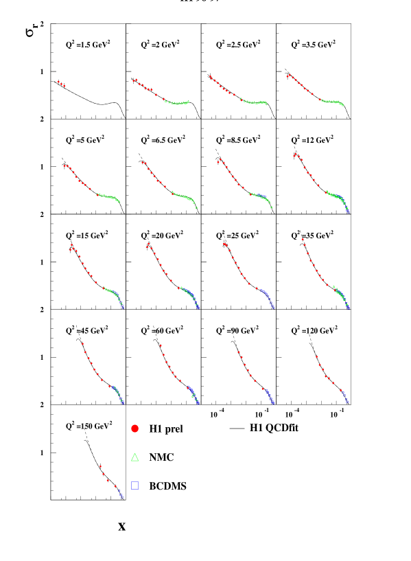
Figure 3: The preliminary H1 data on the reduced cross section (proportional to $F_{2}$) from the 1996-97 data-taking period. Also shown are points from the fixed-target experiments NMC (triangles) and BDCMS (squares). The solid curve shows the NLO QCD fit carried out by H1, while the dotted curve visible at the lowest $x$ corresponds to the expectation for $F_{L}=0$, as discussed in the text.

shows the preliminary H1 measurement of the reduced cross section (see equation 21) in bins of $Q^{2}$ as a function of $x$. Also shown are data from the fixed-target experiments NMC [59] and BCDMS [60, 61]. The bins from $Q^{2}$ = 1.5 GeV² to 150 GeV² are shown. In the relatively small region of overlap, there is good agreement between the H1 and fixed-target data. The most obvious characteristic of the data is the steep rise of $F_{2}$ at low $x$. The curve shown on the figure is the result of an NLO QCD fit by the H1 collaboration to this data together with earlier measurements at higher $x$ from NMC. The NLO QCD fit [62], based on GLAP evolution, uses three light flavours with charm added via the boson-gluon fusion process and uses $\alpha_{s}(M^{2}_{Z})=0.118$. It gives an excellent fit to the data over the full kinematic range. The quality of the QCD fit permits the conclusion that the rise of $F_{2}$ at low $x$ is unambiguously associated with a dramatic rise in the gluon distribution. Also shown in figure 3 as the dashed line is the expectation of the fit for $F_{2}$ alone. As can be seen, there is a small departure from the measured value of $\sigma_{r}$, implying that in this kinematic region, the effect of $F_{L}$ begins to become perceptible; this is discussed further in section 2.4.

Figure 4

Figure 4: The lowest $Q^{2}$ bins of the preliminary ZEUS data on $F_{2}$ from the 1996-97 data-taking period. The preliminary data are in good agreement with the published data (shown as open circles). Also shown are points from fixed-target experiments. The solid curve shows the ZEUS NLO QCD fit, while the dashed line shows the CTEQ4D curve and the dotted line that from MRST99.

shows the preliminary 1996-97 ZEUS data, plotted as the $F_{2}$ structure function as a function of $x$ in $Q^{2}$ bins with the QCD $F_{L}$ prediction subtracted. Only the lowest $Q^{2}$ bins are shown; $F_{2}$ has been determined up to $Q^{2}$ = 30,000 GeV². Fixed target data from BCDMS [60, 61], E665 [63], NMC [59], and SLAC [64] are also shown. The data agree well with the H1 data and show the same dominant feature of a very steep rise at low $x$. The data are also very well described by the NLO QCD global fit to parton distributions of CTEQ4D [65] and MRST99[66].

Figure 5 shows the H1 data together with data from NMC and BCDMS, now plotted in $x$ bins as a function of $Q^{2}$.

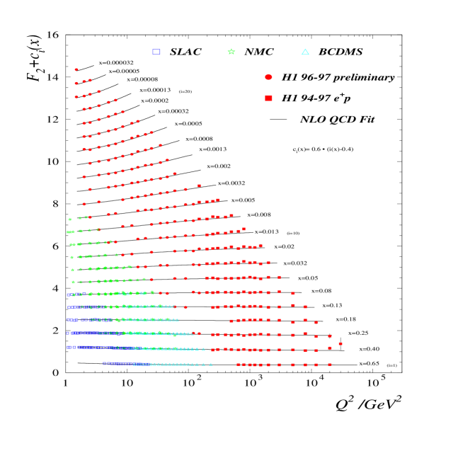
Figure 5: Preliminary H1 data on $F_{2}$ from 1996-97 and published data from 1994-97 in bins of $x$ as a function of $Q^{2}$. Also plotted are fixed-target data from SLAC, NMC and BCDMS. Each $x$ bin is offset by the amount indicated in the legend for ease of visibility. The curves show the H1 NLO QCD fit to the data. The flat ’scaling’ regime at high $x$ gives way at lower $x$ to steep scale breaking due to gluon radiation.

The data cover approximately five orders of magnitude in both $x$ and $Q^{2}$. At high $x$, approximate scaling in $Q^{2}$ can be clearly observed. As $x$ falls, deviations from scaling become stronger and stronger. The lines on the figure are the result of the NLO QCD fit, which can again be seen to give an excellent description of the data.

The H1 data for $F_{2}$ at low $x$ in $x$ bins as a function of $\ln Q^{2}$ is shown in figure 6.

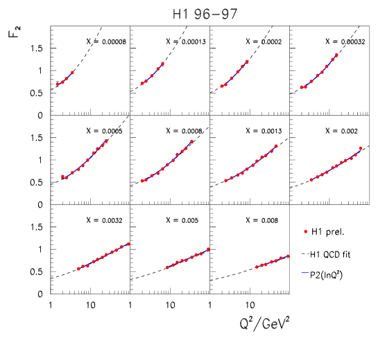
Figure 6: Preliminary H1 data on $F_{2}$ from 1996-97 in bins of $x$ as a function of $Q^{2}$. The solid line shows a fit to the form of equation 25, while the dashed line shows the H1 NLO QCD fit.

It can clearly be seen that the data are not linear in $\ln Q^{2}$. In fact they fit well to a second-order polynomial of the form

$$F_{2}=A(x)+B(x)\ln Q^{2}+C(x)(\ln Q^{2})^{2}$$ (25)

and this polynomial fit is almost indistinguishable from the H1 NLO QCD fit, except at the highest $Q^{2}$.

The most convenient and useful way to parameterise the deviations of the data from scaling is to examine the logarithmic derivative, $\partial F_{2}/\partial\ln Q^{2}$, which in leading-order QCD is directly proportional to the gluon density at twice the $x$ of the derivative:

$$\frac{\partial F_{2}}{\partial\ln Q^{2}}=\frac{2\alpha_{s}}{9\pi}xg(x,Q^{2})$$ (26)

Having fit the data to the form of equation 25, it is straight-forward to obtain the logarithmic derivative. Since this is proportional to the LO gluon density, it is clear that a precision measurement of the scaling violations can be used directly to determine the gluon distribution. Figure 7 shows such determinations from both H1 and ZEUS.

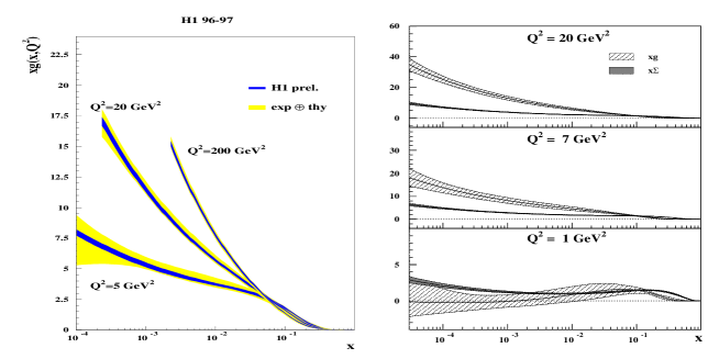
Figure 7: The left-hand plot shows preliminary H1 data on determination of the gluon from $F_{2}$ data from 1996-97. The gluon density is shown for three values of $Q^{2}$; the central band shows the statistical uncertainty while the outer bands show the systematic and the theoretical uncertainties added in quadrature. The right-hand side plot shows ZEUS data on determination of the gluon from $F_{2}$ data from 1995. The gluon density is shown for three values of $Q^{2}$; all data down to $Q^{2}>1$ GeV² is included in the NLO QCD fit. The bands show all uncertainties added in quadrature. The light shaded band is the gluon density while the dark shaded band shows the sea.

The H1 determination comes from the NLO QCD fit referred to above whereas that from ZEUS comes from an NLO fit to published data [67]. The steep rise in the gluon density as $x$ falls is apparent. Also noticeable, particularly in the ZEUS determination, is that this rise becomes weaker and weaker as $Q^{2}$ falls. Indeed, for $Q^{2}=1$ GeV², the gluon density falls below that of the singlet quark structure function and is essentially compatible with zero. This seems to contradict the ‘standard’ picture in which the rise of $F_{2}$, which is of course only directly sensitive to the density of charged partons, is driven by the quark-antiquark pairs produced from gluons. However, these interesting effects only become obvious at very low values of $Q^{2}$, and it is not clear that it makes sense to talk about ‘gluon densities’ at these low $Q^{2}$ values. Nevertheless, it is certainly true that the NLO QCD fits themselves seem to give a perfectly satisfactory description of the general features of the data down to these low values of $Q^{2}$. Much more will be said on this subject in section 4.4.

In addition to the high-precision data on the fully inclusive $F_{2}$, the ZEUS collaboration has also presented data on semi-inclusive DIS in which a charm quark or antiquark is involved in the hard scatter [68]. Figure 8

Figure 8: ZEUS data on the charm structure function, in bins of $x$ as a function of $Q^{2}$. The band shows the ZEUS NLO QCD fit.

shows the $F_{2}^{c\overline{c}}$ data in $x$ bins as a function of $Q^{2}$. A qualitatively similar pattern of scaling violations to that in the fully inclusive $F_{2}$ can be seen; however, the scaling violations seem, within the relatively large errors, to be stronger than in the inclusive case and to set in rather earlier. While part of this effect can be attributed to the effect of the charm-quark mass, it is also to be expected since the dominant process in DIS charm production is boson-gluon fusion, which is entirely driven by the gluon density in the proton. Once again, it can be seen that the NLO QCD fit gives an excellent description of the data. Figure 9

Figure 9: ZEUS data on the charm structure function, plotted as a ratio of the inclusive structure function, $F_{2}$ in bins of $Q^{2}$ as a function of $x$. The band shows the ZEUS NLO QCD fit.

shows the ratio of the charm over the inclusive $F_{2}$. At small $x$ the ratio flattens, implying that the charm and inclusive structure functions grow at the same rate, as is to be expected if both are dominated by the gluon in this region. For low values of $x$, the ratio falls at fixed $x$ as $Q^{2}$ falls. This is consistent with the observation discussed above that as $Q^{2}$ falls the gluon density at fixed $x$ also falls.

2.3 The $F_{2}$ data at ‘low’ $Q^{2}$

The ZEUS and H1 detectors are not perfectly hermetic, since it is clearly necessary to allow the beams to enter and leave the apparatus. Thus the ‘beam-hole’ limits the angular acceptance of the detectors both at very forward and very backward directions. In the very backward direction (small lepton-scattering angles) this limits the $Q^{2}$ values that can be accurately measured to around $\sim 2$ GeV². In order to access smaller $Q^{2}$ (and thereby smaller $x$), the geometrical acceptance of the detectors must be extended in some way. There are two main ways in which this has been achieved. The first is to shift the interaction vertex in the direction of the proton beam, typically by of order 60 cm, so that the electron has further to travel before it strikes the rear calorimeters. This means that the geometrical edge of the detector now corresponds to a smaller scattering angle, and hence lower $Q^{2}$ can be accepted. The other method is to install small, high precision, detectors further upstream in the electron beam direction which can thereby detect much smaller scattering angles than the main detectors. Both ZEUS and H1 have such detectors, although so far only ZEUS have published results.

ZEUS published some time ago results using their Beam Pipe Calorimeter (BPC) [69], which is a small tungsten-scintillator sampling calorimeter placed 2.94 m away from the interaction point in the electron beam direction. In 1997, two silicon-microstrip detector planes were added in front of the calorimeter in order to improve the position resolution. ZEUS has recently published the final results from this BPC/BPT combination [70], which extend the measurement of $F_{2}$ down to $x\sim 6\cdot 10^{-7}$ and $Q^{2}\sim 0.045$ GeV². Figure 10 shows the final ZEUS data in bins of $Q^{2}$ as a function of $x$.

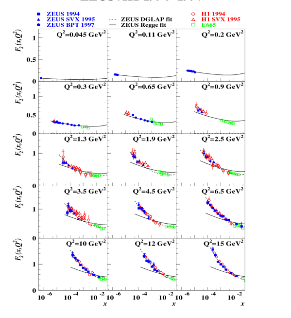
Figure 10: ZEUS BPT data on $F_{2}$ in bins of $Q^{2}$ as a function of $x$. Also shown are earlier ZEUS data as well as data from H1 and E665. The solid line shows the results of the ‘ZEUS Regge fit’ to the form of equation 27, while the dotted line shows the result of the ZEUS NLO QCD fit.

The new data match well with the previous ZEUS BPC data, as well as with that from other experiments in the overlap region. However, the extrapolation of the ZEUS Regge fit (see below) into the fixed target regime is generally of order 15% above this data.

Figure 11: ZEUS BPT data on $F_{2}$ in bins of $y$ as a function of $Q^{2}$. Also shown are earlier ZEUS data as well as data from H1 and E665. The solid line shows the results of the ‘ZEUS Regge fit’ to the form of equation 27, while the dotted line shows the result of the ZEUS NLO QCD fit.

The solid curve labelled ‘ZEUS Regge fit’ on figure 10 shows the result of a fit to the form:

$$F_{2}(x,Q^{2})=\left(\frac{Q^{2}}{4\pi^{2}\alpha}\right)\cdot\left(\frac{M_{0}^{2}}{M_{0}^{2}+Q^{2}}\right)\cdot\left(A_{\rm I\!R}\cdot\left(\frac{Q^{2}}{x}\right)^{\alpha_{\rm I\!R}-1}+A_{\rm I\!P}\cdot\left(\frac{Q^{2}}{x}\right)^{\alpha_{\rm I\!P}-1}\right)$$ (27)

where $A_{\rm I\!R},A_{\rm I\!P}$ and $M_{0}$ are constants and $\alpha_{\rm I\!R}$ and $\alpha_{\rm I\!P}$ are the Reggeon and Pomeron intercepts, respectively. This phenomenological parameterisation is based on the combination of a simplified version of the generalised vector meson dominance model [71] for the description of the $Q^{2}$ dependence and Regge theory [72] for the description of the $x$ dependence of $F_{2}$. Regge Theory is most applicable to the description of cross sections at asypmtotic energy. Equations 12 and 22, which relate $F_{2}$ to cross sections evaluated at energies proportional to $x^{-1}$, imply that Regge theory should describe the very low-$x$ data well. This is borne out by figure 10, where the ZEUS Regge fit gives a good description of the data up to $Q^{2}\sim 1$ GeV². Above this $Q^{2}$, however, the Regge description rapidly fails, whereas the ZEUS NLO QCD fit, shown for $Q^{2}>1$ GeV², is an excellent description of the data from here to the highest $Q^{2}$.

Figure 11 shows the ZEUS $F_{2}$ data in bins of constant $y$ as a function of $\ln Q^{2}$. For $Q^{2}\raisebox{-2.58334pt}{${\textstyle\stackrel{{\scriptstyle>}}{{\sim}}}$}1$ GeV², the data are roughly independent of $Q^{2}$, whereas at lower $Q^{2}$ they fall rapidly, approaching the $Q^{-2}$ fall-off that would be expected in the limit $Q^{2}\rightarrow 0$ from conservation of the electromagnetic current. Whether this dependence indicates that this limit has already been reached, or whether other effects, for instance saturation, are responsible, will be discussed in section 4.4.

2.4 The $F_{L}$ structure function

As discussed in section 2.1, the differential cross section for DIS at low $x$ depends on two structure functions, $F_{2}$ and $F_{L}$. Since in principle both $F_{2}$ and $F_{L}$ are unknown functions that depend on $x$ and $Q^{2}$, the only way in which they can be separately determined is to measure the differential cross section at fixed $x,Q^{2}$ and at different values of $y$, since as shown in equation 15, the effect of $F_{L}$ is weighted by $y^{2}$ whereas $F_{2}$ is weighted by $1+(1-y)^{2}$. However, since $Q^{2}=sxy$, fixed $x$ and $Q^{2}$ implies taking measurements at different values of $s$. This can certainly in principle be accomplished by reducing the beam energies in HERA. However, the practical difficulties for the experiments and the accelerator inherent in reducing either the proton or electron beam energy, or both, by a factor sufficient to permit an accurate measurement of $F_{L}$ mean that it has not to date been attempted. An alternative way to achieve the same end is to isolate those events in which the incoming lepton radiates a hard photon in advance of the deep inelastic scattering, thereby reducing the effective collision energy. Unfortunately, the acceptance of the luminosity taggers typically used to detect such photons is sufficiently small and understanding the acceptance sufficiently difficult that, although both experiments are working on the analysis, neither has as yet produced results.

In the absence of any direct determination, the H1 experiment has utilised its ability to detect events at very large values of $y$ in order to carry out an indirect measurement of $F_{L}$. The determinations of $F_{2}$ rely on the fact that most of the measurements are made at values of $y$ sufficiently small that the effects of $F_{L}$ are negligible; those at higher $y$ usually have an estimate of $F_{L}$, which according to QCD is in any case normally a small fraction of $F_{2}$, subtracted off. The H1 collaboration inverts this procedure by isolating kinematic regions in which the contribution of $F_{L}$ is maximised and then subtracts off the QCD prediction of $F_{2}$ measured at lower $y$.

As remarked earlier, figure 3 shows the reduced cross section, defined by equation 21, in which the contribution of $F_{L}$ can be seen at the lowest $x$ (which, for fixed $Q^{2}$, corresponds to the highest $y$) as the difference between the full QCD fit and that with $F_{L}$ set to zero. Thus, $F_{L}$ can be estimated from the following relationship:

$$F_{L}=\left(F_{2}^{\rm QCDfit}-\frac{xQ^{4}}{2\pi\alpha^{2}}\sigma_{r}\right)\cdot\frac{Y_{+}}{y^{2}}$$ (28)

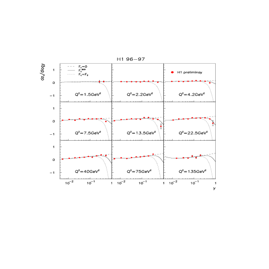
Figure 12: Preliminary H1 data on the derivative of the reduced cross section with respect to $\ln y$ in $Q^{2}$ bins. The solid curve shows the result of an NLO QCD fit with the value of $F_{L}$ as predicted by QCD from the measured $F_{2}$. The dotted line shows the same fit with $F_{L}=$ and the dashed line shows the fit with $F_{L}$ = $F_{2}$.

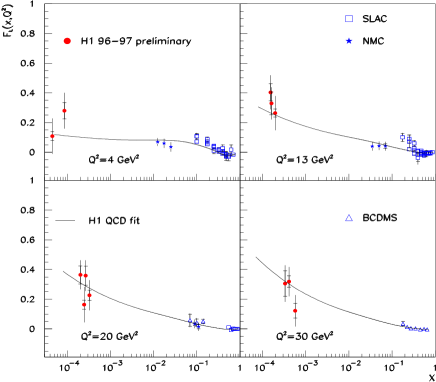
Figure 13: Preliminary H1 estimate of $F_{L}$. The $F_{L}$ values obtained are plotted in $Q^{2}$ bins as a function of $x$. Also shown are earlier bins at higher $x$ from the SLAC and NMC experiments. The solid line is the prediction of the H1 NLO QCD fit.

An alternative method used by H1 employs the derivatives of the reduced cross section with respect to $\ln y$, thereby making rather different QCD assumptions. Differentiating equation 21 leads to the following expression:

$$\frac{\partial\sigma_{r}}{\partial\ln y}=\frac{\partial F_{2}}{\partial\ln y}-\frac{2y^{2}(2-y)}{Y^{2}_{+}}F_{L}-\frac{y^{2}}{Y_{+}}\cdot\frac{\partial F_{L}}{\partial\ln y}$$ (29)

which leads to greater sensitivity to $F_{L}$ via the stronger $y$ dependence at the cost of involving derivatives of $\sigma_{r},F_{2}$ and $F_{L}$, the quantity to be measured. It is instructive to consider various restrictions:

• Small $y$ - here $\partial\sigma_{r}/\partial\ln y\sim\partial F_{2}/\partial\ln y$. For low $x$, $F_{2}$ can be well approximated by:

  $$F_{2} \propto x^{-\lambda}\propto y^{\lambda}$$ (30)

  so that:

  $$\frac{\partial F_{2}}{\partial\ln y} = \lambda y^{\lambda}$$ (31)

  which can be expanded as:

  $$\frac{\partial F_{2}}{\partial\ln y}\propto\lambda e^{\lambda\ln y}\sim\lambda(1+\lambda\ln y\ldots)$$ (32)

  provided $\lambda\ln y$ is small. From this it is clear that $\partial\sigma_{r}/\partial\ln y$ is linear in $\ln y$;

• $F_{L}=0$ - for all $y$, $\partial\sigma_{r}/\partial\ln y$ is linear in $\ln y$ for the same reason as above;

• $F_{L}\neq 0$ and large $y$ - $\partial\sigma_{r}/\partial\ln y$ is non-linear in $\ln y$ and the deviations are proportional to $F_{L}$ and its logarithmic derivative;

• $Q^{2}$ large at small $y$ - this implies $x$ becoming larger so that at some point the approximation of equation 30 starts to fail and therefore there are deviations from non-linearity.

All of these features can be seen in the preliminary H1 data of figure 12. At the largest values of $y$, the deviation from linearity implies that $F_{L}$ is non-zero. Although it is in principle possible to solve the differential equation for $F_{L}$ implied by equation 29, in practice the data are insufficiently precise, so that the value of the derivative is taken from the QCD fit. Variations in this are included in the systematic error. Also in principle it is possible to iterate the $F_{L}$ estimated in this way with that assumed in the measurement of $F_{2}$; once again, the precision of the data does not permit this and in any case the correlation would be very large.

The H1 collaboration have used the first method discussed above to estimate $F_{L}$ for $Q^{2}>10$ GeV² and the second for smaller $Q^{2}$. The results are shown in figure 13, together with earlier determinations from SLAC [64], NMC [59] and BCDMS [61]. The curve is the result of an NLO QCD fit to the H1 data deriving from the $F_{2}$ determination, i.e. by deriving the gluon and quark distributions from scaling violations and then calculating $F_{L}$ using a QCD formula such as equation 19. The QCD prediction is in good agreement with the H1 estimate.

In summary, although the indirect determinations of $F_{L}$ are both interesting and important, there is no substitute for a direct measurement. Since after the HERA upgrade the lowest $Q^{2}$ regime will no longer be accessible because of the new final-focus quadrupoles that close off the small scattering angle aperture, such data will presumably have to come from hard initial-state radiation events. First results from H1 and ZEUS are eagerly awaited.

3 Other probes of QCD dynamics at small $x$

Despite the very high precision and very large kinematic range of the structure-function data shown in the previous section, there was no obvious sign of any deviation from NLO GLAP evolution (although see section 4.4). Indeed, there are very good reasons why this should be so, even if BFKL dynamics were important [73] in this kinematic range. It is generally agreed that the chances of observing any deviation from GLAP evolution are greatly enhanced by examining certain exclusive processes in particular corners of phase space. Several such processes are examined in this section: the production of forward jets and forward $\pi^{0}$ at HERA and the study of dijets with a large separation in rapidity at the Tevatron.

3.1 Forward jet production at HERA

One of the most marked characteristics of GLAP evolution is that successive parton branchings are strongly ordered in $k_{T}^{2}$, the square of the transverse momentum of the parton. In the case of BFKL, there is essentially a random walk in $k_{T}^{2}$, while strong ordering occurs in $1/x$. These observations immediately imply the corner of phase space that is most likely to exhibit BFKL effects: small x, since this will enhance the importance of the $\ln(1/x)$ terms in the pQCD expansion, and $p_{T}$ of the struck quark $\sim Q^{2}$, which will strongly suppress GLAP evolution because of the strong $k_{T}$ ordering of successive parton branchings between the virtual photon and the struck quark [74, 75]. The kinematic properties of the struck quark can be reconstructed in several ways, of which the most usual is to tag a high-energy jet. The kinematic requirements discussed above imply selecting events with low $x$ and therefore low $Q^{2}$, so that the balancing jet with comparable $p_{T}$ will be in the very forward direction.

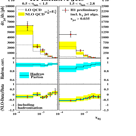
Figure 14: Preliminary H1 data on production of inclusive jets, found with the inclusive $k_{T}$ jet algorithm, in two bins of $\eta$ as a function of $x$. The dotted line shows the result of an LO QCD fit, whereas the dotted line within the shaded band shows the NLO QCD fit at a scale of $\mu_{R}^{2}=E_{T}^{2}$ with an estimate of the theoretical uncertainty. The central plots show the effect of hadronisation corrections, while the difference of the data from the NLO predictions is shown at the bottom.

The H1 collaboration presented preliminary results on forward jet production at the DIS2000 conference in Liverpool [76], in which they isolated jets using the inclusive $k_{T}$ jet algorithm in two pseudorapidity regions: ‘central’, defined as $0.5<\eta<1.5$, and ‘forward’, defined as $1.5<\eta<2.8$. Jets were selected with fractional energy $x_{\rm jet}=\frac{E_{\rm jet}}{E_{\rm pbeam}}>0.035$. The differential cross-section $d\sigma_{\rm jet}/dx$ for the ‘forward’ and ‘central’ regions is shown in figure 14. Whereas NLO QCD gives a reasonable description of the data in the central region, it clearly falls below the data in the forward region at the lowest values of $x$. Although the hadronisation corrections are largest in the forward direction, they are insufficient to explain the discrepancy. The variation in the NLO QCD prediction by varying the scale by a factor of two in each direction is also large, but again insufficient to explain the shortfall. However, $E_{T}^{2}$ is used as the hard scale in these calculations, and it is entirely unclear whether this, or $Q^{2}$, is the appropriate scale. Figure 15

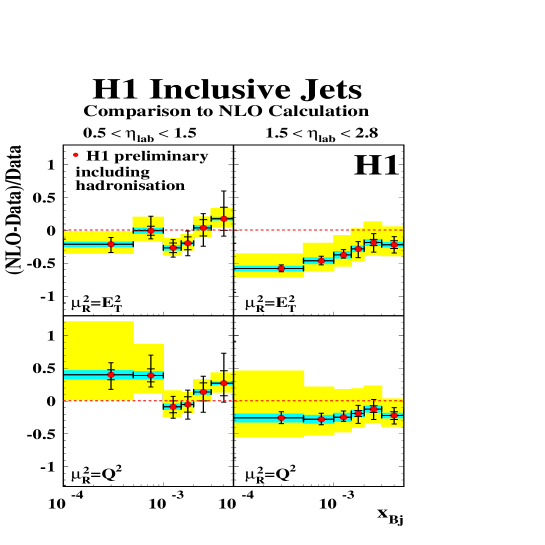
Figure 15: Preliminary H1 data on production of inclusive jets, found with the inclusive $k_{T}$ jet algorithm, in two bins of $\eta$ as a function of $x$. The plots show the difference between the data and the NLO QCD prediction. Two predictions are compared, one with a normalisation scale $\mu_{R}^{2}=E_{T}^{2}$, the other with $\mu_{R}^{2}=Q^{2}$. The central bands show the effect of hadronisation corrections, while the remaining theoretical uncertainty is shown as the outer band.

shows a comparison of the calculations assuming $E_{T}^{2}$ and $Q^{2}$ to give the hard scale in the NLO calculation. It can be seen that not only is the discrepancy reduced when $Q^{2}$ is used, the uncertainty in varying the scale from $Q^{2}/2$ to $2Q^{2}$ is sufficient to give agreement with the data. Given this theoretical uncertainty, it is clear that no firm conclusion can be drawn on the presence of non-GLAP evolution in forward jet production.

3.2 Forward $\pi^{0}$ production at HERA

Since the size of any BFKL effect will certainly strongly increase as $x$ falls, processes that can reach lower values of $x$ than possible for forward jets could be very valuable. In addition, the use of a single forward-going particle as a probe reduces the uncertainty due to jet finding algorithms as well as lowering the minimum angle which can be probed, since single particle shower profiles are significantly narrower than comparable energy jets. Such considerations led the H1 Collaboration to investigate the production of forward $\pi^{0}$s. The use of very energetic $\pi$s permits the correspondence between leading particles and the struck parton to be used to isolate a region in which BFKL effects could be important. In principle any particle species could be used; however, the power of the central tracking systems used in the HERA detectors is weakest in this region and the calorimetry in general permits both a reasonable identification of $\pi^{0}$s as well as sensitivity to smaller angles.

The H1 collaboration has isolated [77] a $\pi^{0}$ signal from 5.8 pb^-1 of data taken in 1996. The $\pi^{0}$ candidates were required to have a transverse momentum in the hadronic CMS of greater than 2.5 GeV and a $Q^{2}$ range $2<Q^{2}<70$ GeV². They were isolated between polar angles of $5^{\circ}$ and $25^{\circ}$ and required to have energy $x_{\pi}>0.01\cdot E_{p}$, where $E_{p}$ is the proton beam energy of 820 GeV. At such high energies, the two photons from the $\pi^{0}$ decay cannot be separated. Instead, they are identified by a detailed analysis of the longitudinal and transverse shape of the energy depositions in order to separate electromagnetic from hadronic showers. About 600 $\pi^{0}$ candidates were found with $p_{T}>3.5$ GeV. The efficiency for detection was around 45%.

Figure 16 shows the differential cross-section $d\sigma/dx$ for $p_{T}(\pi^{0})>3.5$ GeV.

Figure 16: The differential cross section as a function of $x$ for forward $\pi^{0}$s from the H1 Collaboration for $2<Q^{2}<70$ GeV ². The $\pi^{0}$s were required to have $p_{T}>3.5$ GeV in the hadronic centre-of-mass system, $x_{\pi}>0.01$ and angle with respect to the proton direction between $5^{o}$ and $25^{o}$. The dashed line shows the prediction from RAPGAP and the dotted line that from LEPTO. The solid line shows the result of a modified LO BFKL calculation (see text).

Also shown are predictions from the RAPGAP and LEPTO Monte Carlo programs, as well as the prediction from a modified LO BFKL calculation [78] convoluted with $\pi^{0}$ fragmentation functions. The LEPTO model [79] does not give a good description of the data. A considerable improvement is given by a model, RAPGAP2.06 [80], which includes resolved virtual photons in the hard scattering process. Such resolved processes have been shown to be important in DIS in some kinematic regions [81] even at moderate $Q^{2}$. Nevertheless, even taking into account the uncertainty caused by varying the renormalisation scale, RAPGAP cannot fit the data over the full kinematic range. However, the ARIADNE model, which is not shown in the figure, can give a good description of the data, although there is considerable arbitrariness in its predictions. The LO BFKL parton calculation is in good agreement with the data. However, once again there is a large uncertainty caused by a variation in the renormalisation scale of a factor two above and below the nominal value, leading to a 60% variation in the prediction.

Although the agreement of the BFKL model with the data is interesting, overall the inherent uncertainties in the various models are such that it is difficult to draw any clear conclusion as to the presence of BFKL effects in the data.

3.3 BFKL tests at the Tevatron

The Tevatron gives access to a rather different kinematic range in which BFKL effects could possibly become important. Here, in the production of high-energy jets, the centre-of-mass energy can be much larger than the momentum transfer, $Q$, so that the jet cross section contains large logarithms, $\ln(s/Q^{2})$, which must be summed to all orders. Such a summation can be achieved using the BFKL formalism. The D0 Collaboration[82] has isolated dijet events with very large rapidity separations and measured the cross section as a function of $x_{1}$, $x_{2}$ and $Q^{2}$, where 1 and 2 label the most-forward and most-backward jets, respectively. The longitudinal momentum fractions of the proton and antiproton, $x_{1}$ and $x_{2}$, carried by the two interacting partons are defined as:

$$x_{1,2}=\frac{2E_{T_{1,2}}}{\sqrt{s}}\;e^{\pm\overline{\eta}}\;\cosh(\Delta\eta/2)\;$$ (33)

where $E_{T_{1}}(E_{T_{2}})$ and $\eta_{1}(\eta_{2}$) are the transverse energy and pseudorapidity of the most forward(backward) jet, $\Delta\eta=\eta_{1}-\eta_{2}\geq 0$, and $\overline{\eta}=(\eta_{1}+\eta_{2})/2$. Thus, by measuring the cross section at the largest accessible values of $\Delta\eta$, the separation in $x$ of the colliding partons is maximised, thereby optimising the phase space for gluon ladders with strong ordering in $x$, i.e. BFKL evolution, to be produced. The momentum transfer during the hard scattering is defined as:

$$Q=\sqrt{E_{T_{1}}E_{T_{2}}}$$

The BFKL prediction [83] for the cross section is:

$$\hat{\sigma}_{\rm BFKL}\propto\frac{1}{Q^{2}}\cdot\frac{e^{(\alpha_{BFKL}-1)\Delta\eta}}{\sqrt{\alpha_{s}\Delta\eta}}\;$$ (34)

where $\alpha_{BFKL}$ is the BFKL intercept that governs the strength of the growth of the gluon distribution at small $x$, which in leading logarithmic approximation (LLA), is given by:

$$\alpha_{BFKL}-1=\frac{\alpha_{S}(Q)\,12\ln 2}{\pi}$$ (35)

Figure 17: The ratio of jet cross sections with rapidity gaps between them measured at $\surd s=$ 1800 and 630 GeV by the D0 Collaboration. The data points are plotted as filled circles for rapidity gaps greater than 1, and 2, as a function of the mean rapidity gap at 630 GeV. The light shaded circles represent the predictions from HERWIG while the square represents a calculation based on the LLA BFKL approach. The thick error bars denote the statistical uncertainty, while the thin error bar denotes the statistic and systematic uncertainties added in quadrature.

The cross section is a convolution of the probability to find the interacting partons with given values of $x$ inside the proton, together with the partonic scattering cross sections that contain the BFKL effects of interest. In order to remove the dependence of the cross section on the parton distribution functions, it is convenient to measure the cross sections at different centre-of-mass energy and take the ratio at fixed $x_{1},x_{2}$ and $Q^{2}$; this also reduces some correlated systematic effects stemming from the detector characteristics. The ratio of cross sections can be obtained from equation 34:

$$R\equiv\frac{\sigma(\sqrt{s_{A}})}{\sigma(\sqrt{s_{B}})}=\frac{\hat{\sigma}(\Delta\eta_{A})}{\hat{\sigma}(\Delta\eta_{B})}=\frac{e^{(\alpha_{BFKL}-1)(\Delta\eta_{A}-\Delta\eta_{B})}}{\sqrt{\Delta\eta_{A}/\Delta\eta_{B}}}$$ (36)

Clearly, the greater the difference between the two centre-of-mass energies, the greater the effective variation in $\Delta\eta$ between the two data sets and thereby the larger the BFKL effects should become.

The data samples used in the D0 analysis was taken at $\surd s=$ 1800 and 630 GeV. The $x_{1},x_{2}$ ranges were restricted to lie between 0.06 and 0.22 in order to avoid detector biases. Only one $Q^{2}$ bin was used, with $400<Q^{2}<1000$ GeV². Figure 17 shows the ratio of the cross sections at the two centre-of-mass energies as a function of the mean separation in $\eta$ in the 630 GeV data set. Also shown on the plot are the predictions from LO GLAP evolution, from the HERWIG Monte Carlo, and from the BFKL calculation. The data agree with none of the models, showing a much steeper increase than predicted even by the BFKL calculation. However, the steep rise is certainly more in accord with the BFKL prediction than that of LO GLAP evolution; what the rise in the HERWIG predictions means is unclear, at least to this author. In conclusion, the situation is yet again confused.

To summarise this section, despite having examined specific exclusive processes in which the effects of BFKL evolution are expected to be maximal, the current experimental situation is that there is little firmer evidence for deviations from standard GLAP evolution than there was in the inclusive $F_{2}$ data.

4 Interpretation and Models

While the standard perturbative QCD GLAP evolution reigns supreme at medium $x$ and high $Q^{2}$, the area of low $x$ is a particularly rich and complex area in which this perturbative QCD anzatz meets and competes with a large variety of other approaches, some based on QCD, others either on older paradigms such as Regge theory or essentially ad-hoc phenomenological models. In this section a far-from-exhaustive survey of such models is undertaken. Often it is convenient to concentrate on a particular model in order to confront specific predictions with the data. This in no way necessarily implies that such an example model is the best one available, or that others can be ignored in its favour - rather it is an attempt to illustrate generic characteristics of particular classes of approach to the elucidation of the data.

In this section the older, Regge-based approach to the understanding of $F_{2}$ is examined, followed by models that give simple parameterizations of the structure functions based, more or less loosely, on pQCD. A brief overview of the current state of global fits to the parton distribution functions is then carried out, followed by a discussion of new data from ZEUS on the logarithmic derivatives of $F_{2}$ and possible implications for QCD evolution. Dipole models, in particular that of Golec-Biernat & Wüsthoff [84, 85] are discussed in some detail and compared to the data.

4.1 Regge-based models of $F_{2}$

Regge theory [86, 87, 72] has a long and distinguished history in particle physics as a conceptual basis linking bound-state spectra, forces between particles and the cross-section behaviour as a function of energy over a wide variety of processes through the analytical properties of high-energy scattering amplitudes. The basis of the theory is that solutions of the Schrödinger equation for non-relativistic potential scattering can be solved in terms of a complex angular momentum variable, $j$. For many potentials, the only singularities of the scattering amplitude are poles in the complex angular momentum plane, known as ’Regge poles’. Somewhat surprisingly, such non-relativistic concepts have proven to be very useful in particle physics. To take the specific example relevant to this discussion, any total cross section having a power-law dependence on the centre-of-mass energy lends itself to a simple explanation in terms of Regge poles corresponding to the exchange of specific particles. The most important poles are those corresponding to the exchange of vector and tensor mesons, which give a pole at $j$ = 1/2, and that near to $j=1$, which corresponds to a particle with the quantum numbers of the vacuum that has never been observed as a final-state particle. This particle is known as the Pomeron, and is thought of as the exchanged particle that mediates elastic and diffractive scattering. In fact, if the pole is assumed to be at $j=1.08$, known as the ‘soft Pomeron’ singularity, then it gives a good description of the cross sections of a wide variety of hadronic processes [88].

The advent of HERA, allowing access to large $W^{2}$ in both soft and hard processes, offered a fertile ground for the application of Regge theory, since it works par excellence at very high energies; for example, in DIS when $W^{2}$ is much greater than any other invariant. Indeed, equations 12 and  23 make it clear that, at low $x$, $F_{2}$ can be expressed in terms of high-energy transverse and longitudinal cross sections. It was therefore interesting to discover that the strong rise in $F_{2}$ at low $x$ discovered at HERA, which can be parameterised as $x^{-\lambda}\sim W^{\lambda}$, was incompatible with the soft Pomeron intercept that had worked so well in many other reactions. Donnachie and Landshoff [89] suggested that a good description could be achieved if a further simple Regge pole were assumed at $j=1.435$, the so-called ‘hard Pomeron’. They fit to the form:

$$F_{2}(x,Q^{2})=\sum_{i=0}^{3}f_{i}(Q^{2})x^{-\epsilon_{i}}$$ (37)

and, as can be seen from figure 18, such an ansatz does indeed give a good description of the $F_{2}$ data at low $x$ (and indeed at higher $x$ as well).

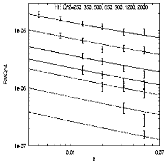
Figure 18: The H1 published data on $F_{2}$ plotted divided by $Q^{4}$ in different $Q^{2}$ bins as a function of $x$. The lines show Donnachie and Landshoff’s fits using Reggeon, soft and hard Pomeron contributions.

Donnachie and Landshoff also looked at the ZEUS data on the charm structure function, $F_{2}^{c\overline{c}}$ [90]. Here, presumably because the mass of the charm quark provides a hard scale, there is no requirement for the vector and tensor meson or the ‘soft Pomeron’ pole, leaving only one term in equation 37. The fit shown in figure 19 to the ‘hard Pomeron’ term only gives a good fit to the data.

Figure 19: ZEUS data on $F_{2}^{c\overline{c}}$ plotted divided by $Q^{4}$ as a function of $x$. The lines show the Donnachie-Landshoff prediction with only the hard Pomeron term in the fit.

Despite the successes of this approach, there are several major drawbacks. Firstly, the $f_{i}(Q^{2})$ in equation 37 cannot be predicted from Regge theory. Having added one extra Pomeron, there is no logical reason not to add others when HERA data from other channels [91, 92, 93] and improved accuracy imply deviations from a ‘universal’ two-Pomeron ansatz. Indeed, more complex singularities than poles can also be added [94, 95, 96] leading to behaviour more complex than simple powers of $W$. Thus, the Regge description can have many essentially arbitrary parameters and risks becoming merely a phenomenological parameterisation. The great range of seemingly disparate phenomena that can be explained in the Regge framework nevertheless implies that any more comprehensive theory of the strong interaction, viz. QCD, must somehow ‘explain’ or assimilate Regge concepts in a natural way. This line of investigation is a fruitful one currently being actively pursued and also leads naturally into the next section.

4.2 QCD-inspired parameterisations

The double-logarithmic limit of QCD, in which both $Q^{2}$ and $1/x$ become very large, has long been known to imply [97] that $F_{2}$ should fit to the form:

$$F_{2}(x,Q^{2})\propto\exp{\{\sqrt{(48/\beta_{0})\ln(1/x)\ln\ln Q^{2}}\}}$$ (38)

where $\beta_{0}$ is the standard Renormalisation Group Equation $\beta$ function. Ball and Forte [98, 99] showed that indeed the HERA data were well represented by this form, which they refer to as ‘double-asymptotic scaling’.

Other authors have examined functional forms that are related to the double-asymptotic scaling of equation 38. Buchmüller and Haidt [100] set out the theoretical region of validity of the so-called ‘double-logarithmic’ scaling regime. The functional form is:

$$F_{2}(x,Q^{2})=m\ln\left(\frac{Q^{2}+Q_{0}^{2}}{Q_{0}^{2}}\right)\ln\left(\frac{x_{0}}{x}\right)=m\xi$$ (39)

where $m$ is a constant to be determined from the data. Figure 20 shows [103] HERA data plotted as a function of $\xi$ to this functional form.

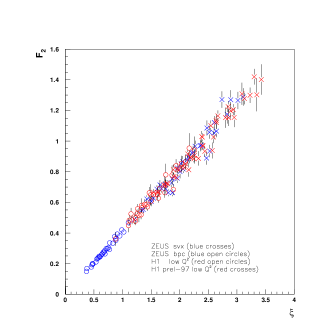
Figure 20: ZEUS and H1 $F_{2}$ data plotted against the scaling variable $\xi$ (see equation 39).

A linear fit [103] is remarkably good. This functional form is appropriate to the Regge limit of fixed $Q^{2}$ and $x\rightarrow 0$, and indeed it corresponds to the first term of the more general solution to the double-asymptotic form viz. a summation of all terms of the form [100]

$$\left(\alpha_{s}\ln\frac{Q^{2}}{\Lambda^{2}}\ln\frac{1}{x}\right)^{n}$$ (40)

which rises faster than any power of $\ln 1/x$ as $x$ falls. In the more general case in which both $Q^{2}$ and $1/x$ become large, or at sufficiently small $x$, the double-asymptotic form ought to become more appropriate. In fact, somewhat surprisingly, it would seem that even at very small $x$ the double-logarithmic form gives a good fit to the data.

A parameterisation clearly related to both the double-asymptotic and double-logarithmic ones has recently been used by Erdmann [104], in particular to facilitate comparison between the proton, photon and Pomeron structure functions. It has the form:

$$F_{2}(x,Q^{2})=a(x)\left[\ln\left(\frac{Q^{2}}{\Lambda^{2}}\right)\right]^{\kappa(x)}$$ (41)

where $\Lambda$ is the QCD scale parameter. Figure 21 shows that this form gives a good fit to the preliminary H1 $F_{2}$ data.

Figure 21: Preliminary H1 $F_{2}$ data fit to the form of equation 41.

It is also true for the published ZEUS and the BCDMS data, even at high $x$. In some sense equation 41 represents the alternative approximation to the Regge limit of Haidt, i.e. fixed $x$ and $Q^{2}$ large. The fact that both $a$ and $\kappa$ are functions of $x$ however allows the $\ln 1/x$-like terms in the sum of equation 40 to be approximately taken into account, so that the parameterisation also works well at low $Q^{2}$ and $x$. It can be seen by comparison with equation 18 that $a(x)$ is proportional to the charged parton distribution at a particular value of $Q^{2}$, viz. that for which $\ln Q^{2}/\Lambda^{2}$ = 1, and that $\kappa$ is related to the scale-breaking of $F_{2}$ and therefore to gluon radiation from the partons.

Figure 22 shows the values of $a$ and $\kappa$ as a function of $x$. The valence quark distribution at high $x$ can be very clearly seen, as well as that fact that for the low-$x$ regime of interest here, $a(x)$ is approximately constant. This implies that the scale-breaking represented by $\kappa$ is what drives the increase in $F_{2}$. Figure 22 shows that $\kappa$ increases more or less linearly from the negative scale-breaking at high $x$ until at least $x\raisebox{-2.58334pt}{${\textstyle\stackrel{{\scriptstyle>}}{{\sim}}}$}10^{-4}$, at which point it seems to level off. The implications of this observation will be discussed in more detail in section 4.4 in conjunction with the ZEUS data at very low $x$.

Figure 22: The values of the coefficients in equation 41 as a function of $x$ after fits of this functional form to BCDMS, H1 and ZEUS $F_{2}$ data (filled symbols). The open symbols correspond to photoproduction and diffractive data that are not discussed in the text.

4.3 Global fits

The extension of the kinematic range and the high-precision data on $F_{2}$ from HERA provided a substantial impetus to the determination of parton distribution functions via global fits to a wide variety of data. The major approaches are due to the CTEQ group [105], Glück, Reya and Vogt (GRV) [106] and Martin et al. (MRST) [107]. In general all groups fit to data from fixed target muon and neutrino deep inelastic scattering data, the HERA DIS data from HERMES, H1 and ZEUS, the $W$-asymmetry data from the Tevatron as well as to selected process varying from group to group such as prompt photon data from Fermilab as well as high-$E_{T}$ jet production at the Tevatron. The different data sets give different sensitivity to the proton distributions depending on the kinematic range, but together constrain them across almost the whole kinematic plane, with the possible exception of the very largest values of $x$, where significant uncertainties still remain [108].

The approach of GRV is somewhat different from that of the other two groups. They utilise the fact that, as $Q^{2}$ $\rightarrow 0$, parton distributions are fully constrained by the charge and momentum sum rules. By assuming valence-like distributions for the quarks at a very low starting $Q^{2}$, in principle the gluon and sea distributions can be generated purely dynamically. However, it is found that such a procedure generates parton distributions which are too steep as $x$ decreases. Instead they input ‘valence-like’ distributions for both quarks and gluons fixed by high-$x$ data at a larger though still very small $Q^{2}$. The starting value, $Q^{2}_{0}$, is determined by the point at which the input gluon distribution is of the same order as the input $u$ valence quark distribution and is $\sim 0.5$ GeV² in NLO QCD [109]. Although there are quite large uncertainties on the value of $Q^{2}_{0}$ and on the valence-like distributions assumed at $Q^{2}_{0}$, the effect of these is suppressed in the comparison with the high-$Q^{2}$ HERA data by the long evolution distance. In general, the GRV parameterisation gives good fits to the HERA data, as shown in figure 23, although as $Q^{2}\rightarrow Q^{2}_{0}$ the fit becomes worse, as would be expected from the formalism. In addition, however, GRV at NLO has difficulties in fitting the logarithmic derivatives of $F_{2}$ for values of $x<10^{-3}$ [110] (although see section 4.4).

Figure 23: The GRV98 fit to the ZEUS and H1 $F_{2}$ data in the low-$Q^{2}$ region in bins of $Q^{2}$ plotted as a function of $x$.

The approaches of CTEQ and MRST are basically similar, although they differ both in the data sets used as well as in the fitting procedure and the technical details of the theoretical tools used, e.g. the treatment of heavy quarks in DIS. In their latest fits CTEQ prefer to omit the prompt photon data because of the uncertainties in scale dependence and the appropriate value for the intrinsic $k_{T}$ required to fit the data. Instead they use single-jet inclusive $E_{T}$ distributions to constrain the gluon distribution at large $x$. In contrast, until their most recent publication, MRST retained the prompt photon data, giving alternative PDFs depending on the value for the prompt-photon intrinsic $k_{T}$ used. Both groups parameterise the parton distributions in terms of powers of $x$ and $(1-x)$ leading to fits with many free parameters. The MRST NLO parameterisation of the gluon is shown below as an example:

$$xg = A_{g}x^{-\lambda_{g}}(1-x)^{\eta_{g}}(1+\epsilon_{g}\sqrt{x}+\gamma_{g}x)$$ (42)

where $A_{g},\lambda_{g},\eta_{g},\epsilon_{g}$ and $\gamma_{g}$ are free parameters in the fit. The treatment of the $d/u$ ratio at high $x$ has recently been addressed by Yang and Bodek [108], who point out that deuterium binding corrections should be applied to the NMC $F_{2}^{n}/F_{2}^{p}$ data. Such corrections give good fits in the global analyses, except to the uncorrected NMC data themselves. The PDFs determined from the CTEQ5M fit are shown in figure 24 at $Q^{2}=$ 25 GeV². The steep rise of the gluon and sea distributions as $x$ falls is evident.

Figure 24: The PDFs resulting from the CTEQ5M fits at $Q^{2}$ = 25 GeV².

A long-standing problem with the various global PDFs has been the fact that no error was associated with the central values. The difficulties associated with producing such errors from a multi-parameter fit to many data sets with differing correlations are certainly formidable. It is therefore an extremely important and welcome development that Botje has recently produced for the first time PDFs with associated error matrices [111]. Figure 25 shows the valence- and sea-quark distributions together with that of the gluon from Botje’s analysis.

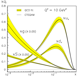
Figure 25: The valence quark, sea quark and gluon PDFs resulting from the Botje fit. The bands show the uncertainty associated with each PDF.

The fit utilises a more restricted range of data than the CTEQ and MRST fits, using the H1 and ZEUS $F_{2}$ data together with the fixed target muon and neutrino data; the Drell-Yan data from E866 [112] are used to constrain the $\overline{u}-\overline{d}$ distribution. Despite the more restricted data sets used, the results of the fit are very compatible with the most recent fits of CTEQ and MRST. The importance of the error matrices produced by this fit can be illustrated by the example shown in figure 26.

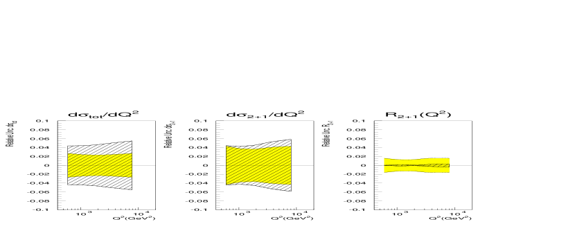
Figure 26: The uncertainty of three quantities used in the ZEUS determination of $\alpha_{s}$ from dijets in DIS. The cross section differential in $Q^{2}$, the dijet differential cross section, and the ratio of the dijet to the total cross section are shown. The shaded area shows the effect of taking the correlated errors produced by the Botje fit properly into account, the hatched area that of ignoring the correlations.

Here the effect of the errors on the uncertainty in the prediction of various cross sections and ratios in the ZEUS DIS dijet analysis [113] is shown. The very large difference in the estimated error, depending on whether the correlations between the parameters in the PDFs are taken into account of not, is striking and of the highest importance in a realistic calculation of the error on quantities such as $\alpha_{s}$.

All of the parameterisations discussed above were carried out in the framework of NLO QCD. With the increasing precision of the DIS data, as well as the need for accurate predictions of cross sections at the LHC, the need for next-to-next-to-leading-order (NNLO) fits is obvious. The first steps in this regard have already begun, and some moments of the NNLO splitting functions have already been calculated [114]. Using this with other available information, van Neerven and Vogt [115, 116] have produced analytical expressions for the splitting functions which represent the slowest and faster evolution consistent with the currently available information. The MRST group has recently used this information to investigate NNLO fits to the available data [117]. Such an analysis requires some changes to the parameterisations used, so that for example the NLO parameterisation of the gluon of equation 42 becomes:

$$xg(x,Q_{0}^{2})\;=\;A_{g}\>x^{-\lambda_{g}}\>(1-x)^{\eta_{g}}\>(1+\varepsilon_{g}\sqrt{x}+\gamma_{g}x)\>-\>A_{g}^{\prime}\>x^{-\lambda_{g}^{\prime}}\>(1-x)^{\eta_{g}^{\prime}}$$ (43)

primarily in order to facilitate a negative gluon density at low $x$ and low $Q^{2}$, which, although conceptually somewhat bizarre, is nevertheless preferred by the fits, even at NLO. The results of the ‘central’ fit, between the extremes of the van Neerven-Vogt parameterisation, is shown in figure 27.

Figure 27: The MRST ‘central’ NNLO fit to DIS data. The solid line shows the NNLO fit, while the NLO fit is shown by the dashed line and the LO fit by the dotted line. The data are from H1, ZEUS and the fixed target experiments and are plotted in $x$ bins as a function of $Q^{2}$ with an additive constant added to the data of each $x$ bin to improve visibility.

There are also changes of the LO and NLO fits with respect to earlier publications, in as much as MRST now follow CTEQ in using the Tevatron high-$E_{T}$ data rather than the prompt-photon data, and preliminary HERA $F_{2}$ data has been included in the fit. There is a marked improvement in the quality of the fit in the progression LO $\rightarrow$ NLO $\rightarrow$ NNLO, in particular in terms of the NMC data. The size of higher-twist contributions at low $x$ also decreases, so that at NNLO is it essentially negligible. The effect of going to NNLO on the PDFs themselves is highly non-trivial. This is illustrated in figure 28, where the quite major changes in $F_{L}$, particularly at low $x$, are evident. There is also a large variation depending on the choices made in the parameter space allowed by the partial NNLO ansatz. Indeed, the GLAP approach is not convergent for $Q^{2}<5$GeV², which may well be due to the neglect of important $\ln 1/x$ contributions. However, the instability seen at low $Q^{2}$ soon vanishes at higher $Q^{2}$.

Figure 28: The $F_{L}$ structure function from the MRST fits, taking into account part of the NNLO corrections in four bins of $Q^{2}$ as a function of $x$. The solid line shows the ’average’ of the parameter space available to choose the NNLO parameters, while the dashed-dotted lines show the two extreme possibilities. The NLO fit is indicated by the dashed line while the LO fit is indicated by the dotted line.

Thorne has indeed investigated the question of incorporating $\ln 1/x$ terms in the splitting functions by incorporating the solution of the NLO BFKL kernel using a running coupling constant [118, *misc:DIS2000:Thorne]. The results are shown in figure 29.

Figure 29: The NNLO MRST fit, modified by Thorne to include a NLO BFKL kernel. The ‘standard’ NNLO fit is shown as the full line, the dashed line shows the NLO fit and the dotted line the Thorne BFKL modification.

It is clear that the inclusion of the BFKL terms does indeed give an improved fit compared to the ‘central’ NNLO fit, particularly at the lowest $Q^{2}$ and $x$. This may be one of the first unambiguous indications of the importance of BFKL evolution; if so, it is rather surprising that it has occurred in the analysis of the inclusive data, rather than the exclusive channels, expected to be more sensitive, that were examined in section 3.

In conclusion, there have been major advances in the field of parton distribution functions and global fits in the last year. Not only is there now a parameterisation which gives produces associated error matrices, which is of first importance in the treatment and extraction of experimental results, but also the first attempts to incorporate NNLO corrections into the fitting has begun. In the latter case, it is clear that there is still a great deal of work required before there is a real understanding of the effects of a full NNLO treatment; not the least of the work is in the onerous task of deriving all the necessary NNLO terms. It may still be premature [120] to worry too much about the somewhat strange behaviour of the NNLO gluon density and $F_{L}$, until a full NNLO treatment is possible. Nevertheless, the increased precision of the data becoming available and the rapid theoretical developments combine to make the subject of global PDF fitting and structure functions both topical and interesting.

4.4 $F_{2}$ and its derivatives

With the publication of the final data from the very low-$(Q^{2},x)$ region measured with the Beam Pipe Tracker (BPT) [70] as well as the latest high-precision $F_{2}$ data, ZEUS now has precise data over a remarkable six orders of magnitude in $x$ and $Q^{2}$. This data is shown in $x$ bins as a function of $\ln Q^{2}$ in figure 30, together with fixed target data from NMC and E665, which extends the range in the direction of medium $x$ and $Q^{2}$.

Figure 30: Compilation of ZEUS $F_{2}$ data, both published and preliminary from the 1996-97 data sample in $x$ bins as a function of $Q^{2}$. Each $x$ bin is shifted by an additive constant for ease of visibility. Data from NMC and E665 is also shown. The dotted lines show lines of constant $W$, while the solid lines are fits to the form of equation 44.

The availability of this very wide range of precise data makes possible qualitatively new investigations of models that describe $F_{2}$. As discussed in section 2.2, the logarithmic derivative of $F_{2}$ is directly proportional to the gluon density, which in turn is by far the dominant parton density at the small values of $x$ of interest here. It is therefore interesting to examine the behaviour of such logarithmic derivatives as a function of both $x$ and $Q^{2}$. Plots of $\partial F_{2}/\partial\ln Q^{2}$ as a function of $x$ were first presented for the ZEUS data by Caldwell at the DESY Theory Workshop in 1997 and subsequently published by ZEUS [121], and led to much comment in the literature. The range and quality of the data available at the time meant that severe restrictions were placed on how the data could be binned and parameterised. These restrictions led to several erroneous suggestions that the features of this plot were a consequence of trivial kinematics. The quality and range of the currently available data now permits a much better-defined procedure to be followed in constructing plots of the logarithmic derivative.

The data shown in figure 30, particularly in the lower-$x$ bins, are clearly inconsistent with a linear dependence on $\ln Q^{2}$, as was pointed out for the preliminary H1 data by Klein [62]. The solid curves on the figure correspond to fits to a polynomial in $\ln Q^{2}$ of the form:

$$F_{2}=A(x)+B(x)\left(\log_{10}Q^{2}\right)+C(x)\left(\log_{10}Q^{2}\right)^{2}$$ (44)

which gives a good fit to the data through the entire kinematic range. The dotted lines on figure 30 are lines of constant $W$. The curious ‘bulging’ shape of these contours of constant $W$ in the small-$x$ region immediately implies that something interesting is going on there. Indeed, simple inspection of figure 30 shows that the slope of $F_{2}$ at constant $W$ begins flat in the scaling region, increases markedly as the gluon grows and drives the evolution of $F_{2}$ and then flattens off again at the lowest $x$.

This behaviour is made clear and explicit in figure 31, which shows the logarithmic derivative evaluated at $(x,Q^{2})$ points along the contours of fixed $W$ shown on figure 30 according to the derivative of equation 44, viz.:

$$\frac{\partial F_{2}}{\partial\log_{10}Q^{2}}=B(x)+2C(x)\log_{10}Q^{2}$$ (45)

where the data are plotted separately as functions of $\ln Q^{2}$ and $\ln x$.

Figure 31: The logarithmic derivative of the ZEUS $F_{2}$ data in six bins of $W$, plotted as a function of $Q^{2}$ and $x$.

The data was adjusted where necessary to the appropriate $Q^{2},x,W$-bin by using the ALLM parameterisation [122]. The error bars on the points are evaluated from the errors on the parameters in equation 44 and consist of the statistical and systematic uncertainties added in quadrature. The correlations on the errors are, however, not taken into account, so that the error bars shown are slight over-estimates.

The turn-over in the derivatives in all $W$ bins is marked, and confirms the similar feature seen in the original ZEUS plot, but now with much better defined kinematic conditions. When plotted as a function of $\ln Q^{2}$, the maximum in the derivative moves to larger $Q^{2}$ as $W$ increases, while as a function of $\ln x$, the maximum moves to smaller $x$ as $W$ increases.

It is of interest to speculate at this point as to what dynamical mechanism might be causing the behaviour exhibited in figure 31. Since the logarithmic derivative is proportional at leading order to the gluon density, the obvious inference that can be drawn from the data is that the rise in the gluon density at low $x$ begins to soften and eventually to fall as $x$ decreases. Indeed, several indications of such an effect have been discussed in earlier sections of this talk. Such an effect is by no means, as will be seen below, necessarily an indication of deviations from GLAP evolution. Nevertheless, such a fall in the gluon density as $x$ falls is a natural consequence of many models of parton saturation or shadowing, so that it is of interest to explore their features in more detail at this point. Before beginning however, it is important to emphasise that the relative emphasis on dipole models in this talk is not an indication that they are necessarily ‘correct’, or even necessarily give a better description of the data than other models, such as the standard twist-two QCD descriptions. Neverthless, they do have several attractive features, in particular the rather natural way in which they can lead to a unified description of diffraction and deep inelastic scattering, which makes it useful to discuss their features in some detail here; not least since in general their concepts are less familiar to the average particle physicist.

4.4.1 Dipole models and shadowing

Dipole models of DIS have a long history. The basic idea is to transform the ‘normal’ way of looking at DIS, which considers a virtual photon to be emitted from the incoming lepton and to collide with a parton emanating from the proton, by transforming to a topologically equivalent process in which the virtual photon splits into a quark-antiquark pair. These two descriptions are related by a Lorentz transform, since the ‘normal’ view of partons evolving inside the proton is appropriate to a frame such as the Breit frame or the infinite-momentum frame, whereas the dipole picture is more appropriate to the rest frame of proton. In the rest frame of the proton, the virtual photon splits into a quark-antiquark pair, or dipole, well downstream of the proton. The formation time of the dipole in the proton rest frame is related to the uncertainty in the energy of the pair by $\tau_{q\overline{q}}\sim 1/\Delta E$, which, in the limit of small $x$ becomes [123] $\tau_{q\overline{q}}\sim 1/(xM_{p})$, where $M_{p}$ is the proton rest mass. Since the distance between the formation of the dipole and the interaction with the proton implied by this lifetime is much larger than the proton radius, the transverse size of the dipole can be considered fixed during the interaction. Thus, for small $x$, the deep inelastic process can be considered semi-classically as the coherent interaction of the dipole with the stationary colour field of the proton a long time after the formation of the dipole. In such a frame the dipole does not evolve a complex parton structure, which is considered to take place inside the proton.

It is clear that the formulation of DIS in this dipole picture provides a direct link between the processes of deep inelastic scattering and diffraction. The fully inclusive structure functions sum over all possible exchanges between the dipole and the proton, dominantly one- and two-gluon exchange, whereas diffraction is produced by the exchange of 2 gluons in a colour-singlet state. This deep connection between these two processes leads to non-trivial predictions which do indeed seem to be borne out by the data. They have been investigated by several authors, including Golec-Biernat and Wüsthoff [85] and Buchmüller, Gehrmann and Hebecker [50].

Qualitatively, the interaction of the dipole with the colour field of the proton will clearly depend on the size of the dipole, which is proportional to $Q^{-1}$. If the separation of the quark and antiquark is very small, the colour field of the dipole will be effectively screened and the proton will be essentially ‘transparent’ to the dipole. At large dipole sizes, the colour field of the dipole is large and it interacts strongly with the target and is sensitive both to its structure and size. Such considerations lead naturally to some qualitative understanding of the process of deep inelastic scattering and saturation illustrated in a simple one-dimensional model in figure 32.

Figure 32: Schematic view of the ‘scaling’ and ‘saturation’ regimes in DIS. The relative sizes of the dipole (proportional to 1/$Q$) and the mean separation between partons control the behaviour.

Here a one-dimensional distribution of partons inside the proton is considered in two limiting cases. In the first, labelled as ‘scaling’, the typical size of the probing dipole is much smaller than the mean separation of the partons, $R_{0}$, so that the probability of interaction is given by the ratio between the mean size of the dipole and the mean separation of the partons, i.e. $1/(QR_{0})$. The cross section is thus proportional to $1/(QR_{0})^{2}$, so that the structure function is independent of $Q^{2}$. In the other case, labelled as ‘saturation’, the size of the dipole is large compared to the mean separation of the partons, in which case the size which determines the interaction probability is simply the size of the probe. Thus, for a given $Q$, the cross section ‘saturates’ to a constant value. More generally, when the parton density is such that the proton becomes ‘black’ and the interaction probability is unity, the dipole cross section saturates for all $Q$ and hence the structure function becomes proportional to $Q^{2}$. In the Breit-frame-like picture, this is equivalent to a situation in which the individual partons become so close that they have a significant probability of interacting with each other before interaction with the probe. In the case of gluons, such interactions lead to two $\rightarrow$ one branchings and hence a reduction in the gluon density. Such a picture was the basis for many of the early developments in this area, in particular the formulation of the modified GLAP evolution equation including absorptive effects by Gribov, Levin and Riskin [19] and Mueller and Qiu [20], as embodied in the GLR equation.

In order to look somewhat more quantitatively at the implications of these ideas, it is necessary to specialise to a particular model. The dipole model of Golec-Biernat and Wüsthoff [84, 85] (G-B&W) is selected to be discussed in detail. This does not of course imply that many other models [45, 47, 46, 42, 43, 44, 48, 49, 124, 125, 126, 127, 50] both older and more recent, are not equally capable of describing the data. In particular, most dipole models share many of the characteristics of the G-B&W model, at least at the rather broad-brush level appropriate to this discussion.

The interaction between a dipole with a definite transverse separation ${\bf\xi}$ at a fixed impact parameter ${\bf b}$ and the proton can be considered very generally [52] in terms of an $S$-matrix element $S({\bf\xi},{\bf b})$. The form assumed for this $S$-matrix element contains the basic physics of the model in question. In the G-B&W model, it is assumed that the impact-parameter dependence can be factorised and integrated over and that the remaining dependence on the separation can be approximated by a Gaussian. Explicitly, the cross section for transverse and longitudinal photon is given by:

$$\sigma_{T,L}(x,Q^{2})=\int d^{2}{\bf r}\int_{0}^{1}dz|\Psi_{T,L}(z,{\bf r})|^{2}\hat{\sigma}(x,r^{2})$$ (46)

where $\Psi_{T,L}$ are the light-cone wave-functions for the photon, which are functions of the fractional momentum of the virtual photon taken by quark, $z$, and the separation of the quark and antiquark ${\bf r}$. The photon wave-function has the form:

$$|\Psi_{T}\,(z,{\bf r})|^{2}=\frac{3\alpha}{2\pi^{2}}\sum_{f}e_{f}^{2}\left[\left\{z^{2}+(1-z)^{2}\right\}\epsilon^{2}K_{1}^{2}(\epsilon r)+m_{f}^{2}K_{0}^{2}(\epsilon r)\right]$$ (47)

$$|\Psi_{L}\,(z,{\bf r})|^{2}=\frac{3\alpha}{2\pi^{2}}\sum_{f}e_{f}^{2}\left[4Q^{2}z^{2}(1-z)^{2}K_{0}^{2}(\epsilon r)\right]$$ (48)

where $K_{0}$ and $K_{1}$ are McDonald functions and

$$\epsilon^{2}\>=\>z\,(1-z)\,Q^{2}\,+\,m_{f}^{2}$$ (49)

where $m_{f}$ is the mass of the quark in the dipole. Neglecting for the moment the fermion mass, the fact that the argument of $K_{0}$ and $K_{1}$ is $\epsilon r$ implies that the ‘effective’ size of the dipole configuration is proportional to $1/\{Q\sqrt{z(1-z)}\}$. Thus, the fact that the longitudinal wave-function from equation 48 is proportional to $z(1-z)$, whereas the transverse wave-function in equation 47 is proportional to $z^{2}+(1-z)^{2}$ implies that the larger configurations, when $z$ or $(1-z)\rightarrow 0$, are suppressed for the longitudinal photons [128]. For large dipole configurations, the integral over $z$ in equation 46 picks up contributions only from the end-points, in which either the quark or the antiquark carries essentially all of the photon momentum; such configurations are therefore known as ‘aligned’. Since the colour field and hence the interaction probability is lower for smaller dipoles, the dipole cross section is dominated in most areas of phase space by the transversely polarised component of the virtual photon.

The sub-process cross section, $\hat{\sigma}$, in equation 46 is related to the $S$-matrix element discussed above, and is assumed in the G-B&W to have the form:

$$\hat{\sigma}\,(x,r^{2})\;=\;\sigma_{0}\;g\,(\hat{r}^{2})$$ (50)

where:

$$g\,(\hat{r}^{2})\;=\;1\,-\,e^{-\hat{r}^{2}}$$ (51)

$$\hat{r}\;=\;\frac{r}{2\,R_{0}(x)}$$ (52)

and:

$$R_{0}\,(x)\,=\,\frac{1}{Q_{0}}\;\left(\frac{x}{x_{0}}\right)^{\lambda/2}$$ (53)

These definitions contain the essential dynamics of the G-B&W model. At large ‘rescaled’ dipole sizes, $\hat{r}$, $g\rightarrow$ constant and the cross section saturates. For small $\hat{r}$, the cross-section increases quadratically with $\hat{r}$, which, from equations 52 and 53, implies an $x^{-\lambda}$ rise as seen in the data. In order to pick up the $Q^{2}$ dependence it is necessary to do the integral in equation 46 for the transverse component. At small $\epsilon r$, the McDonald functions can be approximated by:

$$K_{0}(\epsilon r) \sim \ln\frac{1}{\epsilon r}$$ (54)

$$K_{1}(\epsilon r) \sim \frac{1}{\epsilon r}$$ (55)

while at large $\epsilon r$ they are exponentially suppressed. Thus, it is clear that the dominant contribution to the integral comes from the $K_{1}$ term for $\epsilon r<1$. This corresponds to the small $\hat{r}$ case discussed above so that for ‘small’ dipoles, i.e. $r<1/Q<<R_{0}$, for which $\epsilon r<1$ is automatically satisfied, the saturation radius becomes:

$$\hat{\sigma}\sim\frac{\sigma_{0}r^{2}}{R^{2}_{0}}$$

Substituting in equation 46 using equation 55 the integral collapses to:

$$\sigma_{T}\sim\frac{\sigma_{0}}{R_{0}^{2}}\,\int_{0}^{1}(z^{2}+(1-z)^{2})dz\int_{0}^{1/Q^{2}}dr^{2}\,\epsilon^{2}\,\left(\frac{1}{\epsilon^{2}r^{2}}\right)r^{2}\propto\frac{1}{Q^{2}}\frac{\sigma_{0}}{R^{2}_{0}}$$ (56)

since the $z$ integral can be factored out since the $\epsilon$ terms cancel and the $r$ integral is limited to an upper limit of $1/Q$ by construction. At constant $x$, therefore, $F_{2}$ ($\propto Q^{2}\sigma^{\gamma^{*}p}$) exhibits scaling. By analogy it is easy to see that for ‘small’ dipoles in which the characteristic size $1/Q>R_{0}$, the integral in equation 56 must be split into two parts, in which $\hat{\sigma}$ is quadratic in $r$ for small values of $r$ and constant for large $r$, i.e.

$$\sigma_{T}\sim\int\limits_{0}^{R_{0}^{2}}d\,r^{2}\,\left(\frac{1}{r^{2}}\right)\sigma_{0}\frac{\,r^{2}}{R^{2}_{0}}+\int\limits_{R_{0}^{2}}^{1/Q^{2}}dr^{2}\left(\frac{1}{r^{2}}\right)\sigma_{0}\propto\sigma_{0}+\sigma_{0}\ln\left(\frac{1}{Q^{2}\,R_{0}^{2}}\right)$$ (57)

which predicts that $F_{2}$ is proportional to $Q^{2}$ (modified by a slow logarithmic dependence). Thus it can be seen that the presence of an additional length scale in the problem, the saturation radius, leads to the prediction that for sufficiently large dipoles (i.e. small $Q^{2}$), $F_{2}$ will become proportional to $Q^{2}$. The boundary between these two types of behaviour is the so-called ‘critical line’ (given by $1/Q=R_{0}(x)$), which clearly depends on $x$. With increasing $W$, the transition occurs for smaller $x$ and larger $Q^{2}$.

Having given a broad-brush overview of the main implications of the G-B&W model, it’s predictions for the logarithmic slope of $F_{2}$ can be investigated. The more detailed treatment in Golec-Biernat and Wüsthoff [84] modifies the conclusions of equations 56 and 57 by the inclusion, among other factors, of ‘large’ dipole pairs together with the longitudinal contribution, to give:

$$\sigma^{\gamma^{*}p}(x,Q^{2})=\sigma^{\prime}_{0}\left\{\left(\frac{x_{0}^{\prime}}{x}\right)^{\lambda^{\prime}}\frac{Q_{0}^{2}}{Q^{2}}\ln\left[\left(\frac{x}{x_{0}^{\prime}}\right)^{\lambda^{\prime}}\frac{Q^{2}}{Q_{0}^{2}}+1\right]+\ln\left[\left(\frac{x_{0}^{\prime}}{x}\right)^{\lambda^{\prime}}\frac{Q_{0}^{2}}{Q^{2}}+1\right]\right\}$$ (58)

where the primes denote that the constants are to be optimised by a fit to the available data. The salient characteristics of equations 56 and 57 remain, although equation 56 has acquired a logarithmic modification. The first term therefore governs the behaviour at high $Q^{2}$, while the second term is dominant at low $Q^{2}$. Multiplying equation 58 by $Q^{2}$ to convert it to $F_{2}$ and taking the logarithmic derivative leads to:

$$\frac{\partial F_{2}}{\partial\ln Q^{2}}\sim x^{-\lambda^{\prime}}$$

for high $Q^{2}(>>1/R_{0}^{2}$) and to the derivative acquiring a term proportional to

$$-Q^{2}\sigma^{\prime}_{0}$$

for low $Q^{2}(\sim 1/R_{0}^{2}$) at fixed $x$, thereby reducing the size of the derivative. Thus the expected power-law growth at low $x$ is seen for high $Q^{2}$, where the logarithmic derivative in LO GLAP treatment is proportional to the gluon density, while at small $Q^{2}$ the leading behaviour of both the derivative and $F_{2}$ becomes proportional to $Q^{2}$. This implies a maximum in the logarithmic derivative, as seen in the data of figure 31. Qualitatively, therefore, the G-B&W model can describe the ZEUS data, as shown by figure 33, which contains the curves from the original Golec-Biernat and Wüsthoff publication, which indeed is qualitatively in agreement with the ZEUS data. In particular, the movement of the maximum with $Q^{2}$ and $x$ as $W$ changes is quite well reproduced, but there are clear differences, particularly at higher $Q^{2}$ and lower $W$. These are in regions in which the model has known problems, and it could well be that a fit to the ZEUS data, which were not available at the time of the original paper, would improve the agreement.

Figure 33: Curves showing the G-B&W model predictions for the logarithmic derivatives of $F_{2}$ in bins of constant $W$ as a function of $Q^{2}$ and $x$, compared to the ZEUS data. The curves are only plotted for $x<10^{-2}$, the limit of validity of the model.

It is also of interest to examine the logarithmic derivative at fixed $Q^{2}$ rather than fixed $W$ as a function of $x$. This is shown for the ZEUS data in figure 34.

Figure 34: The logarithmic derivatives of the $F_{2}$ data in bins of constant $Q^{2}$ as a function of $x$.

The derivative is relatively straight as a function of $\ln x$, and exhibits a slow change with $Q^{2}$ at larger $Q^{2}$, which becomes rapid for $Q^{2}<2$ GeV². This behaviour is simply a reflection of the ‘valence-like’ gluon behaviour at low $Q^{2}$ in which the gluon density in NLO QCD fits falls rapidly to zero while the sea remains non-zero. It is also reproduced by the G-B&W model. The logarithmic derivative of equation 58 multiplied by $Q^{2}$ at fixed $Q^{2}$ shows that the slope changes from being proportional to $x^{-2\lambda^{\prime}}$ to $\ln x^{-\lambda^{\prime}}$, so that there is simply a change in slope rather than a turn-over. Moreover, the G-B&W ‘critical line’, which predicts the position of the transition to saturation behaviour, is much steeper in $x$ than in $Q^{2}$, so that the transition point for fixed $Q^{2}$ is generally at an $x$ outside the kinematic region of the data. The exception is the $Q^{2}=0.75$ GeV² data, where the transition is predicted to occur at around $x\sim 5\cdot 10^{-3}$. Such a change in slope can certainly not be ruled out by the data.

Although the qualitative agreement of the G-B&W saturation model with the ZEUS data is intriguing, there are many other possible explanations. Several other saturation and/or dipole models can describe the general trends of the data [128, 129]. It was already remarked that the parameterisation of Haidt of equation 39 also gives rise to a turnover in the logarithmic derivative. Furthermore, several NLO QCD analyses seem able to reproduce the turn-over and other general features of the data. Blümlein [130] has used the GRV framework to fit qualitatively the ZEUS data. Roberts [131] has produced logarithmic derivatives using the MRST fits; although they do produce a turn-over, its position and the lower $Q^{2}$ and $x$ slopes do not agree well with the data. This is scarcely surprising since the whole parton picture must already be questionable in such a kinematic region, and there may well be important higher-twist contributions. Nevertheless, Thorne [132], including the BFKL-motivated modification of the splitting functions discussed in *section 44.3, section 4.3, has produced modified MRST fits that give an improved fit to the ZEUS data. Both results are shown in figure 35.

Figure 35: The logarithmic derivatives as a function of $Q^{2}$ compared to the predictions of the latest MRST fits (dotted line) as well as the modification including the LO BFKL kernel by Thorne (solid line).

From the above it is clear that the current ZEUS data can certainly not be used to claim evidence for saturation effects in the HERA kinematic range. Higher-precision data will certainly help in distinguishing competing explanations. However, it does not seem likely that the existence or otherwise of parton saturation can be unambiguously established at HERA, at least from studies of the logarithmic derivatives of $F_{2}$ alone. One problem is that the centre-of-mass energy of HERA means that the interesting areas at low $x$ in which the saturation effects become large is necessarily at $Q^{2}<5-10$ GeV², where complications from higher-twist effects are inevitable and indeed the whole parton picture at some point ought to break down. The only way to improve the situation would be to move to a higher energy machine - for instance the proposed THERA option of colliding TESLA and HERA [62], or the LEP-LHC $ep$ option. At THERA the interesting $x$ area for saturation effects would occur at $Q^{2}>10$ GeV². Another possible way forward is to look simultaneously at several processes, for example DIS and inclusive diffraction [85] or DIS and elastic $J/\psi$ production [129].

Interestingly, the G-B&W model for DIS charm production does predict a turn-over in the logarithmic derivative at higher values of $Q^{2}$. Figure 36 shows a preliminary plot of the ZEUS data on DIS charm as a total virtual-photon cross section at constant $W$ vs $\log Q^{2}$.

Figure 36: The $F_{2}^{c\overline{c}}$ data expressed as a total virtual photon-proton cross section in bins of constant $W$ as a function of $Q^{2}$. The lines show the predictions of the G-B&W model

There is a clear flattening of the derivative of the cross section in the region somewhat less than 10 GeV², which is well reproduced by the G-B&W prediction. However, this effect is not related to the saturation of parton densities at low $x$, but rather to the charm mass and the resultant size of the dipole. In the discussion above on the G-B&W model, quark-mass effects were ignored, although they play an important role, particularly at the lowest values of $Q^{2}$, and in ensuring that the cross section matches to the photoproduction data. The inclusion of fermion mass effects for instance changes the form of equation 57 to become:

$$\sigma_{T} \sim \sigma_{0}\ln\left(\frac{1}{m_{f}^{2}R_{0}^{2}}\right)$$

$$\sigma_{L} \sim \sigma_{0}\frac{Q^{2}}{m_{f}^{2}}$$

where $m_{f}$ is the fermion mass and $m_{f}^{2}>>Q^{2}$. The effect of the charm quark mass is to insert another length scale into the problem [133], since the size of the charm-anticharm dipoles cannot grow beyond the cut-off imposed by $1/m_{c}$, as indicated by equation 49. It is this length scale which causes the turn-over in the charm data. Although not related to saturation effects, the agreement of the ZEUS data with the G-B&W prediction is a beautiful confirmation of the general physics behind the dipole model.

5 Summary and outlook

It is difficult to overestimate the effect which the advent of HERA has had on the study of low-$x$ physics. It has moved from its infancy at least to and perhaps even beyond the kindergarten. One key to this development is of course the vast kinematic range opened up by HERA, but the other is the careful experimentation of the ZEUS and H1 experiments as well as the enormous efforts of many theoreticians. The precision of the data is now driving many theoretical investigations. Of course, these studies are important not only from the point of view of understanding the subtleties of QCD. They are of first importance in understand the data from future colliders, in particular LHC. Knowledge of the data at the kinematic limits of HERA governs the understanding of the backgrounds for much of the discovery physics of LHC. The question of deviations from GLAP evolution, while fascinating experimentally and theoretically, is also of crucial importance to predictions of various SM and exotic processes at LHC. In the next few years, the centre of attention at HERA will switch somewhat from low-$x$ to high-$x$ physics, as the HERA upgrade allows ZEUS and H1 to fulfill their potential as precision probes of the electroweak sector. Nevertheless, further precision at HERA and the Tevatron is both possible and desirable in the inclusive processes, and the greatly increased luminosity of the upgrade will permit investigations of exclusive processes and difficult areas of phase space which will permit the fascinating glimpses of possible deviations from GLAP evolution at low $x$ to be investigated further. This is truly an exciting time in low-$x$ physics.

References

- [1] E. Rutherford, Phil. Mag. 21 (1911) 669
- [2] H. Geiger and E. Marsden, Proc. Roy. Soc. Lond. 82 (1909) 495
- [3] R.E. Taylor, these proceedings, to be published in Philosophical Transactions of the Royal Society, A
- [4] J.B. Dainton, these proceedings, to be published in Philosophical Transactions of the Royal Society, A
- [5] G. Altarelli, these proceedings, to be published in Philosophical Transactions of the Royal Society, A
- [6] Y. Dokshitzer, these proceedings, to be published in Philosophical Transactions of the Royal Society, A
- [7] R.K. Ellis, W.J. Stirling and B.R. Webber, QCD and Collider Physics, Cambridge Monographs on Particle Physics, Nuclear Physics and Cosmology, Volume 8 (Cambridge University Press, 1996)
- [8] L.N. Lipatov, Sov. J. Nucl. Phys. 20 (1975) 95
- [9] V.N. Gribov and L.N. Lipatov, Sov. J. Nucl. Phys. 15 (1972) 438
- [10] G. Altarelli and G. Parisi, Nucl. Phys. B 126 (1977) 298
- [11] Yu.L. Dokshitzer, Sov. Phys. JETP 46 (1977) 641
- [12] E.A. Kuraev, L.N. Lipatov and V.S. Fadin, Phys. Lett. B 60 (1975) 50
- [13] E.A. Kuraev, L.N. Lipatov and V.S. Fadin, Sov. Phys. JETP 44 (1976) 433
- [14] E.A. Kuraev, L.N. Lipatov and V.S. Fadin, Sov. Phys. JETP 45 (1977) 199
- [15] Ya.Ya. Balitsky and L.N. Lipatov, Sov. J. Nucl. Phys. 28 (1978) 822
- [16] M. Ciafaloni, Nucl. Phys. B 296 (1988) 49
- [17] S. Catani, F. Fiorani and G. Marchesini, Phys. Lett. B 234 (1990) 339
- [18] S. Catani, F. Fiorani and G. Marchesini, Nucl. Phys. B 336 (1990) 18
- [19] L.V. Gribov, E.M. Levin and M.G. Ryskin, Phys. Rep. 100 (1983) 1
- [20] A.H. Mueller and J. Qiu, Nucl. Phys. B 268 (1986) 427
- [21] A. Quadt, Measurement and QCD Analysis of the Proton Structure Function from the 1994 HERA Data using the ZEUS Detector, Ph.D. thesis, University of Oxford, 1997, RAL-TH-97-004
- [22] E. Levin, in Proceedings of the Ringberg Workshop, ‘New Trends in HERA Physics’, May 1999, hep-ph/9908379
- [23] M.G. Ryskin and E.M. Levin, Phys. Rep. 189 (1990) 267
- [24] E. Laenen and E. Levin, Ann. Rev. Nucl. Part. Sci. 44 (1994) 199, and references therein
- [25] A. Mueller, Nucl. Phys. B 437 (1995) 107
- [26] G. Salam, Nucl. Phys. B 461 (1996) 512
- [27] A.L. Ayala, M.B. Gay Ducati and E. Levin, Nucl. Phys. B 493 (1997) 305
- [28] A.L. Ayala, M.B. Gay Lucati and E. Levin, Nucl. Phys. B 510 (1998) 355
- [29] L. McLerran and R. Venugopalan, Phys. Rev. D 49 (1994) 2233
- [30] L. McLerran and R. Venugopalan, Phys. Rev. D 50 (1994) 2225
- [31] L. McLerran and R. Venugopalan, Phys. Rev. D 53 (1996) 458
- [32] J. Jalilian-Marian et al., Phys. Rev. D 59 (1999) 014014
- [33] J. Jalilian-Marian et al., Phys. Rev. D 59 (1999) 034007
- [34] J. Jalilian-Marian et al., Phys. Rev. D 55 (1997) 5414
- [35] A. Kovner, L. McLerran and H. Weigert, Phys. Rev. D 52 (1995) 3809
- [36] A. Kovner, L. McLerran and H. Weigert, Phys. Rev. D 52 (1995) 6231
- [37] Yu. Kovchegov, Phys. Rev. D 54 (1996) 5463
- [38] Yu. Kovchegov, Comp. Phys. Commun. D 55 (1997) 5445
- [39] Yu. Kovchegov and A.H. Mueller, Nucl. Phys. B 529 (1998) 451
- [40] Yu. Kovchegov, A.H. Mueller and S. Wallon, Nucl. Phys. B 507 (1997) 367
- [41] J. Bartels, H. Lotter and M. Wüsthoff, Phys. Lett. B 379 (1996) 239, and references therein
- [42] E. Gotsman, E. Levin and U. Maor, Nucl. Phys. B 493 (1997) 354
- [43] E. Gotsman, E. Levin and U. Maor, Phys. Lett. B 425 (1998) 369
- [44] E. Gotsman et al., Nucl. Phys. B 539 (1999) 535
- [45] N.N. Nikolaev and B.G. Zakrarov, Z. PHYS. C 49 (1991) 607
- [46] N. Nikolaev, E. Predazzi and B.G. Zakharov, Phys. Lett. B 326 (1994) 161
- [47] N. Nikolaev and B.G. Zakharov, Z. Phys. C 53 (1992) 331
- [48] J.R. Forshaw, G. Kerley and G. Shaw, Phys. Rev. D 60 (1999) 074012
- [49] J.R. Forshaw, G. Kerley and G. Shaw, Preprint hep-ph/0007257
- [50] W. Buchmüller, T. Gehrmann and A. Hebecker, Nucl. Phys. B 537 (1999) 477
- [51] A.H. Mueller, Nucl. Phys. B 558 (1999) 285
- [52] A.H. Mueller, Preprint hep-ph/9911289, Lectures given at the International Summer School ‘Particle Production Spanning MeV and TeV Energies’, Nijmegen, August 1999
- [53] C.G. Callan and D. Gross, Phys. Rev. Lett. 22 (1969) 156
- [54] B. Foster, Int. J. Mod. Phys. A 13 (1998) 1543
- [55] A.M. Cooper-Sarkar, R.C.E. Devenish and A. De Roeck, Int. J. Mod. Phys. A 13 (1998) 3385
- [56] S. Bentvelsen, J. Engelen and P. Kooijman, in ‘Proceedings of the Workshop “Physics at HERA”’, DESY, 1991, p. 23
- [57] U. Bassler and G. Bernardi, Nucl. Instrum. Methods A 361 (1995) 197
- [58] ZEUS Collaboration, M. Derrick et al., Z. Phys. C 72 (1996) 399
- [59] NMS Collaboration, M. Arneodo et al., Nucl. Phys. B 483 (1997) 3
- [60] BCDMS Collaboration, A.C. Benvenuti et al., Phys. Lett. B 223 (1989) 485
- [61] BCDMS Collaboration, A.C. Benvenuti et al., Phys. Lett. B 237 (1990) 592
- [62] M. Klein, In ‘Proceedings of the 1999 Lepton-Photon Symposium’, Stanford, Ca., 2000, hep-ex/0001059
- [63] E665 Collaboration, M.R. Adams et al., Phys. Rev. D 54 (1996) 3006
- [64] L.W. Whitlow et al., Phys. Lett. B 282 (1992) 475
- [65] H.L. Lai et al., Phys. Rev. D 55 (1997) 1280
- [66] A.D. Martin et al., Eur. Phys. J. c 14 (2000) 133
- [67] ZEUS Collaboration, J. Breitweg et al., Eur. Phys. J. C 6 (1999) 603
- [68] ZEUS Collaboration, J. Breitweg et al., Eur. Phys. J. C 12 (2000) 35
- [69] ZEUS Collaboration, J. Breitweg et al., Phys. Lett. B 407 (1997) 432
- [70] ZEUS Collaboration, J. Breitweg et al., Preprint hep-ex/0005018, DESY 00-071 (2000), to be published in Phys. Lett.
- [71] J.J. Sakurai and D. Schildknecht, Phys. Lett. B 40 (1972) 121
- [72] P.D.B. Collins, An Introduction to Regge Theory and High Energy Scattering (Cambridge University Press, 1977)
- [73] R.D. Ball and P.V. Landshoff, Preprint hep-ph/9912445, and references therein
- [74] A.H. Mueller, Nucl. Phys. Proc. Suppl. 18 C (1990) 125
- [75] A.H. Mueller, J. Phys. G 17 (1991) 1443
- [76] T. Schoerner, to appear in ‘Proceedings of DIS2000 Conference’, Liverpool, April 2000, 2000
- [77] H1 Collaboration, C. Adloff et al., Phys. Lett. B 462 (1999) 440
- [78] J. Kwiecinski, A.D. Martin and J.J. Outhwaite, Eur. Phys. J. C 9 (1999) 611
- [79] G. Inglemann, A. Edin and J. Rathsmann, Comp. Phys. Commun. 101 (1997) 108
- [80] H. Jung, Comp. Phys. Commun. 86 (1995) 147
- [81] ZEUS Collaboration, J. Breitweg et al., Phys. Lett. B 479 (2000) 37
- [82] D0 Collaboration, B. Abbott et al., Phys. Rev. Lett. 84 (2000) 5722
- [83] A.H. Mueller and H. Navelet, Nucl. Phys. B 282 (1987) 727
- [84] K. Golec-Biernat and M. Wüsthoff, Phys. Rev. D 59 (1999) 014017
- [85] K. Golec-Biernat and M. Wüsthoff, Phys. Rev. D 60 (1999) 114023
- [86] T. Regge, Nuovo Cimento 14 (1959) 951
- [87] T. Regge, Nuovo Cimento 18 (1960) 947
- [88] A. Donnachie and P. Landshoff, Nucl. Phys. B 231 (1983) 189
- [89] A. Donnachie and P.V. Landshoff, Phys. Lett. B 437 (1998) 408
- [90] A. Donnachie and P.V. Landshoff, Phys. Lett. B 470 (1999) 243
- [91] ZEUS Collaboration, J. Breitweg et al., Eur. Phys. J. C 14 (2000) 213
- [92] A. Donnachie and P.V. Landshoff, Phys. Lett. B 478 (2000) 146
- [93] A. Bruni, to appear in ‘Proceedings of DIS2000 Conference’, Liverpool, April 2000, 2000
- [94] P. Desgrolard et al., Phys. Lett. B 309 (1993) 191
- [95] P. Desgrolard et al., Phys. Lett. B 549 (1999) 265
- [96] J.R. Cudell et al., Phys. Rev. D 61 (2000) 034019
- [97] A. de Rujula et al., Phys. Rev. D 10 (1974) 1649
- [98] R.D. Ball and S. Forte, Phys. Lett. B 335 (1994) 77
- [99] R.D. Ball and S. Forte, Phys. Lett. B 336 (1994) 77
- [100] W. Buchmüller and D. Haidt, Preprint hep-ph/9605428, DESY 96-061 (1996)
- [101] D. Haidt, in ‘Proceedings of the Workshop on Deep Inelastic Scattering and QCD, DIS 97’, ed. J. Repond and D. Krakauer, World Scientific, 1997, p. 386
- [102] D. Haidt, in ‘Proceedings of the Workshop on Deep Inelastic Scatering and Related Phenomena, DIS 96’, ed. G. D’Agostini and A. Nigro, World Scientific, 1997, p. 179
- [103] D. Haidt, in ‘Proceedings of the 7th International Workshop on Deep Inelastic Scattering and QCD’, ed. J. Blümlein and T. Riemann, Nuclear Physics, North-Holland, Volume B (Proc. Suppl.) 79, 1999, p. 186
- [104] M. Erdmann, to appear in ‘Proceedings of DIS2000 Conference’, Liverpool, April 2000, April 2000
- [105] H.L. Lai et al., Eur. Phys. J. C 12 (2000) 375
- [106] M. Glück, E. Reya and A. Vogt, Eur. Phys. J. C 5 (1998) 461
- [107] A.D. Martin et al., in ‘Proceedings of the 7th International Workshop on Deep Inelastic Scattering and QCD, Zeuthen’, Nuclear Physics, North-Holland, Volume B (Proc. Suppl.) 79, April 1999, p. 105, and references therein
- [108] U.K. Yang and A. Bodek, Eur. Phys. J. C 13 (2000) 241
- [109] M. Glück, E. Reya and A. Vogt, Z. PHYS. C 53 (1992) 127
- [110] A. Caldwell and H. Abramowicz, Rev. Mod. Phys. 71 (1999) 1275
- [111] M. Botje, Eur. Phys. J. C 14 (2000) 285
- [112] E866 Collaboration, E.A. Hawker et al., Phys. Rev. Lett. 80 (1998) 3715
- [113] ZEUS Collaboration, Contributed Paper 891 to the XXXth International Conference on High Energy Physics, Osaka, July 2000, July 2000
- [114] S.A. Larin et al., Nucl. Phys. B 492 (1997) 338
- [115] W.L. van Neerven and A. Vogt, Nucl. Phys. B 568 (2000) 263
- [116] W.L. van Neerven and A. Vogt, Preprint hep-ph/0006154
- [117] A.D. Martin et al., Preprint hep-ph/0007099
- [118] R.S. Thorne, Phys. Lett. B 474 (2000) 373
- [119] R.S. Thorne, to appear in ‘Proceedings of DIS2000 Conference’, Liverpool, April 2000
- [120] K. Ellis, to appear in ‘Proceedings of DIS2000 Conference’, Liverpool, April 2000
- [121] ZEUS Collaboration, J. Breitweg et al., Eur. Phys. J. C 7 (1999) 609
- [122] H. Abramowicz et al., Phys. Lett. B 269 (1991) 465
- [123] J.R. Forshaw and D.A. Ross, Quantum Chromodynamics and the Pomeron (Cambridge University Press, 1997)
- [124] A.H. Mueller, Nucl. Phys. B 415 (1994) 373
- [125] A.H. Mueller and B. Patel, Nucl. Phys. B 425 (1994) 471
- [126] W. Buchmüller and A. Hebecker, Nucl. Phys. B 476 (1996) 203
- [127] W. Buchmüller, A. Hebecker and M.F. McDermott, Nucl. Phys. B 487 (1997) 283
- [128] J. Forshaw, private communication
- [129] U. Maor, talk presented at XXXth International Conference on High Energy Physics, Osaka, July 2000
- [130] J. Blümlein, private communication
- [131] R.G. Roberts, private communication
- [132] R.S. Thorne, private communication
- [133] K. Golec-Biernat, private communication