Determination of the $B\rightarrow D^{*}\ell\nu$ Decay Width and $|V_{cb}|$

Abstract

We determine the CKM matrix element $|V_{cb}|$ using a sample of 3.33 million $B\bar{B}$ events in the CLEO detector at CESR. We determine the yield of reconstructed $B\to\mbox{$D^{*+}\ell\nu$}$ decays as a function of $w=v_{B}\cdot v_{D^{*}}$, and from this we obtain the differential decay rate $d\Gamma/dw$. By extrapolating $d\Gamma/dw$ to $w=1$, the kinematic point at which the $D^{*}$ is at rest relative to the $B$, we extract the product $\mbox{$|V_{cb}|$}F(1)$, where $F(1)$ is the form factor at $w=1$ and is predicted accurately by theory. We find $F(1)\mbox{$|V_{cb}|$}=0.0424\pm 0.0018{\rm(stat.)}\pm 0.0019{\rm(syst.)}$. We also integrate the differential decay rate over $w$ to obtain ${\cal B}(B\to\mbox{$D^{*+}\ell\nu$})=(5.66\pm 0.29\pm 0.33)\%$. All results are preliminary.

..

Submitted to XXXth International Conference on High Energy Physics, July 2000, Osaka, Japan

J. P. Alexander,¹ R. Baker,¹ C. Bebek,¹ B. E. Berger,¹ K. Berkelman,¹ F. Blanc,¹ V. Boisvert,¹ D. G. Cassel,¹ M. Dickson,¹ P. S. Drell,¹ K. M. Ecklund,¹ R. Ehrlich,¹ A. D. Foland,¹ P. Gaidarev,¹ L. Gibbons,¹ B. Gittelman,¹ S. W. Gray,¹ D. L. Hartill,¹ B. K. Heltsley,¹ P. I. Hopman,¹ C. D. Jones,¹ D. L. Kreinick,¹ M. Lohner,¹ A. Magerkurth,¹ T. O. Meyer,¹ N. B. Mistry,¹ E. Nordberg,¹ J. R. Patterson,¹ D. Peterson,¹ D. Riley,¹ J. G. Thayer,¹ D. Urner,¹ B. Valant-Spaight,¹ A. Warburton,¹ P. Avery,² C. Prescott,² A. I. Rubiera,² J. Yelton,² J. Zheng,² G. Brandenburg,³ A. Ershov,³ Y. S. Gao,³ D. Y.-J. Kim,³ R. Wilson,³ T. E. Browder,⁴ Y. Li,⁴ J. L. Rodriguez,⁴ H. Yamamoto,⁴ T. Bergfeld,⁵ B. I. Eisenstein,⁵ J. Ernst,⁵ G. E. Gladding,⁵ G. D. Gollin,⁵ R. M. Hans,⁵ E. Johnson,⁵ I. Karliner,⁵ M. A. Marsh,⁵ M. Palmer,⁵ C. Plager,⁵ C. Sedlack,⁵ M. Selen,⁵ J. J. Thaler,⁵ J. Williams,⁵ K. W. Edwards,⁶ R. Janicek,⁷ P. M. Patel,⁷ A. J. Sadoff,⁸ R. Ammar,⁹ A. Bean,⁹ D. Besson,⁹ R. Davis,⁹ N. Kwak,⁹ X. Zhao,⁹ S. Anderson,¹⁰ V. V. Frolov,¹⁰ Y. Kubota,¹⁰ S. J. Lee,¹⁰ R. Mahapatra,¹⁰ J. J. O’Neill,¹⁰ R. Poling,¹⁰ T. Riehle,¹⁰ A. Smith,¹⁰ C. J. Stepaniak,¹⁰ J. Urheim,¹⁰ S. Ahmed,¹¹ M. S. Alam,¹¹ S. B. Athar,¹¹ L. Jian,¹¹ L. Ling,¹¹ M. Saleem,¹¹ S. Timm,¹¹ F. Wappler,¹¹ A. Anastassov,¹² J. E. Duboscq,¹² E. Eckhart,¹² K. K. Gan,¹² C. Gwon,¹² T. Hart,¹² K. Honscheid,¹² D. Hufnagel,¹² H. Kagan,¹² R. Kass,¹² T. K. Pedlar,¹² H. Schwarthoff,¹² J. B. Thayer,¹² E. von Toerne,¹² M. M. Zoeller,¹² S. J. Richichi,¹³ H. Severini,¹³ P. Skubic,¹³ A. Undrus,¹³ S. Chen,¹⁴ J. Fast,¹⁴ J. W. Hinson,¹⁴ J. Lee,¹⁴ D. H. Miller,¹⁴ E. I. Shibata,¹⁴ I. P. J. Shipsey,¹⁴ V. Pavlunin,¹⁴ D. Cronin-Hennessy,¹⁵ A.L. Lyon,¹⁵ E. H. Thorndike,¹⁵ C. P. Jessop,¹⁶ M. L. Perl,¹⁶ V. Savinov,¹⁶ X. Zhou,¹⁶ T. E. Coan,¹⁷ V. Fadeyev,¹⁷ Y. Maravin,¹⁷ I. Narsky,¹⁷ R. Stroynowski,¹⁷ J. Ye,¹⁷ T. Wlodek,¹⁷ M. Artuso,¹⁸ R. Ayad,¹⁸ C. Boulahouache,¹⁸ K. Bukin,¹⁸ E. Dambasuren,¹⁸ S. Karamov,¹⁸ G. Majumder,¹⁸ G. C. Moneti,¹⁸ R. Mountain,¹⁸ S. Schuh,¹⁸ T. Skwarnicki,¹⁸ S. Stone,¹⁸ G. Viehhauser,¹⁸ J.C. Wang,¹⁸ A. Wolf,¹⁸ J. Wu,¹⁸ S. Kopp,¹⁹ A. H. Mahmood,²⁰ S. E. Csorna,²¹ I. Danko,²¹ K. W. McLean,²¹ Sz. Márka,²¹ Z. Xu,²¹ R. Godang,²² K. Kinoshita,^22, I. C. Lai,²² S. Schrenk,²² G. Bonvicini,²³ D. Cinabro,²³ S. McGee,²³ L. P. Perera,²³ G. J. Zhou,²³ E. Lipeles,²⁴ S. P. Pappas,²⁴ M. Schmidtler,²⁴ A. Shapiro,²⁴ W. M. Sun,²⁴ A. J. Weinstein,²⁴ F. Würthwein,^24, D. E. Jaffe,²⁵ G. Masek,²⁵ H. P. Paar,²⁵ E. M. Potter,²⁵ S. Prell,²⁵ D. M. Asner,²⁶ A. Eppich,²⁶ T. S. Hill,²⁶ R. J. Morrison,²⁶ R. A. Briere,²⁷ G. P. Chen,²⁷ B. H. Behrens,²⁸ W. T. Ford,²⁸ A. Gritsan,²⁸ J. Roy,²⁸ and J. G. Smith²⁸

I Introduction

The CKM matrix element $|V_{cb}|$ sets the length of the base of the famous unitarity triangle. One strategy for determining $|V_{cb}|$ uses the decay $B\to\mbox{$D^{*}\ell\nu$}$. The rate for this decay, however, depends not only on $|V_{cb}|$ and well-known weak decay physics, but also on strong interaction effects, which are parametrized by form factors. These effects are notoriously difficult to quantify, but Heavy Quark Effective Theory (HQET) offers a method for calculating them at the kinematic point at which the final state $D^{*}$ is at rest with respect to the initial $B$ meson ($w=v_{D^{*}}\cdot v_{B}=1$, and is the relativistic boost $\gamma$ of the $D^{*}$ in the $B$ rest frame). In this analysis, we take advantage of this information: we measure $d\Gamma/dw$ for these decays, and extrapolate to obtain the rate at $w=1$. The rate at this point is proportional to $[\mbox{$|V_{cb}|$}F(1)]^{2}$ where $F(w)$ is the form factor. Combined with the theoretical results, this gives $|V_{cb}|$.

The analysis uses $B^{0}\to\mbox{$D^{*+}\ell\nu$}$ decays and their charge conjugates (charge conjugates are implied throughout this paper). We divide the reconstructed events into bins of $w$. In each bin we extract the yield of $D^{*}\ell\nu$ decays using a fit to the distribution $\cos\theta_{B-D^{*}\ell}$, where

$$\mbox{$\cos\theta_{B-D^{*}\ell}$}=\frac{2E_{B}E_{D^{*}\ell}-m_{B}^{2}-m_{D^{*}\ell}^{2}}{2|{\bf p}_{B}||{\bf p}_{D^{*}\ell}|}.$$ (1)

The angle $\cos\theta_{B-D^{*}\ell}$ is thus the reconstructed angle between the $D^{*}$-lepton combination and the $B$ meson, computed with the assumption that the only missing mass is that of the neutrino. This distribution distinguishes $B\to\mbox{$D^{*}\ell\nu$}$ decays from decays such as $B\to D^{**}\ell\nu$, since $D^{*}\ell\nu$ decays are concentrated in the physical region, $-1\leq\mbox{$\cos\theta_{B-D^{*}\ell}$}<1$, while the larger missing mass of the $D^{**}\ell\nu$ decays allows them to populate $\mbox{$\cos\theta_{B-D^{*}\ell}$}<-1$. Given the $D^{*}\ell\nu$ yields as a function of $w$, we fit for a parameter describing the form factor and the normalization at $w=1$. This normalization is proportional to the product $[\mbox{$|V_{cb}|$}F(1)]^{2}$.

II Event Samples

We do our analysis with 3.33 million $B\bar{B}$ events (3.1  ${\rm fb}^{-1}$) produced on the $\Upsilon(4S)$ resonance at the Cornell Electron Storage Ring and detected in the CLEO II detector [1]. In addition, the analysis uses a sample of 1.6  ${\rm fb}^{-1}$ of data collected slightly below the $\Upsilon(4S)$ resonance for the purpose of subtracting continuum backgrounds.

The analysis uses events from a GEANT-based [2] Monte Carlo simulation to provide the distribution of $D^{*}\ell\nu$ events in $\cos\theta_{B-D^{*}\ell}$ and to provide information on some backgrounds. In the simulation, $D^{*}\ell\nu$ decays are modeled using a linear form factor (for $h_{A_{1}}(w)$) with the parameters measured in a previous CLEO analysis [3]. The signal includes events with final state radiation as modeled by PHOTOS [4]. We simulate other form factors by reweighting this sample. Non-resonant $B\to D^{*}\pi\ell\nu$ decays are modeled using the results of Goity and Roberts [5], and $B\to D^{**}\ell\nu$ decays are modeled using the ISGW2 [6] form factors. In the following, we refer to $B\to D^{**}\ell\nu$ and non-resonant $B\to D^{*}\pi\ell\nu$ collectively as $D^{*}X\ell\nu$ decays.

III Event Reconstruction

We use the decay chain $D^{*+}\to D^{0}\pi^{+}$ followed by $D^{0}\to K^{-}\pi^{+}$. We first combine kaon and pion candidates in hadronic events to form $D^{0}$ candidates. Signal events lie in the window $|m_{K\pi}-1.865|\leq 0.020$ GeV. We then add a slow $\pi^{+}$ to the $D^{0}$ candidate to form a $D^{*+}$. The $K$ and $\pi$ are fit to a common vertex and then the slow $\pi$ and $D$ are fit to a second vertex using the beam spot constraint. This second vertex constraint improves the resolution in $\mbox{$\Delta m$}=m_{K\pi\pi}-m_{K\pi}$ by about 20%. We require $|\mbox{$\Delta m$}-0.14544|\leq 0.002$  GeV.

Electrons are identified using the ratio of their energy deposition in the CsI calorimeter to the reconstructed track momentum, the shape of the shower in the calorimeter, and their specific ionization in the drift chamber. Our candidates lie in the momentum range $0.8~{}<~{}p_{e}~{}\leq~{}2.4$  GeV. Muon candidates penetrate two layers of steel in the solenoid return yoke ($\approx 5$ interaction lengths). Only muons above about 1.4  GeV satisfy this requirement; we therefore demand that they lie in the momentum range $1.4<p_{\mu}\leq 2.4$ GeV. The charge of the lepton must match the charge of the kaon, and be opposite that of the slow pion.

Exact reconstruction of $w$ requires knowledge of the flight direction of the $B$ meson. While this is unknown, our knowledge of $\cos\theta_{B-D^{*}\ell}$ limits it relative to that of the $D^{*}-\ell$ combination. We therefore compute $w$ using the directions at each end of the range and we then take the average. The typical resolution in $w$ is 0.03. We divide our sample into 10 equal bins from 1.0 to 1.51, where the upper bound is just beyond the kinematic limit of 1.504. In a few events, the reconstructed $w$ falls outside its kinematic range; we assign these to the first or last bin as appropriate. In the high $w$ bins, we suppress background with no loss of signal efficiency by restricting the angle between the $D^{*}$ and the lepton.

IV Extracting the $D^{*}\ell\nu$ Yields

A Method

At this stage, our sample of candidates contains not only $D^{*}\ell\nu$ events, but also $B\to D^{*}X\ell\nu$ decays and various backgrounds. In order to disentangle the $D^{*}\ell\nu$ from the $D^{*}X\ell\nu$ decays, we use a binned maximum likelihood fit [7] to the $\cos\theta_{B-D^{*}\ell}$ distribution. In this fit, the normalizations of the various background distributions are fixed and we allow the normalizations of the $D^{*}\ell\nu$ and the $D^{*}X\ell\nu$ events to float, with the constraint that both normalization be positive (or zero) and that the total event yield matches that of the data.

The distributions of the $D^{*}\ell\nu$ and $D^{*}X\ell\nu$ decays come from our signal Monte Carlo. The backgrounds, and how we obtain their $\cos\theta_{B-D^{*}\ell}$ distributions and normalizations, are described in the next section.

B Backgrounds

There are several sources of events other than $B\to\mbox{$D^{*}\ell\nu$}$ and $B\to\mbox{$D^{*}X\ell\nu$}$. We divide these backgrounds into five classes: continuum, combinatoric, uncorrelated, correlated and fake lepton.

1 Continuum Background

At the $\Upsilon(4S)$ we detect not only resonance events, but also non-resonant events such as $e^{+}e^{-}\to q\bar{q}$. This background contributes about 4% of the events within the range $-1<\mbox{$\cos\theta_{B-D^{*}\ell}$}\leq 1$ (the “signal region”). In order to subtract background from this source, CESR runs one-third of the time slightly below the $\Upsilon(4S)$ resonance. For this continuum background, we use the $\cos\theta_{B-D^{*}\ell}$ distribution of events in the off-resonance data scaled by the ratio of luminosities and corrected for the small difference in the cross sections at the two center of mass energies.

2 Combinatoric Background

Combinatoric background events are those in which one or more of the particles in the $D^{*}$ candidate does not come from a true $D^{*}$ decay. This background contributes 6% of the events in the signal region.

We take the $\cos\theta_{B-D^{*}\ell}$ distribution of combinatoric background events from the high $\Delta m$ sideband ($0.155<\mbox{$\Delta m$}\leq 0.165$ GeV). Their normalization comes from a fit to the $\Delta m$ distribution in which we assume a background shape of the form $n(\mbox{$\Delta m$}-m_{\pi})^{1-c^{2}}$, and vary $n$, $c$, and the normalization of the signal peak. The lineshape for the peak is taken from Monte Carlo. This fit is shown for a representative $w$ bin in Figure 1.

FIG. 1.: The $\Delta m$ distribution of events in the fifth $w$ bin, for all $\cos\theta_{B-D^{*}\ell}$. The data (solid squares) are superimposed with the combinatoric background distribution (dashed curve) and the sum of the background and the $D^{*+}$ signal (solid histogram). The $\cos\theta_{B-D^{*}\ell}$ distribution of the combinatoric events is taken from events in the region $0.155\leq\mbox{$\Delta m$}<0.165$  GeV.

3 Uncorrelated background

Uncorrelated background, which accounts for approximately 4% of the events in the signal region, arises when the $D^{*}$ and lepton come from the decays of different $B$ mesons. Most of this background consists of a $D^{*}$ meson combined with a secondary lepton (that is, a lepton from the chain $b\to c\to s\ell\nu$) because primary leptons from the other $B$ have the wrong charge correlation. Uncorrelated background events can also arise, however, when the $B^{0}$ and $\bar{B}^{0}$ mix or when a $D^{*}$ from the upper-vertex (that is, from the $\bar{c}$ in the decay chain $b\to c\bar{c}s$) is combined with a primary lepton.

We obtain the $\cos\theta_{B-D^{*}\ell}$ distribution of this background by simulating each of the various sources and normalizing each one appropriately. To normalize, we use the inclusive $D^{*}$ production rate observed in our data, the measured primary and secondary lepton decay rates [9], the estimated decay rate for modes in the $B\to D^{(*)}D^{*}K^{(*)}$ family, and the measured $B^{0}-\bar{B}^{0}$ mixing rate [10]. Since the $\cos\theta_{B-D^{*}\ell}$ distribution depends somewhat on the momentum of the $D^{*}$, we normalize the $D^{*}$ sources separately in low and high momentum bins.

4 Correlated Background

Correlated background events are those in which the $D^{*}$ and lepton are daughters of the same $B$, but the decay was not $B\to\mbox{$D^{*}\ell\nu$}$ or $B\to\mbox{$D^{*}X\ell\nu$}$. The most common sources are $B\to D^{*}\tau\nu$ followed by leptonic $\tau$ decay, and $B\to D^{*}D_{s}$ followed by semileptonic decay of the $D_{s}$. This background accounts for less than 0.5% of the events in the signal region and is provided by Monte Carlo simulation.

5 Fake Lepton Background

Fake lepton background arises when a hadron is misidentified as a lepton and is then used in our reconstruction. A preliminary study indicates that this background is small, and we ignore it.

C $B\to\mbox{$D^{*}\ell\nu$}$ Yields

Having obtained the distributions in $\cos\theta_{B-D^{*}\ell}$ of the signal and background components, we fit for the yield of $D^{*+}\ell\nu$ events in each $w$ bin. Two representative fits are shown in Figure 2. The quality of the fits is good, as is agreement between the data and fit distributions outside the fitting region. We summarize the $D^{*}\ell\nu$ and $D^{*}X\ell\nu$ yields in Figure 3.

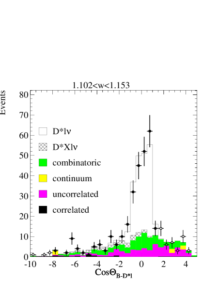
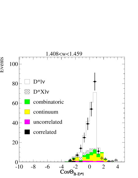
FIG. 2.: The event yields (circles) in the third and ninth $w$ bins with the results of the fit superimposed. The fit range is $-8\leq\mbox{$\cos\theta_{B-D^{*}\ell}$}<1.5$, and is indicated with the solid circles.

FIG. 3.: The $D^{*}\ell\nu$ and $\mbox{$D^{*+}$}X\ell\nu$ yields in each $w$ bin.

In order to test the quality of our fit and modeling of the signal and backgrounds, we plot a variety of distributions. Figure 4 shows the $D^{*}$ energy distribution and the lepton momentum spectrum. We find good agreement between the data and our expectations.

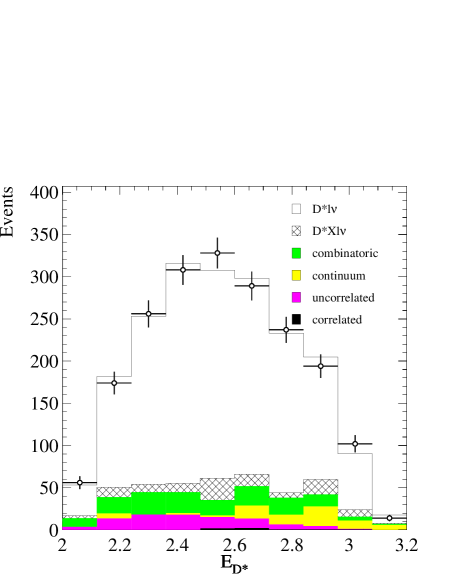
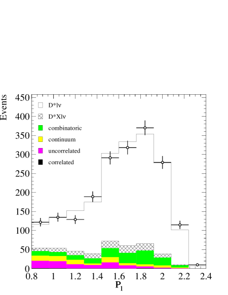
FIG. 4.: The energy distribution of $D^{*+}$ candidates (left) and the lepton momentum spectrum for $D^{*+}\ell\nu$ candidates (right) in the signal region for all $w$ bins combined.

V The $|V_{cb}|$ Fit

The partial width for $B\to\mbox{$D^{*}\ell\nu$}$ decays is given by [8]

$$\frac{d\Gamma}{dw}=\frac{G_{F}^{2}}{48\pi^{3}}(m_{B}-m_{D^{*}})^{2}m_{D^{*}}^{3}\sqrt{w^{2}-1}(w+1)^{2}\left(1+4\left(\frac{w}{w+1}\right)\left(\frac{1-2wr+r^{2}}{(1-r)^{2}}\right)\right)\left[\mbox{$|V_{cb}|$}F(w)\right]^{2}$$ (2)

where $m_{B}$ and $m_{D^{*}}$ are the $B$ and $D^{*}$ meson masses, $r=m_{D^{*}}/m_{B}$, and the form factor $F(w)$ is given by

$$F(w)=\sqrt{\frac{\tilde{H}^{2}_{0}+\tilde{H}^{2}_{+}+\tilde{H}^{2}_{-}}{1+4\left(\frac{w}{w+1}\right)\left(\frac{1-2wr+r^{2}}{(1-r)^{2}}\right)}}h_{A_{1}}(w).$$ (3)

The $\tilde{H}_{i}$ are the helicity form factors and are given by

$$\tilde{H}_{0}(w) = 1+\frac{w-1}{1-r}(1-R_{2}(w))$$ (4)

$$\tilde{H}_{+}(w) = \frac{\sqrt{1-2wr+r^{2}}}{1-r}\left(1-\sqrt{\frac{w-1}{w+1}}R_{1}(w)\right)$$ (5)

$$\tilde{H}_{-}(w) = \frac{\sqrt{1-2wr+r^{2}}}{1-r}\left(1+\sqrt{\frac{w-1}{w+1}}R_{1}(w)\right).$$ (6)

The form factor $h_{A_{1}}(w)$ and the form factor ratios $R_{1}(w)=h_{V}(w)/h_{A_{1}}(w)$ and $R_{2}(w)=(h_{A_{3}}(w)+rh_{A_{2}}(w))/h_{A_{1}}(w)$ have been studied both experimentally and theoretically. A CLEO analysis [3] measured these form factors under the assumptions that $h_{A_{1}}(w)$ is linear as a function of $w$ and that $R_{1}$ and $R_{2}$ are independent of $w$. CLEO found

$$R_{1} = 1.18\pm 0.30\pm 0.12,$$ (7)

$$R_{2} = 0.71\pm 0.22\pm 0.07{\rm\ and}$$ (8)

$$-\frac{dh_{A_{1}}}{dw}(w=1)\equiv\rho^{2} = 0.91\pm 0.15\pm 0.06$$ (9)

with the correlation coefficients $C(\rho^{2},R_{1})=0.60$, $C(\rho^{2},R_{2})=-0.80$ and $C(R_{1},R_{2})=-0.82$.

$R_{1}(1)$ and $R_{2}(1)$ have been computed using HQET and QCD sum rules with the results $R_{1}(1)=1.27$ and $R_{2}(1)=0.8$ and estimated errors of $0.1$ and $0.2$ respectively [11], in good agreement with the experimental results. $R_{1}(w)$ and $R_{2}(w)$ are expected to vary weakly with $w$. Most importantly for this analysis, $F(1)(=h_{A_{1}}(1))$ is relatively well-known, thereby allowing us to disentangle it from $|V_{cb}|$. We will use $F(1)=0.913\pm 0.042$ [12].

Recently, dispersion relations have been used to constrain the shapes of the form factors[13], [14]. Rather than expand the form factor in $w$, these analyses expand in the variable $z=(\sqrt{w+1}-\sqrt{2})/(\sqrt{w+1}+\sqrt{2})$. Ref. [13] obtains the results:

$$h_{A_{1}}(w) = 1-8\rho^{2}z+(53\rho^{2}-15)z^{2}-(231\rho^{2}-91)z^{3}$$ (10)

$$R_{1}(w) = R_{1}(1)-0.12(w-1)+0.05(w-1)^{2}$$ (11)

$$R_{2}(w) = R_{2}(1)+0.11(w-1)-0.06(w-1)^{2}.$$ (12)

In our analysis, we assume that the form factor has the functional form derived from dispersion relations given in Equations 10, 11 and 12. We fit our yields as a function of $w$ for $F(1)$$|V_{cb}|$ and $\rho^{2}$, keeping $R_{1}(1)$ and $R_{2}(1)$ fixed at their measured values. Our fit minimizes

$$\chi^{2}=\sum_{i=1}^{10}\frac{[N_{i}^{obs}-\sum_{j=1}^{10}\epsilon_{ij}N_{j}]^{2}}{\sigma_{N_{i}^{obs}}^{2}},$$ (13)

where $N_{i}^{obs}$ is the yield in the $i^{{\rm th}}$ $w$ bin, $N_{j}$ is the number of decays in the $j^{{\rm th}}$ $w$ bin, and the matrix $\epsilon_{ij}$ accounts for the reconstruction efficiency and the smearing in $w$. Explicitly,

$$N_{j}=4f_{00}N_{\Upsilon(4S)}{\cal B}(\mbox{$D^{*+}$}\to D^{0}\pi^{+}){\cal B}(D^{0}\to K^{-}\pi^{+})\tau_{B^{0}}\int_{w_{j}}dw\frac{d\Gamma}{dw}$$ (14)

where $\tau_{B^{0}}$ is the $B^{0}$ lifetime [15], ${\cal B}(\mbox{$D^{*+}$}\to D^{0}\pi^{+})$ is the $\mbox{$D^{*+}$}\to D^{0}\pi^{+}$ branching fraction [15], ${\cal B}(D\to K\pi)$ is the $D^{0}\to K^{-}\pi^{+}$ branching fraction [15], $N_{\Upsilon(4S)}$ is the number of $\Upsilon(4S)$ events in the sample, and $f_{00}$ represents the $\Upsilon(4S)\to B^{0}\bar{B}^{0}$ branching fraction [16]. We use the result of Ref. [16] for $f_{00}$ as a constraint in the fit.

The result of the fit is shown in Figure 5. We find

$$|V_{cb}|F(1) = 0.0424\pm 0.0018$$ (15)

$$\rho^{2} = 1.67\pm 0.11{\rm\ and}$$ (16)

$$\chi^{2} = 3.1/8{\rm\ dof.}$$ (17)

with a correlation coefficient between $\mbox{$|V_{cb}|$}F(1)$ and $\rho^{2}$ of 0.90. These parameters give $\Gamma=0.0366\pm 0.0018\mbox{\ ${\rm ps}^{-1}$}$. The quality of the fit is excellent. We note that the slope is higher than that found in the previous CLEO analysis [17] because of the curvature introduced into our form factor. If we use a linear form factor and the same subset of the data, we obtain results compatible with the earlier analysis.

FIG. 5.: The results of the fit to the $w$ distribution. The upper figure shows the yields (solid circles) with the results of the fit superimposed (histogram). The lower figure displays $\mbox{$|V_{cb}|$}F(w)$, where the data points (solid circles) are derived from the yields after correcting for efficiency, smearing, and all terms in the differential decay rate apart from $\mbox{$|V_{cb}|$}F(w)$. The curve shows the result of the fit.

VI Systematic Uncertainties

The systematic uncertainties are summarized in Table I. The dominant systematic uncertainties arise from our background estimations and from our knowledge of the slow pion reconstruction efficiency.

A Background uncertainties

We test our procedure for subtracting combinatoric background by applying it to Monte Carlo simulated events. We assign a systematic error based on the difference between the results obtained using the “true” background and those obtained using the same procedure that we apply to our data. We also include the statistical uncertainty of the study.

The main source of uncertainty from the uncorrelated background is the normalization of the various contributions. Of these, the most important is the branching fraction of the $B\to D^{(*)}D^{*}K^{(*)}$ decays, which we vary by 50%. Smaller effects arise from the primary and secondary lepton rates and from the uncertainty in $B^{0}-\bar{B}^{0}$ mixing.

We assess the uncertainty arising from the correlated background by varying the branching fractions of the contributing modes.

B Slow $\pi$ reconstruction uncertainty

A major source of uncertainty for the analysis is the efficiency for reconstructing the slow pion from the $D^{*}$ decay. This efficiency is low near $w=1$ and increases rapidly over the next few $w$ bins. We have explored the efficiency as a function of the event environment and as a function of hit resolution, hit efficiency, material, and the charge division resolution in one of the inner drift chambers. The last of these is important because very soft tracks often make use of the charge division information for reconstruction of the $z$ component (beam direction) of their trajectory. The uncertainty in $|V_{cb}|$$F(1)$ and the decay width are dominated by uncertainties in the amount of material in the inner detector (2.3%) and the drift chamber hit efficiency (0.8%).

C Other uncertainties

The efficiency for identifying electrons has been evaluated using radiative bhabha events embedded in hadronic events, and has an uncertainty of 2.4%. Similarly, the muon identification efficiency has been evaluated using radiative mu-pair events, and has an uncertainty of 1.4%. The total uncertainty in lepton identification, weighted by the electron and muon populations, is 2.1%. Separate electron and muon analyses of our data give consistent results.

The $B^{0}$ momentum is measured directly in the data using fully reconstructed hadronic decays, and is known on average with a precision of 0.0016  MeV. Variation of the momentum in our reconstruction slightly alters the $\cos\theta_{B-D^{*}\ell}$ distribution that we expect for our signal, and it therefore changes the yields obtained from the $\cos\theta_{B-D^{*}\ell}$ fits. Likewise, CLEO has measured the $B^{0}$ meson mass [18] and when we vary the mass within its measurement error, we find a small effect on the yields.

We determine the tracking efficiency uncertainties for the lepton and the $K$ and $\pi$ forming the $D^{0}$ in the same study used for the slow pion from the $D^{*+}$ decay. These uncertainties are confirmed in a study of 1-prong versus 3-prong $\tau$ decays.

Finally, our analysis requires that we know the $\cos\theta_{B-D^{*}\ell}$ distribution of the $D^{*}X\ell\nu$ contribution. This distribution in turn depends on both the branching fractions of contributing modes and on their form factors. Variation of all of these branching fractions and form factors is not only cumbersome, but out of reach given the poor current knowledge of these modes. Instead, we note that the $B\to D^{*}\pi\ell\nu$ and $B\to D_{1}\ell\nu$ modes are the ones with the most extreme $\cos\theta_{B-D^{*}\ell}$ distributions (the largest mean and the smallest). These distributions are shown in Figure 6. We therefore repeat the analysis, first using pure $B\to D^{*}\pi\ell\nu$ to describe our $D^{*}X\ell\nu$ decays and then using pure $B\to D_{1}\ell\nu$ to describe these decays, and we take the larger of the two excursions as our systematic error.

FIG. 6.: The $\cos\theta_{B-D^{*}\ell}$ distribution of the $B\to D^{*+}\pi\ell\nu$ (left) and $B\to D_{1}\ell\nu$ (right) events contributing to the $D^{*+}\ell\nu$ sample.

D Sensitivity to $R_{1}(1)$ and $R_{2}(1)$

The form factor ratios $R_{1}(1)$ and $R_{2}(1)$ affect the lepton spectrum and therefore the fraction of events satisfying our 0.8 GeV electron and 1.4 GeV muon momentum requirements. To assess this effect, we vary $R(1)$ and $R(2)$ within their measurement errors, taking into account the correlation between them.

TABLE I.: The fractional systematic uncertainties.

Source	$|V_{cb}|F(1)$(%)	$\rho^{2}$(%)	$\Gamma(B\to\mbox{$D^{*+}\ell\nu$})$(%)
Combinatoric Background	1.4	1.8	1.2
Uncorrelated Background	0.7	0.9	0.7
Correlated Background	0.4	0.3	0.5
Slow $\pi$ finding	3.1	3.7	2.9
$K$, $\pi$ & $\ell$ finding	1.0	0.0	1.9
Lepton ID	1.1	0.0	2.1
$B$ momentum & mass	0.3	0.5	0.4
$D^{*}X\ell\nu$ model	0.2	1.9	1.9
Number of $B\bar{B}$ events	0.9	0.0	1.8
Subtotal	3.8	4.7	5.0
${\cal B}(D^{*}\to D\pi)$	0.4	0.0	0.7
${\cal B}(D\to K\pi)$	1.2	0.0	2.3
$\tau_{B}$	1.0	0.0	2.1
$R_{1}(1)$ and $R_{2}(1)$	1.4	12.0	1.8
Subtotal	2.1	12.0	3.7
Total	4.4	13	6.2

VII Conclusions

We have fit the $w$ distribution of $B\to\mbox{$D^{*}\ell\nu$}$ decays for the slope of the form factor and $|V_{cb}|F(1)$. We find

$$|V_{cb}|F(1) = 0.0424\pm 0.0018\pm 0.0019$$ (18)

$$\rho^{2} = 1.67\pm 0.11\pm 0.22$$ (19)

with a correlation coefficient between $\mbox{$|V_{cb}|$}F(1)$ and $\rho^{2}$ of 0.90. These parameters imply the decay rate

$$\Gamma=0.0366\pm 0.0018\pm 0.0023\mbox{\ ${\rm ps}^{-1}$}.$$ (21)

and the branching fraction

$${\cal B}(B\to\mbox{$D^{*+}\ell\nu$})=(5.66\pm 0.29\pm 0.33)\%.$$ (22)

Our result implies

$$\mbox{$|V_{cb}|$}=0.0464\pm 0.0020(stat.)\pm 0.0021(syst.)\pm 0.0021(theor.),$$ (23)

where we have used $F(1)=0.913\pm 0.042$ [12]. This is consistent with previous measurements of $|V_{cb}|$, but is somewhat higher. The analysis benefits from small backgrounds and good resolution in $w$. These results are preliminary.

VIII Acknowledgements

We are indebted to the CESR staff for the superb performance of the accelerator. I.P.J. Shipsey thanks the NYI program of the NSF, M. Selen thanks the PFF program of the NSF, A.H. Mahmood thanks the Texas Advanced Research Program, M. Selen and H. Yamamoto thank the OJI program of DOE, M. Selen and V. Sharma thank the A.P. Sloan Foundation, M. Selen and V. Sharma thank the Research Corporation, F. Blanc thanks the Swiss National Science Foundation, and H. Schwarthoff and E. von Toerne thank the Alexander von Humboldt Stiftung for support. This work was supported by the National Science Foundation, the U.S. Department of Energy, and the Natural Sciences and Engineering Research Council of Canada.

REFERENCES

- [1] Y. Kubota et al. (CLEO Collaboration), Nucl. Instrum. Methods Phys. Res., Sect. A 320, 66 (1992).
- [2] R. Brun et al., GEANT 3.15, CERN DD/EE/84-1.
- [3] J Duboscq et al.(CLEO Collaboration) PRL 76, 3898 (1996).
- [4] E Barberio and Z Was, Comput. Phys. Commun. 79, 291 (1994).
- [5] JL Goity and W Roberts, Phys. Rev. D 51, 3459 (1995).
- [6] D Scora and N Isgur, Phys. Rev. D 52, 2783 (1995); N Isgur et al., Phys. Rev. D 39, 799 (1989).
- [7] Routine HMCLNL, described in the HBOOK manual(CERN); Roger Barlow and Christine Beeston, Comp. Phys. Comm. 77, 219 (1993).
- [8] JD Richman and PR Burchat, Rev. Mod. Phys., 67, 893 (1995).
- [9] B Barish et al.(CLEO Collaboration), Phys. Rev. Lett. 76, 1570 (1996).
- [10] BH Behrens et al.(CLEO Collaboration), CLNS 00/1668.
- [11] M. Neubert, Physics Reports, 245, 259 (1994).
- [12] BaBar Physics Book, PF Harrison and HR Quinn, editors, SLAC-R-504 (1998).
- [13] I Caprini,L Lellouch and M Neubert, Nucl. Phys. B 530, 153 (1998) (hep-ph/9712417).
- [14] CG Boyd, B Grinstein, RF Lebed, Phys. Rev. D 56, 6895 (1997) (hep-ph/9705252).
- [15] We use DE Groom et al., Eur. Phys. Jrnl, C15, 1 (2000).
- [16] JP Alexander et al.(CLEO Collaboration), CLNS 00/1670 (2000).
- [17] B Barish et al.(CLEO Collaboration), Phys. Rev. D 51, 1014 (1995).
- [18] SE Csorna et al.(CLEO Collaboration), Phys. Rev. D 61, 111101 (2000)(hep-ex/0001013).