Setting Confidence Belts

Abstract

We propose using a Bayes procedure with uniform improper prior to determine credible belts for the mean of a Poisson distribution in the presence of background and for the continuous problem of measuring a non-negative quantity $\theta$ with a normally distributed measurement error. Within the Bayesian framework, these belts are optimal. The credible limits are then examined from a frequentist point of view and found to have good frequentist and conditional frequentist properties.

I Introduction

We consider two simple problems for setting confidence belts. The first problem is that of the Poisson distribution in the presence of background. The second problem is the measurement of a non-negative parameter $\theta$, with a normally distributed error. Although simple problems, there has been considerable work and discussion on them in the last few years. Most of the discussion has centered on the Poisson case, when the number of observed events is small. This is an important current topic because there are many search experiments involving small numbers of events. These include Higgs particle searches, supersymmetry searches, and neutrino oscillation searches such as LSND and KARMEN.

We will briefly describe some recent attempts to address these problems.

II The Feldman-Cousins Unified Approach

The standard method for setting 90% CL bounds has been to select a region with a 5% probability above and a 5% probability below the bounds. About two years ago, Gary Feldman and Bob Cousins[1] suggested a method, new to physics analyses, called the unified procedure. For the Poisson case, for each possible value of the parameter $\theta$, they looked at the ratio of the probability of getting the observed number of events $n$ for that $\theta$ compared to the maximum probability for all physically allowed $\theta$’s, and picked $n$’s with the highest ratio to build a 90% confidence region. This solved two problems with the old procedure. It automatically transitioned from an upper limit to a confidence belt and it always produced confidence sets in the physical region.

The unified procedure works well for many problems and is a significant improvement over the symmetric tails procedure. However it has a serious problem if few or no events are observed. If 0 events are seen, there are 0 signal and 0 background events. That there are 0 background events is interesting, but irrelevant to the question of whether signal events are seen. A 90% C.L. limit on $\theta$ should come from $p_{\theta}(0)\leq 10$%, which sets a limit at $\theta=2.3$. (Throughout this article probabilities for a fixed parameter $\lambda$ are denoted by a subscript $p_{\lambda}$. Probability densities and probability masses are denoted with lower case letters and distribution functions by upper case letters.) Such a case did occur in the Summer of 1998 from initial KARMEN results [2]. They had 0 events with a background of 2.88, and using the unified method obtained an upper limit of $\theta=1.08$. It is desirable to have a method set a confidence limit near 2.3, independent of background, for a 90% C.L., when no events are seen.

III The Roe-Woodroofe Procedure

We [3] presented a variant of the Feldman-Cousins unified procedure which corrected this problem and introduced the concept of conditional coverage. For any observation we know that the background is less or equal to the observed number of events, $n_{observed}$. We suggested the use of a sample space not of all experimental outcomes, but of outcomes with background $\leq n_{observed}$. Thus, if $n_{observed}=4$, we considered only measurements in which there are $\leq 4$ background events, even for 20 events observed in the sample space. This probability was used both to set the ratio used in the unified method and to calculate the coverage probability. This method had the advantage of giving an upper limit of about 2.42 for 0 observed events independently of the background mean $b$. See Figure 1.

Robert Cousins [4] found that this procedure had a problem with its lower limit when applied to a continuous observable. Suppose one measures a parameter $\theta\geq 0$ with a measurement error $\Delta,\ x=\theta+\Delta$, where $\Delta$ is normal (0,1). The R-W procedure eliminated $\theta=0$ for all $x>0$. However, if $\theta=0$, the probability of measuring $x>1.39$ is 10%. See Figure 2. It appeared that the R-W upper limit and the F-C lower limit were needed.

Since the conditional coverage concept is, as yet, unfamiliar, it is desirable that a method should have reasonable conventional coverage as well as conditional coverage.

IV Bayesian Credible Intervals

In this section, we derive Baysian credible intervals when the expected signal is given a uniform prior distribution. These intervals have several desirable properties. Like the unified intervals, Bayesian intervals lie in the physical region and automatically change from confidence bounds to two-sided intervals. They avoid the known pitfalls mentioned above, the problems with low counts in unified method and the large lower boundary of the conditional confidence intervals in the continuous case. Finally, and importantly, the Bayesian intervals are optimal on their own terms. The intervals derived minimize length among all credible intervals. The price paid for these desirable properties is dependence on the prior and metric. We address the first of these concerns by showing that the frequentist coverage probability of the Bayesian intervals is quite close to the Bayesian posterior credible level. That is, while the two probabilities are conceptually quite different, they are close numerically. In addition, we show that the Bayesian credible intervals have exact conditional (frequentist) coverage probability, except for discreteness in the Poisson case. With regard to the metric, it is primarily the optimality of our procedures that depends on the metric. See Section 7.

We will illustrate with two examples, a Poisson case in which the mean is composed of an unknown signal mean $\theta\geq 0$ and a known background mean $b$ and the measurement $x$ of a parameter $\theta\geq 0$, with a measurement error $\Delta$ which is normal (0,1). We use a uniform (improper) prior of 1 for $0\leq\theta<\infty$ in both problems.

A The Continuous Example

This is a simple problem in which the statistical issues are clear and which approximates the Poisson problem for large $b+\theta$. We measure $x=\theta+\Delta$, where $\theta\geq 0$, and the density function for $x$ is

$$f(x|\theta)\equiv\phi(x-\theta)={1\over\sqrt{2\pi}}e^{-{1\over 2}(x-\theta)^{2}}.$$ (1)

For the uniform prior probability $pr(\theta)=1$, the marginal density of $x$ becomes

$$f(x)=\int_{0}^{\infty}\phi(x-\theta)pr(\theta)d\theta=\Phi(x),$$

where

$$\Phi(x)\equiv\int_{-\infty}^{x}\phi(y)dy,$$

the standard normal distribution function. We now use Bayes theorem $f(x|\theta)\times pr(\theta)=f(\theta|x)\times f(x)$. The conditional density of $\theta$ given $x$ is

$$f(\theta|x)={\phi(x-\theta)\over\Phi(x)}.$$ (2)

$f(\theta|x)$ is proper; the improper (infinite) prior has cancelled out. We wish to find an upper limit $u$ and a lower limit $\ell$, dependent on $x$, for which

$$Prob\{\ell\leq\theta\leq u|x\}=1-\epsilon.$$ (3)

In Bayes theory, such intervals are called credible intervals. It is desirable to minimize the interval $[\ell,u]$, subject to (3). We do that by picking $\theta$’s with the largest probability density to be within the interval,

$$[\ell,u]=\{\theta:f(\theta|x)\geq c\},$$

where $0\leq c\leq 1/\sqrt{2\pi}$ is chosen to satisfy Equation (3). Now, $f(\theta|x)\geq c$ if and only if $|\theta-x|\leq d$, where

$$d=\sqrt{-2\ln c-\ln(2\pi)-2\ln[\Phi(x)]}.$$

There are two cases to be considered. If $d\leq x$, then the condition (3) becomes

$$1-\epsilon=\int_{x-d}^{x+d}f(\theta|x)d\theta=\int_{-d}^{d}{\phi(\omega)\over\Phi(x)}d\omega={2\Phi(d)-1\over\Phi(x)};$$

$$d=\Phi^{-1}[{1\over 2}+{1\over 2}(1-\epsilon)\Phi(x)],$$ (4)

where $\Phi^{-1}$ denotes the inverse function to $\Phi$. If $x<d$, (3) becomes

$$\epsilon=\int_{x+d}^{\infty}f(\theta|x)d\theta=\int_{d}^{\infty}{\phi(\omega)\over\Phi(x)}d\omega={1-\Phi(d)\over\Phi(x)};$$

$$d=\Phi^{-1}[1-\epsilon\Phi(x)].$$ (5)

If $x_{0}$ is the point where these two curves meet, then,

$$x_{0}=\Phi^{-1}\left({1\over 1+\epsilon}\right).$$ (6)

Hence, the desired credible interval is $[\ell,u]=[\max(x-d,0),x+d],$ where $d=\Phi^{-1}[1-\epsilon\Phi(x)]$, if $-\infty<x\leq x_{0}$, and $d=\Phi^{-1}[{{1\over 2}}+{{1\over 2}}(1-\epsilon)\Phi(x)]$ if $x_{0}<x<\infty$.

B Poisson Example

The probability mass function and distribution function for the Poisson distribution with mean $\lambda$ are:

$$p_{\lambda}(n)={e^{-\lambda}\lambda^{n}\over n!}.$$ (7)

and $P_{\lambda}(n)=p_{\lambda}(0)+\cdots+p_{\lambda}(n)$. For our present problem $\lambda=\theta+b$, where $b\geq 0$ is the fixed (known) “background” mean. If we let $\theta$ have a prior uniform distribution $pr(\theta)=1$ for $\theta\geq 0$, we then have

$$p(n)=\int_{0}^{\infty}{1\over n!}(\theta+b)^{n}e^{-(\theta+b)}pr(\theta)d\theta$$

$$=\int_{b}^{\infty}{1\over n!}\omega^{n}e^{-\omega}d\omega=P_{b}(n)$$ (8)

as derived in our previous paper[3]. The derivation proceeded by expanding $(\theta+b)^{n}$ and noting that $\int_{0}^{\infty}\theta^{k}e^{-\theta}d\theta=k!$. We again use Bayes’ Theorem $p_{\theta+b}(n)\times pr(\theta)=p_{b}(n,\theta)=p_{b}(\theta|n)\times p(n)$. Then, recalling that $pr(\theta)=1$ for $\theta\geq 0$ and $p(n)=P_{b}(n)$, we have

$$p_{b}(\theta|n)={p_{\theta+b}(n)\over P_{b}(n)}.$$ (9)

To set upper and lower confidence bounds for $\theta$, we need to solve the equation

$$1-\epsilon=\int_{\ell}^{u}p_{b}(\theta|n)d\theta={P_{b+\ell_{n}}(n)-P_{b+u_{n}}(n)\over P_{b}(n)}$$ (10)

for $\ell$ and $u$. A 90% C.L. corresponds to setting $\epsilon=0.1$. The second equality here is obtained by writing $\int_{\ell}^{u}=\int_{\ell}^{\infty}-\int_{u}^{\infty}$ and using the reasoning described after Equation (8). To get the shortest interval $u-\ell$ we need to include values of $\theta$ with highest density, i.e.,

$$[\ell,u]=[\theta:p_{b}(\theta|n)\geq c]$$ (11)

for some $c$. The conditions (10) and (11) may be solved numerically by an iterative procedure. This procedure is described in Section 6 in a more general context.

V Frequentist Properties

The Bayesian credible intervals just derived have exact posterior coverage probability $1-\epsilon$, by construction. In this section, we show that they also have high frequentist coverage probability.

A The Continuous Example

In the continuous example, $x=\theta+\Delta,\theta\geq 0$, and $\Delta\sim{\rm normal}(0,1)$. Fix a $\theta$ and find the points at this fixed $\theta$ where $x$ meets the upper and lower Bayesian limits. Let $x_{\ell}(\theta)$ be that $x$ which meets the upper limit, $\theta=u(x_{\ell})=x_{\ell}+d(x_{\ell})$ and $x_{u}(\theta)$ be that $x$ which meets the lower limit, $\theta=\ell(x_{u})=x_{u}-min[d(x_{u}),x_{u}]$. Then $[\ell(x),u(x)]$ covers $\theta$ iff $x_{\ell}\leq x\leq x_{u}$, and the conventional unconditional coverage is $\Phi(x_{u}-\theta)-\Phi(x_{\ell}-\theta)$. This is not exactly $1-\epsilon$. A lower limit on the coverage is shown in the Appendix to be

$$\Phi(x_{u}-\theta)-\Phi(x_{\ell}-\theta)\geq{1-\epsilon\over 1+\epsilon},$$ (12)

but this is a very conservative limit. For $\epsilon=0.1$, this lower limit is 0.8182, while a numerical calculation finds a minimum coverage of about 0.86.

The conventional coverage probability can be improved for a very small increase in limits. We will consider a conservative ad-hoc modification of the upper limit on $\theta$ using the one-sided limit for a higher confidence level, $\epsilon^{\prime}=\epsilon/2$. Let

$$u^{\prime}(x)=\max\left[u(x),x+\Phi^{-1}\left(1-{1\over 2}\epsilon\right)\right].$$

Let $x^{\prime}_{\ell}$ be the $x$ corresponding to $u^{\prime}(x)=\theta$. The formula for the conventional coverage is $\Phi(x_{u}-\theta)-\Phi(x^{\prime}_{\ell}-\theta)$, as above. The undercoverage, derived in the Appendix, is very small for this conservative modification. For a 90% C.L., the conventional coverage is at least .900 everywhere to three significant figures. Figure 3 shows a plot of the coverage bands, plotted as $\theta-x$ vs $x$. The confidence bands are shown in Figure 4 and compared with the old R-W upper bound and the Feldman-Cousins unified procedure lower bound. The conventional frequentist coverage for the Bayesian model and for this conservative modification are shown in Figure 5.

The Bayesian credible intervals also have an exact conditional frequentist property, in terms of the error $\Delta=x-\theta$. Note that if $x$ is observed, then, necessarily, $\Delta\leq x$, since $\theta\geq 0$. $\Phi(x)$ is just the probability that $\Delta\leq x$. Let $a(x)=min[d(x),x]$. Then the interval $[\ell(x),u(x)]$ covers $\theta$ iff $\ell(x)\leq\theta\leq u(x)$ or, equivalently, $-d(x)\leq\Delta\leq a(x)$. In the Appendix, it is shown that if $x^{\prime}=\theta+\Delta^{\prime}$ is an independent copy of $x$, then

$$Prob_{\theta}[-d(x)\leq\Delta^{\prime}\leq a(x)|\Delta^{\prime}\leq x]=1-\epsilon$$

and $[\ell(x),u(x)]$ is the shortest interval with these properties.

B The Poisson Example

As in the continuous case, the conventional coverage is not exact in the Poisson case. For $b=3$ and $1-\epsilon=0.9$, for example, the conventional coverage varies from about 86% to 96.6%. Figure 6 shows the resulting confidence belt for $b=3,\ \epsilon=0.1$.

The conditional coverage is shown in the Appendix to be $\approx 1-\epsilon$, except for discreteness.

The conventional coverage can be improved by a small ad hoc modification similar to that used for the continuous case. Consider an alternate Bayesian upper limit $u^{\prime}$ for $\theta$ defined as the one-sided limit for a credible level $=1-\epsilon^{\prime}$. Take the modified upper limit as the maximum of $u$ and $u^{\prime}$. In the continuous example we chose $\epsilon^{\prime}=\epsilon/2$. Here, we make a different ad hoc choice. The effect of the modification for $b=3,\ \epsilon=0.1$ and $\epsilon^{\prime}=0.08$ is shown in Figure 7. The value of the limit for $n=0$ then increases from 2.3 to 2.53. See Figure 8. For a fixed $\epsilon^{\prime}$ the limit at $n=0$ is independent of $b$, but the appropriate choice of $\epsilon^{\prime}$ will depend weakly on $b$.

VI Partial Background-Signal Separation

In this section, we extend the method to processes in which we have some information concerning whether a given event is a signal or a background event. Suppose on each event one measures a statistic $x$ (or a vector of statistics) for which the density function is $g(x)$ for signal events and $h(x)$ for background events. Suppose, further, that the number of observed events $n$ has a Poisson distribution with mean $b+\theta$, where $\theta$ is the expected number of signal events. We assume that $b$, the expected number of background events, is known. Then the joint probability mass function/density for observing $n$ events and parameters $x_{1},\cdots,x_{n}$ is

$$f_{\theta}(n,x)={(b+\theta)^{n}\over n!}e^{-(b+\theta)}\prod_{k=1}^{n}\left[{\theta g(x_{k})+bh(x_{k})\over b+\theta}\right]$$

$$={1\over n!}e^{-(b+\theta)}\prod_{k=1}^{n}[b+\theta r(x_{k})]\times\prod_{k=1}^{n}h(x_{k}),$$ (13)

where $r(x_{k})=g(x_{k})/h(x_{k})$. For a uniform prior, $pr(\theta)=1$ for $0\leq\theta<\infty$, the marginal and posterior probability mass function/densities of $n$ and $x_{1},\cdots,x_{n}$, and of $\theta$ are then

$$f(n,x) = \int_{0}^{\infty}f_{\theta}(n,x)d\theta$$

$$= {1\over n!}\prod_{k=1}^{n}h(x_{k})\times\int_{0}^{\infty}e^{-(b+\theta)}\prod_{k=1}^{n}[b+\theta r(x_{k})]e^{-(b+\theta)}d\theta$$

$$q(\theta|n,x)={f_{\theta}(n,x)\over f(n,x)}.$$ (14)

Observe that

$$\int_{0}^{\infty}e^{-(b+\theta)}\prod_{k=1}^{n}[b+\theta r(x_{k})]d\theta=n!\sum_{m=0}^{n}C_{n,m}{b^{n-m}\over(n-m)!}e^{-b},$$

where

$$C_{n,m}=\left[1/\left({n\atop m}\right)\right]\sum_{j_{1}+\cdots+j_{n}=m}\prod_{k=1}^{n}r(x_{k})^{j_{k}},$$ (15)

and where $j_{1}\cdots j_{n}$ are restricted to the values 0 or 1. Cancelling common factors,

$$q(\theta|n,x)={e^{-\theta}\prod_{k=1}^{n}[b+\theta r(x_{k})]\over n!\sum_{m=0}^{n}C_{n,m}{b^{n-m}\over(n-m)!}}.$$ (16)

Observe also that if $g=h$, then $C_{n,m}=1$ and $q(\theta|n,x)$ is the same as the posterior density of $\theta$ given $n$ in the Poisson case without the extra variables $x$.

We want to find upper and lower limits $u,\ell$ for $\theta$ such that $Prob\{\ell\leq\theta\leq u|n,x\}=1-\epsilon$ and to minimize that interval. This means we want $[\ell,u]=\{\theta:q(\theta|n,x)\geq c\}$. We first find the value $\theta_{max}$ at which $q(\theta|n,x)$ is maximum, or, equivalently, $\ln[q(\theta|n,x)]$ is maximum. Since the denominator in Equation (16)

$$D=n!\sum_{m=0}^{n}{b^{n-m}\over(n-m)!}C_{n,m}$$ (17)

does not depend on $\theta$,

$${d\over d\theta}\ln[q(\theta|n,x)]=\sum_{k=1}^{n}{r(x_{k})\over b+\theta r(x_{k})}-1.$$

If $r(x_{1})\cdots r(x_{n})<b$, then $\theta_{max}=0$. Otherwise, setting the derivative equal to 0 then leads to the equation

$$\theta_{max}=\sum_{k=1}^{n}{\theta_{max}r(x_{k})\over b+\theta_{max}r(x_{k})}.$$ (18)

If $g=h$, then it is easy to see that $\theta_{max}=\max[0,n-b]$. It is clear from (18) that $\theta_{max}\leq n$, and it can be shown that the obvious iteration starting at $\theta=n$ converges to $\theta_{max}$. This iteration is a special case of the EM algorithm [5].

Next integrate $q(\theta|n,x)$. Let

$$Q(a|n,x)\equiv\int_{0}^{a}q(\theta|n,x)d\theta.$$

Then

$$1-Q(a|n,x)={1\over D}\int_{a}^{\infty}e^{-\theta}\prod_{i=1}^{n}[b+\theta r(x_{i})]d\theta$$

$$={1\over D}\sum_{m=0}^{n}b^{n-m}C_{n,m}\left({n\atop m}\right)\int_{a}^{\infty}\theta^{m}e^{-\theta}d\theta.$$ (19)

We use the reasoning described after Equation(8) to evaluate this integral.

$$1-Q(a|n,x)={1\over D}\sum_{m=0}^{n}b^{n-m}C_{n,m}{n!\over m!(n-m)!}m!e^{-a}\sum_{l=0}^{m}{a^{l}\over l!}$$

$$={e^{-a}\sum_{i=0}^{n}{b^{n-i}C_{n,i}\over(n-i)!}\sum_{l=0}^{i}{a^{l}\over l!}\over\sum_{m=0}^{n}{b^{n-m}\over(n-m)!}C_{n,m}}.$$ (20)

We can use either Equation (19), recognizing that the integral is an incomplete gamma function, or use Equation (20) to find $Q(a|n,x)$. The limits can then be found by iterations as follows.

1. First solve the equation $Q(z|n,x)=1-\epsilon$ for $z$. This is straightforward, since $Q(z|n,x)$ is increasing in $z$.

2. If $q(z|n,x)\leq q(0|n,x)$, then $\ell=0$ and $u=z$.

3. If $q(0|n,x)<q(z|n,x)$, solve the equations

$$q(y|n,x)=c,$$

$$q(z|n,x)=c,$$

$$Q(z|n,x)-Q(y|n,x)=1-\epsilon$$

for $c,y,z$ by a double iteration. In solving these equations, start with $c=(c_{min}+c_{max})/2$, where $c_{min}=q(0|n,x)$ and $c_{max}$ is the maximum value of $q(\theta|n,x)$, corresponding to $\theta=\theta_{max}$. Solve the first two equations for $y<\theta_{max}<z$. This is straightforward, since $q(\theta|n,x)$ is increasing for $\theta\leq\theta_{max}$ and decreasing for $\theta>\theta_{max}$. Then replace $c_{max}$ (respectively, $c_{min}$) by $c$, accordingly as $Q(z|n,x)-Q(y|n,x)<1-\epsilon$ (respectively, $>1-\epsilon$).

Note that the iteration procedure for the Poisson example without additional parameters measured is just a special case of this iteration procedure.

VII Concluding Remarks

We have proposed methods for setting credible/confidence intervals for the means $\theta$ of a Poisson variable, observed in the presence of background, and of a normal distribution, when $\theta$ is known to be non-negative. In the process, we have made specific choices for the prior distributions and loss structure. The (uniform) prior distributions were chosen for mathematical tractability and agreement between the Bayesian credible level and conventional confidence level; and one of the main findings is that such agreement is possible. The intervals have an optimality property: they minimize the length of credible intervals in the $\theta$ scale for the uniform prior. For both problems, the mean provides a physically meaningful and mathematically tractable metric. Our procedures depend on the choice of metric, prior, and loss structure as follows: if the interval for $\theta$ is $\ell\leq\theta\leq u$ and the metric were changed, to $\tau=1/\theta$ say, then a valid interval for $\tau$ is $1/u\leq\tau\leq 1/\ell$. This has the same frequentist coverage as the original interval and is an exact credible interval for the induced prior, $d\tau/\tau^{2}$. The optimality is lost, however. The transformed interval does not minimize length in the $\tau$-scale. The situation for our method is similar to that in the Cramer-Rao limit, Equation 13.10 of Roe [6]. This very useful bound also depends on the metric.

The derivations of the ad hoc modifications in Section 5 mix Bayesian and frequentist reasoning, and this may seem inelegant. We believe that any inelegance is mitigated by the minor nature of the changes and the resulting good properties of the procedure from both the Bayesian and frequentist viewpoints.

In the case of a Poisson distribution without auxiliary variables, there is a close connection between our method and $CL_{s}$: the $CL_{s}$ procedure is mathematically equivalent to an upper credible bound with a uniform prior distribution. Read [7] calls this a coincidence. We think that there is a deeper connection [8]. The optimality claimed for $CL_{b+s}$ in Read’s work is optimality for testing background only versus background plus a specified signal. Our procedures are designed to produce intervals of shortest length, not most powerful tests. That these two criteria can lead to different procedures was noted in the statistical literature by Pratt [9].

This research is supported by the National Security Agency under MDA904-99-1-004 and the National Science Foundation under PHY-9725921.

Proofs of Coverage and Optimality Theorems

1 Continuous Example

Recall that if $x=\theta+\Delta$ is observed, then necessarily $\Delta\leq x$ and that $\theta\in[\ell(x),u(x)]$ iff $-d(x)\leq\Delta\leq a(x)$, where $d(x)=u(x)-x$ and $a(x)=x-\ell(x)=min[d(x),x]$. Let $x^{\prime}=\theta+\Delta^{\prime}$ be an independent copy of $x$.

Theorem: For every $x,\ Prob_{\theta}[-d(x)\leq\Delta^{\prime}\leq a(x)|\Delta^{\prime}\leq x]=1-\epsilon$, and $[\ell(x),u(x)]$ is the shortest interval with this property. The first statement says that the conditional coverage of $x-\theta$ is exact.

Proof: The result follows from

$$Prob_{\theta}[\Delta^{\prime}\leq z|\Delta^{\prime}\leq x]={\Phi[min(x,z)]\over\Phi(x)}=Prob[x-\theta\leq z|x].$$ (21)

In words, the conditional frequentist distribution of $x^{\prime}-\theta$ is the same as the posterior distribution of $x-\theta$. It follows that

$$Prob_{\theta}[-d(x)\leq\Delta^{\prime}\leq a(x)|\Delta^{\prime}\leq x] = Prob[x-u(x)\leq x-\theta\leq min(x,d(x))|x]$$

$$= Prob[\ell(x)\leq\theta\leq u(x)|x]=1-\epsilon,$$

where the last equality follows from the definitions of $\ell(x)$ and $u(x)$. Next, if $[L(x),U(x)]$ is any interval for which $Prob_{\theta}[-D(x)\leq\Delta^{\prime}\leq A(x)|\Delta^{\prime}\leq x]=1-\epsilon$, where $D(x)=U(x)-x$ and $A(x)=x-L(x)$, then

$$Prob[L(x)\leq\theta\leq U(x)|x]=Prob[-D(x)\leq x-\theta\leq A(x)|x]=1-\epsilon$$

and, therefore, $U(x)-L(x)\geq u(x)-\ell(x)$, since the Bayesian limits were chosen to minimize the length of the interval.

$\diamondsuit$

To put this in more conventional terms, let the interval $C(x,x^{\prime})=[x^{\prime}-a(x),x^{\prime}+d(x)]$. Then

$$Prob_{\theta}[C(x,x^{\prime})\ni\theta|\Delta^{\prime}\leq x]=1-\epsilon,$$ (22)

where $x^{\prime}$ is the random variable.

Theorem: A lower limit for the conventional coverage is $(1-\epsilon)/(1+\epsilon)$.

Proof: Recall that $x_{\ell}$ and $x_{u}$ were the values of $x$ for a given $\theta$ meeting the upper and lower Bayesian limits, so $\theta=u(x_{\ell})=x_{\ell}+d(x_{\ell})$ and $\theta=\ell(x_{u})=x_{u}-min[d(x_{u}),x_{u}]$. The unconditional frequentist coverage probability is

$$Prob_{\theta}[\ell(x)\leq\theta\leq u(x)]=Prob_{\theta}[x_{\ell}\leq x\leq x_{u}]=\Phi(x_{u}-\theta)-\Phi(x_{\ell}-\theta).$$

Recall the definition of $x_{0}$ and observe that $x_{u}\geq x_{0}$ for all $\theta>0$, since $\theta=\ell(x_{u})$ and $\ell(x)=0$ for $x\leq x_{0}$. First suppose that $x_{\ell}\leq x_{0}$. Then $\Phi(x_{\ell})\leq\Phi(x_{0})\leq\Phi(x_{u})$ and $\Phi(x_{0})=1/(1+\epsilon)$ by (6). Also, by (4) and (5), $\Phi(x_{\ell}-\theta)=\Phi[-d(x_{\ell})]=1-\Phi[d(x_{\ell})]=\epsilon\Phi(x_{\ell}),\ \Phi(x_{u}-\theta)=\Phi[d(x_{u})]={1\over 2}+{1\over 2}(1-\epsilon)\Phi(x_{u}),$ and

$$`\Phi(x_{u}-\theta)-\Phi(x_{\ell}-\theta) = {1\over 2}+{1\over 2}(1-\epsilon)\Phi(x_{u})-\epsilon\Phi(x_{\ell})$$

$$\geq {1\over 2}+{1\over 2}{1-\epsilon\over 1+\epsilon}-{\epsilon\over 1+\epsilon}$$

$$\geq {1-\epsilon\over 1+\epsilon}.$$

Next suppose $x_{\ell}>x_{0}$. Then $\Phi(x_{u})\geq\Phi(x_{\ell})\geq\Phi(x_{0})$, $\Phi(x_{\ell}-\theta)=\Phi[-d(x_{\ell})]=1-\left[{1\over 2}+{1\over 2}\left(1-\epsilon\right)\Phi(x_{\ell})\right]$, and

$$\Phi(x_{u}-\theta)-\Phi(x_{\ell}-\theta) = {1\over 2}+{1\over 2}(1-\epsilon)\Phi(x_{u})-1+\left[{1\over 2}+{1\over 2}(1-\epsilon)\Phi(x_{\ell})\right]$$

$$= {1\over 2}(1-\epsilon)[\Phi(x_{\ell})+\Phi(x_{u})]$$

$$\geq {1-\epsilon\over 1+\epsilon}.$$

$\diamondsuit$

Theorem: For the modified procedure a lower limit to the conventional coverage is given by ${1\over 2}+{1\over 2}(1-\epsilon)\Phi(x_{u})-min\left({1\over 2},\Phi(x_{l})\right)\epsilon$.

Proof: For the modified procedure, the upper limit is defined as

$$u^{\prime}(x)=\max\left[u(x),x+\Phi^{-1}\left(1-{1\over 2}\epsilon\right)\right].$$

We set $x^{\prime}_{\ell}$ to be the $x$ corresponding to $u^{\prime}(x)=\theta$. Then $x^{\prime}_{\ell}=min[x_{\ell},\theta-\Phi^{-1}(1-{1\over 2}\epsilon)]$, and $x^{\prime}_{\ell}-\theta\leq-\Phi^{-1}(1-\epsilon/2)$. Observe that $u^{\prime}(x)=u(x)$ for $x\leq 0$ and $u^{\prime}(x)=\Phi^{-1}(1-{1\over 2}\epsilon)$ for $x>0$. For if $x\leq 0$, then $u(x)-x=d(x)=\Phi^{-1}[1-\epsilon\Phi(x)]>\Phi^{-1}(1-{1\over 2}\epsilon)$ using Equation (5). Similarly, if $0<x<x_{0}$, then $u(x)-x=d(x)=\Phi^{-1}[1-\epsilon\Phi(x)]<\Phi^{-1}(1-{1\over 2}\epsilon)$; and if $x_{0}<x<\infty$, then $u(x)-x=d(x)=\Phi^{-1}[{1\over 2}-{1\over 2}(1-\epsilon)\Phi(x)]<\Phi^{-1}(1-{1\over 2}\epsilon)$. It follows that $x^{\prime}_{\ell}=x_{\ell}$ for $x_{\ell}<0$ and $x^{\prime}_{\ell}=\theta-\Phi^{-1}(1-{1\over 2}\epsilon)$ if $x_{\ell}>0$.

So, if $x_{\ell}>0$, then $x^{\prime}_{\ell}-\theta=-\Phi^{-1}(1-{1\over 2}\epsilon)=\Phi^{-1}({1\over 2}\epsilon)$ and, therefore,

$$\Phi(x^{\prime}_{\ell}-\theta)=\Phi[\Phi^{-1}({1\over 2}\epsilon)]={1\over 2}\epsilon.$$

If $x_{\ell}<0(<x_{0})$, then

$$\Phi(x^{\prime}_{\ell}-\theta)\equiv\Phi(x_{\ell}-\theta)=\epsilon\Phi(x_{\ell}).$$

Hence

$$\Phi(x^{\prime}_{\ell}-\theta)=min\left[{1\over 2},\Phi(x_{\ell})\right]\epsilon,$$ (23)

and the theorem follows from $\Phi(x_{u}-\theta)-\Phi(x^{\prime}_{\ell}-\theta)={1\over 2}+{1\over 2}(1-\epsilon)\Phi(x_{u})-\Phi(x^{\prime}_{\ell}-\theta)$.

$\diamondsuit$

2 Discrete(Poisson) Example

The Bayesian credible intervals are (nearly) exact conditional confidence intervals (except for discreteness) if we convert to a scale that is natural for conditional confidence.

To see this, let

$$H_{a}(y)=\int_{0}^{y}{x^{a}\over\Gamma(a+1)}e^{-x}dx,$$

where $\Gamma$ is the Gamma function. Then, using reasoning similar to that following Equation (8), $H_{n}(\mu)=1-P_{\mu}(n)$. From Equation (9), the posterior distribution function of $\theta$ is

$$Prob(\theta\leq\theta_{0}|n)\equiv Q(\theta_{0}|n) = \int_{0}^{\theta_{0}}p_{b}(\theta|n)d\theta$$

$$= {H_{n}(b+\theta)-H_{n}(b)\over P_{b}(n)}.$$

Fix $b$ and let $K_{\theta,n}(m)$ be the conditional probability of at most $m$ events from the conditional sample space, given at most $n$ background events in the experiment, i.e., $K_{\theta,n}(m)=Prob_{\theta}(\leq m{\rm\ events\ obtained}|n_{background}\leq n)$. Then

$$K_{\theta,n}(m)={P_{\theta+b}(m)\over P_{b}(n)}$$

for $m\leq n$, and

$$K_{\theta,n}(m)={1\over P_{b}(n)}\sum_{k=0}^{n}{e^{-b}\over k!}b^{k}P_{\theta}(m-k)$$

for $m>n$. Letting $M$ be the random count obtained in a particular experiment

$$Prob_{\theta}[K_{\theta,n}(M)\leq y|n_{background}\leq n]\approx y$$ (24)

for $0\leq y\leq 1$, where the approximation arises because $m$ is discrete. Specifically, (24) is exact for $y$ of the form $y=K_{\theta,n}(m)$, since $Prob_{\theta}[K_{\theta,n}(M)\leq K_{\theta,n}(m)|n_{background}\leq n]=Prob_{\theta}[M\leq m|n_{background}\leq n]=K_{\theta,n}(m)$ for all $m=0,1,2,\cdots$.

Clearly, $\ell_{n}\leq\theta\leq u_{n}$ iff $b+\ell_{n}\leq b+\theta\leq b+u_{n}$ iff $H_{n}(b+\ell_{n})\leq H_{n}(b+\theta)\leq H_{n}(b+u_{n})$. Thus, $\ell_{n}\leq\theta\leq u_{n}$ iff $1-H_{n}(b+u_{n})\leq P_{\theta+b}(n)\leq 1-H_{n}(b+\ell_{n})$, or equivalently,

$${1-H_{n}(b+u_{n})\over P_{b}(n)}\leq K_{\theta,n}(n)\leq{1-H_{n}(b+\ell_{n})\over P_{b}(n)}.$$

Using (24), the conditional probability of the latter event given $n_{background}\leq n$ is approximately

$${H_{n}(b+u_{n})-H_{n}(b+\ell_{n})\over P_{b}(n)}=1-\epsilon,$$ (25)

where the last equality follows from the definitions of $\ell_{n}$ and $u_{n}$.

To appreciate (25), it is instructive to use a different approach. Suppose that we knew apriori that $n_{background}\leq n$. Then the mass function of $M$ is then

$$Prob_{\theta}(M=m|n_{background}\leq n)\equiv k_{\theta,n}(m)=K_{\theta,n}(m)-K_{\theta,n}(m-1).$$

To form confidence intervals in this model, we might construct tests that the parameter has a given value and then invert this family of tests. This requires finding $n_{\ell}$ and $n_{u}$ for which $Prob_{\theta}(n_{\ell}\leq M\leq n_{u}|n_{background}\leq n)\geq 1-\epsilon$ for each $\theta$, where $n_{\ell}$ and $n_{u}$ are functions of $\theta$ and $n$. This implies and is nearly equivalent to

$$Prob_{\theta}[K_{\theta,n}(n_{\ell})\leq K_{\theta,n}(M)\leq K_{\theta,n}(n_{u})|n_{background}\leq n]\geq 1-\epsilon.$$ (26)

Except for discreteness, the left side of (26) is $K_{\theta,n}(n_{u})-K_{\theta,n}(n_{\ell})$. The Bayesian credible intervals implicitly determine values of $n_{\ell}$ and $n_{u}$, namely

$$K_{\theta,n}(n_{\ell})={1-H_{n}(b+u_{n})\over P_{b}(n)}$$

$$K_{\theta,n}(n_{u})={1-H_{n}(b+\ell_{n})\over P_{b}(n)}.$$

The relation (25) shows that these values nearly satisfy (26), except for discreteness.

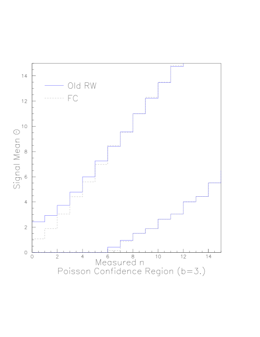
FIG. 1.: The 90% C.L. belt for a Poisson probability with $b=3$, using the old R-W procedure (solid line) and the Feldman-Cousins unified procedure (dashed line).

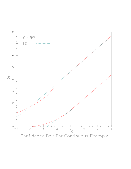
FIG. 2.: The 90% C.L. belt for the continuous probability example, using the old R-W procedure (solid line) and the Feldman-Cousins unified procedure (dashed line).

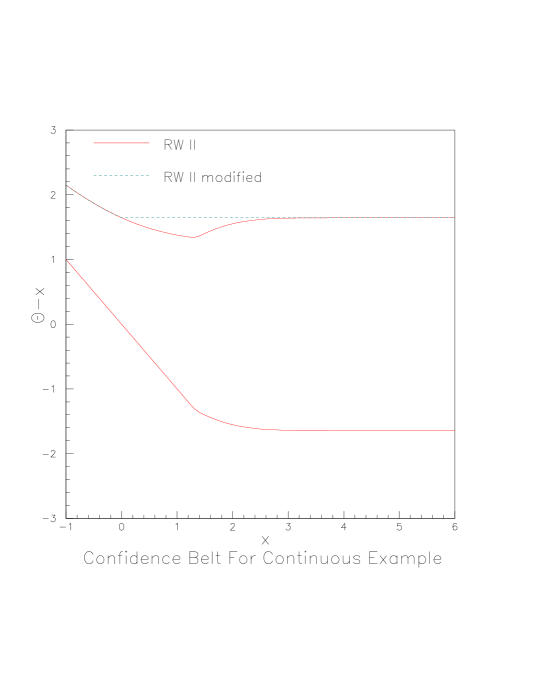
FIG. 3.: The 90% C.L. belt plotted as $\theta-x$ vs $x$ using the Bayesian procedure and a conservative modification (dashed) for the continuous example.

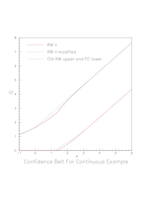
FIG. 4.: The 90% C.L. belt using the Bayesian procedure (solid line) and the conservative modification (dashed line) for the continuous example. The old R-W upper limit and the F-C unified method lower limit are shown as dotted lines.

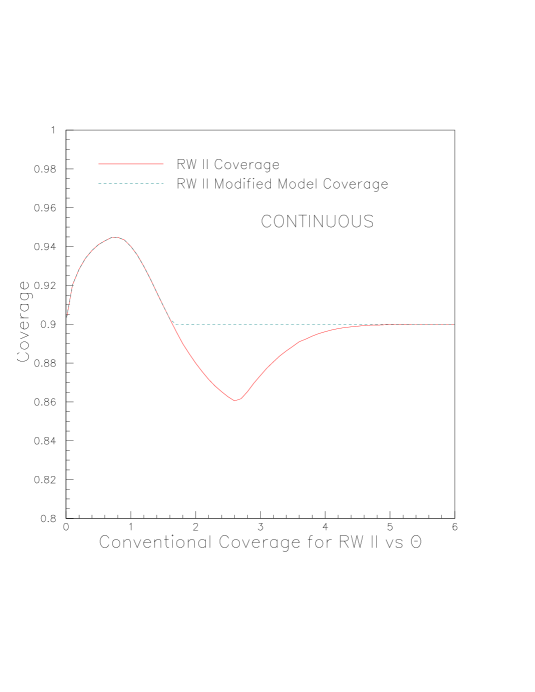
FIG. 5.: The conventional frequentist coverage for a Bayesian 90% C.L. belt for the Bayesian continuous model (solid line) and the conservative modification (dashed line).

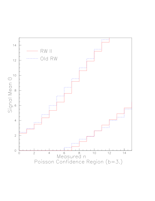
FIG. 6.: The 90% C.L. belt for the Poisson distribution with $b=3$ using the Bayesian procedure and the old R-W procedure (dashed line).

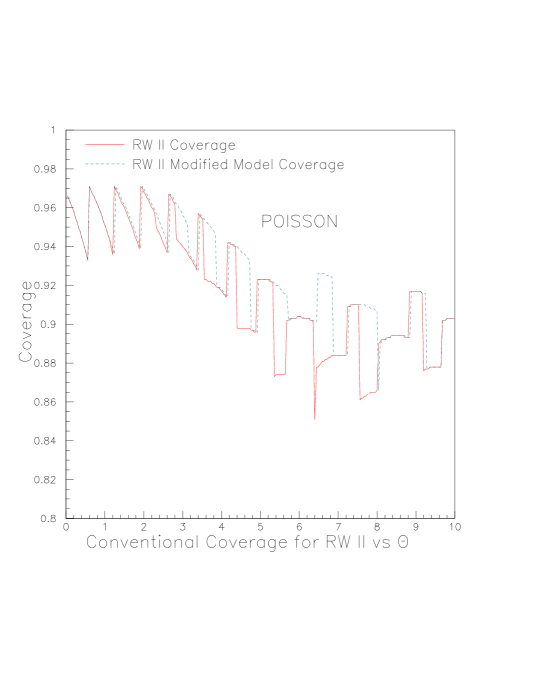
FIG. 7.: The conventional frequentist coverage obtained by this Bayesian procedure (solid line) and by the conservative modification (dashed line) for $b=3$.

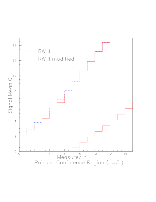
FIG. 8.: The 90% C.L. belt for the Poisson distribution with $b=3$ using the Bayesian procedure (solid line) and the conservative modification (dashed line).

REFERENCES

- [1] G.J. Feldman and R.D. Cousins, Unified approach to the classical statistical analysis of small signals, Phys. Rev. D57, 3873 (1998).
- [2] K. Eitel and B. Zeitnitz, The search for neutrino oscillations with KARMEN, in Neutrino Physics and Astrophysics, Procedings of the XVIII International Conference on Neutrino Physics and Astrophysics, Takayama, Japan, edited by Y. Suzuki and Y. Totsuka, North Holland (1999).
- [3] B.P. Roe and M.B. Woodroofe, Improved Probability Method for Estimating Signal in the Presence of Background, Phys. Rev. D 60, 053009 (1999).
- [4] Robert D. Cousins, Application of Conditioning to the Gaussian-with-Boundary Problem in the Unified Approach to Confidence Intervals, arXiv:physics/0001031, 15 Jan 2000, submitted to Phys. Rev., 2000.
- [5] A.P. Dempster, N.M. Laird, and D.B. Rubin, Maximum Likelihood from Incomplete Data via the EM Algorithm, Roy. Stat. Soc. B39, 1 (1977).
- [6] B.P. Roe, Probability and Statistics in Experimental Physics, Second Edition, Springer-Verlag, New York, to be published in 2001.
- [7] A.L. Read, Modified Frequentist Analysis of Search Results (The Method), Proceedings of the Workshop on Confidence Limits at CERN, January 17-18, 2000, to be issued as a CERN Yellow Report.
- [8] H. Wang and M. Woodroofe, to appear in Ann. Statist.
- [9] J. Pratt, J. Amer. Statist. Assn., 56 549-567,(1961).