Abstract

We present a measurement of the $W$ boson mass using data collected with the CDF detector during the 1994-95 collider run at the Fermilab Tevatron. A fit to the transverse mass spectrum of a sample of 30,115 $W\rightarrow\ e\nu$ events recorded in an integrated luminosity of 84 pb^-1 gives a mass $M_{W}={\rm 80.473\pm 0.065(stat.)\pm 0.092(syst.)}$ GeV/c². A fit to the transverse mass spectrum of a sample of 14,740 $W\rightarrow\ \mu\nu$ events from 80 pb^-1 gives a mass $M_{W}={\rm 80.465\pm 0.100(stat.)\pm 0.103(syst.)}$ GeV/c². The dominant contributions to the systematic uncertainties are the uncertainties in the electron energy scale and the muon momentum scale, 0.075 GeV/c² and 0.085 GeV/c², respectively. The combined value for the electron and muon channel is $M_{W}=80.470\pm 0.089$ GeV/c². When combined with previously published CDF measurements, we obtain $M_{W}=80.433\pm 0.079$ GeV/c².

I Introduction

This paper describes a measurement of the $W$ mass using $W$ boson decays observed in antiproton-proton ($\overline{p}p$) collisions produced at the Fermilab Tevatron with a center-of-mass energy of 1800 GeV. The results are from an analysis of the decays of the $W$ into a muon and neutrino in a data sample of integrated luminosity of 80 pb^-1, and the decays of the $W$ into an electron and neutrino in a data sample of 84 pb^-1, collected by the Collider Detector at Fermilab (CDF) from 1994 to 1995. This time period is referred to as Run IB whereas the period from 1992 and 1993 with about 20 pb^-1 of integrated luminosity is referred to as Run IA.

The relations among the masses and couplings of gauge bosons allow incisive tests of the Standard Model of the electroweak interactions [1]. These relations include higher-order radiative corrections which are sensitive to the top quark mass, $M_{\rm top}$, and the Higgs boson mass, $M_{\rm Higgs}$ [2]. The $W$ boson mass provides a significant test of the Standard Model in the context of measurements of the properties of the $Z$ boson, measurements of atomic transitions, muon decay, neutrino interactions, and searches for the Higgs boson.

Direct measurement of the $W$ mass originated at the antiproton-proton collider at CERN [3]. Measurements at the Fermilab Tevatron collider by CDF [4] and DO/ [5] have greatly improved precision. At LEP II, the $W$ boson mass has been measured from the $W$ pair production cross section near threshold [6] and by direct reconstruction of the two $W$s [7]. The average of direct measurements including the analysis in this paper is of $80.39\pm 0.06$ GeV/c² [8].

Indirect $W$ mass determinations involve $Z$ boson measurements at LEP and SLC [9], charged- and neutral-current neutrino interactions at Fermilab [10], and the top quark mass measurement at Fermilab [11]. A recent survey [9] gives a $W$ mass of $80.381\pm 0.026$ GeV/c² inferred from indirect measurements.

The paper is structured as follows. A description of the detector and an overview of the analysis are given in Section II. The calibration and alignment of the central tracking chamber, which provides the momentum scale, is described in Section III. Section III also describes muon identification and the measurement of the momentum resolution. Section IV describes electron identification, the calorimeter energy scale, and the measurement of the energy resolution. The effects of backgrounds are described in Section V. Section VI describes a Monte Carlo simulation of $W$ production and decay, and QED radiative corrections. Section VII describes the measurement of the detector response to the hadrons recoiling against the $W$ in the event, necessary to infer the neutrino momentum scale and resolution. The knowledge of the lepton and recoil responses is incorporated in the Monte Carlo simulation of $W$ production and decay. Section VIII gives a description of the fitting method used to extract the $W$ mass from a comparison of the data and the simulation. It also presents a global summary of the measured values and the experimental uncertainties. Finally, the measured $W$ mass is compared to previous measurements and current predictions.

II Overview

This section begins with a discussion of how the nature of $W$ boson production and decay motivates the strategy used to measure the $W$ mass. The aspects of the detector and triggers critical to the measurement are then described. A brief description of the data samples used for the calibrations and for the mass measurement follows. A summary of the analysis strategy and comparison of this analysis with our last analysis concludes the section.

A Nature of $W$ Events

The dominant mechanism for production of $W$ bosons in antiproton-proton collisions is antiquark-quark annihilation. The $W$ is produced with momentum relative to the center-of-mass of the antiproton-proton collision in the transverse ($x,y$) and longitudinal ($z$) directions (see Figure 1). The transverse component of the momentum is balanced by the transverse momentum of hadrons produced in association with the $W$, referred to as the “recoil”, as illustrated in Figure 2.

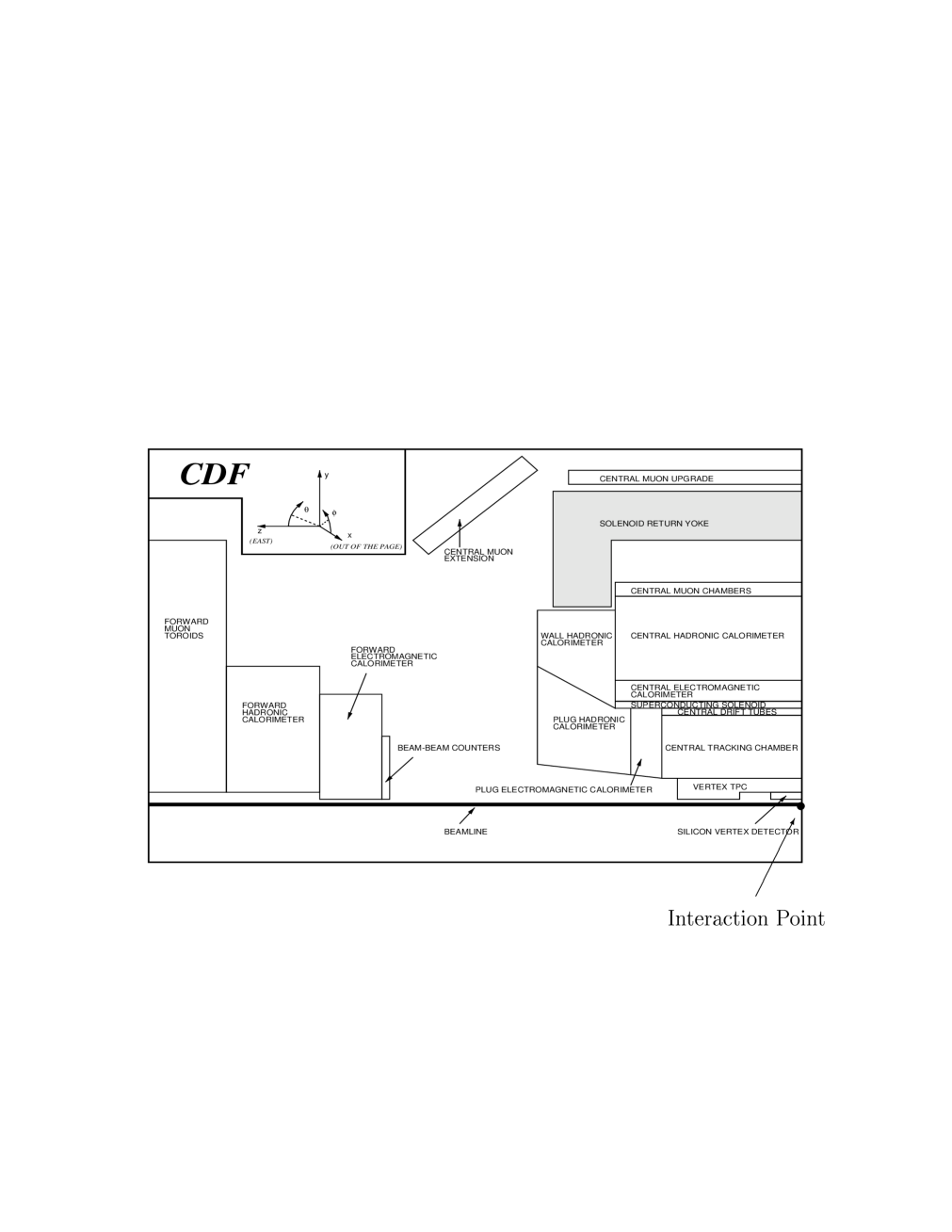
FIG. 1.: One quarter of the CDF detector. The detector is symmetric about the interaction point. CDF uses a cylindrical coordinate system with the $z$ (longitudinal) axis along the proton beam axis; $r$ is the transverse coordinate, and $\phi$ is the azimuthal angle. Pseudorapidity ($\eta$) is defined as $\eta\equiv-{\rm ln(tan}(\theta/2))$, where $\theta$ is the polar angle relative to the proton-beam direction.

FIG. 2.: Kinematics of $W$ boson production and decay for the events used in this analysis, as viewed in the plane transverse to the antiproton-proton beams. The recoil energy vector ${\bf u}$ is the sum of the transverse energy vectors $\bf E_{T}^{i}$ of the particles recoiling against the $W$. Although energy is a scalar quantity, “transverse energy” commonly denotes the transverse component of the vector whose $magnitude$ is the energy of the particle and $direction$ is parallel to the momentum of the particle.

The $W$ boson decays used in this analysis are the two-body leptonic decays producing an electron or muon and a neutrino. Since the apparatus neither detects the neutrino nor measures the $z$-component of the recoil momentum, much of which is carried in fragments of the initial proton and antiproton at small angles relative to the beams, there is insufficient information to reconstruct the invariant mass of the $W$ on an event-by-event basis. This analysis uses the transverse mass of each $W$ event, which is analogous to the invariant mass except that only the components transverse to the beamline are used. Specifically,

$$(M_{T}^{W})^{2}=(E_{T}^{\ell}+E_{T}^{\nu})^{2}-({\bf E}_{T}^{\ell}+{\bf E}_{T}^{\nu})^{2},$$ (1)

where $M_{T}^{W}$ is the transverse mass of the $W$, $E_{T}^{\ell}$ is the transverse energy (see Figure 2) of the electron or the transverse momentum of the muon, and $E_{T}^{\nu}$ is the transverse energy of the neutrino. The boldface denotes two-component vector quantities. The transverse energy of the neutrino is inferred from apparent energy imbalance in the calorimeters,

$${\raisebox{1.29167pt}{$\not$}{\bf E}_{T}}={\bf E}_{T}^{\nu}=-({\bf E}_{T}^{\ell}+{\bf u}),$$ (2)

where ${\bf u}$ denotes the transverse energy vector of the recoil (see Figure 2) measured by the calorimeters.

B Detector and Triggers

This section briefly describes those aspects of the CDF detector and triggers pertinent to the $W$ mass measurement. A more detailed detector description can be found in Reference [14]; recent detector upgrades are described in Reference [15] and references therein.

The CDF detector is an azimuthally and forward-backward symmetric magnetic detector designed to study $\overline{p}p$ collisions at the Tevatron. The magnetic spectrometer consists of tracking devices inside a 3-m diameter, 5-m long superconducting solenoidal magnet which operates at 1.4 T. The calorimeter is divided into a central region ($30^{\circ}<\theta<150^{\circ}$) outside the solenoidal magnet, end-plugs ($10^{\circ}<\theta<30^{\circ}$, $150^{\circ}<\theta<170^{\circ}$), which form the pole pieces for the solenoidal magnet, and forward and backward regions ($2^{\circ}<\theta<10^{\circ}$, $170^{\circ}<\theta<178^{\circ}$). Muon chambers are placed outside (at larger radius) of the hadronic calorimeters in the central region and behind added shielding. An elevation view of one quarter of the CDF detector is shown in Figure 1.

1 Tracking Detectors

A four-layer silicon microstrip vertex detector (SVX^′) [16] is used in this analysis to provide a precision measurement of the location of the beam axis (luminous region). The SVX^′ is located directly outside the 1.9-cm radius beryllium beampipe. The four layers of the SVX^′ are at radii of 2.9, 4.3, 5.7, and 7.9 cm from the beamline. Outside the SVX^′ is a set of vertex time projection chambers (VTX) [17], which provides $r$-$z$ tracking information out to a radius of 22 cm for $|\eta|<3.25$. The VTX is used in this analysis for finding the $z$ position of the antiproton-proton interaction (the event vertex). The event vertex is necessary for event selection, lepton track reconstruction, and the calculation of $E_{T}$.

Both the SVX^′ and VTX are mounted inside the central tracking chamber (CTC) [18], a 3.2-m long drift chamber that extends in radius from 31.0 cm to 132.5 cm. The CTC has 84 sampling wire layers, organized in 5 axial and 4 stereo “super-layers”. Axial super-layers have 12 radially separated layers of sense wires, parallel to the $z$ axis, that measure the $r$-$\phi$ position of a track. Stereo super-layers have 6 sense wire layers, with a $\sim\!2.5^{\circ}$ stereo angle, that measure a combination of $r$-$\phi$ and $z$ information. The stereo angle direction alternates at each stereo super-layer. Axial and stereo data are combined to form a 3-dimensional track. Details of the calibration and alignment of the CTC are given in Section III.

Track reconstruction uses $r$-$\phi$ information from the beam axis and the CTC axial layers, and $z$ information from the VTX $z$ vertex and the CTC stereo layers. In this analysis, the electron or muon momentum is measured from the curvature, azimuthal angle, and polar angle of the track as the particle traverses the magnetic field.

2 Calorimeters

The electromagnetic and hadronic calorimeters subtend 2$\pi$ in azimuth and from $-$4.2 to 4.2 in pseudorapidity ($\eta$). The calorimeters are constructed with a projective tower geometry, with towers subtending approximately 0.1 in pseudorapidity by 15^∘ in $\phi$ (central) or 5^∘ in $\phi$ (plug and forward). Each tower consists of an electromagnetic calorimeter followed by a hadronic calorimeter at larger radius. The energies of central electrons used in the mass measurement are measured from the electromagnetic shower produced in the central electromagnetic calorimeter (CEM) [19]. The central calorimeter is constructed as 24 “wedges” in $\phi$ for each half of the detector ($-1.1<\eta<0$ and $0<\eta<1.1$). Each wedge has 10 electromagnetic towers, which use lead as the absorber and scintillator as the active medium, for a total of 480 CEM towers. A proportional chamber (CES) measures the electron shower position in the $\phi$ and $z$ directions at a depth of $\sim 6$ radiation lengths in the CEM [19]. A fiducial region of uniform electromagnetic response is defined by avoiding the edges of the wedges. For the purposes of triggering and data sample selection, the CEM calibrations are derived from testbeam data taken during 1984-85; the tower gains were set in March 1994 using Cesium-137 gamma-ray sources. Details of the further calibration of the CEM are given in Section IV.

The calorimeters measure the energy flow of particles produced in association with the $W$. Outside the CEM is a similarly segmented hadronic calorimeter (CHA) [20]. Electromagnetic and hadronic calorimeters which use multi-wire proportional chambers as the active sampling medium extend this coverage to $|\eta|=4.2$ [21]. In this analysis, however, the recoil energy is calculated only in the region of full azimuthal symmetry, $|\eta|<3.6$. Understanding the response of these devices to the recoil from bosons is difficult from first principles as it depends on details of the flow and energy distributions of the recoil hadrons. The energy response to recoil energy is parameterized primarily using $Z\rightarrow\ e^{+}e^{-}$ and $Z\rightarrow\mu^{+}\mu^{-}$ events. Details of the calibration of the calorimeters to recoil energy are given in Section VII.

3 Muon Detectors

Four-layer drift chambers, embedded in the wedge directly outside (in radius) of the CHA, form the central muon detection system (CMU) [22]. The CMU covers the region $|\eta|<0.6$. Outside of these systems there is an additional absorber of 0.6 m of steel followed by a system of four-layer drift chambers (CMP). Approximately 84% of the solid angle for $|\eta|<0.6$ is covered by CMU, 63% by CMP, and 53% by both. Additional four-layer muon chambers (CMX) with partial (70 %) azimuthal coverage subtend $0.6<|\eta|<1$. Muons from $W$ decays are required in this analysis to produce a track (stub) in the CMU or CMX that matches a track in the CTC. The CMP is used in this measurement only in the Level 1 and Level 2 triggers. Details of the muon selection and reconstruction are given in Section III.

4 Trigger and Data Acquisition

The CDF trigger is a three-level system that selects events for recording to magnetic tape. The crossing rate of proton and antiproton bunches in the Tevatron is 286 kHz, with a mean interaction rate of 1.7 interactions per crossing at a luminosity of $\sim 1\times 10^{31}$ cm^-2 sec^-1, which is typical of the data presented here. The first two levels of the trigger [23] consist of dedicated electronics with data paths separate from the data acquisition system. The third level [24], which is initiated after the event information is digitized and stored, uses a farm of commercial computers to reconstruct events. The triggers selecting $W\rightarrow\ e\nu$ and $W\rightarrow\ \mu\nu$ events are described below.

At Level 1, electrons were selected by the presence of an electromagnetic trigger-tower with $E_{T}$ above 8 GeV (one trigger tower is two physical towers, which are longitudinally adjacent, adjacent in pseudorapidity). Muons were selected by the presence of a track stub in the CMU or CMX, and, where there is coverage, also in the CMP.

At Level 2, electrons from $W$ decay could satisfy one of several triggers. Some required a track to be found in the $r$-$\phi$ plane by a fast hardware processor [25] and matched to a calorimeter cluster; the most relevant required an electromagnetic cluster [23] with $E_{T}$ above 16 GeV and a track with $p_{T}$ above 12 GeV/c. This was complemented by a trigger which required an electromagnetic cluster with $E_{T}$ above 16 GeV matched with energy in the CES [26] and net missing transverse energy in the overall calorimeter of at least 20 GeV, with no track requirements. The muon Level 2 trigger required a track of at least 12 GeV/c that matches to a CMX stub (CMX triggers), both CMU and CMP stubs (CMUP triggers), or a CMU stub but no CMP stub (CMNP triggers). Due to bandwidth limitations, only about 43% of the CMX triggers and about 39% of the CMNP triggers were recorded.

At Level 3, reconstruction programs included three-dimensional track reconstruction. The muon triggers required a track with $p_{T}$ above 18 GeV/c matched with a muon stub. There were three relevant electron triggers. The first required an electromagnetic cluster with $E_{T}$ above 18 GeV matched to a track with $p_{T}$ above 13 GeV/c with requirements on track and shower maximum matching, little hadronic energy behind the cluster, and transverse profile in $z$ in both the towers and the CES. Because such requirements may create subtle biases, the second trigger required only a cluster above 22 GeV with a track above 13 GeV/c as well as 22 GeV net missing transverse energy in the overall calorimeter. The third trigger required an isolated 25 GeV cluster with no track requirement and with 25 GeV missing transverse energy.

Events that pass the Level 3 triggers were sorted and recorded. The integrated luminosity of the data sample is $\sim$80 pb^-1 in the muon sample and $\sim$84 pb^-1 in the electron sample.

C Data Samples

Nine data samples are employed in this analysis. These are described briefly below and in more detail in subsequent sections as they are used. A list of the samples follows:

• The $\psi\rightarrow\mu^{+}\mu^{-}$ sample. A sample of $\sim 500,000$ $\psi\rightarrow\mu^{+}\mu^{-}$ candidates with $2.7<M_{\mu^{+}\mu^{-}}<4.1$ GeV/c² is used to investigate the momentum scale determination and to understand systematic effects associated with track reconstruction.

• The $\Upsilon\rightarrow\mu^{+}\mu^{-}$ sample. A sample of $\sim 83,000$ $\Upsilon\rightarrow\mu^{+}\mu^{-}$ candidates with $8.6<M_{\mu^{+}\mu^{-}}<11.3$ GeV/c² offers checks of the momentum scale determination that are statistically weaker but systematically better than those from the $\psi\rightarrow\mu^{+}\mu^{-}$ sample.

• The $Z\rightarrow\mu^{+}\mu^{-}$ sample. A sample of $\sim$1,900 dimuon candidates near the $Z$ mass determines the momentum scale and resolution, and is used to model the response of the calorimeters to the recoil particles against the $Z$ and $W$ boson, and to derive the $Z$ and $W$ $p_{T}$ distributions in the $W\rightarrow\ \mu\nu$ analysis.

• The $W\rightarrow\mu\nu$ sample. A sample of $\sim 14,700$ $W\rightarrow\mu\nu$ candidates is used to measure the $W$ mass.

• The inclusive electron sample. A sample of $\sim$750,000 central electron candidates with $E_{T}>8$ GeV is used to calibrate the relative response of the central electromagnetic calorimeter (CEM) towers.

• The Run IA inclusive electron sample. A sample of $\sim$210,000 central electron candidates with $E_{T}>9$ GeV is used to measure the magnitude and the distribution of the material, in radiation lengths, between the interaction point and the CTC tracking volume.

• The $W\rightarrow e\nu$ sample. A sample of $\sim$30,100 $W\rightarrow e\nu$ candidates is used to align the CTC, to compare the CEM energy scale to the momentum scale, and to measure the $W$ mass.

• The $Z\rightarrow\ e^{+}e^{-}$ sample. A sample of $\sim$1,500 dielectron candidates near the $Z$ mass is used to determine the electron energy scale and resolution, to model the response of the calorimeters to the recoil particles against the $Z$ and $W$ boson, and to derive the $Z$ and $W$ $p_{T}$ distributions in the $W\rightarrow\ e\nu$ analysis.

• The minimum bias sample. A total of $\sim 2,000,000$ events triggered only on a coincidence of two luminosity counters is used to help understand underlying event.

D Strategy of the Analysis

The determination of the momentum and energy scales is crucial to the $W$ mass measurement. Momentum is the kinematic quantity measured for muons; for electrons, the energy measured in the calorimeter is the quantity of choice as it has better resolution and is much less sensitive than the momentum to the effects of bremsstrahlung [27]. The spectrometer measures the momentum $(p)$ of muons and electrons, and the calorimeter measures the energy $(E)$ of electrons. This configuration allows in situ calibrations of both the momentum and energy scales directly from the collider data. The final alignment of the CTC wires is done with high momentum electrons, exploiting the charge independence of the electromagnetic calorimeter measurement since both positives and negatives should give the same momentum for a given energy. The momentum scale of the magnetic spectrometer is then studied using the reconstructed mass of the $\psi\rightarrow\mu^{+}\mu^{-}$ and $\Upsilon\rightarrow\mu^{+}\mu^{-}$ resonances, exploiting the uniformity, stability, and linearity of the magnetic spectrometer. Similar studies for the calorimeter are done using the average calorimeter response to electrons (both $e^{+}$ and $e^{-}$) of a given momentum. The momenta of lepton tracks from $W$ decays reconstructed with the final CTC calibration typically change from the initial values used for data sample selection by less than 10%; their mean changes by less than 0.1%. The final CEM calibration differs from the initial source/testbeam calibration in early runs on average by less than 2%, with a gradual decline of $\sim$5% during the data-taking period. Fits to the reconstructed $Z\rightarrow\mu^{+}\mu^{-}$ and $Z\rightarrow\ e^{+}e^{-}$ masses, along with linearity studies, provide the final momentum and energy scales. The mass distributions are also used to determine the momentum and energy resolutions.

The detector response to the recoil ${\bf u}$ is calibrated primarily using $Z\rightarrow\mu^{+}\mu^{-}$ and $Z\rightarrow\ e^{+}e^{-}$ decays in the muon and electron analyses, respectively. These are input to fast Monte Carlo programs which combine the production model and detector simulation.

The observed transverse mass lineshape also depends on the transverse and longitudinal $W$ momentum spectra. The $p_{T}^{W}$ spectrum is derived from the $Z\rightarrow\ e^{+}e^{-}$ and $Z\rightarrow\mu^{+}\mu^{-}$ data and the theoretical calculations. The $p_{T}^{Z}$ spectrum is measured from the leptons in the $Z$ decays by taking into account the lepton momentum and energy resolution. The theoretical calculations are used to correct the difference between the $p_{T}^{Z}$ and $p_{T}^{W}$ distributions. The observed $\bf u$ distributions provide consistency checks. The longitudinal spectrum is constrained by restricting the choice of parton distribution functions (PDFs) to those consistent with data.

To extract the $W$ mass, the measured $W$ transverse mass spectrum is fit to fast Monte Carlo spectra generated at a range of $W$ masses. Electromagnetic radiative processes and backgrounds are included in the simulated lineshapes. The uncertainties associated with known systematic effects are estimated by varying the magnitude of these effects in the Monte Carlo simulation and refitting the data.

E Comparison with Run IA Analysis

This analysis is similar to that of our last (Run IA) measurement [4], with datasets $\sim 4.5$ times larger. The direct use of the $Z$ events in modeling $W$ production and recoil hadrons against the $W$ [4, 12] is replaced with a more sophisticated parameterization [28]. In this analysis our efforts to set a momentum scale using the $\psi$ and $\Upsilon$ dimuon masses and then to transfer that to an energy scale using $E/p$ for $W$ electrons did not produce a self-consistent picture, particularly the reconstructed mass of the $Z$ with electron pairs. Instead we choose to normalize the electron energy and muon momentum scales to the $Z$ mass, in order to minimize the systematic effects, at the cost of a modest increase in the overall scale uncertainty due to the limited $Z$ statistics. A discussion of this problem is given in Appendix A. The instantaneous luminosity of this dataset is a factor of $\sim$2 larger, resulting in higher probability of having additional interactions within the same beam crossing. Also, we have included muon triggers from a wider range of polar angle.

III Muon Measurement

In the muon channel, the $W$ transverse mass depends primarily on the muon momentum measurement in the central tracking chamber (CTC). This section begins with a description of the reconstruction of charged-particle trajectories and describes the CTC calibration and alignment. It then describes the selection criteria to identify muons and the criteria to select the $W\rightarrow\ \mu\nu$ and $Z\rightarrow\mu^{+}\mu^{-}$ candidates. The momentum scale is set by adjusting the measured mass from $Z\rightarrow\mu^{+}\mu^{-}$ decays to the world-average value of the $Z$ mass [29]. The muon momentum resolution is extracted from the width of the $Z\rightarrow\mu^{+}\mu^{-}$ peak in the same dataset. The muon momentum scale is checked by comparing the $\Upsilon$ and $\psi$ masses with the world-average values. Since the average muon momentum is higher in $Z$ decays than $W$ decays, a correction would be necessary for the $W$ mass determination if there were a momentum nonlinearity. Studies of the $Z$, $\Upsilon$, and $\psi$ mass measurements indicate that the size of the nonlinearity is negligible.

A Track Reconstruction

1 Helical Fit

The momentum of a charged particle is determined from its trajectory in the CTC. The CTC is operated in a nearly (to within $\sim\!$1%) uniform axial magnetic field. In a uniform field, charged particles follow a helical trajectory. This helix is parametrized by: curvature, $C$ (inverse diameter of the circle in $r$-$\phi$); impact parameter, $D_{0}$ (distance of closest approach to $r=0$); $\phi_{0}$ (azimuthal direction at the point of closest approach to $r=0$); $z_{0}$ (the $z$ position at the point of closest approach to $r=0$); and $\cot\theta$, where $\theta$ is the polar angle with respect to the proton direction. The helix parameters are determined taking into account the nonuniformities of the magnetic field using the magnetic field map. The magnetic field was measured by NMR probes at two reference points on the endplates of the CTC during the data-taking period as shown in Figure 3, and corrections are made on the magnetic field run-by-run to convert curvatures to momenta.

FIG. 3.: Variation of the average magnetic field as a function of run number. The left side of the plot corresponds to January 1994 and the right side of the plot to July 1995.

The momentum resolution is improved by a factor of $\sim$2 by constraining tracks to originate from the interaction point (“beam-constraint”). The $z$ location of the interaction point is determined using the VTX for each event with a precision of 1 mm. The distribution of these interaction points has an RMS spread of 25$-$30 cm, depending on accelerator conditions. The $r$-$\phi$ location of the beam axis is measured with the SVX^′, as a function of $z$, to a precision of 10 $\mu$m. The beam axis is tilted with respect to the CTC axis by a slope that is typically about 400 microns per meter.

2 Material Effects on Helix Parameters

The material between the interaction region and the CTC tracking volume leads to the helix parameters measured in the CTC that are different than those at the interaction point. For example, in traversing 7% of a radiation length, muons lose about 5 MeV on average due to $dE/dx$ energy loss, which is significant for low $p_{T}$ tracks. Because of its small mass, electrons passing through the material have a large amount of (external) bremsstrahlung which changes both the curvature and impact parameter of the electrons. The beam constraint fit accounts for the $dE/dx$, and restores some of the energy loss due to the external bremsstrahlung. In order to make accurate corrections for the $dE/dx$, and properly simulate biases from external bremsstrahlung, the magnitude and distribution of the material need to be understood.

The material distribution is measured using a Run IA sample of 210,000 photon conversions, where the conversion rate is proportional to the traversed depth in radiation lengths. Conversion candidates are selected from the 9 GeV inclusive electron sample. An electron associated with an oppositely-charged partner track close in $\theta$ and distance at the point of conversion (the point at which the two helices are parallel in azimuth) is identified as a $\gamma\rightarrow\mbox{$e^{+}e^{-}$}$ candidate. To optimize the resolution on the measured conversion location, a two-constraint fit is applied to the helix parameters of the two tracks: the separation is constrained to vanish, and the angle $\phi$ from the beam spot to the conversion point is constrained to match the $\phi$ of the photon momentum vector. These constraints give an average observed resolution of 0.41 cm on the conversion radius, to be compared with an expected resolution of 0.35 cm. The radial distributions for conversions and backgrounds up to the innermost superlayer in the CTC are shown in Figure 4. The prominent peak at 28 cm is due to the inner support structure of the CTC. Other structures such as the silicon layers of the SVX and the VTX walls can be clearly resolved. This resolution is important since we need to fix the proportionality constant between conversions and radiation lengths by calibrating on a feature of known composition. The CTC inner support is chosen for this purpose since its construction is well-documented. Its thickness at normal incidence is $(1.26\pm 0.06)$% of a radiation length. The result for the integrated material thickness before the CTC volume, averaged over the vertex distribution and angular distribution, is $(7.20\pm 0.38)$% of a radiation length . Variations in conversion-finding efficiency and electron trigger efficiency as a function of the conversion point are taken into account. Other choices for the “standard radiator” such as the wires of the innermost superlayer in the CTC, as shown in Figure 5, give consistent results.

FIG. 4.: The radial (R) distributions for conversions (solid line) and background (dashed line) for the Run IA inclusive electron sample. R is negative when the photon momentum direction is opposite to the vector from the beam spot to the conversion position due to the detector resolution.

FIG. 5.: Reconstructed photon conversion vertex density in the $r-\phi$ plane for the innermost superlayer in the CTC, folded into 1/30 of the circumference (this layer has 30-fold symmetry). Each point represents one reconstructed vertex.

Another check is provided by the $E/p$ distribution of electrons from $W$ decay (see Figure 6), where $E$ is the electron energy measured by the CEM and $p$ is the electron momentum measured by the CTC. External bremsstrahlung photons [30] are collinear with the electron track at emission and typically point at the calorimeter tower struck by the electron track so that the calorimeter collects the full energy. Since the track momentum is reduced by the radiated energy, the $E/p$ distribution develops a high-side tail. Final state radiation from electron production (internal bremsstrahlung) is about a 20 % contribution to this tail. We define the fraction of events in the tail, $f_{tail}$, to be the fraction of events in the region $1.4<E/p<1.8$. The lower bound is far enough away from the peak to be insensitive to resolution effects. After a small QCD background correction, we find :

$$f_{tail}=0.0488\pm 0.0014({\rm stat.})\pm 0.0004({\rm syst.}).$$

The Monte Carlo simulation, including internal radiative effects, reproduces this value when the material equals $(7.55\pm 0.37)$% of a radiation length, in good agreement with the value from conversion photons above.

An appropriate material distribution is applied to muon and electron tracks on a track-by-track basis.

FIG. 6.: $E/p$ distribution of electrons in the $W\rightarrow\ e\nu$ sample. The histogram indicates the simulation.

B CTC Calibration and Alignment

The CTC calibration and alignment proceeds in two steps. First, the relationship between the measured drift time and the distance to the sense wire is established. Second, the relative alignment of wires and layers in the CTC is performed. Small misalignments left after these procedures are removed with parametric corrections.

1 Time-to-distance calibration

Electronic pulsing, performed periodically during the data-taking period, gives relative time pedestals for each sense wire. Variations in drift properties for each super-layer are removed run-by-run. Additional corrections for nonuniformity in the drift trajectories are made based on data from many runs. After the calibration and alignment described in Section III B 2, the CTC drift-distance resolution is determined to be 155 $\mu$m (outer layers) to 215 $\mu$m (inner layers), to be compared with $\sim 120$ $\mu$m expected from diffusion alone, and $\sim 200$ $\mu$m expected from test-chamber results.

2 Wire and layer alignment

The initial individual wire positions are taken to be the nominal positions determined during the CTC construction [18]. The distribution of differences between these nominal positions and the positions determined with an optical survey has an RMS of 25 $\mu$m. The 84 layers of sense wires are azimuthally aligned relative to each other by requiring the ratio of energy to momentum $E/p$ for electrons to be independent of charge. A physical model for these misalignments is a coherent twist of each endplate as a function of radius. A sample of about $40,000$ electrons with $0.8<E/p<1.2$ from the $W\rightarrow e\nu$ sample (see Figure 6) is used for the alignment. The alignment consists of rotating each entire layer on each end of the CTC by a different amount $r\times\Delta\phi$ with respect to the outermost superlayer (superlayer 8) where the relative rotation of two endplates is expected to be the smallest according to the chamber construction. The stereo alignment is adjusted to account for the calculated endplate deflection due to wire tension. The measured deviation of each layer from its nominal position after this alignment is shown in Figure 7.

FIG. 7.: The deviation ($r\times\Delta\phi$) of each CTC layer from its nominal position at the end plates ($|z|$ = 150 cm) in cm, versus the layer number. The solid (open) circles represent the west (east) CTC endplate.

Figure 8 demonstrates the elimination of misalignment after the alignment (open circles). A small residual dependence of the $J/\psi$ mass on cot$\theta$ remains, which is removed with the correction,

$${\rm cot}\theta\rightarrow 1.0004\times{\rm cot}\theta.$$ (3)

The only significant remaining misalignments are an azimuthally($\phi$)-modulated charge difference in $<E/p>$ and a misalignment between the magnetic field direction and the axial direction of the CTC. The $\phi$ modulation is removed with the correction

$$C\rightarrow C-0.00031\times\mbox{sin}~{}(\phi_{0}\ -\ 3.0)$$ (4)

where $C$ equals to $Q\times 1/p_{T}$ (GeV/c)^-1, $Q$ is the charge of the lepton, the coefficient corresponds to a nominal beam position displacement of 37 $\mu$m, and $\phi$ is in radians. The magnetic field misalignment is removed with the correction

$$|C|\rightarrow|C|\cdot(1-0.0017\cdot{\rm cot}\theta\cdot{\rm sin}(\phi_{0}-1.9)).$$ (5)

FIG. 8.: Measured $J/\psi$ mass relative to the overall final mass measurement as a function of $\Delta$cot$\theta$ = cot$\theta_{\mu^{+}}$ $-$ cot$\theta_{\mu^{-}}$. The solid triangles and open circles are before and after the Run IB calibration and alignment, respectively. Solid circles show the distribution with the cot$\theta$ correction of 1.0004$\times$cot$\theta$.

C Muon Identification

The $W$ mass analysis uses muons traversing the central muon system (CMU) and the central muon extension system (CMX).

The CMU covers the region $|\eta|~{}<0.6$. The CMX extends the coverage to $|\eta|~{}<1$. There are approximately five to eight hadronic absorption lengths of material between the CTC and the muon chambers. Muon tracks are reconstructed using the drift chamber time-to-distance relationship in the transverse ($\phi$) direction, and charge division in the longitudinal ($z$) direction. Resolutions of 250 $\mu$m in the drift direction and 1.2 mm in $z$ are determined from cosmic-ray studies [22]. Track segments consisting of hits in at least three layers are found separately in the $r$-$\phi$ and $r$-$z$ planes. These two sets of segments are merged and a linear fit is performed to generate three-dimensional track segments (“stubs”). Figure 9 shows the effects of the bandwidth limitation of the CMX and CMNP triggers (see Section II B 4) and partial azimuthal coverage (see Section II B 3).

FIG. 9.: The $\eta$ and $\phi$ distributions of muons are shown in (a) and (b) for $W$ decays, and (c) and (d) for $Z$ decays. Points (histograms) show the data (the simulation) with statistical uncertainties.

Muons from $W$, $Z$, $\Upsilon$, and $\psi$ decays are identified in the following manner. The muon track is extrapolated to the muon chambers through the electromagnetic and hadronic calorimeters. The extrapolation must match to a track segment in the CMU or CMX. For high $p_{T}$ muons from $W$ or $Z$ decays, the $r\times\Delta\phi$ matching is required to be within 2 cm; the RMS spread of the matching is 0.5 cm. For low $p_{T}$ muons from $\Upsilon$ and $\psi$ decays, a $p_{T}$ dependent matching is required to allow for multiple scattering effects. Since the energy in the CEM tower(s) traversed by the muon is 0.3 GeV on average, the CEM energy is required to be less than 2 GeV for $W$ and $Z$ muons. This cut is not applied to muons from $\Upsilon$ or $\psi$ decays since $\Upsilon$’s and $\psi$’s are often produced with particles associated with the same initial partons. Since the energy in the CHA tower(s) traversed by the muon is 2 GeV on average, the CHA energy is required to be less than 6 GeV. In order to remove events with badly measured tracks, muon tracks are required to pass through all nine superlayers of the CTC, and to have the number of CTC stereo hits greater than or equal to 12. Muon tracks in the $W\rightarrow\ \mu\nu$ and $Z\rightarrow\mu^{+}\mu^{-}$ data samples must satisfy $|D_{0}|<$ 0.2 cm, where $D_{0}$ is the impact parameter in the $r$-$\phi$ plane of the muon track with respect to the beam spot. This reduces backgrounds from cosmic rays and QCD dijet events. Additional cosmic ray background events are removed from the $W\rightarrow\ \mu\nu$ and $Z\rightarrow\mu^{+}\mu^{-}$ samples when the hits of the muon track and the hits on the opposite side of the beam pipe, back-to-back in $\phi$, can be fit as one continuous trojectory.

D Event Selection: $W\rightarrow\ \mu\nu$; $Z,\Upsilon,\psi\rightarrow\mu^{+}\mu^{-}$

1 $W\rightarrow\mu\nu$ and $Z\rightarrow\mu^{+}\mu^{-}$ event selection

The event selection criteria for the $W\rightarrow\mu\nu$ mass measurement are intended to produce a sample with low background and with well-understood muon and neutrino kinematics. These criteria yield a sample that can be accurately modeled by simulation, and also preferentially choose those events with a good resolution for the transverse mass. The $Z$ sample is used to calibrate the muon momentum scale and resolution, to model the energy recoiling against the $Z$ and $W$, and to derive the $Z$ and $W$ transverse momentum spectra ($p_{T}^{Z}$ and $p_{T}^{W}$). In order to minimize biases in these measurements, the $Z\rightarrow\mu^{+}\mu^{-}$ event selection is chosen to be as similar as possible to the $W\rightarrow\ \mu\nu$ event selection.

Both $W\rightarrow\ \mu\nu$ and $Z\rightarrow\mu^{+}\mu^{-}$ sample extractions begin with events that pass a Level 3 high-$p_{T}$ muon trigger as discussed in Section 2. From these, a final sample is selected with the criteria listed in Table I and described in detail below. The event vertex chosen is the one reconstructed by the VTX closest in $z$ to the origin of the muon track, and it is required to be within 60 cm in $z$ of the origin of the detector coordinates. For the $Z$ sample, the two muons are required to be associated either with the same vertex or with vertices within 5 cm of each other. For the $W$ sample, in order to reduce backgrounds from $Z\rightarrow\mu^{+}\mu^{-}$ and cosmic rays, events containing any oppositely charged track with $p_{T}>$ 10 GeV/c and $M_{\mu,track}>50$ GeV/c² are rejected. Candidate $W\rightarrow\ \mu\nu$ events are required to have a muon CTC track with $p_{T}>$ 25 GeV/c and a neutrino transverse energy $E_{T}^{\nu}>$ 25 GeV. A limit on recoil energy of ${|\bf u|}<20$ GeV reduces QCD background and improves transverse mass resolution. Candidate $Z\rightarrow\mu^{+}\mu^{-}$ events are required to have two muons with $p_{T}>25$ GeV/c. The two muon tracks must be oppositely charged. This requirement removes no events, indicating that the background in the $Z$ sample is negligible. The transverse mass in the region $65<M_{T}<100$ GeV/c² and the mass in the region $80<M<100$ GeV/c² are used for extracting the $W$ mass and the $Z$ mass, respectively. These mass cuts apply only for mass fits and are absent when we otherwise refer to the $W$ or $Z$ sample. The final $W$ sample contains 23,367 events, of which 14,740 events are in the region 65 $<M_{T}<$ 100 GeV/c². The final $Z$ sample contains 1,840 events which are used for modeling the recoil energy against the $W$ and for deriving $p_{T}^{W}$, of which 1,697 events are in the region $80<M<100$ GeV/c².

Criterion	W events after cut	Z events after cut
Initial sample with $Z$ vertex requirement	60,607	4,787
$E_{T}^{\rm CEM}<2$ GeV	56,489	3,349
Not a cosmic candidate	42,296	2,906
Impact parameter $|D_{0}|<0.2$ cm	37,310	2,952
Track - muon stub match	36,596	2,752
Stereo hits $\geq$ 12	34,062	2,442
Tracks through all CTC superlayers	33,887	1,991
$p_{T}>$ 25 GeV/c	28,452	1,966
$E_{T}^{\nu}>$ 25 GeV	24,881	N/A
$|\bf u|<$ 20 GeV	23,367	N/A
$p_{T}^{\mu\mu}<45$ GeV/c, $70<M^{\mu\mu}<110$ GeV/c2	N/A	1,840
Mass fit region	14,740	1,697

TABLE I.: Criteria used to select the $W\rightarrow\ \mu\nu$ and $Z\rightarrow\mu^{+}\mu^{-}$ samples.

2 $\Upsilon,\psi\rightarrow\mbox{$\mu^{+}\mu^{-}$}$ event selection

Samples of $\Upsilon$(1S, 2S, 3S) $\rightarrow\mbox{$\mu^{+}\mu^{-}$}$ events and $\psi$(1S, 2S) $\rightarrow\mbox{$\mu^{+}\mu^{-}$}$ events are used to check the momentum scale determined by $Z\rightarrow\mbox{$\mu^{+}\mu^{-}$}$ events. The sample extraction begins with events that pass a Level 2 and 3 dimuon trigger with muon $p_{T}>2$ GeV/c. The requirement on the event vertex is identical to that for the $Z\rightarrow\mu^{+}\mu^{-}$ selection. Both muons are required to have opposite charges.

Sample	# of events
$\Upsilon$(1S)	12,800
$\Upsilon$(2S)	3,500
$\Upsilon$(3S)	1,700
$J/\psi$	228,900
$\psi$(2S)	7,600

TABLE II.: The number of events in the $\Upsilon$ and $\psi$ samples after background subtraction.

Backgrounds are estimated from the dimuon invariant mass distributions in the sidebands (regions outside the mass peaks). The numbers of $\Upsilon$ and $\psi$ events after background subtraction are listed in Table II. The average $p_{T}$ of muons in the $\Upsilon$ sample is 5.3 GeV/c, and that in the $\psi$ sample is 3.5 GeV/c. The distributions of muon $p_{T}$ and the opening angle between the two muons in $\phi$ are shown in Figure 10. For comparison, the average $p_{T}$ of the muons and the average opening angle in the $Z$ sample are 43 GeV/c and 165^∘, respectively.

FIG. 10.: (a) Transverse momentum distributions of muons and (b) opening angle distributions between $\mu^{+}$ and $\mu^{-}$ in the $\Upsilon$(1S) and $J/\psi$ samples. The histograms are normalized to unit area.

E Event Selection Bias on $M_{W}$

The $W\rightarrow\ \mu\nu$ selection requires muons at all three trigger levels. Of these, only the level-2 trigger has a significant dependence on the kinematics of the muon; its efficiency varies by $\sim$5% with $\eta$ of the tracks. This variation, however, leads to a negligible variation ($\sim$2 MeV/c²) on the $W$ mass since the $M_{T}$ distribution is approximately invariant under $p_{Z}$ boosts. The $W$ mass would be more sensitive to the $p_{T}$ dependence of the inefficiency since $M_{T}$ is directly related to $p_{T}$. No $p_{T}$ dependence is seen, but the statistical limitation on measuring such a dependence leads to a 15 MeV/c² uncertainty on the $W\rightarrow\ \mu\nu$ mass.

The muon identification requirements may also introduce a bias on the $W$ mass. For example, if the $W$ decays such that the muon travels close to the recoil, there is greater opportunity for the recoil particles to cause the muon identification to fail. These biases are investigated by tightening the muon identification requirements and measuring the subsequent shifts in $M_{W}$. The maximum shift observed of 10 MeV/c² is taken as a systematic uncertainty.

F Momentum Scale and Resolution

A sample of $Z\rightarrow\mu^{+}\mu^{-}$ events is used to determine the momentum scale by normalizing the reconstructed $Z\rightarrow\mbox{$\mu^{+}\mu^{-}$}$ mass to the world-average mass [29], and to measure the momentum resolution in the high-$p_{T}$ region. Since the muon tracks from $Z$ decays have curvatures comparable to those for the $W$ mass determination, the systematic uncertainty from extrapolating the momentum scale from the $Z$ mass to the $W$ mass is small. The measurement is limited by the finite statistics in the $Z$ peak.

The $Z\rightarrow\mu^{+}\mu^{-}$ Monte Carlo events are generated at various values of $Z$ mass with the $Z$ width fixed to the world average [29]. The generation program includes the $\gamma\rightarrow\mbox{$\mu^{+}\mu^{-}$}$ events and QED radiative effects, $Z\rightarrow\mu\mu\gamma$ [31, 32], but uses a QCD leading order calculation so that the $Z$ is generated at $p_{T}^{Z}=0$. The $Z$ is then given a transverse momentum whose spectrum is extracted from the $Z\rightarrow\mu^{+}\mu^{-}$ data (see Section VI). The generated muons are reconstructed by the detector simulation where CTC wire hit patterns, measured from the real $W\rightarrow\ e\nu$ data, are used to determine a covariance matrix of the muon track, and the track parameters are smeared according to this matrix. A beam constraint is then performed with the identical procedure as is used for the real data. The final covariance error matrix is scaled up by a free parameter to make the beam constraint momentum resolution agree with the data. The detector acceptance is modeled according to the nominal geometry. The simulation includes the effects of the bandwidth limitation of the CMX triggers. Figure 9 illustrates how well the effects of the acceptance and the bandwidth limitation are simulated. The mass distribution of the $Z\rightarrow\mu^{+}\mu^{-}$ data, shown in Figure 11, is then fit to simulated lineshapes, where the input $Z$ mass and the scale parameter to the covariance matrix (or the momentum resolution) are allowed to vary.

FIG. 11.: Results of fit to $Z$ mass and momentum resolution. (a) Invariant mass distribution. The points are the data, and the solid line is the Monte Carlo simulation (normalized to the data) with best fit. (b) Correlation between the scale factor and the momentum resolution.

Fitting the invariant mass distribution in the region $80<M_{\mu\mu}<100$ GeV/c² with a fixed $\Gamma_{Z}$ [29] yields

$$M_{Z}=\rm 91.110\pm 0.097(stat.)\pm 0.020(syst.)~{}GeV/c^{2},$$ (6)

and momentum resolution

$$\delta(1/p_{T})=(0.091\pm 0.004(\rm stat.))\times 10^{-2}~{}\mbox{(GeV/c)${}^{-1}$.}$$ (7)

Equation 6 results in the momentum scale factor

$${M_{Z}^{\rm PDG}\over M_{Z}^{\rm CDF}}=1.00085\pm 0.00106$$ (8)

which is applied to momenta of muons and electrons. The fit is shown in Figure 11. The two parameters, $\delta(1/p_{T})$ and $M_{Z}^{\rm PDG}/M_{Z}^{\rm CDF}$, are largely uncorrelated, as shown.

Table III contains a list of the systematic uncertainties on the $Z$ mass. The largest uncertainty is from the radiative effects due to using the incomplete theoretical calculation [31]; the calculation includes the final state radiation only and has a maximum of one radiated photon. The effect arising from the missing diagrams is evaluated by using the PHOTOS package [33] which allows two photon emissions, and by using the calculation by U. Baur et al. [34] who have recently developed a complete $O(\alpha)$ Monte Carlo program which incorporates the initial state QED radiation from the quark-lines and the interference of the initial and final state radiation, and includes a correct treatment of the final state soft and virtual photonic corrections. When the PHOTOS package is used in the simulation instead, the change in the $Z$ mass is less than 10 MeV/c². The effect of the initial state radiation and the initial and final state interference is estimated to be 10 MeV/c² [34]. To be conservative these changes are added linearly and 20 MeV/c² is thus included in the systematic uncertainty. The choice of parton distribution functions and that of the $p_{T}^{Z}$ spectrum contribute negligible uncertainties.

A number of checks are performed to ensure that these results are robust and unbiased. The masses and resolutions at low and high $\eta$ are measured to be consistent. The resolution is cross-checked using the $E/p$ distribution in $W\rightarrow e\nu$ events, which is sensitive to the combined $E$ and $p$ resolution (see Section IV F and Figure 19). Consistent results are found when much simpler techniques are used, that is, comparing the mean $M_{Z}$, in the interval 86 – 96 GeV/c², between the data and the Monte Carlo simulation or fitting the invariant mass distribution with a Gaussian distribution. To address mis-measured tracks, a second Gaussian term is added to smear track parameters for 8% of the Monte Carlo events. The change in $M_{Z}$ is negligible.

Effect	Uncertainty on $M_{Z}^{\mu}$ (MeV/c2)
Statistics	97
Radiative corrections	20
Fitting	negligible
Parton distribution functions	negligible
$p_{T}^{Z}$ spectrum	negligible
Detector acceptance, triggers	negligible
Total	100

TABLE III.: Summary of uncertainties in measuring the $Z$ mass.

G Checks of Momentum Scale

The momentum scale is checked using $\psi$ and $\Upsilon$ masses, extracted by fitting the dimuon invariant mass distributions to simulated lineshapes which include QED radiative processes and backgrounds as shown in Figure 12. The muon momenta are corrected by the momentum scale factor shown in Eq. 8. The measured masses are summarized in Table 3.4. Table 3.5 compares the measured masses with the world-average values. Within the momentum scale uncertainty, the agreement is very good.

Resonance	Mass (MeV/c2)
$\Upsilon$(1S)	${\rm 9464.3\pm 0.7(stat.)\pm 1.6(syst.)\pm 10.1(scale)}$
$\Upsilon$(2S)	${\rm 10028.1\pm 2.1(stat.)\pm 1.6(syst.)\pm 10.7(scale)}$
$\Upsilon$(3S)	${\rm 10358.9\pm 3.6(stat.)\pm 1.6(syst.)\pm 11.0(scale)}$
$J/\psi$	${\rm 3098.4\pm 0.1(stat.)\pm 1.1(syst.)\pm 3.3(scale)}$
$\psi$(2S)	${\rm 3687.6\pm 0.5(stat.)\pm 1.1(syst.)\pm 3.9(scale)}$

TABLE IV.: Measured masses of the $\Upsilon$ and $\psi$ resonances with the momentum scale correction.

Resonance	World-Average Mass $M^{\rm PDG}$ (MeV/c2)	$M^{\rm CDF}/M^{\rm PDG}$  $-$  1 (%)
$\Upsilon$(1S)	$9460.4\pm 0.2$	$0.041\pm 0.018\pm 0.106$
$\Upsilon$(2S)	$10023.30\pm 0.31$	$0.048\pm 0.026\pm 0.106$
$\Upsilon$(3S)	$10355.3\pm 0.5$	$0.035\pm 0.038\pm 0.106$
$J/\psi$	$3096.88\pm 0.04$	$0.050\pm 0.035\pm 0.106$
$\psi$(2S)	$3686.00\pm 0.09$	$0.042\pm 0.033\pm 0.106$

TABLE V.: Measured masses of the $\Upsilon$ and $\psi$ resonances with the momentum scale correction are compared to the world averages. The second uncertainty in the last column is the momentum scale uncertainty, and the first uncertainty includes the statistical and the other systematic uncertainties.

FIG. 12.: The measured dimuon mass spectra near the (a) $\Upsilon$ masses, (b) $J/\psi$ mass, and (c) $\psi$(2S) mass. The curves are the best fits of lineshapes from the Monte Carlo simulation.

Source of Uncertainty	Uncertainty on $M_{\Upsilon}$ (MeV/c2)	Uncertainty on $M_{\psi}$ (MeV/c2)
Muon energy loss	1.5	1.0
Kinematics	0.4	0.1
Momentum Resolution	0.3	0.1
Non-Prompt Production	-	0.3
Misalignment	0.2	0.1
Background	0.1	0.1
Time variation	-	-
QED Radiative Effects	0.4	0.2
Fitting Procedure, Window	-	-
Total	1.6	1.1

TABLE VI.: Systematic uncertainties in $\Upsilon$ and $\psi$ mass measurements.

A list of the systematic uncertainties on the $\psi$ and $\Upsilon$ masses is given in Table VI. The entries in the table are described below.

Muon Energy Loss: The momentum of each muon is corrected for energy loss in the material traversed by the muon as described in Section III A 2. Uncertainties in the energy loss come from uncertainty in the total radiation length measurement and in material type. The measured $\Upsilon$ and $\psi$ masses vary by 0.8 MeV/c² and 0.3 MeV/c², respectively, when the average radiation length is changed by its uncertainty. Uncertainty due to material type is estimated to be 0.6 MeV/c² per muon track. This leads to 1.1 MeV/c² uncertainty in the $\Upsilon$ mass and 0.5 MeV/c² uncertainty in the $\psi$ mass. There is a 0.8 MeV/c² variation in the observed $\psi$ mass, which is not understood, when the mass is plotted as a function of the radiation length traversed. No statistically significant dependence ($<$ 0.7 MeV/c²) on the total radiation length is observed in the $\Upsilon$ mass. These variations of 0.7 MeV/c² in $M_{\Upsilon}$ and 0.8 MeV/c² in $M_{\psi}$ are taken as systematic uncertainties. Adding the uncertainties described above in quadrature, the total uncertainty is 1.5 MeV/c² in $M_{\Upsilon}$ and 1.0 MeV/c² in $M_{\psi}$.

Kinematics: Variation of the $p_{T}^{\Upsilon}$ and $p_{T}^{\psi}$ distributions allowed by the data and $p_{T}^{\mu}$ cuts results in uncertainties of 0.4 MeV/c² and 0.1 MeV/c² in $M_{\Upsilon}$ and $M_{\psi}$, respectively.

Momentum Resolution: Variation of the momentum resolution allowed by the data results in uncertainties of 0.3 MeV/c² and 0.1 MeV/c² in $M_{\Upsilon}$ and $M_{\psi}$, respectively.

Non-Prompt Production: About 20% of $\psi$’s come from decays of $B$ mesons, which decay at some distance from the primary vertex. The measured $\psi$ peak may be shifted by the application of the beam constraint. The difference in the $\psi$ mass between a fit using the beam constraint and a fit using a constraint that the two muons originate from the same vertex point is 0.3 MeV/c². This difference is taken as an uncertainty.

Misalignment: The CTC alignment eliminates most of the effects. The residual effects are measured by $\psi$ and $W$ samples and are removed by corrections as described in Section III B. The corrections and corresponding mass shifts on $M_{\Upsilon}$ are summarized in Table VII. The overall effects of 0.17 MeV/c² in $M_{\Upsilon}$ and less than 0.1 MeV/c² in $M_{\psi}$ are taken as a systematic uncertainty.

Source	Correction Formula	$\Delta M_{\Upsilon}$ (MeV/c2)
B-field direction	$|C|\rightarrow|C|\cdot(1-0.0017\cdot{\rm cot}\theta\cdot{\rm sin}(\phi_{0}-1.9))$	$+0.01$
$\phi_{0}$ dependence	$C\rightarrow C-0.00031\cdot{\rm sin}(\phi_{0}-3.0)$	$-0.24$
cot$\theta$ dependence	${\rm cot}\theta\rightarrow 1.0004\cdot{\rm cot}\theta$	$+0.40$
Total correction		$+0.17$

TABLE VII.: Systematic uncertainties in $\Upsilon$ and $\psi$ mass measurements.

Background: The backgrounds in the $\Upsilon$ and $\psi$ mass peak regions are estimated by fitting the invariant mass distributions in the sideband regions (regions away from the peaks) with quadratic, linear and exponential distributions. The backgrounds are included in the templates used to fit the masses. By varying the background shape, $M_{\psi}$ changes by less than 0.1 MeV/c² and $M_{\Upsilon}$ changes by 0.1 MeV/c².

Time Variation: As shown in Figure 13, there is no indication of a time variation in the measured mass over the data-taking period, even though the resolution worsens due to high occupancy in the CTC at high instantaneous luminosity during the latter portion of the data-taking period.

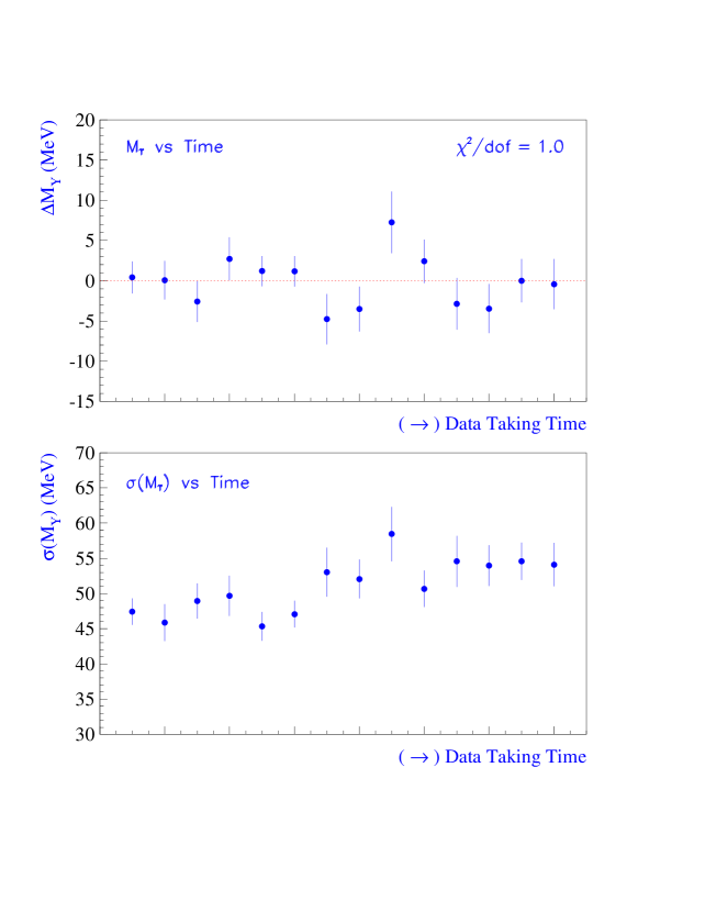
FIG. 13.: Variation of the measured $\Upsilon$(1S) mass (Top) and width (Bottom) as a function of time. The left side of the plot corresponds to January 1994 and the right side of the plot to July 1995. $\Delta M_{\Upsilon}$ is difference between the measured mass for a given time period and the mass using all the data.

QED Radiative Effects: The Monte Carlo program includes final state QED radiation from muons. The systematic uncertainties of 0.4 MeV/c² in $M_{\Upsilon}$ and 0.2 MeV/c² in $M_{\psi}$ represent missing diagrams such as two photon emission and the interference between the initial and final state radiation.

Fitting Procedure, Window: Consistent results are found when fitting windows are varied or much simpler fitting techniques are used, that is, comparing the mean $M_{\Upsilon}$ and $M_{\psi}$ and comparing the fit results with Gaussian plus linear distributions between the data and the Monte Carlo simulation.

H Momentum Nonlinearity

The average $p_{T}$ for $Z$ decay muons is about 4.5 GeV/c higher than that for $W$ decay muons. Since the momentum is calibrated with the $Z$ mass, any nonlinearity in the momentum measurement would translate into an incorrect momentum scale for the $W$ mass measurement. The momentum nonlinearity is studied using measured masses from a wide range of curvatures — the CTC does not directly measure momentum, but curvature, which is proportional to $1/p_{T}$. The curvature ranges from 0.1 to 0.5 (GeV/c)^-1 in the $J/\psi$ data, from 0.1 to 0.3 (GeV/c)^-1 in the $\Upsilon$(1S) data, and 0.02 to 0.04 (GeV/c)^-1 in the $Z$ data. Figure 14 shows the ratio of the measured mass to the world-average value as a function of the average curvature of two muons from these data. The ratios are flat and all are well within statistical uncertainty of the ratio from the $Z$ data. Since the curvature difference 0.003 (GeV/c)^-1 between the $W$ and $Z$ muons is much smaller than the range of curvature available in the $\psi$, $\Upsilon$, and $Z$ data, the nonlinearity effect in extrapolating from the $Z$ muon momentum to the $W$ muon momentum is estimated to be negligible.

FIG. 14.: The ratio of the measured mass to the world-average value as a function of the average curvature or inverse momentum for the $Z$, $\Upsilon$, and $\psi$ data.

I Summary

The muon momentum scale is determined by normalizing the measured $Z$ mass to the world-average mass. The scale in the data needs to be corrected by a factor of $1.00084\pm 0.00106$, the accuracy of which is limited by the finite statistics in the $Z$ peak. When the momentum scale is varied over its uncertainty in the simulation, the measured $W$ mass changes by $\pm$85 MeV/c². The scale is cross-checked by $M_{\psi}$ and $M_{\Upsilon}$. The momentum resolution, $\delta(1/p_{T})=(0.091\pm 0.004)\times 10^{-2}~{}{\rm(GeV/c)^{-1}}$, is measured from the width of the $Z\rightarrow\mu^{+}\mu^{-}$ peak in the same dataset. Lepton momenta in the Monte Carlo events are smeared according to this resolution. When the momentum resolution is varied over its uncertainty in the simulation, the measured $W$ mass changes by 20 MeV/c². Systematic uncertainties due to the triggers and the muon identification requirements are estimated to be 15 MeV/c² and 10 MeV/c², respectively.

IV Electron Measurement

This section begins with a description of the algorithm that associates calorimeter tower responses with electron energy. It then describes the CEM relative calibration procedure to correct for nonuniformity of the calorimeter response and time dependence. We discuss the selection criteria to identify electrons and the criteria to select the $W\rightarrow\ e\nu$ and $Z\rightarrow\ e^{+}e^{-}$ candidates. The electron energy scale is set by adjusting the reconstructed mass in $Z\rightarrow\ e^{+}e^{-}$ decays to the world-average value of the $Z$ mass. The electron resolution is measured from the width of the $Z$ mass distribution. The electron energy scale determined by using the $E/p$ distribution is discussed. A small calorimeter nonlinearity is observed, and a correction is applied to the electron energy for the $W$ mass measurement.

A Electron Reconstruction

The scintillation light for each tower in the CEM is viewed by two phototubes, viewing light collected on each azimuthal side. The geometric mean of the two phototube charges, multiplied by an initial calibration, gives the tower energy. For electron candidates, the clustering algorithm finds a CEM “seed” tower with transverse energy above 5 GeV. The seed tower and the two adjacent towers in pseudorapidity form a cluster. One adjacent tower is not included if it lies on the opposite side of the $z=0$ boundary from the seed tower. The total $E_{T}$ in the hadronic towers just behind the CEM cluster must be less than 12.5% of the CEM cluster $E_{T}$. The initial estimate of the electron energy is taken as the sum of the three (or two) CEM tower energies in the cluster. There must be at least one CTC track that points to the CEM cluster. The electron direction, used in the calculations of $E_{T}$ and the invariant mass, is defined by the highest $p_{T}$ track. The $W$ and $Z$ electron samples are further purified with additional cuts as discussed below in Section IV C.

B Uniformity Corrections

To improve the CEM resolution, corrections are applied for known variations in response of the towers, dependence on shower position within the tower, and time variations over the course of the data-taking period. For the present measurement, the nominal uniformity corrections (testbeam) are refined using two datasets – the $W$ electrons and the high-statistics inclusive electron dataset. The reference for correcting the electron energy is the track momentum as measured by the CTC. Uniformity is achieved by adjusting the tower energy response (gain) until the mean $E/p$ is flat as a function of time and $\phi$, and agrees with the Monte Carlo simulation as a function of $\eta$.

The first step uses the inclusive electron data to set the individual tower gains. Tower gains are determined in four time periods. The time boundaries correspond to natural breaks such as extended shutdowns or changes in accelerator conditions, so the statistics for each time period are not the same. The mean numbers of events per tower are 190, 190, 750, and 600, respectively, for the four time periods. These correspond to statistical precisions on the tower gain determination of $\pm$0.64%, $\pm$0.64%, $\pm$0.33%, and $\pm$0.38%, respectively.

Having determined the individual tower gains, long-term drifts within each time period are measured by fitting to a line based on run number (typically a run lasts about 12 hours). These corrections remove aging effects or seasonal temperature variations, but are insensitive to short term variations such as thermal effects caused by an access to the detector in the collision hall.

The next step uses the $W$ sample to update the mapping corrections which describe the variation in response across the face of the towers. The strip chamber determines the local $x$ (azimuthal) and $z$ (polar) coordinates within the wedge, where $-24<x<24$ cm is measured from the tower center and $-240<z<240$ cm from the detector center. The $\langle E/p\rangle$ distribution as a function of $x$ is fitted to a quadratic function, which corrects primarily for non-exponential attenuation in the scintillator of the light seen by the two phototubes. Tower-$\eta$-dependent corrections are also made as a function of $z$. The statistical uncertainty in the mapping corrections is 0.2% in $x$ and 0.13% in $z$.

Finally a very small correction takes into account a systematic difference of the “underlying event” in the inclusive electron and $W$ datasets. The underlying event consists of two components – one due to additional interactions within the same beam crossing (multiple interactions) and the other due to the remnants of the protons and antiprotons that are involved in the inclusive or $W$ electron production. It overlaps with the electron, contributing approximately 90 MeV on average to the electron $E_{T}$. Because of the difference in $E_{T}$ between the inclusive electrons ($<E_{T}>\approx 10$ GeV) and the $W$ electrons ($<E_{T}>\approx 38$ GeV), their underlying energy contribution is proportionately different. This difference varies with the instantaneous luminosity, which is strongly correlated with time.

All of the corrections applied to the $W$ electrons are shown in Figure 15. The mean temporal correction is $+4.6$% and the mean mapping correction is $-2.5$%. The corrections reduce the RMS width of the $E/p$ distribution from 0.0578 to 0.0497.

FIG. 15.: (a) Spatial and temporal energy correction factors on the $W$ electrons. The dotted curve shows the spatial corrections only, the dashed curve the temporal corrections only, and the solid curve the product of the two. (b) The $E/p$ distributions of the $W$ electrons after the respective corrections. The squares show the data before any corrections are applied. The improvement in the resolution after correction is apparent.

C Event Selection: $W\rightarrow\ e\nu$, $Z\rightarrow\ e^{+}e^{-}$

The $W\rightarrow\ e\nu$ and $Z\rightarrow\ e^{+}e^{-}$ selection criteria are chosen to produce datasets with low background and well-measured electron energy and momentum. They are identical to those for the $Z\rightarrow\mu^{+}\mu^{-}$ and $W\rightarrow\ \mu\nu$ datasets except for the charged lepton identification and the criteria of removing $Z\rightarrow\ e^{+}e^{-}$ events from the $W\rightarrow\ e\nu$ candidate sample. The cuts and number of surviving events are shown in Table VIII and the electron criteria and the $Z$ removal criteria are described in detail below. The samples begin with 108,455 $W$ candidate events and 19,527 $Z$ candidates events that pass one of two level-3 $W$ or $Z$ triggers, and have an “uncorrected” electromagnetic cluster with $E_{T}>20$ GeV and an associated track with $p_{T}>13$ GeV/c.

Candidate electrons are required to be in the fiducial region. This requirement primarily removes EM clusters which overlap with uninstrumented regions of the detector. To avoid azimuthal cracks, $|x|$ is required to be less than 18 cm, and to avoid the crack between the $z>0$ and $z<0$ halves of the detector, $|z|$ is required to be greater than 12 cm. The transverse EM energy is required to be greater than 25 GeV, and to have an associated track with $p_{T}>$ 15 GeV/c. The track must pass through all eight superlayers of the CTC, which improves the electron purity and limits the occurence of very hard bremsstrahlung. No other track with $p_{T}>$ 1 GeV/c associated with the nominal vertex may point at the electron towers. This criterion reduces the QCD dijet background in the $W$ sample. It also has the effect of removing the $W$ and $Z$ events which have secondary tracks associated with the decay electrons. These secondary tracks can result from the conversion of hard bremsstrahlung photons or through accidental overlap with tracks from the underlying event. Both of these sources are included in the simulation. Events are rejected when another track has an invariant mass below 1 GeV when combined with the electron cluster.

A $Z\rightarrow\ e^{+}e^{-}$ event can fake a $W\rightarrow\ e\nu$ event if one of the electrons passes through a crack in the calorimeter. Most of these electrons are in the tracking volume. An event is considered to be a $Z$ candidate if there is a second track with $p_{T}>10$ GeV/c which has opposite sign to the electron track and points at either the $\theta=90^{\circ}$ or $\theta=30^{\circ}$ crack, or is extrapolated to $|x|>21$ cm in the strip chamber. $Z$ candidate events are removed from the $W$ sample. For the $Z$ sample, the two electron tracks are required to have opposite sign. The selection criteria described above are properly included in the Monte Carlo simulation [28]. The transverse mass in the region $65<M_{T}<100$ GeV/c² and the invariant mass in the region $70<M<110$ GeV/c² are used for extracting the $W$ mass and the $Z$ mass, respectively. These transverse and invariant mass cuts apply only for mass fits and are absent when we otherwise refer to the $W$ or $Z$ sample. The final $W$ sample contains 42,588 events, of which 30,115 are in the region 65 $<M_{T}<$ 100 GeV/c². The final $Z$ sample contains 1,652 events, of which 1,559 are in the region 70 $<M<$ 110 GeV/c². The $E_{T}^{e}$, $E_{T}^{\nu}$, and $M_{T}$ after all cuts are shown in Figure 16 for the $W$ sample.

Criterion	W events after cut	Z events after cut
Initial sample	108,455	19,527
Z vertex requirement	101,103	16,724
Fiducial requirements	74,475	9,493
Tracks through all CTC superlayers	71,877	8,613
$E_{T}^{e}>$ 25 GeV	67,007	6,687
$E_{T}^{\nu}>$ 25 GeV	55,960	N/A
$|\bf u|<$ 20 GeV	46,910	N/A
$P_{T}^{e}>$ 15 GeV	45,962	5,257
$N_{\rm tracks}$ in the electron towers = 1	43,219	1,670
$M_{e,track}<$ 1 GeV	43,198	N/A
Not a Z candidate	42,588	N/A
Opposite sign	N/A	1,652
Mass fit region	30,115	1,559

TABLE VIII.: Effect of selection cuts.

FIG. 16.: Kinematic quantities from the final $W\rightarrow\ e\nu$ sample. $E_{T}$ distributions of (a) electrons and (b) neutrinos. The dashed curves show the events in $65<M_{T}<100$ GeV, the fit region for the $W$ mass measurement. (c) Transverse Mass distribution. The arrows indicate the region used in the $W$ mass fit.

D Electron Energy Scale and Resolution

All calibrations described above IV B are relative corrections designed to improve uniformity. The energy scale is extracted from the reconstruction of the $Z$ mass. The $Z$ Monte Carlo events are generated in the manner described in Section III F. The Monte Carlo events are then processed through the detector simulation where the electron energy is smeared according to the resolution:

$${\sigma_{E_{T}}\over E_{T}}=\sqrt{{(13.5\%)^{2}\over{E_{T}}}+\kappa^{2}}$$ (9)

where all energies are in GeV, the stochastic term 13.5% was measured in the test beam, and the constant $\kappa$ includes such effects as shower leakage and residuals from the uniformity corrections discussed in Section 4.2. The parameter $\kappa$ is allowed to vary in the $Z$ mass fit. The other variable parameter in fitting the Monte Carlo events to the data is a scale factor, $S_{E}$.

For the fit, a binned maximum likelihood technique is used where the data and Monte Carlo events for $M_{Z}$ are divided into 1 GeV/c² bins for the interval $70-110$ GeV/c². The results are:

$$S_{E}(Z)={M_{Z}^{\rm PDG}\over M_{Z}^{\rm CDF}}=1.0000\pm 0.0009$$ (10)

and

$$\kappa=(1.53\pm 0.27)\%,$$ (11)

where the uncertainties come from the $Z$ statistics. The fit results are shown in Figure 17. The two parameters are largely uncorrelated. The value of $S_{E}$ is equal to 1 by construction; the initial value of $S_{E}$ was not 1, but we iterated the fit with the scale factor applied to the energy until the final scale factor becomes 1.

FIG. 17.: Results of fit to $Z$ mass and energy resolution. (a) Invariant mass distribution. The points are the data, and the solid line is the Monte Carlo simulation (normalized to the data) with best fit. (b) Correlation between the scale factor ($S_{E}$) and the constant term ($\kappa$) in the resolution function.

A number of checks are performed to insure that these results are robust and unbiased. For example, 1000 Monte Carlo subsamples are created where each sample has the same size as the data, and are used to check that the likelihood procedure is unbiased and that statistical uncertainties by the fit are produced correctly. Moreover, compatible results are found when a much simpler technique is used, that is, comparing the mean $M_{Z}$, in the interval $86-96$ GeV/c², between the data and the Monte Carlo events. The Monte Carlo events include a 1% QCD background term. If the background term were omitted entirely, the energy scale and $\kappa$ would change by much less than their statistical uncertainties; we conclude that the uncertainties in the background have negligible contribution to the uncertainties in the fit results. Finally a Kolmogorov-Smirnov (KS) statistic is used to quantify how well the Monte Carlo events fit the data. The probability that a statistical fluctuation of the Monte Carlo parent distribution would produce a worse agreement than the data is 19%. The likelihood fit is also checked by varying the parameters in the KS fit to find a maximum probability. The result is $S_{E}=1.0007\pm 0.0010$, in good agreement with the likelihood method.

E Energy Nonlinearity Correction

The average $E_{T}$ for $Z$ decay electrons is about 4.5 GeV higher than those for $W$ decay. Since the energy calibration is done with the $Z$’s, any nonlinearity in the energy response would translate to an incorrect energy scale at the $W$. The nonlinearity over a small range of $E_{T}$ can be expressed as

$${\Delta S_{E}\over S_{E}}=\xi\times\Delta E_{T}.$$ (12)

The slope, $\xi$, could arise from several sources: energy loss in the material of the solendoid, scintillator response versus shower depth, or shower leakage into the hadronic part of the calorimeter. The near equality of the $E/p$ scale factors for the $W$ and $Z$ samples limits the slope to be less than about 0.0004 GeV^-1. The spread in electron $E_{T}$ for each of the $W$ and $Z$ samples is larger than the difference in the averages, so the most sensitive measure of $\xi$ is the variation of the mean $E/p$ between 0.9 and 1.1 for both samples as a function of $E_{T}$. Their $E_{T}$ distributions and the residuals, $\langle E/p\rangle_{\rm data}-\langle E/p\rangle_{\rm simulation}$, are shown in Figure 18.

FIG. 18.: Left: The $E_{T}$ distributions of electrons from $W$ and $Z$ decays. Right: Residual of data and Monte Carlo fit to $E/p$ versus electron $E_{T}$ for the W and Z samples. The solid line is a linear fit with $\chi^{2}$/dof = 1.4. When the slope is forced to be zero, the $\chi^{2}$/dof increases to 2.2. The arrows represent the average $E_{T}$ values of the electrons for the $W$ and $Z$ samples.

A linear fit to the $E/p$ residuals for the $W$ and $Z$ data yields a slope of $(1.91\pm 0.58)\times 10^{-4}$ GeV^-1 in $\langle E/p\rangle$. Correcting the relationship between $\langle E/p\rangle$ and the scale factor gives a slope $\xi=-0.00029\pm 0.00013({\rm stat.})\pm 0.00006({\rm syst.})$ GeV^-1, where the systematic uncertainty comes from backgrounds and the fitting procedure. The electron $E_{T}$ is corrected by

$$E_{T}\rightarrow E_{T}(1-0.00029(E_{T}-42.73~{}{\rm GeV}))$$ (13)

before the final fit for the $W$ mass. This correction shifts the fitted $W$ mass up by $(34\pm 17)$ MeV/c². The mean $E_{T}$ for the $Z$ sample is 42.73 GeV, so the energy scale is unchanged at that point.

F Check of Energy Scale and Momentum Resolution Using $E/p$

The momentum scale was set with the $Z\rightarrow\mu^{+}\mu^{-}$ mass as discussed in Section III, and the energy scale was set with the $Z\rightarrow\ e^{+}e^{-}$ mass as discussed in this section. In principle, the electron energy scale can be set by transferring the momentum scale from the $\Upsilon$(1s) or $J/\psi$ $\rightarrow\mu^{+}\mu^{-}$ mass as done in the Run IA analysis and equalizing $E/p$ for data and simulation in $W\rightarrow\ e\nu$ decays. This technique has great statistical power and indeed was the preferred technique in previous CDF publications of the $W$ mass [4, 12]. However, systematic effects in tracking electrons are potentially much larger than for muons due to bremsstrahlung. To accurately simulate external bremsstrahlung effects [30], the Monte Carlo program includes the magnitude and distribution of the material (see Section III A) traversed by electrons from the interaction region through the tracking volume, propagation of the secondary electrons and photons, and a procedure handling the bias on the beam constrained momentum which is introduced through the non-zero impact parameters of electrons that have undergone bremsstrahlung [28].

To fit to the $E/p$ distribution (see Figure 19) to determine the energy scale, the width of the $E/p$ distribution needs to be understood. It has a contribution from both the $E$ resolution and the $p$ resolution. At the $W$ electron energies, the $p$ resolution dominates. When the $E/p$ distribution is fit to determine the energy scale, the $E$ resolution is fixed to the value determined by the $Z$ data, and the $1/p_{T}$ resolution is allowed to vary. As can be seen from Figure 20, the $E/p$ distribution agrees well with the resolution values determined solely from the $Z\rightarrow\mu^{+}\mu^{-}$ data. However, there is an excess at the low $E/p$ tail region. Studies of the transverse mass for data events in this region show that the tail is due to mis-measured tracks in real $W$ events. To account for this excess, the track parameters are smeared according to a second, wider Gaussian term for 8% of the Monte Carlo events. The two Gaussians describe the overall $E/p$ distribution well. However, adding the second Gaussian distribution does not significantly change the derived scale.

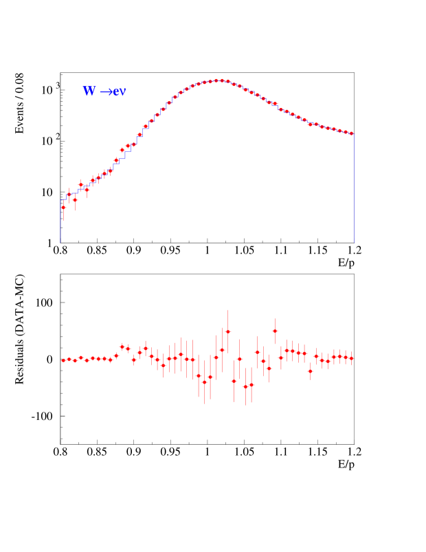
FIG. 19.: Top: $E/p$ distribution for $W$ events (points) and the best Monte Carlo fit. The solid histogram is the Monte Carlo fit normalized to data, and the points are the data. The fit reproduces the shape very well as indicated by the $\chi^{2}$/dof =0.86. Bottom: The difference between the data and the best fit simulation.

FIG. 20.: The energy resolution $\kappa$ and tracking resolution $\delta(1/p_{T})$ as determined from fits to the $E/p$ distribution in $W\rightarrow\ e\nu$ events, compared to the same resolutions determined from the $Z\rightarrow\ e^{+}e^{-}$ and $Z\rightarrow\mu^{+}\mu^{-}$ data.

The $E/p$ distribution is fit for an energy scale and tracking resolution using a binned likehood method. The method is similar to the one used to fit the $Z$ mass. The data are collected in 25 bins for the region $0.9<E/p<1.1$, containing 22,112 events as shown in Figure 19. The log likelihood is maximized with respect to $S_{E}$ and the momentum resolution simultaneously. The energy scale factor is found to be

$$S_{E}(E/p) = 0.99633\pm 0.00040{\rm(stat.)}$$ (15)

$$\pm 0.00024(\kappa)\pm 0.00035(X_{\circ})\pm 0.00018(p_{T}{\rm~{}scale}),$$

where 0.00024 comes from the uncertainty in the calorimeter resolution, 0.00035 from the uncertainty in the radiation length measurement, and 0.00018 comes from the uncertainty in the momentum scale which for this purpose is determined by the $\Upsilon$(1s) measurement (see Section III G). The result of the fit is shown in Figure 19. When we account for the nonlinearity of the calorimeter energy between $Z$ decay electrons and $W$ decay electrons as described in Section IV E, the scale factor becomes

$$S_{E}(E/p)=0.99480 \pm 0.00040{\rm~{}(stat.)}$$ (16)

$$\pm 0.00024{\rm~{}(\kappa)}\pm 0.00035{\rm~{}(X_{\circ})}\pm 0.00018{\rm~{}(p_{T}~{}scale)}$$ (17)

$$\pm 0.00075{\rm~{}(CEM~{}nonlinearity).}$$ (18)

It is in poor agreement (3.9$\sigma$ discrepant) with the energy scale determined from the $Z$ mass (Eq. 10). When this scale factor is applied to the data, the $Z$ mass is measured to be 0.52% lower than the world-average value.

The $E/p$ distribution for the $Z$ sample is also used to extract $S_{E}$. The result is:

$$S_{E}(E/p)=0.99720 \pm 0.00130{\rm~{}(stat.)}$$ (19)

$$\pm 0.00024{\rm~{}(\kappa)}\pm 0.00035{\rm~{}(X_{\circ})}\pm 0.00018{\rm~{}(p_{T}~{}scale).}$$ (20)

The systematic uncertainties with respect to $\kappa$, $X_{\circ}$, and momentum scale are common for the $W$ and $Z$ samples. The difference between this scale value and the scale from the $Z$ mass is 2.0$\sigma$. When both the $W$ and $Z$ events are combined, the discrepancy is 5.3$\sigma$.

The disagreement between the energy scale determined from the $Z$ mass (Eq. 10) with that determined by the $E/p$ distribution (Eq.s 14 and 15) is significant; therefore it would be incorrect to average the two. Moreover, the two techniques applied to the $Z$ sample use the same energy measurements, thus hinting at a systematic problem between the tracking for muons and that for electrons, or a systematic difference between the actual tracking and the tracking simulation. Another possibility is an incomplete modeling of the calorimeter response to bremsstrahlung in the tracking volume. Appendix A describes some possible causes.

As a result of this disagreement, we choose to use conservative methods for both the electron energy and muon momentum scale determination. We use the $Z\rightarrow\ e^{+}e^{-}$ mass instead of the $E/p$ distribution to set the electron energy scale since this is a direct calibration of the calorimeter measurement without reference to tracking or details of the bremsstrahlung process. Although statistically much less precise, we use the $Z\rightarrow\mu^{+}\mu^{-}$ mass instead of the $\Upsilon$(1s) or $J/\psi$ mass to set the muon momentum scale.

G Summary

The electron energy scale is determined by normalizing the measured $Z\rightarrow\ e^{+}e^{-}$ mass to the world-average mass. The measurement is limited by the finite statistics in the $Z$ peak which gives the uncertainty of 72 MeV/c² on $M_{W}$. A small nonlinearity is observed, resulting in $\Delta M_{W}=(34\pm 17)$ MeV/c². Adding these uncertainties in quadrature, the total uncertainty on $M_{W}$ due to the energy scale determination is 75 MeV/c². The energy resolution is measured from the width of the $Z\rightarrow\ e^{+}e^{-}$ peak in the same dataset: ${\sigma_{E_{T}}\over E_{T}}=\sqrt{{(13.5\%)^{2}\over{E_{T}}}+(1.53\pm 0.27)\%^{2}}.$ When the electron energy resolution is varied over this allowed range in the simulation, the measured $W$ mass changes by 25 MeV/c².

V Backgrounds

Backgrounds in the $W$ samples come from the following processes:
1. $W\rightarrow\tau\nu\rightarrow\ell\nu\nu\nu$ $W\rightarrow\tau\nu\rightarrow$ hadrons + $\nu\nu$ 2. $Z\rightarrow\ell^{+}\ell^{-}$ where the second charged lepton is not detected 3. Dijets (QCD) where jets mimic leptons 4. cosmic rays

Contributions from $Z\rightarrow\tau^{+}\tau^{-}$, $W^{+}W^{-}$, and $t\overline{t}$ are negligible. In general, backgrounds have a lower average transverse mass than $W\rightarrow\ell\nu$ decay, and, if not accounted for, will lower the fitted mass. All the background distributions as shown in Figure 21 are included in the simulation.

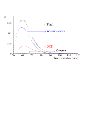
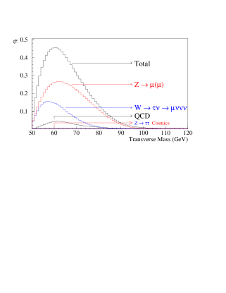
FIG. 21.: The fractions (%) of backgrounds as a function of transverse mass distribution for the $W\rightarrow\ e\nu$ sample (Top) and the $W\rightarrow\ \mu\nu$ sample (Bottom). The smallest contributor, $W\rightarrow\tau\nu\rightarrow$ hadrons + $\nu\nu$, is not shown in this figure.

A $W\rightarrow e\nu$ Backgrounds

Few $W\rightarrow\tau\nu\rightarrow e\nu\nu\nu$ events pass the kinematic cuts since the electron $E_{T}$, the total neutrino $|{\bf E_{T}}|$, and $M_{T}$ are substantially lower than those in the $W\rightarrow\ e\nu$ decay. $W\rightarrow\tau\nu\rightarrow e\nu\nu\nu$ events are estimated to be 0.8% of $W\rightarrow\ e\nu$ events in the $W$ mass fitting region. This is the largest background in the $W\rightarrow e\nu$ sample, and is also the easiest to simulate. We have also simulated the $W\rightarrow\tau\nu$ background where the $\tau$ decays hadronically. We expect it to be $(0.054\pm 0.005)$% of the $W$ sample. After $Z$ removal cuts, very few $Z\rightarrow\ e^{+}e^{-}$ events can mimic $W\rightarrow\ e\nu$ events. The Monte Carlo simulation predicts $(0.073\pm 0.011)$% of the $W$ sample in the mass fitting region to originate from $Z\rightarrow\ e^{+}e^{-}$.

Dijet events can pass the $W$ selection cuts if one of the jets mimics an electron and the other is mismeasured, creating $\not$$E_{T}$. Such events are refered to as “QCD” background. The QCD background is estimated by selecting QCD candidates from the $W$ sample without $M_{T}$ and $|{\bf u}|$ cuts and plotting distributions of $|\bf u|$ and $M_{T}$ as shown in Figure 22 (a detailed description can be found in Reference [28]). The number of QCD events predicted in the signal region “Region A” (see the top figure) is given by

$$N_{Region~{}A~{}(W)} = {N_{Region~{}A~{}(QCD)}\over N_{Region~{}B~{}(QCD)}}\times N_{Region~{}B~{}(W)}$$ (21)

$$= 249\pm 108,$$ (22)

from which we find $119\pm 56$ events or $(0.36\pm 0.17)$% of the $W$ events are in the $W$ mass fitting region. The kinematical distributions of the QCD events are derived from the $W\rightarrow\ e\nu$ sample with inverted electron quality cuts.

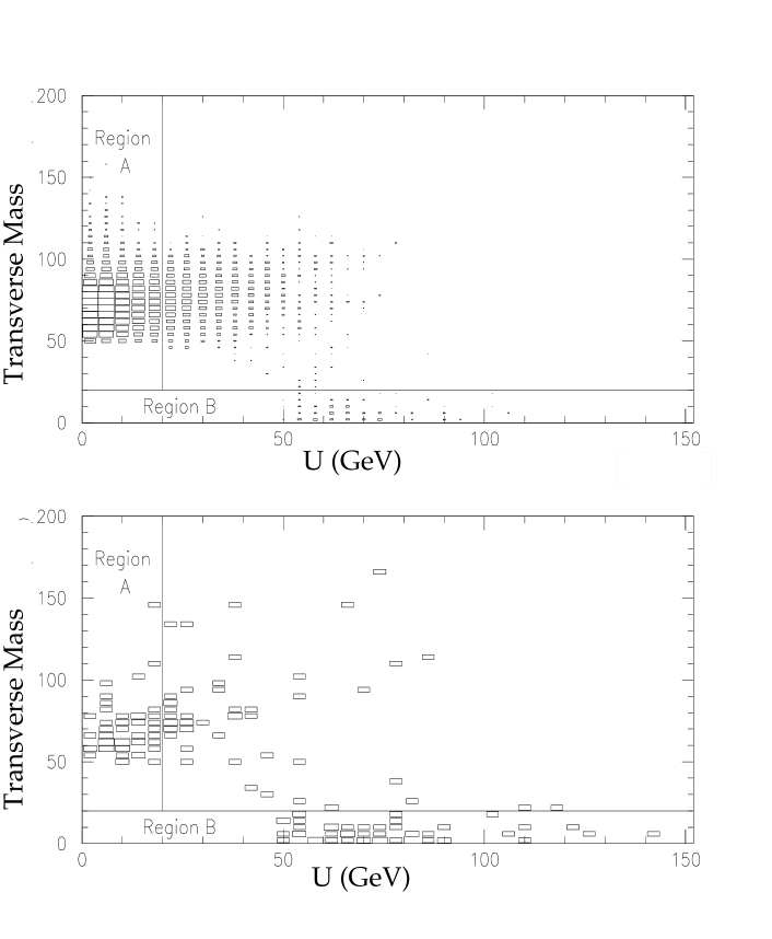
FIG. 22.: $M_{T}$ (GeV/c²) vs $|\bf u|$ distributions without $M_{T}$ and $|\bf u|$ cuts for all $W$ data (Top), and a QCD subset of the $W$ data (Bottom).

B $W\rightarrow\mu\nu$ Backgrounds

The largest background in the $W\rightarrow\mu\nu$ sample comes from the $Z\rightarrow\mu^{+}\mu^{-}$ process with one of the muons exiting at low polar angle (outside of the CTC volume) which mimics a neutrino in the calorimeters. The simulation predicts this background to be (3.6 $\pm$ 0.5)%. The uncertainty in the background estimate comes from two sources: the uncertainty in the measured tracking efficiency at large $\eta$, and the choice of parton distribution functions.

The second largest background comes from the $W\rightarrow\tau\nu$ process where $\tau\rightarrow\mu\nu\nu\nu$, which is 0.8% of the $W$ sample. The $W\rightarrow\tau\nu$ background where the $\tau$ decays hadronically is negligible. Background from QCD is estimated by using the data in a similar manner to the electron case. The $W\rightarrow\ \mu\nu$ sample is estimated to contain $(0.4\pm 0.2)$ % of its events from the QCD process. Cosmic rays can appear as two oppositely charged back-to-back tracks in $\phi$ when they cross the detector in time with ${\bar{p}}p$ collisions. Most of them are removed by the $W\rightarrow\ \mu\nu$ selection criteria such as the $Z$ removal cut or $|D_{0}|<0.2$ cm (see Section III C). The number of cosmic rays remaining in the final sample is estimated by using events which fail $|D_{0}|<$ 0.2 cm criteria, but which pass all the other selection criteria. The expected number of cosmic ray events corresponds to $(0.10\pm 0.05)$% of the $W$ sample.

C Summary

Table IX summarizes the fraction of the background events in the $W$ samples in the mass fitting region. The total backgrounds in the $W\rightarrow\ e\nu$ and $W\rightarrow\ \mu\nu$ fit region are expected to be $(1.29\pm 0.17)$% and $(4.90\pm 0.54)$%, respectively. Adding the backgrounds in the simulation leads to shifts of $(80\pm 5)$ MeV/c² and $(170\pm 25)$ MeV/c² in the $W\rightarrow\ e\nu$ and $W\rightarrow\ \mu\nu$ mass measurements, respectively.

Background source	$W\rightarrow e\nu$ sample	$W\rightarrow\mu\nu$ sample
$W\rightarrow\tau\nu\rightarrow\ell\nu\nu\nu$	0.8%	0.8%
$\mbox{$W\rightarrow\ \tau\nu$}\rightarrow$ hadrons + $\nu\nu$	$(0.054\pm 0.005)$%	$-$
Lost $Z\rightarrow\ell\ell$	$(0.073\pm 0.011)$%	$(3.6\pm 0.5)$%
QCD	$(0.36\pm 0.17)$%	$(0.4\pm 0.2)$%
Cosmic rays	$-$	$(0.10\pm 0.05)$%
Total	$(1.29\pm 0.17)$%	$(4.90\pm 0.54)$%

TABLE IX.: Backgrounds in the $W\rightarrow\ e\nu$ and $W\rightarrow\ \mu\nu$ sample in the mass fitting region.

VI $W$ Production and Decay Model

We use a Monte Carlo program to generate $W$ events according to a relativistic Breit-Wigner distribution and a leading-order ($p_{T}^{W}=0$) model of quark-antiquark annihilation. The distribution in momentum of the quarks is based on the MRS-R2 parton distribution functions (PDFs) [35]. The generated $W$ is Lorentz-boosted, in the center-of-mass frame of the quark-antiquark pair, with a transverse momentum, $p_{T}^{W}$. The $p_{T}^{W}$ spectrum is derived from the $Z\rightarrow\ e^{+}e^{-}$ and $Z\rightarrow\mu^{+}\mu^{-}$ data and a theoretical prediction for the ratio of $Z$ and $W$ $p_{T}$ spectra which is differential in the rapidity of the vector boson. The Monte Carlo program also includes QED radiative effects [31].

A Parton Distribution Functions

The uncertainty associated with PDFs is evaluated by varying the choice of PDF sets and by parametric modifications of PDFs. Figure 23 shows the CDF data on the $W$ lepton charge asymmetry [36] which is sensitive to the ratio of $d$ to $u$ quark densities $(d/u)$ at a given parton momentum fraction, $x$. Of all modern PDFs, the two giving the best agreement, MRST [37] and CTEQ-5 [38], are shown. Unfortunately the agreement even with these PDFs is barely satisfactory. Hence we follow reference [40] in making parametric modifications to the MRS family of PDFs. These modifications with retuned parameters are listed in Table X and their predictions are compared to the $W$ lepton charge asymmetry measurement and the NMC $d/u$ data [41] in Figure 24. From the variation among the six reference PDFs, an uncertainty of 15 MeV/c² is taken which is common to the electron and muon analyses.

FIG. 23.: The CDF $W$ lepton charge asymmetry measurement compared to predictions using the DYRAD calculations with MRST (solid) and CTEQ-5 (dashed) PDFs.

PDFs	Modification
MRST	$d/u\rightarrow d/u\times(1.07-0.07e^{-8x})$
MRS-R2	$d/u\rightarrow d/u+0.11x\times(1+x)$
MRS-R1	$d/u\rightarrow d/u\times(1.00-0.04e^{-\frac{1}{2}(\frac{(x-0.07)}{0.015})^{2}})$

TABLE X.: Reference PDFs and modifications.

FIG. 24.: (a) The CDF measurement of the $W$ lepton charge asymmetry compared with the six reference PDFs. The upper and lower dotted curves are MRS-R2 and MRS-R2 modified, the upper and lower dashed curves are MRS-R1 modified and MRS-R1, and the upper and lower solid curves in $|\eta|<1$ are MRS-T and MRS-T modified, respectively. (b) The NMC $d/u$ data evolved to $Q^{2}=M_{W}^{2}$. The gray bands represent the range spanned by the six reference PDFs.

B $W$ Transverse Momentum Spectrum

The spectrum of $W$ transverse momentum, $p_{T}^{W}$, is needed to simulate the lineshape of transverse mass. The $W$ mass measurement uses events at low $p_{T}^{W}$ where the theoretical calculations are not reliable. It would be difficult to extract $p_{T}^{W}$ from the $W$ data because the neutrino momentum is not well measured. However one can model $p_{T}^{W}$ through a measurement of $p_{T}^{Z}$, which can be measured accurately using the charged leptons from the $Z$ decays. Theoretical calculations predict the cross-section ratio of $W$’s and $Z$’s as a function of $p_{T}$ with small uncertainty since the production mechanisms are similar [42]. The measurement of $p_{T}^{Z}$ is combined with the theoretical calculations of the ratio to derive $p_{T}^{W}$. This procedure is applied separately to the muon and electron samples, so the derived $p_{T}^{W}$ distributions are essentially independent although compatible.

For each $Z$ sample, a functional form for the $Z$ $p_{T}$ distribution is assumed for input to a Monte Carlo generator. The lepton response is modeled according to detector resolution and acceptance. The parameters of the assumed functions are fit to give agreement with the observed $Z$ $p_{T}$ distributions. The observed $Z$ $p_{T}$ distributions are shown in Figure 25 and are compared with the simulation which uses the best fit parameters for the input $p_{T}^{Z}$ distribution.

FIG. 25.: The observed $Z$ $p_{T}$ distributions (points) for the (a) $Z\rightarrow\ e^{+}e^{-}$ and (b) $Z\rightarrow\mu^{+}\mu^{-}$ sample are compared with the Monte Carlo simulation. The solid line in (a) shows the best fit parameters for the input $p_{T}^{Z}$ distribution, whereas the shaded band in (b) shows the $1\sigma$ variation of the fit parameters.

Resummed calculations [43, 44] are used for correcting the difference between the $W$ and $Z$ $p_{T}$ distributions, in terms of the ratio of the two distributions. As shown in Figure 26 (a), (b) and (c), the ratio is between 0.9 and 1.0 over the $p_{T}$ range of interest. Effects from the large ratio at $p_{T}\sim$ 0 is very small since $d\sigma/d(p_{T})\rightarrow 0$ as $p_{T}\rightarrow 0$. The variation of the ratio is studied by varying PDFs and nonperturbative parameters in the resummed calculations, and by calculating it in two different resummed schemes, one in impact parameter space [43] and the other in $p_{T}$ space [44]. There is a rapidity ($y^{boson}$) dependence to the $p_{T}$ distribution, illustrated in Figure 26 (d) and (e). This rapidity dependence is taken into account when $p_{T}^{W}$ is derived from $p_{T}^{Z}$. As indicated in Figure 26, the range of the possible ratio and rapidity dependence variation is about 2%.

The extracted $p_{T}^{W}$ distribution for the muon channel at the generation level is shown in Figure 27 (b). The shaded band represents the total uncertainty on the $p_{T}^{W}$ distribution. The dominant uncertainty comes from the finite statistics of the $Z$ sample. The theoretical uncertainty in the $p_{T}$ ratio and rapidity dependence is small. The fractional uncertainties on the $p_{T}^{W}$ distribution from the statistics and theoretical calculations are shown in Figure 27 (a).

The uncertainty on the $W$ mass is evaluated by varying the $p_{T}^{W}$ distribution within the shaded band in Figure 27 (a). The finite statistics of the $Z$ sample contributes independent uncertainties of 15 MeV/c² and 20 MeV/c² for the $W\rightarrow\ e\nu$ and $W\rightarrow\ \mu\nu$ channel. The contribution of the theoretical uncertainty is 3 MeV/c² which is common for the electron and muon channel.

FIG. 26.: The ratios of the $p_{T}^{W}$ to $p_{T}^{Z}$ distribution from resummed calculations in impact parameter space showing (a) PDF dependence, and (b) nonperturbative parameter dependence. The ratios in impact parameter space and $p_{T}$ space are compared in (c). The ratio of $p_{T}^{Z}$ at $y^{Z}=0.3$ to $p_{T}^{Z}$ for (d) $0<y^{Z}<0.25$, and (e) $0.25<y^{Z}<0.5$.

FIG. 27.: (a) The fractional uncertainties on $p_{T}^{W}$ as a function of $p_{T}^{W}$. The solid lines show the uncertainty due to the $Z$ statistics and the shaded band the uncertainty due to the theoretical calculations. (b) The $p_{T}^{W}$ distribution extracted from the $p_{T}^{Z}$ distribution and the theoretical calculations of $p_{T}^{W}/p_{T}^{Z}$ for the $W\rightarrow\ \mu\nu$ mass measurement. The band represents the uncertainties.

C QCD Higher Order Effects

The $W$ bosons are treated as spin-one particles and decay via the weak interaction into a charged lepton ($e$, $\mu$ or $\tau$) and a neutrino. The charged leptons are produced with an angular distribution determined by the ${\cal{O}}({{\alpha}_{s}^{2}})$ calculation of [45] which, for $W^{+}$ bosons with a helicity of –1 with respect to the proton direction, has the form :

$$\frac{d\sigma}{d\cos{\theta_{\rm CS}}}\propto 1+a_{1}(p_{T})\cos{\theta_{\rm CS}}+a_{2}(p_{T})\cos^{2}{\theta_{\rm CS}}$$ (23)

where $p_{T}$ is the transverse momentum of the $W$ and $\theta_{\rm CS}$ is the polar direction of the charged lepton with respect to the proton direction in the Collins-Soper frame [46]. $a_{1}$ and $a_{2}$ are $p_{T}$ dependent parameters. For $p_{T}$ = 0, $a_{1}=2$ and $a_{2}=1$ providing the angular distribution of a $W$ boson fully polarized along the proton direction. For the $p_{T}^{W}$ values relevant to the $W$ mass analysis $(p_{T}^{W}<\sim 30)$, the change in $W$ polarization as $p_{T}^{W}$ increases only causes a modest change in the angular distribution of the decay leptons [45]. The uncertainty is negligible.

D QED Radiative Effects

$W\gamma$ production and radiative $W$ decays ($W\rightarrow\ell\nu\gamma$) are simulated using the calculation by Berends and Kleiss [31, 32]. Most photons tend to be collinear with the lepton, often showering in the same calorimeter towers as the lepton. For the electron channel, these photons are merged with the electron cluster; for the muon channel, they reduce the muon momenta by their energy. Radiative effects from collinear photons are thus expected to be larger in the muon channel. Photons not collinear with the lepton are included in the calculation of ${\bf u}$ (see Figure 2), and have an effect that is similar in both the electron and muon channels.

Shifts in the $W$ mass due to radiative effects are estimated to be $(-65\pm 20)$ MeV/c² and $(-168\pm 10)$ MeV/c² for the electron and muon channel, respectively. Uncertainties of the radiative effects are estimated from uncertainties in the theoretical calculation and in the calorimeter response to the photons. The Berends and Kleiss calculation [31] does not include all the radiative Feynman diagrams. For example, it does not include initial state radiation ($t$- and $u$-channel diagrams) and allows a maximum of one photon. The effect arising from the missing diagrams is evaluated by incorporating the PHOTOS package [33] which allows two photon emissions, and the calculation by U. Baur et al. [34] who have recently developed a complete $O(\alpha)$ Monte Carlo which incorporates the initial state QED radiation from the quark-lines and the interference between the initial and final state radiation as well as including a correct treatment of the final state soft and virtual photonic corrections. The effects on $M_{W}$ from the former case are less than 10 MeV/c² for the $W\rightarrow\ e\nu$ channel and less than 5 MeV/c² for the $W\rightarrow\ \mu\nu$ channel. The effects on $M_{W}$ from the latter case are less than 20 MeV/c² for the $W\rightarrow\ e\nu$ channel and $\sim$10 MeV/c² for the $W\rightarrow\ \mu\nu$ channel. The uncertainty in the calorimeter response to the photons well-separated from the $W$ decay lepton, is evaluated by varying the photon energy threshold, the photon fiducial region, and the photon energy resolution. The effect is 3 MeV/c² on the $W$ mass.

E Summary

The uncertainty associated with PDFs is evaluated by varying the choice of PDF sets. It is estimated to be 15 MeV/c² which is common to the electron and muon analyses. The $p_{T}^{W}$ spectrum is derived from the $Z\rightarrow\ e^{+}e^{-}$ and $Z\rightarrow\mu^{+}\mu^{-}$ data and a theoretical prediction for the ratio of $Z$ and $W$ $p_{T}$ spectra differential in the rapidity of the vector boson. The corresponding uncertainty in the $W$ mass is dominated by $Z$ statistics. It is 15 MeV/c² for the $W\rightarrow\ e\nu$ channel and 20 MeV/c² for the $W\rightarrow\ \mu\nu$ channel. A common uncertainty of 3 MeV/c² comes from the theoretical prediction for the ratio. The uncertainty in the $W$ mass due to QED radiative effects is estimated to be 20 MeV/c² to the $W\rightarrow\ e\nu$ channel, and 10 MeV/c² to the $W\rightarrow\ \mu\nu$ channel.

VII Recoil Measurement and Model

The transverse mass distribution used for the $W$ mass measurement is reconstructed using the $\bf E_{T}$ of the charged leptons (described in Section III and IV) and the neutrinos. The transverse energy of the neutrino is inferred from the charged lepton $\bf E_{T}$ and the recoil energy $\bf u$ (see Figure 2). This section describes the reconstruction of $\bf u$, and an empirical model of the detector response to $\bf u$ which is implemented in the simulation. Since the $W$ and $Z$ share a common production mechanism and are close in mass, the recoil model is based mainly on $Z\rightarrow\ell^{+}\ell^{-}$ decays.

A Recoil Reconstruction

The recoil vector $\bf u$ is calculated by summing over electromagnetic and hadronic calorimeter towers within the detector range $|\eta|<3.6$,

$${\bf u}=(u_{x},u_{y})=\Sigma_{\rm towers}E\sin\theta(\cos\phi,\sin\phi).$$ (24)

Table XI lists tower thresholds for online (Level-3) reconstruction and this analysis. The thresholds for this analysis correspond to 5 times the calorimeter noise level.

Calorimeter	Online threshold (GeV)	Analysis threshold (GeV)
Central EM	0.1	0.1
Central Had.	0.1	0.185
Plug EM	0.3	0.15
Plug Had.	0.5	0.445
Forward EM	0.5	0.2
Forward Had.	0.8	0.73

TABLE XI.: Tower energy thresholds used to reconstruct $\bf u$ both in online and in this analysis.

There are two contributions to the recoil vector $\bf u$. The first contribution is the energy of the initial state gluons radiated from the quarks that produce the $W$ or $Z$ boson. This energy balances the $p_{T}$ of the boson. The second is the energy associated with multiple interactions and the remnants of the protons and antiprotons that are involved in the $W$ or $Z$ production. The latter energy is referred to as the underlying energy. It is manifested in $\Sigma E_{T}$, where

$$\Sigma E_{T}=\Sigma_{\rm towers}E\sin\theta=\Sigma_{\rm towers}E_{T}.$$ (25)

The lepton energy should not be included in the $\bf u$ calculation, and thus the towers containing energy deposited by the lepton are excluded in the sum. This procedure removes two towers for muons, and two or three towers for electrons. If the center of the electron shower is more than 10 cm away from the azimuthal center of the tower ($|x|>10$ cm), there will be leakage in the azimuthally adjacent towers which are also removed. This procedure removes not only the lepton energy, but also the underlying energy which needs to be added back to the sum. The underlying energy is estimated from the energy in calorimeter towers away from the lepton in the $W$ data. In the muon analysis, this energy is added back to the $\bf u$ calculation. In the electron analysis, rather than correcting $\bf u$, the same amount of energy is removed from the Monte Carlo simulation.

B Recoil Model

For the purposes of modeling the response and resolution, it is natural to define $\bf u$ in terms of the components $u_{1}$ and $u_{2}$, anti-parallel and perpendicular to the boson direction, respectively. The average value of $u_{1}$ is the average calorimeter response balancing the boson $p_{T}$, and the average value of $u_{2}$ is expected to be zero. $u_{1}$ and $u_{2}$ are parameterized in the form

$$\left(\begin{array}[]{c}u_{1}\\ u_{2}\end{array}\right)=\left(\begin{array}[]{c}f(p_{T}^{boson})\\ 0\end{array}\right)+\left(\begin{array}[]{c}G_{1}(\sigma_{1})\\ G_{2}(\sigma_{2})\end{array}\right)$$ (26)

where $G_{1}(\sigma_{1})$ and $G_{2}(\sigma_{2})$ are Gaussian distributed random variables of mean zero and widths $\sigma_{1}$ and $\sigma_{2}$, and the quadratic function $f(p_{T}^{boson})$ is the response function to the recoil energy. A detailed description can be found in Reference [28].

The resolutions $\sigma_{1}$ and $\sigma_{2}$ are expected to be dependent on $\Sigma E_{T}$. For the minimum bias events which represent the underlying event in the $W$ and $Z$ sample, the resolutions $\langle\sigma_{x}\rangle$ and $\langle\sigma_{y}\rangle$ are well parameterized with $\Sigma E_{T}$. A fit to the data, as shown in Figure 28, gives

$$\sigma_{mbs}(\mbox{$\Sigma E_{T}$})=0.324\times(\mbox{$\Sigma E_{T}$})^{0.577}$$ (27)

where $\sigma_{mbs}(\mbox{$\Sigma E_{T}$})$ and $\Sigma E_{T}$ are calculated in GeV. For the $W$ and $Z$ events, a good description of the resolution requires additional parameters which accont for its boson $p_{T}$ dependence; the initial state gluons balancing the boson $p_{T}$ produce jets which contribute to the resolution differently than the underlying energy. In order to allow this resolution difference, the widths are parameterized in the form

$$\left(\begin{array}[]{c}\sigma_{1}\\ \sigma_{2}\end{array}\right)=\sigma_{mbs}(\mbox{$\Sigma E_{T}$})\times\left(\begin{array}[]{c}1+s_{1}\cdot(p_{T}^{boson})^{2}\\ 1+s_{2}\cdot(p_{T}^{boson})^{2}\end{array}\right)$$ (28)

for the electron channel and

$$\left(\begin{array}[]{c}\sigma_{1}\\ \sigma_{2}\end{array}\right)=\sigma_{mbs}(\mbox{$\Sigma E_{T}$})\times\left(\begin{array}[]{c}\alpha_{1}+\beta_{1}\cdot p_{T}^{boson}\\ \alpha_{2}+\beta_{2}\cdot p_{T}^{boson}\end{array}\right)$$ (29)

for the muon channel, where $s_{1}$, $s_{2}$, $\alpha_{1}$, $\alpha_{2}$, $\beta_{1}$, and $\beta_{2}$ are free parameters. Although the two channels use different formulae, the fitted funtions are consistent with each other – $\alpha_{1}$ and $\alpha_{2}$ are close to 1 and the difference between the linear term and the quadratic term is within the statistical uncertainty of the $Z$ sample. The argument $\Sigma E_{T}$ in Eq.s 28 and 29 comes from the $\Sigma E_{T}$ distributions of the $W$ and $Z$ data. The $\Sigma E_{T}$ distributions in various $p_{T}^{Z}$ bins are shown in Figure 29. They are nicely fit to $\Gamma$-distributions

$$\gamma(\mbox{$\Sigma E_{T}$};a,b)={a^{b}(\mbox{$\Sigma E_{T}$})^{b-1}e^{-a(\mbox{$\Sigma E_{T}$})}\over\Gamma(b)}$$ (30)

where $a$ and $b$ are fit parameters, and $b$ is a linear function of $p_{T}^{boson}$. The term $a/\Gamma(b)$ normalizes the distribution. Figure 30 shows the $\Sigma E_{T}$ distributions and fits for the $Z$ and $W$ events.

FIG. 28.: The fit for the rms of the $u_{x}$ and $u_{y}$ distributions as a function of $\Sigma E_{T}$ using the minimum bias sample.

FIG. 29.: The $\Sigma E_{T}$ distributions in 5 different $p_{T}^{Z}$ bins for the $Z\rightarrow\mu^{+}\mu^{-}$ data are shown: (a) for $p_{T}^{Z}<5$ GeV, (b) for $5<p_{T}^{Z}<10$ GeV, (c) for $10<p_{T}^{Z}<20$ GeV, (d) for $20<p_{T}^{Z}<30$ GeV, and (e) for $30<p_{T}^{Z}<50$ GeV.

FIG. 30.: The $\Sigma E_{T}$ distributions for (a) the $W\rightarrow\ e\nu$ sample, (b) the $Z\rightarrow\ e^{+}e^{-}$ sample, (c) the $W\rightarrow\ \mu\nu$ sample, and (d) the $Z\rightarrow\mu^{+}\mu^{-}$ sample. The solid lines are fits to the functions described in Eq. 30.

FIG. 31.: The $\langle u_{1}\rangle$ versus $p_{T}^{Z}$ (solid lines) as derived from $Z$ sample fits for (a) the electron channel and (b) the muon channel. The fits are compared with the data points.

FIG. 32.: The fit of the $u_{1}$ and $u_{2}$ distributions in ranges of $Z$ $p_{T}$ in the muon sample, illustrating the adequacy of assuming Gaussian resolution(solid lines).

The $Z$ data provide $u_{1}$, $u_{2}$, $\Sigma E_{T}$, and the $p_{T}$ of the $Z$. The parameters in Eqs. 26, 30, 28, and 29 are derived by fitting to these variables. Figure 31 compares $\langle u_{1}\rangle$ as a function of $p_{T}^{Z}$ from the $Z$ data with the fit functions $f(p_{T}^{Z})$ described in Eq. 26. The validity of a Gaussian parameterization in Eq. 26 is illustrated in Figure 32. The parameterization of the recoil response model is further cross-checked by distributions of $u_{1}$, $u_{2}$, and $|\bf u|$. As shown in Figure 33, they all agree well. The $u$ resolutions in the $Z\rightarrow\mu^{+}\mu^{-}$ data are shown as a function of $p_{T}^{Z}$ in Figure 34, where the data is compared with the recoil model with (the solid histograms) and without (the dashed histograms) including the effect of gluons against the $W$. As expected, the resolution gets worse in $u_{1}$ as the jet structure of the recoil becomes apparent, increasing $\Sigma E_{T}$ in the $u_{1}$ direction.

While the $Z$ sample, where the boson $p_{T}$ is well understood, allows the unfolding of response and resolution, the $W$ samples do not allow these effects to be separately understood. However, the $W$ samples can be used to optimize the model parameters for the $W$ data while preserving a good description of the $Z$ data. This is demonstrated in Figure 35. The ultimate recoil model includes the $\bf|u|$ and $\rm{u_{\perp}}$ (the component of $\bf u$ perpendicular to the lepton direction) distributions from the $W$ data in the fit.

FIG. 33.: (a) $u_{1}$, (b) $u_{2}$, and (c) $|\bf u|$ distributions for the $Z\rightarrow\mu^{+}\mu^{-}$ data. The histograms are the simulation using the recoil model parameters.

FIG. 34.: $\sigma(u_{1})$ and $\sigma(u_{2})$ as a function of $p_{T}^{Z}$ for the $Z\rightarrow\mu^{+}\mu^{-}$ sample. The points are the data, and the solid histograms are the simulation using the recoil model parameters. The dashed histograms show $\sigma_{mbs}(\Sigma E_{T})$, the resolutions of the underlying energy.

FIG. 35.: The muon $Z$ fits separately constrain resolution and response, as shown by the ellipse, while the $W$ data gives a further correlated constraint, as shown by the band. This is obtained from the Monte Carlo studies.

C Comparison of Data and Simulation in the $W$ Samples

This section compares the data with the simulation which uses the best fit parameters of the modeling. The $W$ data is more naturally described in terms of components $\rm{u_{\parallel}}$ and $\rm{u_{\perp}}$ of recoil defined with respect to the charged lepton direction – the component along the lepton direction and the component perpendicular to the lepton direction, respectively (see Figure 36). The $|\bf u|$ and $\rm{u_{\parallel}}$ distributions and residuals are shown in Figure 37 and Figure 38. The $\rm{u_{\perp}}$ distribution is shown in Figure 39. The means for $\rm{u_{\perp}}$ are consistent with zero and the other $\bf u$ projection numbers are listed in Table XII. The models reproduce the basic characteristics well.

FIG. 36.: Kinematics of leptons from the $W$ decay and the transverse energy vector recoiling against the $W$, as viewed in the plane transverse to the antiproton-proton beams. $\rm{u_{\parallel}}$ is the component of ${\bf u}$ along the lepton direction and $\rm{u_{\perp}}$ the component of ${\bf u}$ perpendicular to the lepton direction.

FIG. 37.: The (a) $|\bf u|$ and (c) $\rm{u_{\parallel}}$ distribution distribution for the $W\rightarrow\ e\nu$ sample. The points (histograms) are the data (simulation). The differences between the data and the simulation are shown in (b) and (d).

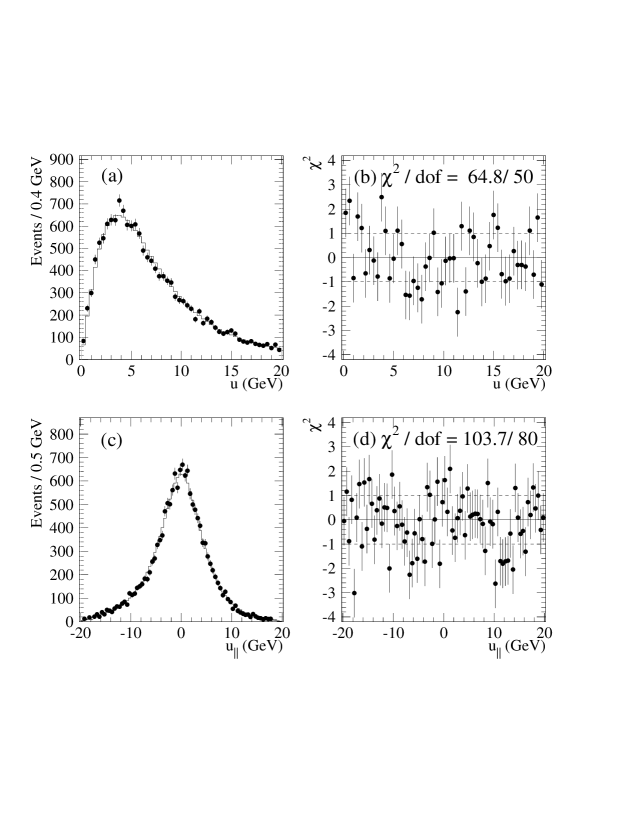
FIG. 38.: The (a) $|\bf u|$ and (c) $\rm{u_{\parallel}}$ distribution for the $W\rightarrow\ \mu\nu$ sample. The points (histograms) are the data (simulation). The differences between the data and the simulation normalized by the statistical uncertainty are shown in (b) and (d).

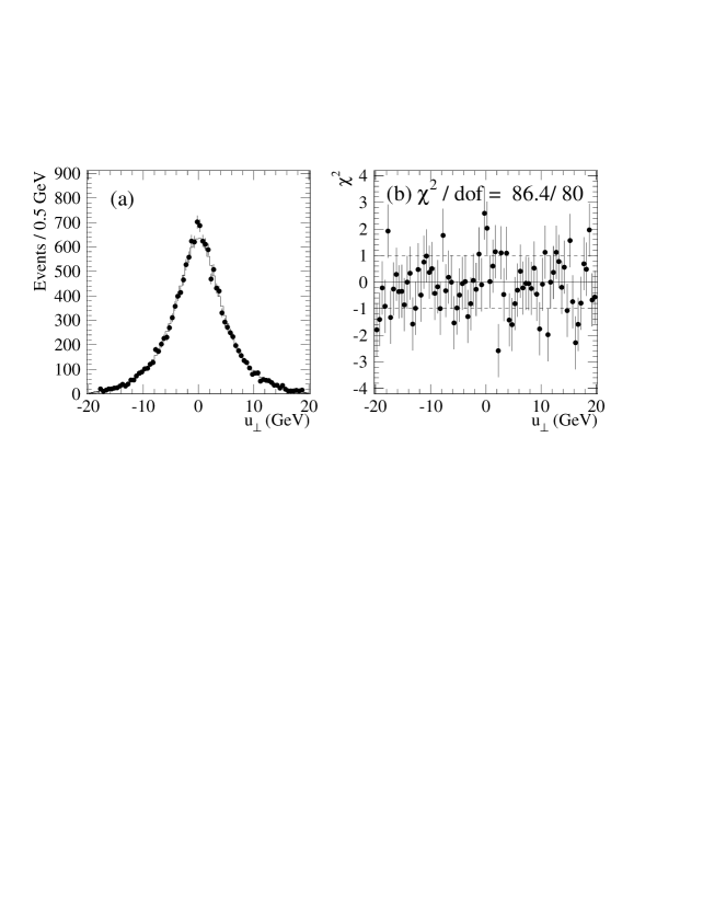
FIG. 39.: (a) The $\rm{u_{\perp}}$ distribution for the $W\rightarrow\ \mu\nu$ sample. The points (histogram) are the data (simulation). (b) The difference between the data and the simulation normalized by the statistical uncertainty.

Quantity	Mode	Data	Simulation
$\sigma^{\rm rms}(\mbox{$\rm{u_{\perp}}$})$	e$\nu$	$5.684\pm 0.034$ GeV	$5.765$ GeV
$\sigma^{\rm rms}(\mbox{$\rm{u_{\perp}}$})$	$\mu\nu$	$5.640\pm 0.065$ GeV	$5.672$ GeV
$\sigma^{\rm rms}(\mbox{$\rm{u_{\parallel}}$})$	e$\nu$	$5.877\pm 0.024$ GeV	$5.827$ GeV
$\sigma^{\rm rms}(\mbox{$\rm{u_{\parallel}}$})$	$\mu\nu$	$5.732\pm 0.069$ GeV	$5.750$ GeV
$\langle\mbox{$\rm{u_{\parallel}}$}\rangle$	e$\nu$	$-0.573\pm 0.034$ GeV	$-0.639$ GeV
$\langle\mbox{$\rm{u_{\parallel}}$}\rangle$	$\mu\nu$	$-0.436\pm 0.048$ GeV	$-0.422$ GeV

TABLE XII.: Widths and means for recoil response projections for data and simulation. The simulation includes the $W$ constraint and background bias. Uncertainties shown here are only statistical, and do not include systematic uncertainties due to $p_{T}^{W}$ and the recoil model.

One can further examine whether or not the model describes correlations among variables. The distributions in $\rm{u_{\parallel}}$ are examined in four bins of $|{\bf u}|$, shown for the electron analysis in Figure 40 and for the muon analysis in Figure 41. The correlation of $\rm{u_{\parallel}}$ and transverse mass is illustrated in Figure 42 and the trend of $\langle\mbox{$\rm{u_{\parallel}}$}\rangle$ with azimuthal angle between the lepton and $\bf u$ is shown in Figure 43. As indicated in these figures, the simulation well represents the data.

FIG. 40.: The $\rm{u_{\parallel}}$ distributions for the $W\rightarrow\ e\nu$ sample in four bins of $|{\bf u}|$. The points are the data, and the histograms the simulation.

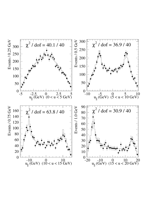
FIG. 41.: The $\rm{u_{\parallel}}$ distributions for the $W\rightarrow\ \mu\nu$ sample in four bins of $|{\bf u}|$. The points are the data, and the histograms the simulation.

FIG. 42.: (a) The average value of ${\rm u_{\parallel}}$ as a function of $M_{T}$ for the $W\rightarrow\ e\nu$ sample. The points are the data, and the solid histogram is for the simulation. (b) Residuals between the data and the simulation.

FIG. 43.: $\langle\mbox{$\rm{u_{\parallel}}$}\rangle$ as a function of azimuthal angle between the lepton and $\bf u$ for the $W\rightarrow\ \mu\nu$ sample. The points are the data and the histogram is the simulation.

D Uncertanties on $M_{W}$

The uncertainty on the $W$ mass is evaluated by varying the model parameters within their uncertainties. The size of the parameter uncertainties is taken from the $Z$ statistics and does not include the reduction produced by including the $W$ data in the model. For each set of model parameters a set of transverse mass templates are produced which are fit to the transverse mass distributions of the data and a standard Monte Carlo template. The rms of $M_{W}$ values obtained from the fit to the Monte Carlo template is 37 MeV/c² for the electron channel and 35 MeV/c² for the muon channel.

E Summary

The detector response to the recoil energy against the $W$ is modeled primarily using the $Z\rightarrow\ell^{+}\ell^{-}$ data. The $W$ data are used to optimize the model. The model is empirical in the sense that its form is justified by the data and its parameters determined from the data. The modeling procedure is applied separately to the muon and electron samples, so the uncertainties on the $W$ mass due to the recoil model are essentially independent. The parametrizations are compatible in the two channels.

The uncertainty on the $W$ mass is evaluated by producing a set of transverse mass templates with the model parameters allowed within their uncertainties, and fitting to the transverse mass distributions of the data and a standard Monte Carlo template. It is 37 MeV/c² for the electron channel and 35 MeV/c² for the muon channel.

VIII Results and Conclusions

This section summarizes the $W$ mass results. Cross-checks which support the results are discussed. The results of the two lepton channels are combined with previous CDF measurements. The combined result is compared with other measurements and with global fits to all precise electroweak measurements which predict a $W$ mass as a function of the Higgs boson mass.

A Fitting Procedure

The $W$ mass is obtained from a binned maximum likelihood fit to the transverse mass spectrum. This spectrum cannot be predicted analytically and must be simulated using a Monte Carlo program which produces the shape of the transverse mass distribution as a function of $M_{W}$. This program incorporates all the experimental effects relevant to the analysis, including $W$ production and decay mechanisms as described in Section VI, the detector acceptance for the charged leptons from the $W$ decay, the detector responses and resolutions of the leptons as described in Sections III and IV, and the detector response and resolution of the recoil energy against the $W$ as described in Section VII. The Monte Carlo program generates $M_{T}$ distributions used as templates for discrete values of $M_{W}$. The width of the $W$, $\Gamma_{W}$, is taken as the Standard Model value [47] for that $W$ mass. The transverse mass distribution templates also include the background contributions. The mass fit compares the data transverse mass distribution to the templates.

The transverse mass fitting procedure is tested by using large Monte Carlo samples and by generating pseudo-samples of the size of the data and extracting a mass value for each dataset. We investigated the bias in the fit and confirmed the statistical errors returned by the fits. The results are illustrated for the muon fit in Figure 44. No biases are observed in the fitting procedure and the fit errors returned by the simulation datasets and the variation in returned mass values are consistent with the statistical uncertainties of the fits to the data.

FIG. 44.: (a) Difference between the input $M_{W}$ values and the returned values by fits to Monte Carlo pseudo-samples. Each sample is 100 times the size of the $W\rightarrow\ \mu\nu$ data. (b) The (statistical) error returned by fitting 1000 Monte Carlo pseudo datasets of the same size as the $W\rightarrow\ \mu\nu$ data.

B The $W$ Mass Measurement

The fit results yield the measurements of the $W$ mass in the electron and muon channels. They are:

$$M_{W}^{e}=80.473\pm 0.065~{}{\rm(stat.)}\pm 0.092~{}{\rm(syst.)}~{}{\rm GeV/c^{2}}$$

and

$$M_{W}^{\mu}=80.465\pm 0.100~{}{\rm(stat.)}\pm 0.103~{}{\rm(syst.)}~{}{\rm GeV/c^{2}}.$$

The negative log likelihood distribution for the muon sample is shown in Figure 45 as a function of $M_{W}$. A similar distribution is obtained for the electron sample. The transverse mass distributions for the $W\rightarrow\ e\nu$ and $W\rightarrow\ \mu\nu$ samples are compared to the simulation with the best fits in Figures 46 and 47. The fit curves give $\chi^{2}$/dof of 32.4/35 and 60.6/70 for the electron and muon samples, respectively. If we extend the region of comparison from $65<M_{T}<100$ GeV/c² to $50<M_{T}<120$ GeV/c², the curves give $\chi^{2}$/dof of 82.6/70 and 147/131, and Kolmogornov-Smirnov (KS) probabilities of 16% and 21%.

FIG. 45.: The deviation of the negative log likelihood from the minimum for the $W\rightarrow\ \mu\nu$ sample. The $W$ width is fixed at the Standard Model value in the fit.

FIG. 46.: $W$ Transverse mass distributions compared to the best fit for the $W\rightarrow\ e\nu$ channel.

FIG. 47.: $W$ Transverse mass distributions compared to the best fit for the $W\rightarrow\ \mu\nu$ channel.

A summary of all systematic uncertainties is given in Table 8.1. They are estimated by measuring the subsequent shifts in $M_{W}$ when each source is varied by its uncertainty in the Monte Carlo simulation. The largest uncertainties come from the finite statistics of the $Z$ samples. The $Z$ statistics are the predominant source of the uncertainties on lepton scale, lepton resolution, the $p_{T}^{W}$ model, as well as the recoil model. As muon and electron analyses use the muon and electron $Z$ sample separately, the statistical effects are independent. The theoretical uncertainty in the $p_{T}^{W}$ distribution gives a small common-contribution. The uncertainty due to the choice of PDFs is evaluated for the muon acceptance and is essentailly the same for the electron acceptance. We take the PDF uncertainties to be identical and common for the two channels. Although the QED corrections are rather different for electrons and muons, there is common as well as independent uncertainty.

The total common uncertainty for the two lepton channels is 16 MeV/c², due almost entirely to the common determination of the parton distribution function contribution. Accounting for the correlations, the combined value is:

$$M_{W}=80.470\pm 0.089~{}{\rm GeV/c^{2}}.$$

Source of uncertainty	$W\rightarrow\ e\nu$	$W\rightarrow\ \mu\nu$	common
Lepton scale	75	85
Lepton resolution	25	20
PDFs	15	15	15
$P_{T}^{W}$	15	20	3
Recoil	37	35
Higher order QED	20	10	5
Trigger & Lepton ID bias	$-$	15$\oplus$10
Backgrounds	5	25
Total	92	103	16

TABLE XIII.: Systematic uncertainties in the $W$ mass measurement in MeV/c².

FIG. 48.: The 1-$\sigma$ and 2-$\sigma$ contours in $\Gamma_{W}$ versus $M_{W}$ of the transverse mass fit when the width is floated for (a) the $W\rightarrow\ e\nu$ channel and (b) the $W\rightarrow\ \mu\nu$ channel. The dashed lines are the predicted $\Gamma_{W}$ as a function of $M_{W}$.

C Cross-Checks of the $W$ Mass Measurement

The reliability of the measurement can be checked by fitting lepton $p_{T}$ instead of transverse mass, by subdividing the $W$ samples, and by removing the constraint on the $W$ width as a function of mass.

The $W$ width, $\Gamma_{W}$, can be extracted from the transverse mass distributions by fitting either in the region near the Jacobean edge or in the high-$M_{T}$ region. The CDF experiment measured $\Gamma_{W}$ to be $2.04\pm 0.14$ GeV using $100<M_{T}<200$ GeV/c² [48]. By generating $M_{T}$ templates at discrete values of $M_{W}$ and $\Gamma_{W}$, and allowing them to vary in the fit, one can measure both $M_{W}$ and $\Gamma_{W}$ simultaneously from the region near the Jacobean edge. Since $\Gamma_{W}$ provides similar effects to the input $p_{T}^{W}$ and the detector resolution of $\bf u$ in this region, the measurement of $\Gamma_{W}$ provides a check on the recoil and $p_{T}^{W}$ models. Figure 48 shows the 1-$\sigma$ and 2-$\sigma$ contours of the fitted $W$ width versus $W$ mass. The widths are consistent with the Standard Model: it is almost identical to the SM value for the muon channel, and about 1.5 $\sigma$ away for the electron channel. The fitted $W$ mass differs by 60 MeV/c² for the electron channel and 10 MeV/c² for the muon channel from the values with $\Gamma_{W}$ fixed. We do not derive measurements of the width from these fits due to the large systematics variations which come from changing resolutions and modeling.

The transverse momentum spectra of the leptons as shown in Figures 49 and 50 also contain $W$ mass information. $W$ mass values obtained from maximum likelihood fits are consistent with the values from the transverse mass fit. The distributions from the simulation with the best fits are compared with the data in the figures.

The $W$ mass results are cross-checked by making various selection criteria on the data and Monte Carlo simulation, and refitting for the $W$ mass. The events are divided into positively and negatively charged lepton samples. For the electon sample the charge difference listed in Table XIV involves statistical uncertainty only and corrreponds to the mass difference of $123\pm 130$ MeV/c² between the $W^{+}$ and the $W^{-}$. For the muon sample the table entries include the tracking alignment uncertainty of $50$ MeV/c². The mass difference of $136\pm 205$ MeV/c² is observed between the $W^{+}$ and the $W^{-}$. The electron and muon results are combined to give a mass difference of $127\pm 110$ MeV/c².

The samples are also partitioned into four bins of $|{\bf u}|$ as shown in Figures 51 and 52. The Monte Carlo simulation reproduces the data very well in all the $|{\bf u}|$ bins, indicating that the $W$ $p_{T}$ and recoil energy are well modeled in the simulation. When the events are partitioned into $p_{T}^{\mu}>35$ GeV/c and $p_{T}^{\mu}<35$ GeV/c samples, the $M_{T}$ shapes between the two samples (see Figure 53) are dramatically different. Yet there is good agreement between the data and simulation.

The extracted $W$ masses described above are summarized in Table XIV.

FIG. 49.: $E_{T}$ distributions of (a) electrons and (c) neutrinos in the $W\rightarrow\ e\nu$ channel. The points are the data and the histograms the best fit simulation. The differences between the data and simulation are shown in (b) and (d).

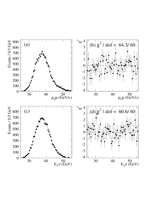
FIG. 50.: (a) $p_{T}$ distribution of muons and (c) $E_{T}$ distribution of neutrinos in the $W\rightarrow\ \mu\nu$ channel. The points are the data and the histograms the best fit simulation. (b) and (d) The difference between the data and simulation normalized by the statistical uncertainty.

FIG. 51.: Transverse mass distributions in bins of $|{\bf u}|$ for the $W\rightarrow\ e\nu$ data (triangles) and the best fit simulation (histograms). The four $|{\bf u}|$ bins are, $0<|{\bf u}|<5$ GeV (Top Left), $5<|{\bf u}|<10$ GeV (Top Right), $10<|{\bf u}|<15$ GeV (Bottom Left), and $15<|{\bf u}|<20$ GeV (Bottom Right)

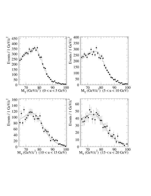
FIG. 52.: Transverse mass distributions in bins of $|{\bf u}|$ for the $W\rightarrow\ \mu\nu$ data (points) and the best fit simulation (histograms). The four $|{\bf u}|$ bins are, $0<|{\bf u}|<5$ GeV (Top Left), $5<|{\bf u}|<10$ GeV (Top Right), $10<|{\bf u}|<15$ GeV (Bottom Left), and $15<|{\bf u}|<20$ GeV (Bottom Right)

FIG. 53.: Transverse mass distributions for (a) low $p_{T}$ and (b) high $p_{T}$ muons in the $W\rightarrow\ \mu\nu$ data (squares) and simulation (lines).

Fitting	Selection	$\Delta M_{W}$ (MeV/c2) (e$\nu$)	$\Delta M_{W}$ (MeV/c2) ($\mu\nu$)
$E_{T}^{e}$, $p_{T}^{\mu}$	–	$-80\pm 60$	$-19\pm 132$
$E_{T}^{\nu}$	–	$+76\pm 60$	$-20\pm 127$
$M_{T}$	$\ell^{+}$	$+62\pm 90$	$+67\pm 145$
$M_{T}$	$\ell^{-}$	$-61\pm 90$	$-69\pm 145$
$M_{T}$	$0<|{\bf u}|<5$ GeV	$-1\pm 86$	$-41\pm 135$
$M_{T}$	$5<|{\bf u}|<10$ GeV	$-36\pm 110$	$-164\pm 169$
$M_{T}$	$10<|{\bf u}|<15$ GeV	$+161\pm 204$	$+484\pm 301$
$M_{T}$	$15<|{\bf u}|<20$ GeV	$-348\pm 385$	$+534\pm 450$

TABLE XIV.: Difference from the nominal value of extracted $M_{W}$ values from lepton transverse momentum fits and from various subsample transverse mass fits.

D Combined $W$ Mass

The issue of combining the present results with previous CDF measurements [4] merits some additional discussion since the lepton energy and momentum scales were determined differently. In particular, in our the previous analyses the electron scale was determined with the $E/p$ method. In the present work that procedure is shown to result in a $Z$ mass discrepant by $(0.52\pm 0.13)$%; in the Run IA analysis, the discrepancy was $(0.28\pm 0.24)$%. The statistics of Run IA are insufficient to distinguish the two cases – that the $E/p$ method worked well or was systematically off as indicated in the Run IB result. Moreover, the experimental conditions differ for the two runs. For example, the aging and rate effects in the CTC due to higher luminosity are more pronounced for the present work. For these reasons and because the underlying cause for the $E/p$ discrepancy remains unresolved, we believe that applying a correction factor to the Run IA result is not warranted. We prefer to average the results as published with the stated errors. Thus the combined CDF result is:

$$M_{W}=80.433\pm 0.079~{}{\rm GeV/c^{2}}.$$

This value is precise to 0.1% and corresponds to a total integrated luminosity of $\sim$105 pb^-1.

E Comparison with Other Results

The present results are compared with other published results in Table XV [3, 5, 7, 9]. The agreement is excellent. The direct measurement of the $W$ mass is an important test of the Standard Model. The $W$ mass is indirectly predicted precisely by including loop corrections involving the top quark and Higgs boson. The corresponding implication for the Higgs boson mass is shown in Figure 54. Our result agrees well with the Standard Model, and when combined with all other electroweak results [9] prefers a light Higgs boson.

UA2	$80.360\pm 0.370$ GeV/c2
CDF	$80.433\pm 0.079$ GeV/c2
D0	$80.474\pm 0.093$ GeV/c2
ALEPH	$80.418\pm 0.076$ GeV/c2 upto $\sqrt{s}$ = 189 GeV
	$80.423\pm 0.123$ GeV/c2 upto $\sqrt{s}$ = 183 GeV
DELPHI	$80.270\pm 0.144$ GeV/c2 upto $\sqrt{s}$ = 183 GeV
L3	$80.610\pm 0.150$ GeV/c2 upto $\sqrt{s}$ = 183 GeV
OPAL	$80.432\pm 0.080$ GeV/c2 upto $\sqrt{s}$ = 189 GeV (preliminary)
	$80.380\pm 0.130$ GeV/c2 upto $\sqrt{s}$ = 183 GeV
Indirect Meas.	$80.381\pm 0.026$ GeV/c2

TABLE XV.: Measurements of the $W$ mass. CDF and D0 measurements have a common error mostly due to Parton Distribution Functions. The LEP II measurements have common errors including the LEP beam energy. The indirect measurement includes the LEP and SLC $Z$ pole measurements, the $\nu$N measurement, and the Tevatron Top mass measurements.

F Conclusions

We have measured the $W$ mass to be $M_{W}=80.470\pm 0.089~{}{\rm GeV/c^{2}}$ using data with an integrated luminosity of $\sim$85 pb^-1 collected from 1994 to 1995. When combined with previously published CDF data, we obtain $M_{W}=80.433\pm 0.079~{}{\rm GeV/c^{2}}$.

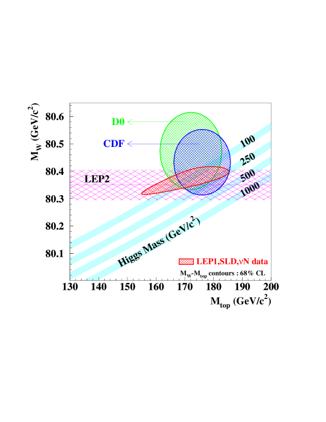
FIG. 54.: The direct measurements of the $W$ and top quark mass from CDF and DO/ experiments, the direct measurement of the $W$ mass from LEP II experiments, and the indirect $W$ and top mass measurement from LEP, SLC, and Tevatron neutrino experiments. The curves are from a calculation of the dependence of the $W$ mass on the top mass in the Standard Model using several Higgs boson masses. The band on each curve is the uncertainty obtained by folding in quadrature uncertainties on $\alpha(M_{Z}^{2})$, $M_{Z}$, and $\alpha_{s}(M_{Z}^{2})$. The uncertainty is dominated by the hadronic contribution to $\alpha(M_{Z}^{2})$, $\Delta\alpha_{had}=0.028\pm 0.0007$ (Ref.48).

Acknowledgments

We thank the Fermilab staff and the technical staffs of the participating institutions for their vital contributions. This work was supported by the U.S. Department of Energy and National Science Foundation; the Italian Istituto Nazionale di Fisica Nucleare; the Ministry of Education, Science, Sports and Culture of Japan; the Natural Sciences and Engineering Research Council of Canada; the National Science Council of the Republic of China; the Swiss National Science Foundation; the A. P. Sloan Foundation; the Bundesministerium fuer Bildung und Forschung, Germany; and the Korea Science and Engineering Foundation. We also thank Ulrich Baur and Keith Ellis in support and advice.

A Discussion of Discrepancy between $M_{Z}$ and $E/p$ Methods

The calorimeter energy scale for the $W$ mass measurement in this paper is set using the invariant mass distribution of $Z\rightarrow\ e^{+}e^{-}$ events. Ideally, the $E/p$ distribution would be used to set the energy scale where the momentum scale is determined by the $\Upsilon\rightarrow\mbox{$\mu^{+}\mu^{-}$}$ data. The $E/p$ distribution has a smaller statistical uncertainty than the method of using the $Z\rightarrow\ e^{+}e^{-}$ mass because it makes use of the higher statistics of the $W$ and $\Upsilon$ samples. The $E/p$ method, however, gives a significantly different result than the $Z\rightarrow\ e^{+}e^{-}$ mass method.

The $Z\rightarrow\ e^{+}e^{-}$ mass method gives the energy scale of 1 by construction (see Section IV D) :

$$S_{E}={M_{Z}^{\rm PDG}\over M_{Z}^{\rm CDF}}=1.0000\pm 0.0009.$$

The $E/p$ distribution for the $W\rightarrow\ e\nu$ data does not agree with the simulation with the energy scale given by the $Z$ mass method. The best fit between the data and the simulation requires an energy scale,

$$S_{E}=0.99613\pm 0.00040{\rm~{}(stat.)}.$$

Including the non-linearity correction described in Section IV E the energy scale becomes

$$S_{E}=0.9948 \pm 0.00040{\rm~{}(stat.)}$$

$$\pm 0.00024{\rm~{}(\kappa)}$$

$$\pm 0.00035{\rm~{}(X_{\circ})}$$

$$\pm 0.00018{\rm~{}(p_{T}~{}scale)}$$

$$\pm 0.00075{\rm~{}(CEM~{}Non-linearity)}$$

where the uncertainty on the momentum scale comes from the $\Upsilon$ mass measurement (see Section III G). The difference between the $M_{Z}$ result and the $E/p$ result is

$$\frac{1.0000-0.9948}{\sqrt{0.0009^{2}+0.0010^{2}}}=3.9$$ (A1)

standard deviations. This is unlikely to be a statistical fluctuation. A Kolmogorov-Smirnov statistic is calculated for the comparison of the data to the Monte Carlo. The probability that a statistical fluctuation would produce a worse agreement in the integrated distributions is $5.5\times 10^{-6}$.

This Appendix discusses checks given by various data samples, and possible explanations of the discrepancy between $E/p$ and $M_{Z}$ methods.

1 Checks on $E$ and $p$ Scales

The energy scale, $S_{E}$, is checked using various data samples. The $Z\rightarrow\ e^{+}e^{-}$ sample is used for extracting the $E$ scale from $E/p$. The $J/\psi\rightarrow\mbox{$\mu^{+}\mu^{-}$}$ and $Z\rightarrow\mu^{+}\mu^{-}$ samples are used for extracting the $p$ scale. The momenta of electron tracks for the $\psi\rightarrow\mbox{$e^{+}e^{-}$}$, $\Upsilon\rightarrow\mbox{$e^{+}e^{-}$}$, and $Z\rightarrow\ e^{+}e^{-}$ samples are used for setting the $p$ scale (see Figure 55). The results are summarized in Table XVI and Figure 56. While all the results are consistent with each other, the central values are closer to 1 when the $E/p$ scale is determined using the $Z\rightarrow\ e^{+}e^{-}$ sample instead of the $W\rightarrow\ e\nu$ sample, or when the $p$ scale is determined using electron tracks instead of muon tracks. Problems in the electron non-linearity correction or differences between the electron and muon tracks beyond our simulation could cause this. However our results are not statistically significant enough to be conclusive.

FIG. 55.: Invariant mass distributions of electrons using their momenta for $\psi\rightarrow\mbox{$e^{+}e^{-}$}$, $\Upsilon\rightarrow\mbox{$e^{+}e^{-}$}$, and $Z\rightarrow\ e^{+}e^{-}$ data samples. The solid lines are the best fits from the Monte Carlo simulation.

#	Data Sample for $p$ scale	Data Sample for $E/p$ scale	$S_{E}$	Dev. from 1
1	$\Upsilon\rightarrow\mbox{$\mu^{+}\mu^{-}$}$	$W\rightarrow\ e\nu$	$0.9948\pm 0.0010\pm 0.0002$	$-3.9\sigma^{*}$
2	$\Upsilon\rightarrow\mbox{$\mu^{+}\mu^{-}$}$	$Z\rightarrow\ e^{+}e^{-}$	$0.9972\pm 0.0014\pm 0.0002$	$-2.0\sigma$
3	$J/\psi\rightarrow\mbox{$\mu^{+}\mu^{-}$}$	$W\rightarrow\ e\nu$	$0.9947\pm 0.0010\pm 0.0004$	$-3.8\sigma^{*}$
4	$Z\rightarrow\mbox{$\mu^{+}\mu^{-}$}$	$W\rightarrow\ e\nu$	$0.9952\pm 0.0010\pm 0.0011$	$-2.8\sigma^{*}$
5	$Z\rightarrow\mbox{$e^{+}e^{-}$}$(tracks)	$W\rightarrow\ e\nu$	$0.9955\pm 0.0010\pm 0.0026$	$-1.5\sigma^{*}$
6	$\Upsilon\rightarrow\mbox{$e^{+}e^{-}$}$(tracks)	$W\rightarrow\ e\nu$	$0.9970\pm 0.0010\pm 0.0020$	$-1.2\sigma^{*}$
7	$J/\psi\rightarrow\mbox{$e^{+}e^{-}$}$(tracks)	$W\rightarrow\ e\nu$	$0.9959\pm 0.0010\pm 0.0015$	$-2.0\sigma^{*}$

TABLE XVI.: Required energy scales for various data samples. The errors on $S_{E}$ come from the $E/p$ scale (first) and the $p$ scale (second). *: the deviation from 1 includes the $Z$ statistical uncertainty ($\pm 0.0009$).

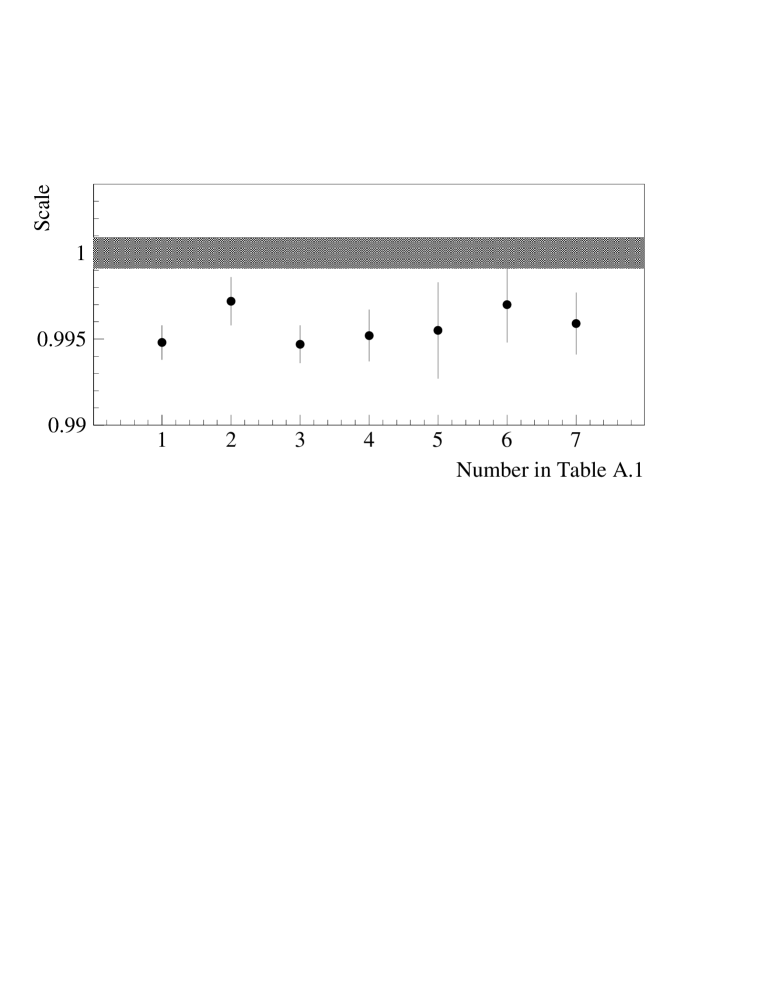
FIG. 56.: Required energy scales for various data samples. The shaded area represents the energy scale determined by the $Z\rightarrow\ e^{+}e^{-}$ mass.

2 Momentum Non-Linearity

A non-linearity in the $p_{T}$ measurement could produce a discrepancy between the two methods. The average $p_{T}$ of $\Upsilon$ ($\psi$) decay muons is $\sim 5.0$ GeV/c ($\sim 3.5$ GeV/c), while the average $p_{T}$ of W and Z decay electrons is $\sim 40$ GeV/c. Figure 14 shows the difference between the measured mass and the expected mass as a function of the sum of $1/p_{T}$ of the two muons in $\Upsilon$ and $\psi$ decays. $W$ and $Z$ events occur on the far left of the plot. No significant momentum non-linearity is observed.

3 Differences between the Electron and Muon Tracks

In the $E/p$ method, the electron momentum scale is determined from the muon momenta. In many ways, electron tracks are different from those of muons. They are produced with different internal bremsstrahlung. The external bremsstrahlung is also different, resulting in different momenta. Furthermore the external bremsstrahlung causes the tracks to have a non-zero impact parameter, which introduces a bias on the beam-constrained momentum. The simulation should take into account all the differences between electrons and muons, when the momentum scale determined by muons is transferred to the electron momentum. However, mishandling any of these differences in the simulation may cause a difference between the electron momentum scale and the muon momentum scale, causing a discrepancy between the $Z$ mass and $E/p$ methods. In principle, the electron momentum scale can be checked using electron tracks. However, as shown in Table XVI, the uncertainties are too large to allow us to have concrete conclusions.

This section describes the differences between electron tracks and muon tracks, how the simulation treats them, and the size of possible biases.

  Internal Bremsstrahlung Distribution:

“Internal” photons are photons which are produced at the vertex in a radiative $\mbox{$W\rightarrow\ e\nu$}\gamma$ event (or ${\mbox{$Z\rightarrow\ e^{+}e^{-}$}}\gamma$ event). For Monte Carlo events with no external photons, we find that the average $E/p$ between $0.9$ and $1.1$ is $1.0039$. Part of this shift above 1, 0.0014, is from cut biases, and the internal bremsstrahlung shifts the peak by 0.0025. The distribution we are using would have to be wrong by $\sim$100% for our fitted energy scale to come out shifted enough to account for the discrepancy between the energy scale from $M_{Z}$ and $E/p$.

• The generator that is used for $E/p$ simulation in these studies (PHOTOS [33] in two-photon mode) has been compared to the calculation by Berends and Kleiss of Reference [31], and the two generators give similar energy-angle distributions.

• Laporta and Odorico [50] argue that inclusion of multiple photon radiation from the final state electron may change the energy loss distribution of the electron relative to a single photon calculation, such as Berends and Kleiss. Reference [50] contains an algorithm to calculate the effect of a cascade of final state photons. By construction, this algorithm reduces to Berends and Kleiss for the case of single photon emission. Their algorithm is implemented for $W$ decays. The Laporta and Odorico case has the mean $E/p$ between $0.9$ and $1.1$ lower by $0.00033$. This is not insignificant, but it is not nearly large enough to account for the discrepancy between the $M_{Z}$ and $E/p$ methods. The statistical error on the Monte Carlo for this calculation is 0.00015.

• Baur, Keller, and Wackeroth [34] have done a calculation of the ${\mbox{$W\rightarrow\ e\nu$}\gamma}$ process which includes radiation from the $W$ propagator. We have received their calculation in the form of a Monte Carlo [51]. The Monte Carlo can implement their calculation, and it can also implement Berends and Kleiss. We run separately in each mode and implement some simple model of CEM clustering of the photons and measurement resolutions. We find that [34] produces a value for the mean of $E/p$ between $0.9$ and $1.1$ that is $0.00023$ lower than the Berends and Kleiss result.

  External Bremsstrahlung Distribution:

The formula we are using for the photon energy distribution was calculated in 1974 by Tsai [30]. This formula is still referenced in papers written today, but it is possible that the formula is unexpectedly breaking down at high energies. Evidence that it is not is given by the SLAC measurement of the Landau-Pomeranchuk-Migdal effect described below [52]. They measured the rate and energy distribution of bremsstrahlung of $25$ GeV electrons incident on different targets. For all the targets, they measured some level of bremsstrahlung suppression at low photon energies, as expected, but at higher photon energies, their measured distributions agreed well with the expectation from [30].

  Low Energy Bremsstrahlung Cutoff:

Since the number of external photons diverges as $1/E$, we only consider external photons above a certain energy. In particular, we only simulate photons above $y=0.1\%$, where $y$ is the fraction of the electron energy taken up by the photon. However, we can integrate the total fraction of the electron energy that is carried by photons below the cutoff. The total fraction is $y=0.1\%\times 0.085$, where $0.085$ is an approximation of the effective number of radiation lengths seen by the electrons, including the CTC gas and wires. We expect this to affect the energy scale by less than $0.0001$, which is a negligible amount. As a simple check we have increased the cutoff and we do not see any significant change in the fitted energy scale. A similar argument holds for the internal photons.

  Beam Constraint Biasing $E/p$:

The beam constraint can bias tracks that have undergone external radiation (bremsstrahlung) before the CTC active volume. Bremsstrahlung causes the tracks to have a non-zero impact parameter which biases the beam-constrained momentum. The simulation follows the same procedure, and so we expect this bias to be reproduced. Two possibilities are considered.

• The radial distribution of material may be wrong.
  The average radius of external radiation (including half the CTC gas) occurs at $22.21$ cm in the simulation. The bias depends on $r^{2}$, and so the location of the material might be sensitive to the scale. As a check the simulation is run with all the material before the CTC gas placed in the beampipe, or with all placed in the CTC inner can. The material is scaled so that $\langle X_{\circ}\rangle$ is the same for both cases. $f_{tail}$ for the beampipe case is higher than the CTC case by about $1\%$ of itself. The average $E/p$ from $0.9$ to $1.1$ is higher in the beampipe case than the CTC case by $0.0003$. Both of these changes are small. Considering that these are extreme cases for variations in the possible distributions of the material, the expected changes are negligible.

• In the simulation, the correlation between curvature and impact parameter mismeasurement may not be correct.
  This would cause the Monte Carlo to produce the wrong bias from the beam constraint. However, in the Monte Carlo, we use CTC wire hit patterns from the real $W$ data to derive a covariance matrix to use in the beam constraint. We use the identical procedure that is used to beam constraint the real data. The results are insensitive to the cuts on $D_{0}$ and to variations of the correlation.

We also try setting the energy scale with the $E/p$ distribution before the beam constraint. We compare the Monte Carlo distribution to the data distribution. We get a result for the energy scale which is consistent with the beam constrained $E/p$ result.

  Landau-Pomeranchuk-Migdal Effect.

Multiple scattering of the electron can suppress the production of bremsstrahlung at low photon energies [52]. Qualitatively, if the electron is disturbed while in the “formation zone” of the photon, the bremsstrahlung will be suppressed. The “formation zone” is appreciable for the low energy bremsstrahlung. (Similarly, the electron bending in a magnetic field can also suppress low energy photons, but the CDF magnet is not strong enough for this to be significant.) SLAC has measured this effect for $25$ GeV electrons. The suppression of bremsstrahlung depends on the density of the material and occurs below $y\simeq 0.01$ for gold and $y=0.001$ for carbon, where $y$ is the fraction of the electron energy taken up by the photon. The average density of material in the CDF detector before the CTC is closer to carbon than gold, and since we have a cutoff at $y=0.001$, we are in effect simulating $100\%$ suppression for the carbon case. This is a negligible effect on $E/p$. Any effect, if there were, will make the discrepancy bigger.

  Synchrotron Radiation.

We considered the possibility that secondary particles, such as synchrotron photons, may interact in the drift chamber, generating spurious hits and biasing the electron momentum measurement. To estimate the effect of synchrotron photons, we used a simple Monte Carlo simulation to convolute the synchrotron radiation spectrum for 35 GeV electrons with the photoelectric absorption length in argon/ethane. Assuming each absorbed photon to produce one drift chamber hit (except for the merging of nearby hits due to finite pulse widths), electron and photo-electron hits were fed to a hit-level drift chamber simulation and processed by the full track reconstruction software. The predicted bias in beam-constrained momenta due to synchrotron photons was $\sim-0.02\%$, more than an order of magnitude too small to explain the energy scale discrepancy. We performed a second study, using a GEANT-based detector simulation under development for a future run of the CDF experiment. We used GEANT to simulate secondary particles near a 35 GeV electron, using the material distribution of the upgraded detector, and transplanted the secondaries into the same hit-level simulation used in the first study. The bias due to secondary particles was again $\sim-0.02\%$. We conclude that interactions of secondary particles in the drift chamber are unlikely to be the source of the discrepancy.

  Significant Energy Loss in Silicon Crystals.

An electron moving through the material before the CTC will pass through $\approx 400~{}\mu$m of aligned silicon crystals. If it travels through the crystal along a major axis of symmetry, it can potentially lose significantly more energy than is lost through bremsstrahlung [53]. However, in the data we do not see any significant difference between electrons that pass through the SVX^′ and those that do not, relative to the Monte Carlo. This indicates that this is not a significant effect.

  Track Quality Comparison.

In a completely data-driven study, we examined a large number of track quality variables, such as hit residuals signed in various ways, track $\chi^{2}$, and correlations between hit residuals, as well as occupancies and pulse widths. While we had no quantitative model in mind to set the scale for comparisons, none of the track variables we considered showed any significant difference between the $W$ electron and $W$ muon samples.

4 Other Checks

  Invariant Mass Measurement:

Calculating the invariant mass of $Z\rightarrow\ e^{+}e^{-}$ events makes use of a different set of track parameters than calculating $E/p$, and one could hypothesize errors in the angular variables causing errors in the invariant mass. We would not necessarily expect the electron and muon invariant masses to look the same since one uses $E_{T}$ and the other $p_{T}$. One could also imagine measurement correlations between the different tracking parameters which have the net effect of shifting the measured mass. The two tracks themselves could also be correlated since for $Z$ events they are largely back-to-back. For example, if one track enters a superlayer on the right side of a cell, the other track will be biased to do the same. However, we have not been able to see any effect on the $Z$ mass in the data.

  Inner Superlayers:

Wires of the CTC inner superlayers have larger occupancy than those of the outer superlayers, giving a higher probability of using wrong hits in the inner layers. To check this the $Z$ electron tracks are refit with superlayers 0 and 1 removed. While the resolution becomes worse, no significant change is seen in the means of $E/p$ of the electrons or the invariant mass of $Z$ electron tracks. Refitting is also done with the same tracks but by removing superlayer 5 instead of 0 and 1. Again no significant change was observed in the means of $E/p$, or the invariant mass of $Z$ electron tracks. The mean of the $E/p$ distribution of $W$ data is checked with the number of stereo or axial hits used in the track reconstruction. It is found to be insensitive to the number of hits.

  Coding Errors.

Several independent $E/p$ simulation codes produce highly consistent results.

  CEM Non-Linearity.

When we applied the non-linearity correction of Section IV E, the CEM energy scale factor as determined from $E/p$ moved from $0.9963$ to $0.9948$, which makes the discrepancy between $E/p$ and $M_{Z}$ worse. The uncertainty on the energy scale was also significantly increased by the uncertainty on the non-linearity. If we do not consider a non-linearity correction, then the discrepancy between the Z mass energy scale and the $E/p$ energy scale is closer to $3.3$ standard deviations. The data (see Figure 18), however, support a CEM non-linearity.

  Amount of Material is Incorrect.

To increase the fitted energy scale by $0.5$ %, we would have to increase the amount of material in the Monte Carlo by $\sim 5.6$ % of a radiation length. However, the tail of the $E/p$ distribution of the $W$ data is not consistent with such an increase. Moreover, the low tail of the invariant mass distribution of $J/\psi\rightarrow\mbox{$e^{+}e^{-}$}$ decays (see Figure 55) has been examined, and such an increase in the amount of material would significantly contradict the data.

  Backgrounds are Biasing the Result.

It is possible that our estimate of the $E/p$ shape of the background is flawed, and that there is a significant source of non-electron background in the $E/p$ peak region that is biasing our energy scale fit. We consider the worst case possibility that all the background is located at one of the edges of the $E/p$ fit region. To increase the $S_{E}(E/p)$ to 1, we would need to have about $6\%$ background piled up at $E/p=1.1$. This is a factor of $\sim$17 larger than the QCD background we have measured, and since we expect the QCD background to be largely flat in $E/p$, we do not expect that backgrounds are significantly biasing our result. The agreement of the $Z$ $E/p$ fit with the $W$ fit also indicates that the backgrounds are not a significant effect in the $W$ fit.

  Tracking Resolutions Not Simulated Correctly.

For the Monte Carlo, we smear the track parameters according to the calculated covariance matrix, and we then apply the beam constraint according to this same covariance matrix. Thus, in the Monte Carlo, the covariance matrix used in the beam constraint describes the correlations and resolutions of the track parameters exactly. On the other hand, it is not necessarily the case for the data that the correlations and resolutions are described correctly by the covariance matrix.

We can measure the correlation between impact parameter and curvature by plotting the average of $qD_{0}$ as a function of $E/p$. The slope of this plot for the data is slightly different than for the Monte Carlo. Since the Monte Carlo covariance matrix is the same matrix that is used to beam constrain the data, we conclude that the beam constraint covariance matrix does not perfectly describe the underlying measurement correlations of the data.

To see how much of an effect this has on $E/p$ we run the Monte Carlo as follows: We smear the Monte Carlo according to an adjusted covariance matrix, where all the off-diagonal terms are set to $0$ except for $\sigma^{2}(C,D_{0})$, and which we fix according to the $W$ data. When we apply the beam constraint, however, we use the same covariance matrices that are used by the data to do the beam constraint. In this way, we simulate the data more closely: smearing according to one matrix, and beam constraining according to a slightly different matrix. We find no effect on the average $E/p$ between $0.9$ and $1.1$.

  The Solenoid May Cause Non-Linearity in Photon Response.

The solenoid coil presents $\sim 1$ radiation length for electrons in $W$ and $Z$ events, and also for any associated soft photons. Electron energy losses in the solenoid are not expected to affect our results since they are part of the CEM scale, which we are fitting for. However, it is possible that the soft photons are not making it through the solenoid and that this is distorting the $E/p$ shape. As a simple check, we use a formula from the PDG Full Listings [29] which describes the energy loss profile of a particle as a function of its depth in radiation lengths. We apply this formula to all the photons created in the Monte Carlo and reduce their energy accordingly. This is not a rigorous check since we are applying the formula to low energy photons, which are in an energy region where the formula is not necessarily accurate. We rerun the $Z$ Monte Carlo with this effect put in, and we treat this new Monte Carlo as “data” and fit it with the default Monte Carlo. Fitting $E/p$ gives a Monte Carlo energy scale of $0.99960$, and fitting $M_{Z}$ gives a scale of $0.99935$. We are interested in $M_{Z}$ relative to $E/p$, and thus $0.99960-0.99935=0.00025\pm 0.00015$. This is more than an order of magnitude too small to explain the energy scale discrepancy.

5 Conclusion

We have measured the energy scale using the peak of the $E/p$ distribution of $W$ data. The $E/p$ distribution of $Z$ events gives consistent results for the $E/p$ distribution of $W$ events. However, if we set the energy scale with $E/p$, then the invariant mass distribution of the $Z$ events comes out significantly low. As a check we have refit the Run IA data with the Run IB Monte Carlo simulation, and the result agrees excellently with the published results.

We have discussed several possible reasons that the $Z$ mass comes out wrong. The problem could be a momentum scale problem or otherwise a tracking problem; it could be related to our simulation of $E/p$ as presented in this paper; or it could be something theoretically unexpected. None of the plausible explanations considered here appears to be capable of creating a discrepancy of the magnitude observed in the Run IB data sample, and the source for the inconsistency remains an open question.

For the final $W$ mass measurement reported in this paper, we have used the invariant mass of the $Z\rightarrow\ e^{+}e^{-}$ and $Z\rightarrow\mu^{+}\mu^{-}$ events. In this way, we have separated our energy scale measurement from almost all questions associated with the $E/p$ method.

REFERENCES

- [1] S. L. Glashow, Nucl. Phys. 22, 579 (1961); S. Weinberg, Phys. Rev. Lett. 19, 1264 (1967); A. Salam, Proceedings of the Eighth Nobel Symposium, edited by N. Svartholm (Almqvist and Wiksells, Stockholm, Wiley, New York, 1968), p. 367.
- [2] C. Caso et al. (Particle Data Group), Eur. Phys. J. C3, 90 (1998).
- [3] J. Alitti et al. (UA2 Collaboration), Phys. Lett. B276, 354 (1992).
- [4] F. Abe et al. (CDF Collaboration), Phys. Rev. Lett. 75, 11 (1995); F. Abe et al. (CDF Collaboration), Phys. Rev. D52, 1784 (1995).
- [5] B. Abbott et al. (DO/ Collaboration), Phys. Rev. Lett. 84, 222 (2000); B. Abbott et al. (DO/ Collaboration), Phys. Rev. Lett. 80, 3008 (1998); B. Abbott et al. (DO/ Collaboration), Phys. Rev. D58, 092003 (1998).
- [6] R. Barate et al. (ALEPH Collaboration), Phys. Lett. B401, 347 (1997); P. Abreu et al. (DELPHI Collaboration), Phys. Lett. B397, 158 (1997); M. Acciarri et al. (L3 Collaboration), Phys. Lett. B398, 223, (1997); G. Abbiendi et al. (OPAL Collaboration), Phys. Lett. B389, 384 (1996).
- [7] R. Barate et al. (ALEPH Collaboration), Eur. Phys. J. C17, 241 (2000) and Phys. Lett. B453, 121 (1999); P. Abreu et al. (DELPHI Collaboration), Phys. Lett. B462, 410 (1999); M. Acciarri et al. (L3 Collaboration), Phys. Lett. B454, 386 (1999); G. Abbiendi et al. (OPAL Collaboration), hep-ex/0009018 and Phys. Lett. B453, 138 (1999).
- [8] This average includes the LEP II measurements upto = 183 GeV. Thus the ALEPH’s published measurement at = 189 GeV and the OPAL’s preliminary measurement at = 189 GeV are not included.
- [9] LEP and SLD Collaborations, CERN-EP-2000-16 (unpublished), see http://www.cern.ch/LEPEWWG/.
- [10] G. P. Zeller et al. (NuTeV Collaboration), for proc. DPF 99, Los Angeles, CA (1999), hep-ex/9906024.
- [11] F. Abe et al. (CDF Collaboration), hep-ex/0006028 (submitted to Phys. Rev. D); F. Abe et al. (CDF Collaboration), Phys. Rev. Lett., 82, 271 (1999); B. Abbott et al. (DO/ Collaboration), Phys. Rev., D58, 052001 (1998).
- [12] F. Abe et al. (CDF Collaboration), Phys. Rev. Lett. 65, 2243 (1990); F. Abe et al. (CDF Collaboration), Phys. Rev. D43, 2070 (1991).
- [13] S. D. Drell and T.-M. Yan, Phys. Rev. Lett. 25, 316 (1970); for QCD resummation see C. Balaza and C.-P. Yuan, Phys. Rev. D56, 5558 (1997); R. K. Ellis and S. Veseli, Nucl. Phys. B511, 649 (1998).
- [14] F. Abe et al. (CDF Collaboration), Nucl. Instr. and Meth. A271, 387 (1988).
- [15] F. Abe et al. (CDF Collaboration), Phys. Rev. D50, 2966 (1994).
- [16] D. Amidei et al., Nucl. Instr. and Meth. A350, 73 (1994); P. Azzi et al., Nucl. Instr. and Meth. A360, 137 (1995).
- [17] F. Snider et al., Nucl. Instr. and Meth. A268, 75 (1988). This is the reference for the previous generation of the device. The replacement for the 1992-93 datataking period has more modules of a shorter drift length, but is otherwise similar.
- [18] F. Bedeschi et al., Nucl. Instr. and Meth. A268, 50 (1988).
- [19] L. Balka et al., Nucl. Instr. and Meth. A267, 272 (1988); S. R. Hahn et al., Nucl. Instr. and Meth. A267, 351 (1988); K. Yasuoka et al., Nucl. Instr. and Meth. A267, 315 (1988); R. G. Wagner et al., Nucl. Instr. and Meth. A267, 330 (1988); T. Devlin et al., Nucl. Instr. and Meth. A267, 24 (1988).
- [20] S. Bertolucci et al., Nucl. Instr. and Meth. A267, 301 (1988).
- [21] Y. Fukui et al., Nucl. Instr. and Meth. A267, 280 (1988); W. C. Carithers et al., “Proceedings of the Gas Sampling Calorimetry Workshop II,” Batavia, Illinois, 54 (1985). S. Cihangir et al., Nucl. Instr. and Meth. A267, 249 (1988); G. Brandenburg et al., Nucl. Instr. and Meth. A267, 257 (1988).
- [22] G. Ascoli et al., Nucl. Instr. and Meth. A268, 33 (1988); G. Ascoli et al., Nucl. Instr. and Meth. A268, 41 (1988).
- [23] D. Amidei et al., Nucl. Instr. and Meth. A269, 51 (1988).
- [24] T. Carroll et al., Nucl. Instr. and Meth. A263, 199 (1988).
- [25] G. W. Foster et al., Nucl. Instr. and Meth. A269, 93 (1988).
- [26] K. Byrum et al., Nucl. Instr. and Meth. A364, 144 (1995).
- [27] F. Abe et al. (CDF Collaboration), Phys. Rev Lett. 63, 720 (1989).
- [28] A. Gordon, Ph.D. Thesis, Harvard University, 1998.
- [29] Particle Data Group, Eur. Phys. J. C3, 1 (1998).
- [30] Y.-S. Tsai, Rev. Mod. Phys. 45, 815 (1974).
- [31] F. A. Berends and R. Kleiss, J.P. Reval, J.P. Vialle, Z. Phys. C27, 155 (1985); F. A. Berends and R. Kleiss, Z. Phys. C27, 365 (1985).
- [32] R. G. Wagner, Comput. Phys. Commun. 70, 15 (1992).
- [33] E. Barberio, Z. Was, Comput. Phys. Comm. 79, 291 (1994); E. Barberio, B. van Eijk, Z. Was, Comput. Phys. Comm. 66, 115 (1991).
- [34] U. Baur, S. Keller, D. Wackeroth, Phys. Rev. D59, 013992 (1999).
- [35] A.D. Martin, W.J. Stirling, R.G. Roberts, MRS-R2.
-
[36]
F. Abe et al. (CDF Collaboration),
Phys. Rev. Lett. 81, 5754 (1998).
The forward/backward charge asymmetry in decays is defined as: where is the cross section for decays as a function of lepton pseudorapidity, . - [37] A.D. Martin et al., Eur. Phys. J. C4, 463 (1998).
- [38] CTEQ-5 PDFs, the CTEQ collaboration. Pre-release obtained.
- [39] W. Giele et al., Nucl. Phys. B403, 633 (1993).
- [40] “Parton Distributions, d/u, and Higher Twists at High ”, U.K. Yang, A. Bodek and Q. Fan, Proceedings of the Rencontres de Moriond: QCD and High-energy Hadronic Interactions, Les Arcs, France, April 1998 and UR-1518 (1998).
- [41] A. Arneodo et al., NMC Collaboration, Nucl. Phys. B487, 3 (1997).
- [42] M. H. Reno, University of Iowa preprint UIOWA-94-01, 1994.
- [43] G.A. Ladinsky, C.-P. Yuan, Phys. Rev. D50, 4239 (1994).
- [44] R.K. Ellis, S. Veseli, Nucl. Phys. B511, 649 (1998); R.K. Ellis, D.A. Ross, S. Veseli, Nucl. Phys. B503, 309 (1997).
- [45] E. Mirkes, Nucl. Phys. B387, 3 (1992).
- [46] J. Collins and D. Soper, Phys. Rev. D16, 2219 (1977).
- [47] Jonathan LO. Rosner and Mihir P. Worah, Phys. Rev. D49, 1363 (1994).
- [48] T. Affolder et al. (CDF Collaboration), submitted to PRL (2000).
- [49] M. Swartz, hep-ph/9509248; S. Eidelman, F. Jegerlehner, hep-ph/9502298
- [50] S. Laporta and R. Odorico, Nucl. Phys. B266, 633 (1986).
- [51] U. Baur, personal communication.
- [52] P.L. Anthony et al., Phys. Rev. Lett. 75, 1949 (1995).
- [53] V.N. Baier, V.M. Katkov, and V.M. Strakhovenko, Nucl. Inst. and Meth. B16, 5 (1986); V.N. Baier, V.M. Katkov, and V.M. Strakhovenko, Sov. Phys. JETP 65, 4 (1987).