EUROPEAN ORGANIZATION FOR NUCLEAR RESEARCH

CERN-EP-2000-092

July 7, 2000

Two Higgs Doublet Model and Model Independent
Interpretation of Neutral Higgs Boson Searches

The OPAL Collaboration

Abstract

Searches for the neutral Higgs bosons $\mathrm{h}^{0}$ and $\mathrm{A}^{0}$  are used to obtain limits on the Type II Two Higgs Doublet Model (2HDM(II)) with no CP–violation in the Higgs sector and no additional particles besides the five Higgs bosons. The analysis combines approximately 170 pb^-1 of data collected with the OPAL detector at $\sqrt{s}\approx 189$ GeV with previous runs at $\sqrt{s}\approx m_{Z}$ and $\sqrt{s}\approx 183$ GeV. The searches are sensitive to the $\mathrm{h}^{0}$, $\mathrm{A}^{0}$$\rightarrow$$\mathrm{q}\bar{\mathrm{q}}$, $\mathrm{g}\mathrm{g}$, $\tau^{+}\tau^{-}$ and $\mathrm{h}^{0}$$\rightarrow$$\mathrm{A}^{0}$$\mathrm{A}^{0}$ decay modes of the Higgs bosons. For the first time, the 2HDM(II) parameter space is explored in a detailed scan, and new flavour independent analyses are applied to examine regions in which the neutral Higgs bosons decay predominantly into light quarks or gluons. Model–independent limits are also given.

(Submitted to European Physical Journal C)

The OPAL Collaboration

G. Abbiendi², K. Ackerstaff⁸, C. Ainsley⁵, P.F. Åkesson³, G. Alexander²², J. Allison¹⁶, K.J. Anderson⁹, S. Arcelli¹⁷, S. Asai²³, S.F. Ashby¹, D. Axen²⁷, G. Azuelos^18,a, I. Bailey²⁶, A.H. Ball⁸, E. Barberio⁸, R.J. Barlow¹⁶, S. Baumann³, T. Behnke²⁵, K.W. Bell²⁰, G. Bella²², A. Bellerive⁹, G. Benelli², S. Bentvelsen⁸, S. Bethke³², O. Biebel³², I.J. Bloodworth¹, O. Boeriu¹⁰, P. Bock¹¹, J. Böhme^14,h, D. Bonacorsi², M. Boutemeur³¹, S. Braibant⁸, P. Bright-Thomas¹, L. Brigliadori², R.M. Brown²⁰, H.J. Burckhart⁸, J. Cammin³, P. Capiluppi², R.K. Carnegie⁶, A.A. Carter¹³, J.R. Carter⁵, C.Y. Chang¹⁷, D.G. Charlton^1,b, P.E.L. Clarke¹⁵, E. Clay¹⁵, I. Cohen²², O.C. Cooke⁸, J. Couchman¹⁵, C. Couyoumtzelis¹³, R.L. Coxe⁹, A. Csilling^15,j, M. Cuffiani², S. Dado²¹, G.M. Dallavalle², S. Dallison¹⁶, A. de Roeck⁸, E. de Wolf⁸, P. Dervan¹⁵, K. Desch²⁵, B. Dienes^30,h, M.S. Dixit⁷, M. Donkers⁶, J. Dubbert³¹, E. Duchovni²⁴, G. Duckeck³¹, I.P. Duerdoth¹⁶, P.G. Estabrooks⁶, E. Etzion²², F. Fabbri², M. Fanti², L. Feld¹⁰, P. Ferrari¹², F. Fiedler⁸, I. Fleck¹⁰, M. Ford⁵, A. Frey⁸, A. Fürtjes⁸, D.I. Futyan¹⁶, P. Gagnon¹², J.W. Gary⁴, G. Gaycken²⁵, C. Geich-Gimbel³, G. Giacomelli², P. Giacomelli⁸, D. Glenzinski⁹, J. Goldberg²¹, C. Grandi², K. Graham²⁶, E. Gross²⁴, J. Grunhaus²², M. Gruwé²⁵, P.O. Günther³, C. Hajdu²⁹, G.G. Hanson¹², M. Hansroul⁸, M. Hapke¹³, K. Harder²⁵, A. Harel²¹, M. Harin-Dirac⁴, A. Hauke³, M. Hauschild⁸, C.M. Hawkes¹, R. Hawkings⁸, R.J. Hemingway⁶, C. Hensel²⁵, G. Herten¹⁰, R.D. Heuer²⁵, J.C. Hill⁵, A. Hocker⁹, K. Hoffman⁸, R.J. Homer¹, A.K. Honma⁸, D. Horváth^29,c, K.R. Hossain²⁸, R. Howard²⁷, P. Hüntemeyer²⁵, P. Igo-Kemenes¹¹, K. Ishii²³, F.R. Jacob²⁰, A. Jawahery¹⁷, H. Jeremie¹⁸, C.R. Jones⁵, P. Jovanovic¹, T.R. Junk⁶, N. Kanaya²³, J. Kanzaki²³, G. Karapetian¹⁸, D. Karlen⁶, V. Kartvelishvili¹⁶, K. Kawagoe²³, T. Kawamoto²³, R.K. Keeler²⁶, R.G. Kellogg¹⁷, B.W. Kennedy²⁰, D.H. Kim¹⁹, K. Klein¹¹, A. Klier²⁴, S. Kluth³², T. Kobayashi²³, M. Kobel³, T.P. Kokott³, S. Komamiya²³, R.V. Kowalewski²⁶, T. Kress⁴, P. Krieger⁶, J. von Krogh¹¹, T. Kuhl³, M. Kupper²⁴, P. Kyberd¹³, G.D. Lafferty¹⁶, H. Landsman²¹, D. Lanske¹⁴, I. Lawson²⁶, J.G. Layter⁴, A. Leins³¹, D. Lellouch²⁴, J. Letts¹², L. Levinson²⁴, R. Liebisch¹¹, J. Lillich¹⁰, B. List⁸, C. Littlewood⁵, A.W. Lloyd¹, S.L. Lloyd¹³, F.K. Loebinger¹⁶, G.D. Long²⁶, M.J. Losty⁷, J. Lu²⁷, J. Ludwig¹⁰, A. Macchiolo¹⁸, A. Macpherson^28,m, W. Mader³, S. Marcellini², T.E. Marchant¹⁶, A.J. Martin¹³, J.P. Martin¹⁸, G. Martinez¹⁷, T. Mashimo²³, P. Mättig²⁴, W.J. McDonald²⁸, J. McKenna²⁷, T.J. McMahon¹, R.A. McPherson²⁶, F. Meijers⁸, P. Mendez-Lorenzo³¹, W. Menges²⁵, F.S. Merritt⁹, H. Mes⁷, A. Michelini², S. Mihara²³, G. Mikenberg²⁴, D.J. Miller¹⁵, W. Mohr¹⁰, A. Montanari², T. Mori²³, K. Nagai⁸, I. Nakamura²³, H.A. Neal^12,f, R. Nisius⁸, S.W. O’Neale¹, F.G. Oakham⁷, F. Odorici², H.O. Ogren¹², A. Oh⁸, A. Okpara¹¹, M.J. Oreglia⁹, S. Orito²³, G. Pásztor^8,j, J.R. Pater¹⁶, G.N. Patrick²⁰, J. Patt¹⁰, P. Pfeifenschneider^14,i, J.E. Pilcher⁹, J. Pinfold²⁸, D.E. Plane⁸, B. Poli², J. Polok⁸, O. Pooth⁸, M. Przybycień^8,d, A. Quadt⁸, C. Rembser⁸, P. Renkel²⁴, H. Rick⁴, N. Rodning²⁸, J.M. Roney²⁶, S. Rosati³, K. Roscoe¹⁶, A.M. Rossi², Y. Rozen²¹, K. Runge¹⁰, O. Runolfsson⁸, D.R. Rust¹², K. Sachs⁶, T. Saeki²³, O. Sahr³¹, E.K.G. Sarkisyan²², C. Sbarra²⁶, A.D. Schaile³¹, O. Schaile³¹, P. Scharff-Hansen⁸, M. Schröder⁸, M. Schumacher²⁵, C. Schwick⁸, W.G. Scott²⁰, R. Seuster^14,h, T.G. Shears^8,k, B.C. Shen⁴, C.H. Shepherd-Themistocleous⁵, P. Sherwood¹⁵, G.P. Siroli², A. Skuja¹⁷, A.M. Smith⁸, G.A. Snow¹⁷, R. Sobie²⁶, S. Söldner-Rembold^10,e, S. Spagnolo²⁰, M. Sproston²⁰, A. Stahl³, K. Stephens¹⁶, K. Stoll¹⁰, D. Strom¹⁹, R. Ströhmer³¹, L. Stumpf²⁶, B. Surrow⁸, S.D. Talbot¹, S. Tarem²¹, R.J. Taylor¹⁵, R. Teuscher⁹, M. Thiergen¹⁰, J. Thomas¹⁵, M.A. Thomson⁸, E. Torrence⁹, S. Towers⁶, D. Toya²³, T. Trefzger³¹, I. Trigger⁸, Z. Trócsányi^30,g, E. Tsur²², M.F. Turner-Watson¹, I. Ueda²³, B. Vachon${26}$, P. Vannerem¹⁰, M. Verzocchi⁸, H. Voss⁸, J. Vossebeld⁸, D. Waller⁶, C.P. Ward⁵, D.R. Ward⁵, P.M. Watkins¹, A.T. Watson¹, N.K. Watson¹, P.S. Wells⁸, T. Wengler⁸, N. Wermes³, D. Wetterling¹¹ J.S. White⁶, G.W. Wilson¹⁶, J.A. Wilson¹, T.R. Wyatt¹⁶, S. Yamashita²³, V. Zacek¹⁸, D. Zer-Zion^8,l

¹School of Physics and Astronomy, University of Birmingham, Birmingham B15 2TT, UK
²Dipartimento di Fisica dell’ Università di Bologna and INFN, I-40126 Bologna, Italy
³Physikalisches Institut, Universität Bonn, D-53115 Bonn, Germany
⁴Department of Physics, University of California, Riverside CA 92521, USA
⁵Cavendish Laboratory, Cambridge CB3 0HE, UK
⁶Ottawa-Carleton Institute for Physics, Department of Physics, Carleton University, Ottawa, Ontario K1S 5B6, Canada
⁷Centre for Research in Particle Physics, Carleton University, Ottawa, Ontario K1S 5B6, Canada
⁸CERN, European Organisation for Nuclear Research, CH-1211 Geneva 23, Switzerland
⁹Enrico Fermi Institute and Department of Physics, University of Chicago, Chicago IL 60637, USA
¹⁰Fakultät für Physik, Albert Ludwigs Universität, D-79104 Freiburg, Germany
¹¹Physikalisches Institut, Universität Heidelberg, D-69120 Heidelberg, Germany
¹²Indiana University, Department of Physics, Swain Hall West 117, Bloomington IN 47405, USA
¹³Queen Mary and Westfield College, University of London, London E1 4NS, UK
¹⁴Technische Hochschule Aachen, III Physikalisches Institut, Sommerfeldstrasse 26-28, D-52056 Aachen, Germany
¹⁵University College London, London WC1E 6BT, UK
¹⁶Department of Physics, Schuster Laboratory, The University, Manchester M13 9PL, UK
¹⁷Department of Physics, University of Maryland, College Park, MD 20742, USA
¹⁸Laboratoire de Physique Nucléaire, Université de Montréal, Montréal, Quebec H3C 3J7, Canada
¹⁹University of Oregon, Department of Physics, Eugene OR 97403, USA
²⁰CLRC Rutherford Appleton Laboratory, Chilton, Didcot, Oxfordshire OX11 0QX, UK
²¹Department of Physics, Technion-Israel Institute of Technology, Haifa 32000, Israel
²²Department of Physics and Astronomy, Tel Aviv University, Tel Aviv 69978, Israel
²³International Centre for Elementary Particle Physics and Department of Physics, University of Tokyo, Tokyo 113-0033, and Kobe University, Kobe 657-8501, Japan
²⁴Particle Physics Department, Weizmann Institute of Science, Rehovot 76100, Israel
²⁵Universität Hamburg/DESY, II Institut für Experimental Physik, Notkestrasse 85, D-22607 Hamburg, Germany
²⁶University of Victoria, Department of Physics, P O Box 3055, Victoria BC V8W 3P6, Canada
²⁷University of British Columbia, Department of Physics, Vancouver BC V6T 1Z1, Canada
²⁸University of Alberta, Department of Physics, Edmonton AB T6G 2J1, Canada
²⁹Research Institute for Particle and Nuclear Physics, H-1525 Budapest, P O Box 49, Hungary
³⁰Institute of Nuclear Research, H-4001 Debrecen, P O Box 51, Hungary
³¹Ludwigs-Maximilians-Universität München, Sektion Physik, Am Coulombwall 1, D-85748 Garching, Germany
³²Max-Planck-Institute für Physik, Föhring Ring 6, 80805 München, Germany

^a and at TRIUMF, Vancouver, Canada V6T 2A3
^b and Royal Society University Research Fellow
^c and Institute of Nuclear Research, Debrecen, Hungary
^d and University of Mining and Metallurgy, Cracow
^e and Heisenberg Fellow
^f now at Yale University, Dept of Physics, New Haven, USA
^g and Department of Experimental Physics, Lajos Kossuth University, Debrecen, Hungary
^h and MPI München
ⁱ now at MPI für Physik, 80805 München
^j and Research Institute for Particle and Nuclear Physics, Budapest, Hungary
^k now at University of Liverpool, Dept of Physics, Liverpool L69 3BX, UK
^l and University of California, Riverside, High Energy Physics Group, CA 92521, USA
^m and CERN, EP Div, 1211 Geneva 23.

1 Introduction

In this study approximately 170 $\mathrm{pb}^{-1}$ of the data collected by the OPAL detector at LEP at $189$ GeV centre-of-mass energy are combined with 58 $\mathrm{pb}^{-1}$ of data taken at the $\mathrm{Z}^{0}$ pole and 53 $\mathrm{pb}^{-1}$ of data at $\sqrt{s}$ $\approx$ 183 GeV to search for neutral Higgs bosons [1, 2, 3] in the framework of the Type II Two Higgs Doublet Model with no CP–violation in the Higgs sector and no additional particles besides those arising from the Higgs mechanism (2HDM(II)) [4, 5]. A model–independent scheme, in which no assumption is made on the structure of the Higgs sector, is also analysed.

In the minimal Standard Model (SM) the Higgs sector comprises only one complex Higgs doublet [1] resulting in one physical neutral Higgs scalar whose mass is a free parameter of the theory. However, since there is no experimental evidence for the Higgs boson, it is important to study extended models containing more than one physical Higgs boson in the spectrum. In particular, Two Higgs Doublet Models (2HDMs) are attractive extensions of the SM since they add new phenomena with the fewest new parameters; they satisfy the constraints of $\rho\approx 1$ and the absence of tree-level flavour changing neutral currents, if the Higgs-fermion couplings are appropriately chosen. In the context of 2HDMs the Higgs sector comprises five physical Higgs bosons: two neutral CP-even scalars, $\mathrm{h}^{0}$ and $\mathrm{H}^{0}$ (with $m_{\mathrm{h}}$ $<$ $m_{\mathrm{H}}$), one CP-odd scalar, $\mathrm{A}^{0}$, and two charged scalars, $\mathrm{H}^{\pm}$.

The most general CP–invariant Higgs potential, having two complex $Y=1$, $SU(2)_{L}$ doublet scalar fields $\phi_{1}$ and $\phi_{2}$, is given by [4, 5, 6]

$${{V(\phi_{1},\phi_{2})}}={\kappa_{1}}(\phi_{1}^{\dagger}\phi_{1}-{v_{1}^{2}})^{2}+{\kappa_{2}}(\phi_{2}^{\dagger}\phi_{2}-{v_{2}^{2}})^{2}+{\kappa_{3}}[(\phi_{1}^{\dagger}\phi_{1}-{v_{1}^{2}})+(\phi_{2}^{\dagger}\phi_{2}-{v_{2}^{2}})]^{2}$$

$$+{\kappa_{4}}[(\phi_{1}^{\dagger}\phi_{1})(\phi_{2}^{\dagger}\phi_{2})-(\phi_{1}^{\dagger}\phi_{2})(\phi_{2}^{\dagger}\phi_{1})]+{\kappa_{5}}[{\mathrm{Re}}(\phi_{1}^{\dagger}\phi_{2})-v_{1}v_{2}]^{2}+{\kappa_{6}}[{\mathrm{Im}}(\phi_{1}^{\dagger}\phi_{2})]^{2},$$ (1)

where the vacuum expectation values, $v_{i}$, are non–negative real parameters and the couplings, $\kappa_{i}$, are real parameters. The physical masses at tree level are given by:

$$m^{2}_{{\mathrm{H,h}}}=\frac{1}{2}[{\mathcal{M}}_{11}+{\mathcal{M}}_{22}\pm\sqrt{({\mathcal{M}}_{11}-{\mathcal{M}}_{22})^{2}+4{\mathcal{M}}^{2}_{12}}],$$ (2)

$$m_{\mathrm{A}}^{2}=\kappa_{6}(v_{1}^{2}+v_{2}^{2}),~{}~{}~{}m_{\mathrm{H}^{\pm}}^{2}=\kappa_{4}(v_{1}^{2}+v_{2}^{2}),$$ (3)

where

$${\mathcal{M}}_{11}=4(\kappa_{1}+\kappa_{3})v_{1}^{2}+\kappa_{5}v_{2}^{2}$$ (4)

$${\mathcal{M}}_{22}=4(\kappa_{2}+\kappa_{3})v_{2}^{2}+\kappa_{5}v_{1}^{2}$$ (5)

$${\mathcal{M}}_{12}=(4\kappa_{3}+\kappa_{5})v_{1}v_{2}.$$ (6)

The Higgs mixing angle, $\alpha$, is obtained from

$$\cos{2\alpha}=\frac{{\mathcal{M}}_{11}-{\mathcal{M}}_{22}}{\sqrt{({\mathcal{M}}_{11}-{\mathcal{M}}_{22})^{2}+4{\mathcal{M}}_{12}^{2}}},$$ (7)

$$\sin{2\alpha}=\frac{2{\mathcal{M}}_{12}}{\sqrt{({\mathcal{M}}_{11}-{\mathcal{M}}_{22})^{2}+4{\mathcal{M}}_{12}^{2}}},$$ (8)

and the angle $\beta$ is defined as the ratio of the vacuum expectation values, $v_{1}$ and $v_{2}$, of the two scalar fields, $\mbox{$\tan\!\beta$}=v_{2}/v_{1}$, with $0\leq\beta\leq\pi/2$.

At the centre-of-mass energies accessed by LEP, the $\mathrm{h}^{0}$ and $\mathrm{A}^{0}$ bosons are expected to be produced predominantly via two processes: the Higgs–strahlung process ${\mathrm{e}}^{+}{\mathrm{e}}^{-}$$\rightarrow$$\mathrm{h}^{0}$$\mathrm{Z}^{0}$ and the pair–production process ${\mathrm{e}}^{+}{\mathrm{e}}^{-}$$\rightarrow$$\mathrm{h}^{0}$$\mathrm{A}^{0}$. The cross-sections for these two processes, $\sigma_{\mathrm{hZ}}$ and $\sigma_{\mathrm{hA}}$, are related at tree-level to the SM cross-sections by the following relations [6]:

$$\mbox{${\mathrm{e}}^{+}{\mathrm{e}}^{-}$}\mbox{$\rightarrow$}\mbox{$\mathrm{h}^{0}$}\mbox{$\mathrm{Z}^{0}$}\;: \sigma_{\mathrm{hZ}}=\sin^{2}(\beta-\alpha)~{}\sigma^{\mathrm{SM}}_{\mathrm{HZ}},$$ (9)

$$\mbox{${\mathrm{e}}^{+}{\mathrm{e}}^{-}$}\mbox{$\rightarrow$}\mbox{$\mathrm{h}^{0}$}\mbox{$\mathrm{A}^{0}$}\;: \sigma_{\mathrm{hA}}=\cos^{2}(\beta-\alpha)~{}\bar{\lambda}~{}\sigma^{\mathrm{SM}}_{\mathrm{HZ}},$$ (10)

where $\sigma^{\mathrm{SM}}_{\mathrm{HZ}}$ is the Higgs–strahlung cross-section for the SM process ${\mathrm{e}}^{+}{\mathrm{e}}^{-}$$\rightarrow$$\mathrm{H}^{0}_{\mathrm{SM}}$$\mathrm{Z}^{0}$, and $\bar{\lambda}=\lambda^{3/2}_{\rm{Ah}}/\{{\lambda^{1/2}_{\rm{Zh}}[12m_{\rm{Z}}^{2}/s+\lambda_{\rm{Zh}}]}\}$ accounts for the suppression of the P-wave cross-section near the threshold, with $\lambda_{ij}=(1-m_{i}^{2}/s+m_{j}^{2}/s)^{2}-4m_{i}^{2}m_{j}^{2}/s^{2}$ being the two–particle phase–space factor.

Within 2HDMs the choice of the couplings between the Higgs bosons and the fermions determines the type of the model considered. In the Type II model the first Higgs doublet ($\phi_{1}$) couples only to down–type fermions and the second Higgs doublet ($\phi_{2}$) couples only to up–type fermions. In the Type I model the quarks and leptons do not couple to the first Higgs doublet ($\phi_{1}$), but couple to the second Higgs doublet ($\phi_{2}$). The Higgs sector in the minimal supersymmetric extension of the SM  [6, 7] is a Type II 2HDM, in which the introduction of supersymmetry adds new particles and constrains the parameter space of the model.

In a 2HDM the production cross-sections and Higgs boson decay branching ratios are predicted for a given set of model parameters. The coefficients $\sin^{2}(\beta-\alpha)$ and $\cos^{2}(\beta-\alpha)$ which appear in Eqs. (9) and (10) determine the production cross-sections. The decay branching ratios to the various final states are also determined by $\alpha$ and $\beta$. In the 2HDM(II) the tree-level couplings of the $\mathrm{h}^{0}$ and $\mathrm{A}^{0}$ bosons to the up– and down–type quarks relative to the canonical SM values are [6]

$${\mathrm{h^{0}}}{\mathrm{c}}\overline{{\mathrm{c}}}:\frac{\cos\alpha}{\sin\beta},~{}~{}~{}~{}{\mathrm{h^{0}}}{\mathrm{b}}\overline{{\mathrm{b}}}:-~{}\frac{\sin\alpha}{\cos\beta},~{}~{}~{}~{}{\mathrm{A^{0}}}{\mathrm{c}}\overline{{\mathrm{c}}}:\cot\beta,~{}~{}~{}~{}{\mathrm{A^{0}}}{\mathrm{b}}\overline{{\mathrm{b}}}:\tan\beta,$$ (11)

indicating the need for a scan over the range of both angles when considering the different production cross-section mechanisms and final state topologies.

In the analysis described in this paper, detailed scans over broad ranges of these parameters are performed. Each of the scanned points is considered as an independent scenario within the 2HDM(II), and results are provided for each point in the ($m_{\mathrm{h}}$, $m_{\mathrm{A}}$, $\tan\!\beta$, $\alpha$) space. The final-state topologies of the processes (9) and (10) are determined by the decays of the $\mathrm{Z}^{0}$, $\mathrm{h}^{0}$ and $\mathrm{A}^{0}$ bosons. Higgs bosons couple to fermions with a strength proportional to the fermion mass, favouring the decays into pairs of b–quarks and tau leptons at LEP energies. However, with values of $\alpha$ and $\tan\!\beta$ close to zero the decays into up–type light quarks and gluons through quark loops become dominant, motivating the development of new flavour independent analyses.

Section 2 contains a short description of the OPAL detector and the Monte Carlo simulations used. The data samples and the final topologies studied are discussed in Section 3. The new flavour independent searches for ${\mathrm{e}}^{+}{\mathrm{e}}^{-}$$\rightarrow$$\mathrm{h}^{0}$$\mathrm{Z}^{0}$ and ${\mathrm{e}}^{+}{\mathrm{e}}^{-}$$\rightarrow$$\mathrm{h}^{0}$$\mathrm{A}^{0}$ are covered in Sections 4 and 5, respectively. The model-independent and 2HDM interpretations of the searches are presented in Sections 6 and 7, respectively. In Section 8 the results are summarised and conclusions are drawn.

2 OPAL detector and Monte Carlo samples

The OPAL detector [8] has nearly complete solid angle coverage and excellent hermeticity. The innermost detector of the central tracking is a high-resolution silicon microstrip vertex detector [9] which lies immediately outside of the beam pipe. Its coverage in polar angle is $|\cos\theta|<0.9$. The silicon microvertex detector is surrounded by a high precision vertex drift chamber, a large volume jet chamber, and $z$–chambers to measure the $z$ coordinates of tracks, all in a uniform 0.435 T axial magnetic field. The lead-glass electromagnetic calorimeter and the presampler are located outside the magnet coil. It provides, in combination with the forward calorimeter, the gamma catcher, the MIP plug, and the silicon-tungsten luminometer [10], geometrical acceptance down to 25 mrad from the beam direction. The silicon-tungsten luminometer serves to measure the integrated luminosity using small angle Bhabha scattering events [11]. The magnet return yoke is instrumented with streamer tubes and thin gap chambers for hadron calorimetry and is surrounded by several layers of muon chambers.

Events are reconstructed from charged particle tracks and energy deposits (“clusters”) in the electromagnetic and hadron calorimeters. The tracks and clusters must pass a set of quality requirements similar to those used in previous OPAL Higgs boson searches [12]. In calculating the total visible energies and momenta, $E_{\mathrm{v}is}$ and $\vec{P}_{\mathrm{v}is}$, of events and individual jets [13], corrections are applied to prevent the double counting of energy of tracks with associated clusters [14].

A variety of Monte Carlo samples has been generated in order to estimate the detection efficiencies for Higgs boson production and background from SM processes. Higgs production is modelled with the HZHA generator [15] for a wide range of Higgs masses. The size of these samples varies from 500 to 10,000 events. The background processes are simulated, typically with more than 50 times the statistics of the collected data, by the following event generators: PYTHIA [16] ($\mathrm{q}\bar{\mathrm{q}}$($\gamma$)), grc4f [17] and for the study of the systematic errors EXCALIBUR [18] (4-fermion processes); BHWIDE [19] (${\mathrm{e}}^{+}{\mathrm{e}}^{-}$$(\gamma)$); KORALZ [20] ($\mu^{+}\mu^{-}$$(\gamma)$ and $\tau^{+}\tau^{-}$$(\gamma)$); PHOJET [21]; HERWIG [22], and Vermaseren [23] (hadronic and leptonic two-photon processes ($\gamma\gamma$)). The hadronisation process is simulated with JETSET [16] with parameters described in [24]. The cluster fragmentation model in HERWIG is used to study the uncertainties due to quark jet fragmentation. For each Monte Carlo sample, the detector response to the generated particles is simulated in full detail [25].

3 Data samples and final state topologies studied

The present study relies on the data collected by OPAL at $\sqrt{s}$ $\approx$ $m_{\mathrm{Z}}$, 183 and 189 GeV. The data collected at the $\mathrm{Z}^{0}$ pole provide useful information in 2HDM scenarios where the Higgs bosons are light; these data have been extensively analysed in previous OPAL publications  [26, 27, 28]. Higgs search results assuming SM decays from OPAL can be found in  [29] and  [30] for $\sqrt{s}$ $\approx$ 183 and 189 GeV, respectively. In addition, at $\sqrt{s}$ $\approx$ 189 GeV, new flavour independent channels are analysed for the first time to explore final state topologies in which no assumption  is made  on the quark  flavours arising from the

Channel $\mathrm{h}^{0}$$\mathrm{Z}^{0}$$\rightarrow$	Luminosity [pb-1]	Data	Total bkg.	Efficiency [%]
$\mbox{$\sqrt{s}$}=183$ GeV
$\mathrm{b}\bar{\mathrm{b}}$$\mathrm{q}\bar{\mathrm{q}}$	54.1	7	$4.9\pm 0.2\pm 0.6$	$39.2\pm 0.72\pm 1.2$
$\mathrm{b}\bar{\mathrm{b}}$$\nu\bar{\nu}$	53.9	0	$1.56\pm 0.13\pm 0.18$	$47.9\pm 0.4\pm 0.2$
$\mathrm{b}\bar{\mathrm{b}}$$\tau^{+}\tau^{-}$				$41.7\pm 2.5\pm 1.8$
$\tau^{+}\tau^{-}$$\mathrm{q}\bar{\mathrm{q}}$	53.7	1	$1.3\pm 0.1\pm 0.2$	$34.2\pm 2.1\pm 1.4$
$\mathrm{b}\bar{\mathrm{b}}$${\mathrm{e}}^{+}{\mathrm{e}}^{-}$	53.7	0	$0.37\pm 0.07\pm 0.2$	$68.9\pm 0.8\pm 0.9$
$\mathrm{b}\bar{\mathrm{b}}$$\mu^{+}\mu^{-}$	53.7	1	$0.3\pm 0.06\pm 0.1$	$74.6\pm 0.7\pm 0.7$
$\mbox{$\sqrt{s}$}=189$ GeV
$\mathrm{b}\bar{\mathrm{b}}$$\mathrm{q}\bar{\mathrm{q}}$	172.1	24	$19.9\pm 0.8\pm 2.9$	$47.0\pm 0.8\pm 1.6$
$\mathrm{b}\bar{\mathrm{b}}$$\nu\bar{\nu}$	171.4	10	$6.9\pm 0.5\pm 0.6$	$42.6\pm 1.1\pm 1.1$
$\mathrm{b}\bar{\mathrm{b}}$$\tau^{+}\tau^{-}$				$44.6\pm 1.8\pm 2.0$
$\tau^{+}\tau^{-}$$\mathrm{q}\bar{\mathrm{q}}$	168.7	3	$4.0\pm 0.5\pm 0.9$	$32.8\pm 1.5\pm 2.1$
$\mathrm{b}\bar{\mathrm{b}}$${\mathrm{e}}^{+}{\mathrm{e}}^{-}$	172.1	3	$2.6\pm 0.2\pm 0.5$	$66.3\pm 1.1\pm 1.3$
$\mathrm{b}\bar{\mathrm{b}}$$\mu^{+}\mu^{-}$	169.4	1	$2.1\pm 0.1\pm 0.4$	$78.3\pm 1.1\pm 1.1$

Table 1: The $\mathrm{h}^{0}$$\mathrm{Z}^{0}$  channels: the number of events for the data, the total expected background normalised to the integrated luminosity of the data, and the detection efficiency for a Higgs boson decaying only into $\mathrm{b}\bar{\mathrm{b}}$ or $\tau^{+}\tau^{-}$, for typical masses close to the kinematical limits of 85 and 95 GeV at $\sqrt{s}$ = 183 and 189 GeV, respectively. Two separate efficiencies are shown in the tau channel for the two processes $\mathrm{h}^{0}$$\rightarrow$$\mathrm{b}\bar{\mathrm{b}}$, $\mathrm{Z}^{0}$$\rightarrow$$\tau^{+}\tau^{-}$ and $\mathrm{h}^{0}$$\rightarrow$$\tau^{+}\tau^{-}$, $\mathrm{Z}^{0}$$\rightarrow$$\mathrm{q}\bar{\mathrm{q}}$. The first error is statistical and the second systematic.

Higgs boson decays. Detailed descriptions of the flavour independent analyses are given in Sections  4 and  5 for the processes ${\mathrm{e}}^{+}{\mathrm{e}}^{-}$$\rightarrow$$\mathrm{h}^{0}$$\mathrm{Z}^{0}$ and ${\mathrm{e}}^{+}{\mathrm{e}}^{-}$$\rightarrow$$\mathrm{h}^{0}$$\mathrm{A}^{0}$, respectively.

The channels studied in  [29] and  [30] using b-tagging, together with those looking for $\tau$–leptons, provide useful information in regions of the 2HDM(II) parameter space where the Higgs bosons are expected to decay predominantly into $\mathrm{b}\bar{\mathrm{b}}$ and $\tau^{+}\tau^{-}$ pairs. At $\sqrt{s}=$ 183 and 189 GeV, for the process ${\mathrm{e}}^{+}{\mathrm{e}}^{-}$$\rightarrow$$\mathrm{h}^{0}$$\mathrm{Z}^{0}$  the following final states are considered: $\mathrm{h}^{0}$$\mathrm{Z}^{0}$$\rightarrow$$\mathrm{b}\bar{\mathrm{b}}$$\mathrm{q}\bar{\mathrm{q}}$, $\mathrm{b}\bar{\mathrm{b}}$$\nu\bar{\nu}$, $\mathrm{b}\bar{\mathrm{b}}$$\tau^{+}\tau^{-}$, $\tau^{+}\tau^{-}$$\mathrm{q}\bar{\mathrm{q}}$, $\mathrm{b}\bar{\mathrm{b}}$${\mathrm{e}}^{+}{\mathrm{e}}^{-}$ and $\mathrm{b}\bar{\mathrm{b}}$$\mu^{+}\mu^{-}$. The 2HDM(II) process $\mathrm{h}^{0}$$\mathrm{Z}^{0}$$\rightarrow$$\mathrm{A}^{0}$$\mathrm{A}^{0}$$\mathrm{Z}^{0}$, followed by $\mathrm{A}^{0}$$\rightarrow$$\mathrm{b}\bar{\mathrm{b}}$, is included when kinematically allowed. In addition, the 2HDM(II) associated production process, ${\mathrm{e}}^{+}{\mathrm{e}}^{-}$$\rightarrow$$\mathrm{A}^{0}$$\mathrm{h}^{0}$, followed by $\mathrm{A}^{0}$$\mathrm{h}^{0}$$\rightarrow$$\mathrm{b}\bar{\mathrm{b}}$$\mathrm{b}\bar{\mathrm{b}}$, $\mathrm{A}^{0}$$\mathrm{h}^{0}$$\rightarrow$$\mathrm{b}\bar{\mathrm{b}}$$\tau^{+}\tau^{-}$ (or $\tau^{+}\tau^{-}$$\mathrm{b}\bar{\mathrm{b}}$) and $\mathrm{h}^{0}$$\mathrm{A}^{0}$$\rightarrow$$\mathrm{A}^{0}$$\mathrm{A}^{0}$$\mathrm{A}^{0}$$\rightarrow$$\mathrm{b}\bar{\mathrm{b}}$$\mathrm{b}\bar{\mathrm{b}}$$\mathrm{b}\bar{\mathrm{b}}$, is studied.

At $\sqrt{s}$ $\approx$ $m_{\mathrm{Z}}$ the following final states are interpreted in the framework of the 2HDM(II): $\mathrm{h}^{0}$$\mathrm{Z}^{0}$$\rightarrow$$\mathrm{q}\bar{\mathrm{q}}$$\nu\bar{\nu}$, $\mathrm{q}\bar{\mathrm{q}}$$\tau^{+}\tau^{-}$, $\tau^{+}\tau^{-}$$\mathrm{q}\bar{\mathrm{q}}$, $\mathrm{q}\bar{\mathrm{q}}$${\mathrm{e}}^{+}{\mathrm{e}}^{-}$ and $\mathrm{q}\bar{\mathrm{q}}$$\mu^{+}\mu^{-}$, as well as $\mathrm{A}^{0}$$\mathrm{h}^{0}$$\rightarrow$$\mathrm{q}\bar{\mathrm{q}}$$\tau^{+}\tau^{-}$ (or $\tau^{+}\tau^{-}$$\mathrm{q}\bar{\mathrm{q}}$), and $\mathrm{h}^{0}$$\mathrm{A}^{0}$$\rightarrow$$\mathrm{A}^{0}$$\mathrm{A}^{0}$$\mathrm{A}^{0}$$\rightarrow$$\mathrm{b}\bar{\mathrm{b}}$$\mathrm{b}\bar{\mathrm{b}}$$\mathrm{b}\bar{\mathrm{b}}$, if $\mathrm{h}^{0}$$\rightarrow$$\mathrm{A}^{0}$$\mathrm{A}^{0}$ is kinematically allowed.

The luminosity, the number of candidate events, the expected SM backgrounds, and the efficiencies for each of these $\mathrm{h}^{0}$$\mathrm{Z}^{0}$ and $\mathrm{h}^{0}$$\mathrm{A}^{0}$ channels at 183 and 189 GeV centre-of-mass energy are given in Tables 1 and 2, respectively. The signal detection efficiencies for the process $\mathrm{h}^{0}$$\mathrm{Z}^{0}$$\rightarrow$$\mathrm{A}^{0}$$\mathrm{A}^{0}$$\mathrm{Z}^{0}$ can be found in  [29, 30].

Channel $\mathrm{A}^{0}$$\mathrm{h}^{0}$$\rightarrow$	Luminosity [pb-1]	Data	Total bkg.	Efficiency [%]
$\mbox{$\sqrt{s}$}=183$  GeV
$\mathrm{b}\bar{\mathrm{b}}$$\mathrm{b}\bar{\mathrm{b}}$	54.1	4	$2.92\pm 0.2\pm 0.5$	$50.3\pm 0.7\pm 2.0$
$\mathrm{b}\bar{\mathrm{b}}$$\tau^{+}\tau^{-}$	53.7	3	$1.50\pm 0.1\pm 0.2$	$44.7\pm 1.6\pm 1.8$
$\mathrm{b}\bar{\mathrm{b}}$$\mathrm{b}\bar{\mathrm{b}}$$\mathrm{b}\bar{\mathrm{b}}$	54.1	2	$2.3\pm 0.2\pm 0.03$	$36.0\pm 2.16\pm 1.8$
$\mbox{$\sqrt{s}$}=189$  GeV
$\mathrm{b}\bar{\mathrm{b}}$$\mathrm{b}\bar{\mathrm{b}}$	172.1	8	$8.0\pm 0.5\pm 1.4$	$48.4\pm 0.7\pm 3.9$
$\mathrm{b}\bar{\mathrm{b}}$$\tau^{+}\tau^{-}$	168.7	7	$4.9\pm 0.6\pm 1.6$	$45.3\pm 1.5\pm 2.3$
$\mathrm{b}\bar{\mathrm{b}}$$\mathrm{b}\bar{\mathrm{b}}$$\mathrm{b}\bar{\mathrm{b}}$	172.1	5	$8.7\pm 1.0\pm 2.5$	$45.4\pm 2.2\pm 4.3$

Table 2: The $\mathrm{h}^{0}$$\mathrm{A}^{0}$  channels: the number of events for the data, the total expected background normalised to the integrated luminosity of the data and the signal efficiency for ($m_{\mathrm{h}}$, $m_{\mathrm{A}}$)$=$(70 GeV, 70 GeV) and (80 GeV, 80 GeV) in the $\mathrm{h}^{0}$$\mathrm{A}^{0}$$\rightarrow$$\mathrm{b}\bar{\mathrm{b}}$$\mathrm{b}\bar{\mathrm{b}}$ and $\mathrm{b}\bar{\mathrm{b}}$$\tau^{+}\tau^{-}$ channels and for ($m_{\mathrm{h}}$, $m_{\mathrm{A}}$)$=$(60 GeV, 30 GeV) and (70 GeV, 20 GeV) in the $\mathrm{h}^{0}$$\mathrm{A}^{0}$$\rightarrow$$\mathrm{A}^{0}$$\mathrm{A}^{0}$$\mathrm{A}^{0}$$\rightarrow$$\mathrm{b}\bar{\mathrm{b}}$$\mathrm{b}\bar{\mathrm{b}}$$\mathrm{b}\bar{\mathrm{b}}$  channel at $\sqrt{s}$= 183 and 189 GeV, respectively. The first error is statistical and the second systematic.

The detection efficiencies quoted in Tables 1 and  2 are given as an example for specific values of $m_{\mathrm{h}}$ and $m_{\mathrm{A}}$. When scanning the parameter space the efficiency is calculated for each point in the ($m_{\mathrm{h}}$, $m_{\mathrm{A}}$) plane for each of the final states considered. In the tau channel two different final state topologies are studied, in which $\mathrm{h}^{0}$$\rightarrow$$\mathrm{b}\bar{\mathrm{b}}$, $\mathrm{Z}^{0}$$\rightarrow$$\tau^{+}\tau^{-}$ and $\mathrm{h}^{0}$$\rightarrow$$\tau^{+}\tau^{-}$, $\mathrm{Z}^{0}$$\rightarrow$$\mathrm{q}\bar{\mathrm{q}}$, providing different efficiencies, as shown in Table 1. The dominant contributions to the systematic errors on the signal and background efficiencies come from the uncertainty related to b–tagging  [29, 30].

4 Flavour independent searches for ${\mathrm{e}}^{+}{\mathrm{e}}^{-}$$\rightarrow$$\mathrm{h}^{0}$$\mathrm{Z}^{0}$

This section describes the searches for the ${\mathrm{e}}^{+}{\mathrm{e}}^{-}$$\rightarrow$$\mathrm{h}^{0}$$\mathrm{Z}^{0}$ process at $\sqrt{s}$= 189 GeV in the following final states: $\mathrm{h}^{0}$$\mathrm{Z}^{0}$$\rightarrow$$\mathrm{q}\bar{\mathrm{q}}$$\mathrm{q}\bar{\mathrm{q}}$ and $\mathrm{g}\mathrm{g}$$\mathrm{q}\bar{\mathrm{q}}$ (the four–jet channel), $\mathrm{h}^{0}$$\mathrm{Z}^{0}$$\rightarrow$$\mathrm{q}\bar{\mathrm{q}}$$\nu\bar{\nu}$ and $\mathrm{g}\mathrm{g}$$\nu\bar{\nu}$ (the missing–energy channel), $\mathrm{h}^{0}$$\mathrm{Z}^{0}$$\rightarrow$$\mathrm{q}\bar{\mathrm{q}}$$\tau^{+}\tau^{-}$ and $\mathrm{g}\mathrm{g}$$\tau^{+}\tau^{-}$ (the tau channel), $\mathrm{h}^{0}$$\mathrm{Z}^{0}$$\rightarrow$$\mathrm{q}\bar{\mathrm{q}}$${\mathrm{e}}^{+}{\mathrm{e}}^{-}$ and $\mathrm{g}\mathrm{g}$${\mathrm{e}}^{+}{\mathrm{e}}^{-}$ as well as $\mathrm{h}^{0}$$\mathrm{Z}^{0}$$\rightarrow$$\mathrm{q}\bar{\mathrm{q}}$$\mu^{+}\mu^{-}$ and $\mathrm{g}\mathrm{g}$$\mu^{+}\mu^{-}$ (the electron and muon channels). A new flavour independent selection has been developed for the four–jet channel. The other channels follow closely the analyses described in reference [30] but do not make use of b–tagging information.

4.1 The four–jet channel

The search in the four–jet channel is a test mass dependent analysis using a binned maximum likelihood method. In order to obtain high sensitivity over a wide range of Higgs boson masses, several likelihood analyses are performed. Each of these is dedicated to test a specific Higgs mass hypothesis. The test masses are chosen from $m_{\mathrm{h}}$$=60$ $\mathrm{GeV}$ up to $m_{\mathrm{h}}$$=100$ $\mathrm{GeV}$ in steps of $1$ $\mathrm{GeV}$, significantly less than the expected mass resolution for the Higgs boson, which is $2$ to $3$ $\mathrm{GeV}$. Signal Monte Carlo events have been generated and reconstructed for each of these test masses. Each likelihood is defined by reference histograms made from the background Monte Carlo samples and the signal Monte Carlo events generated at the corresponding mass. All data events are then subjected to each of the $41$ resulting likelihood analyses, and those passing the selection are counted as candidates for masses in a window of $\pm$0.5 $\mathrm{GeV}$ centered on the respective test mass. A single event can be a candidate at a variety of different test mass values, and the candidates found in the data are not identical for all mass hypotheses between $60$ and $100$ $\mathrm{GeV}$.

Correct assignment of particles to jets plays an essential role in separating one of the main backgrounds, $\mathrm{W}^{+}\mathrm{W}^{-}$$\rightarrow$$\mathrm{q}\bar{\mathrm{q}}$$\mathrm{q}\bar{\mathrm{q}}$, from the signal process, as well as in accurately reconstructing the mass of Higgs bosons in signal events. The jet reconstruction method is explained in [30]. The initial preselection, designed to retain only events with four distinct jets, is unchanged with respect to the four–jet channel in [30] and is independent of any mass hypothesis.

The following selection criteria and the likelihood make explicit use of the mass hypothesis:

• A kinematic fit which is applied to test the $\mathrm{e}^{+}\mathrm{e}^{-}\rightarrow\mathrm{h}^{0}\mathrm{Z}^{0}$ hypothesis imposes energy and momentum conservation. Additionally one of the dijet masses is constrained to $m_{\mathrm{Z}}$ within its natural width and the other dijet mass is constrained to the tested mass of the Higgs boson (ZH–Fit). This fit is applied to all six possible jet associations and for at least one of these combinations it is required to converge with a $\chi^{2}$–probability larger than 10^-5. The candidate mass is later calculated using the jet association which yields the highest $\chi^{2}$–probability.

• To discriminate against $\mathrm{W}^{+}\mathrm{W}^{-}$ background, the ratio of the matrix element probability for Higgs–strahlung [31] and the matrix element probability for $\mathrm{W}^{+}\mathrm{W}^{-}$ production as implemented in EXCALIBUR [18] is required to be larger than $1.2\times 10^{-4}$. When calculating the matrix element probability for Higgs–strahlung it is necessary to assign the measured jets to the original partons. Which jets belong to the decay products of the $\mathrm{Z}^{0}$ and which to the Higgs is determined by the best $\chi^{2}$–probability of the kinematic fit described in criterion (1). As it remains unknown whether the $\mathrm{Z}^{0}$ decays into up–type or down–type quarks and which jet belongs to the quark and which to the anti–quark, the matrix element is averaged over all these combinations. Also, the matrix element probability for $\mathrm{W}^{+}\mathrm{W}^{-}$ production is averaged over all possible jet-parton assignments. For both matrix element probabilities the four–vectors after a four–constraint (4C) fit, imposing energy and momentum conservation, are used as input.

The following six variables are combined with a binned likelihood method [32], with one class for the signal and two for the 4-fermion and the 2-fermion backgrounds:

• The logarithm of the ratio of the matrix elements for Higgs–strahlung (ME_ZH) and for $\mathrm{W}^{+}\mathrm{W}^{-}$ production (ME_WW).

• The logarithm of the matrix element probability for the Higgs–strahlung process. In contrast to the kinematic fits, the matrix element also contains angular information, which allows one to distinguish kinematically between ${\mathrm{e}}^{+}{\mathrm{e}}^{-}$$\rightarrow$$\mathrm{h}^{0}$$\mathrm{Z}^{0}$ and $\mathrm{Z}^{0}{\mathrm{Z}^{0}}^{(*)}$ production, if $m_{\mathrm{h}}$ is in the region of $m_{\mathrm{Z}}$. While variable (a) mainly discriminates against $\mathrm{W}^{+}\mathrm{W}^{-}$ events, variable (b) helps to select events compatible with a signal hypothesis. The correlations between (a) and (b) are small.

• The logarithm of the $\chi^{2}$–probability of the ZH–Fit to the Higgs–strahlung hypothesis of selection criterion (1). Only the jet association that gives the highest fit probability is considered.

• The logarithm of the $\chi^{2}$–probability resulting from a kinematic fit (WW–Fit), which in  addition to energy and  momentum conservation forces both  dijet masses to  be

  

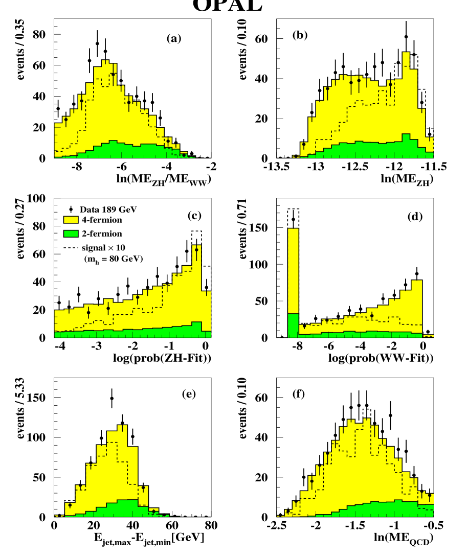
  Figure 1: Input variables of the four–jet channel likelihood selection for $m_{\mathrm{h}}$$=80$ $\mathrm{GeV}$. The OPAL data are indicated by dots with error bars (statistical errors), the 4-fermion background by lighter grey histograms, and the 2-fermion background by darker grey histograms. All MC distributions are normalised to the integrated luminosity of the data. The estimated contribution from an 80 $\mathrm{GeV}$ SM Higgs boson, scaled up by a factor of 10, is shown with a dashed line in each case.

  

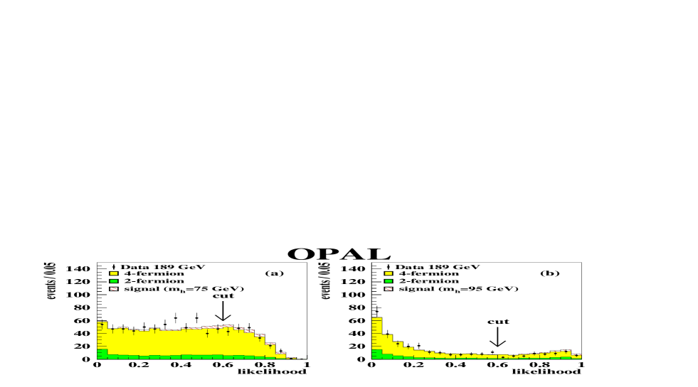
  Figure 2: Likelihood distribution of the four–jet channel for test masses of (a) $75$ $\mathrm{GeV}$ and (b) $95$ $\mathrm{GeV}$. The OPAL data are indicated by dots with error bars (statistical errors), the 4-fermion background by lighter grey histograms, and the 2-fermion background by darker grey histograms. The contributions expected from a (a) 75 $\mathrm{GeV}$ and (b) 95 $\mathrm{GeV}$ $\mathrm{h}^{0}$ boson assuming SM cross–section and branching ratios are shown as hatched histograms. All MC distributions are normalised to the integrated luminosity of the data. All events with a likelihood larger than 0.6 are accepted.

  equal to the mass of the W boson. Only the jet association that gives the highest fit probability is considered.

• The difference between the largest and the smallest jet energies in the event.

• The logarithm of an event weight, ME_QCD, formed [33] from the tree level matrix element for the process ${\mathrm{e}}^{+}{\mathrm{e}}^{-}$$\rightarrow$$\mathrm{q}\bar{\mathrm{q}}$$\mathrm{q}\bar{\mathrm{q}}$, $\mathrm{q}\bar{\mathrm{q}}$$\mathrm{g}\mathrm{g}$ [34], to reduce QCD background.

In Figure 1 the distributions of the likelihood input variables are shown for the difficult case in which $m_{\mathrm{h}}$$\approx$ $m_{\mathrm{W}}$.

The distributions of the final likelihood ${\cal L}^{\mathrm{h}Z}$ are shown in Figure 2 for test masses of $75$ and $95$ $\mathrm{GeV}$. Candidates for signal production are required to have ${\cal L}^{\mathrm{h}Z}>0.6$ for all test masses. In Table 3 the numbers of observed and expected events, together with the detection efficiencies for a Higgs signal with a mass of 80 $\mathrm{GeV}$, are given. Figure 3 compares the number of candidate events obtained after the likelihood selections for the different test masses with the expected background evaluated from Monte Carlo simulations. In the region of 75 $\mathrm{GeV}$, the number of expected background events rises to more than 200. This is due to the presence of $\mathrm{W}^{+}\mathrm{W}^{-}$ events, where the mass of one of the W bosons is constrained to the mass of the $\mathrm{Z}^{0}$, which reduces the other dijet mass by a few

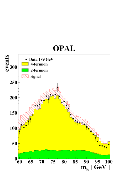
Figure 3: Number of events that pass the four–jet channel selection at each test mass. The number of candidates found in the data is indicated by dots with error bars (statistical errors), and the darker and lighter grey histograms correspond to the number of events expected from 2-fermion and 4-fermion backgrounds, respectively. The expected contribution from a Higgs boson with a mass equal to the test mass, assuming SM cross–sections and branching ratios, is shown by the hatched histogram. All MC distributions are normalised to the integrated luminosity of the data. Each bin corresponds to a different analysis of the same data, leading to a strong correlation between neighbouring bins.

$\mathrm{GeV}$ compared to the nominal value. The candidate masses are calculated from the momenta resulting from a 5C fit requiring energy and momentum conservation and forcing one of the dijet masses to $m_{\mathrm{Z}}$. Figure 4 shows the efficiency as a function of the Higgs mass for decays to b–quark, c-quark and gluon pairs separately as well as for a mixed sample according to SM branching ratios. For $m_{\mathrm{h}}$ between $80$ and $95$ $\mathrm{GeV}$ the efficiency reaches about $40$ to $45\%$ for quarks and $35$% for gluons. For small values of $m_{\mathrm{h}}$ it drops to $25\%$ due to the relatively large amount of initial state radiation that accompanies Higgs–strahlung when $m_{\mathrm{h}}$ is considerably lower than the kinematic limit, $i.e.$  $\sqrt{s}$$-$$m_{\mathrm{Z}}$. For the limit calculation, the efficiencies have been fitted to a polynomial function of $m_{\mathrm{h}}$ for each flavour separately, and at each mass point the lowest fitted polynomial is used. The signal selection efficiencies are affected by the uncertainties given below, expressed in relative percentages and shown as an example for a Higgs mass of $75$ $\mathrm{GeV}$. The systematic errors have been evaluated as follows: for each variable, the distributions obtained from the background Monte Carlo samples have been compared to those in the data. Then all Monte Carlo events (including the signal samples) have been reweighted so that the mean values of data and background distributions become the same and so that the sum of all

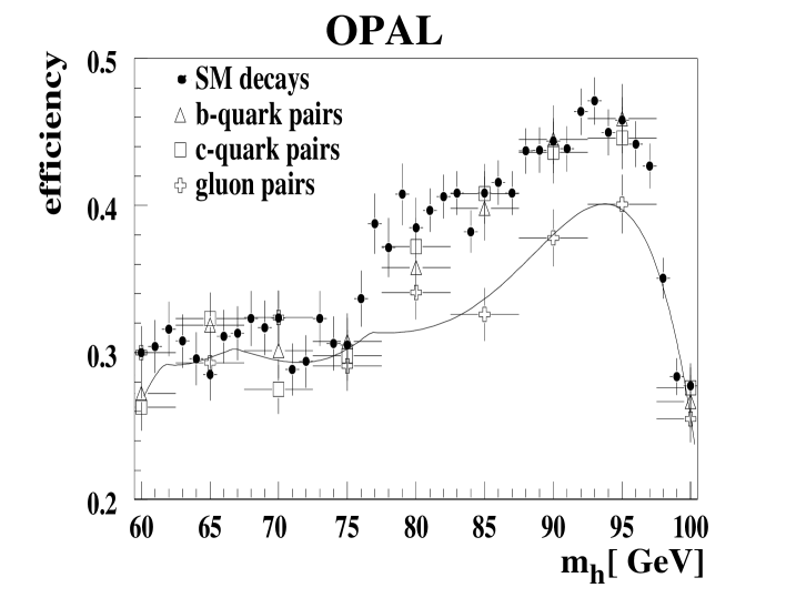
Figure 4: Efficiency of the four–jet channel selection as a function of $m_{\mathrm{h}}$  determined from different Monte Carlo samples. The dots represent the efficiency obtained from samples with SM branching ratios which also define the reference histograms at each test mass. The triangles, squares and crosses correspond to independent samples where the Higgs boson decays exclusively to b–quark, c–quark or gluon pairs, respectively. For the limit calculation, efficiencies have been fitted to a polynomial function of $m_{\mathrm{h}}$ for each flavour separately, and at each mass point the lowest fitted polynomial is used (black line).

weights is equal to $1$. The relative deviations in the number of events which pass the selection obtained by reweighting according to the different variables have been added in quadrature and amount to 5.5%. The same procedure has been applied to the kinematic likelihood variables, yielding an uncertainty of 2.0%. The uncertainty on the error parameterisation of the jet momenta used in the kinematic fits has been evaluated by varying the energy and angular resolutions by $\pm$10% , the energy scale by $\pm$ 1% and the centre–of–mass energy by $\pm$0.3 $\mathrm{GeV}$, each time repeating all kinematic fits. This leads to an uncertainty of 6.4%. Since the steps in the test mass are chosen to be smaller than the expected mass resolution, the deviation in efficiency due to the interpolation between test masses amounts only to 0.7%. The total systematic uncertainty on the signal selection efficiency has been calculated by adding the above sources in quadrature yielding 8.7%. All of these error contributions have been evaluated for masses of $60$ and $90$ GeV as well, leading to total systematic uncertainties of 9.8% and 7.1%, respectively. The Monte Carlo statistical error is about 2%.

The following uncertainties on the two major background sources are taken into account (the first number corresponds to the 4-fermion, the second number to the $\mathrm{q}\bar{\mathrm{q}}$($\gamma$) background, both for a test mass of $75$ $\mathrm{GeV}$): the uncertainty from modelling of the preselection cuts is evaluated as described above and amounts to 5.2%/4.5%. For the  likelihood  variables  this procedure  leads  to an  uncertainty  of 1.2%/1.6%.  Varying the

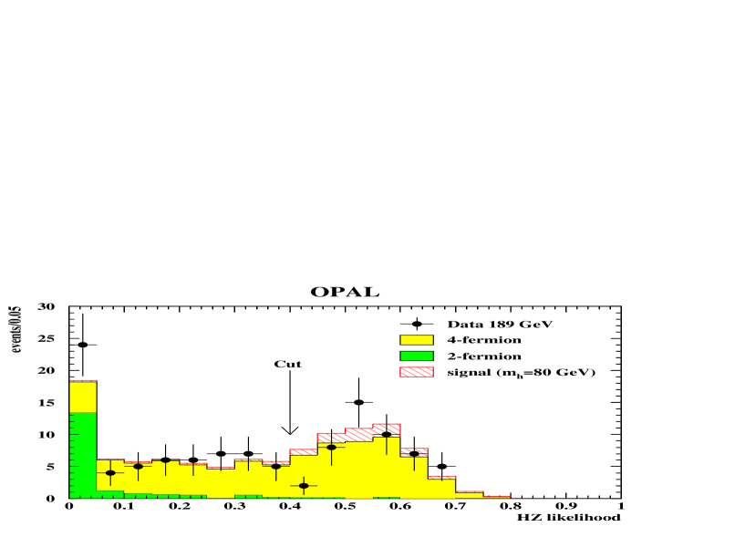
Figure 5: Likelihood output of the missing energy channel selection. The OPAL data are indicated by dots with error bars (statistical errors), the 4-fermion background by the lighter grey histogram, and the 2-fermion background by the darker grey histogram. The estimated contribution from an 80 $\mathrm{GeV}$ Higgs with SM cross–section and branching ratios is shown as a hatched histogram. All MC distributions are normalised to the integrated luminosity of the data.

error parameterisations, energy scale and centre–of–mass energy for the kinematic fits yields an uncertainty of 3.0%/8.1%. Different Monte Carlo generators have been used to evaluate the background from 4-fermion events (EXCALIBUR instead of grc4f) and QCD events (HERWIG instead of PYTHIA) resulting in an uncertainty of 2.2%/12.3%. The total systematic uncertainty on the residual background estimate amounts to 10.3%. For test masses of $60$ and $90$ $\mathrm{GeV}$ the total systematic uncertainties amount to 12.4% and 8.3%, respectively. The largest Monte Carlo statistical error is 1.3%.

4.2 The missing–energy channel

This analysis is nearly identical to a previous one, of which a detailed description can be found in [29], with the exception that the b–tagging is not applied. The preselection is unchanged. The same kinematic variables used previously, as well as the acollinearity angle and the total missing transverse momentum, are combined using a likelihood technique. In Figure 5, the resulting signal likelihood distribution is shown for the data, SM backgrounds, and an example signal at $m_{\mathrm{h}}=80$ GeV. The signal likelihood is required to be larger than 0.4 for an event to be selected as a Higgs candidate.

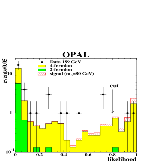
Figure 6: Likelihood output of the tau channel selection for events satisfying the $\mathrm{h}^{0}$$\mathrm{Z}^{0}$$\rightarrow$$\mathrm{q}\bar{\mathrm{q}}$$\tau^{+}\tau^{-}$ kinematic hypothesis. OPAL data are indicated by dots with error bars (statistical errors), 4-fermion background by the lighter grey histogram, and 2-fermion background by the darker grey histogram. The contribution expected from an 80 GeV Higgs with SM cross–section and branching ratios is shown as a hatched histogram. All MC distributions are normalised to the integrated luminosity of the data.

The reconstructed mass in selected events is evaluated using a kinematic fit constraining the recoil mass to the $\mathrm{Z}^{0}$ mass. The numbers of observed and expected events are given in Table 3, together with the selection efficiencies for an 80 GeV Higgs. The selection efficiency has been estimated from Monte Carlo samples generated separately for b–quark, c–quark and gluon pairs. The efficiency is the lowest and the width of the reconstructed Higgs mass is the largest for c–quark pairs and therefore they are used in the limit calculation. For an 80 GeV Higgs, the efficiency is (51.0$\pm$1.7(stat.)$\pm$1.3(syst.))%. The efficiency has been optimised for Higgs masses between 70 and 90 $\mathrm{GeV}$. Outside this range, the efficiency decreases and reaches about 20% for masses of 60 and 100 $\mathrm{GeV}$. For b–quarks, the efficiency is about 5% (relative) higher throughout the whole mass range. A total of 47 data events pass the selection, while 44.5$\pm$1.4(stat.)$\pm$3.0(syst.) events are expected from SM background processes. The systematic error has been evaluated as in [29], but b–tagging related errors have been omitted.

4.3 The tau channel

The preselection, the tau lepton identification using an artificial neural network, and the two–tau likelihood, $\mathcal{L}_{\tau\tau}$, used in this channel are unchanged with respect to the analysis described in reference  [30]. Since b–tagging information is not used, for the final selection the likelihood $\mathcal{L}(\mbox{$\mathrm{q}\bar{\mathrm{q}}$}\mbox{$\tau^{+}\tau^{-}$})$  [30] is used and required to exceed 0.8. Additionally, the $\chi^{2}$–probability of a kinematic fit, which constrains the invariant mass of the two $\tau$’s to $m_{\mathrm{Z}}$, should be larger than $10^{-5}$, since this analysis is designed to be sensitive to hadronic Higgs boson decays and to $\mathrm{Z}^{0}$$\rightarrow$$\tau^{+}\tau^{-}$. In Figure 6 the resulting likelihood distributions are shown for the data, SM backgrounds, and an example signal at $m_{\mathrm{h}}=80$ GeV. The numbers of observed and expected events are given in Table 3, together with the selection efficiencies for an 80 GeV Higgs. The signal detection efficiency has been evaluated for b–quark, c–quark and gluon pairs separately and at each mass the lowest value is taken for the limit calculation. For an 80 $\mathrm{GeV}$ Higgs boson it amounts to (28.7 $\pm$ 1.5(stat.)$\pm$ 2.7(syst.))% after all the selection requirements. For lower and higher Higgs masses, the efficiency drops to about 20% at $m_{\mathrm{h}}$$=50$ $\mathrm{GeV}$ and $m_{\mathrm{h}}$$=100$ $\mathrm{GeV}$. Two events survive the likelihood cut, which can be compared to the expected background of $3.4\pm 0.5(\mathrm{stat}.)\pm 0.7(\mathrm{syst}.)$. The systematic errors quoted above for signal and background are evaluated with the method described in [29], with the contributions from fragmentation and decay multiplicity of b–quarks omitted.

4.4 The electron and muon channels

The preselection cuts and kinematic likelihood $\cal K$ are identical to the analysis described in  [29]. Because the present analysis is intended to be independent of the flavour of the Higgs decay products, no b–tagging is applied and $\cal K$ is used as the final selection variable, which should exceed 0.3 for the electron and 0.65 for the muon channel. Figure 7 shows the distribution of $\cal K$ for the electron (a) and the muon (b) channel.

The signal selection efficiency has been evaluated and fitted for each flavour separately. For the limit calculation, the lowest of these efficiencies at each mass point has been used. For an 80 GeV Higgs boson it amounts to (55.4$\pm$1.6(stat.)$\pm$0.6(syst.))% for the electron channel, and (59.3$\pm$1.5(stat.)$\pm$0.7(syst.))% for the muon channel. In the electron channel, the efficiency lies between 50% and 55% for all Higgs masses between 60 and 95 $\mathrm{GeV}$, and drops to 27% for a Higgs mass of 100 $\mathrm{GeV}$. In the muon channel, the efficiency is between 55% and 70% for all Higgs masses under consideration.

The numbers of observed and expected events are given in Table 3, together with the detection efficiency for an 80 GeV SM Higgs boson. The selection retains 7 events in the electron channel and 3 in the muon channel. The total background expectation is 4.7$\pm$0.2(stat.)$\pm$1.4(syst.) events in the electron channel and 4.7$\pm$0.1(stat.)$\pm$0.9(syst.) events in the muon channel.

The systematic errors quoted above for signal and background are evaluated with the method described in [29]. The largest contribution to the systematic error on the background expectation is due to differences between various Monte Carlo generators.

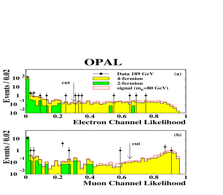
Figure 7: (a) The electron and (b) the muon channel likelihood distributions. The OPAL data are indicated by dots with error bars (statistical), the 4-fermion background by lighter grey histograms, and the 2-fermion background by darker grey histograms. The contributions expected from an 80 $\mathrm{GeV}$ Higgs with SM cross–section and branching ratios are shown as hatched histograms. All MC distributions are normalised to the integrated luminosity of the data.

4.5 Summary of the flavour independent searches for
${\mathrm{e}}^{+}{\mathrm{e}}^{-}$$\rightarrow$$\mathrm{h}^{0}$$\mathrm{Z}^{0}$

The total numbers of candidates accepted after the preselection and the flavour independent likelihood cut, compared to the expected SM backgrounds as well as the detection efficiencies for a hadronically decaying Higgs boson with a mass of 80 $\mathrm{GeV}$, are summarised in Table 3, together with the expected number of signal events in the 2HDM(II) for the case of $\alpha$ = 0, $\tan\!\beta$ = 1.0 and $m_{\mathrm{h}}$ = 80 GeV. The total number of observed candidates for an 80 $\mathrm{GeV}$ Higgs boson is 246, while the background expectation amounts to $231.3\pm 4.4({\mathrm{s}tat.})\pm 18.0({\mathrm{s}yst.})$.

Cut	Data	Total bkg.	qq̄($\gamma$)	4–fermion	Efficiency [%]	Signal
Four–jet Channel    ${\cal L}$ = 174.1 pb-1
Preselection	1568	1521	379	1142	87.4	31.8
(1)	696	649	117	532	65.3	23.8
(2)	648	600	116	484	64.1	23.3
Likelihood	187	174	28	146	35.4	12.9
Missing–energy Channel    ${\cal L}$ = 171.8 pb-1
Preselection	111	101	18	83	63.4	6.5
Likelihood	47	44.5	0.6	43.9	51.0	5.3
Tau Channel    ${\cal L}$ = 168.7 pb-1
Preselection	185	156	55	101	49.1	0.8
Likelihood	2	3.4	0.1	3.3	28.7	0.5
Electron Channel ${\cal L}$ = 172.1 pb-1
Preselection	152	153	84	69	77.8	1.4
Likelihood	7	4.7	0.1	4.5	55.4	1.0
Muon Channel ${\cal L}$ = 169.4 pb-1
Preselection	22	22	14	8	78.8	1.3
Likelihood	3	4.7	0.0	4.7	59.3	1.0

Table 3: The $\mathrm{h}^{0}$$\mathrm{Z}^{0}$ channels for the flavour independent analysis: the numbers of events selected in the data at $\sqrt{s}$ = 189 GeV, expected background from SM processes normalised to the data luminosity (given for each channel), the minimal detection efficiencies for a Higgs boson with a mass of 80 $\mathrm{GeV}$ decaying to quark or gluon pairs and the expected number of signal events within the 2HDM(II) for the case of $\alpha$ = 0, $\tan\!\beta$ = 1.0 and $m_{\mathrm{h}}$ = 80 GeV, after the preselection and the flavour independent likelihood cut. In the case of the four–jet channel, after preselection, the numbers of events are given for the selection with an 80 GeV test mass.

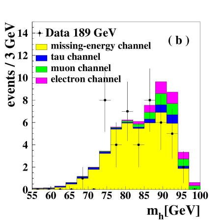
Figure 8: Mass distributions for selected data events and SM background expectation (a) for all channels and (b) for all channels except the four–jet channel. OPAL data are indicated by dots with error bars (statistical) while the background contributions from the various channels are shown in different shades of grey. For the four–jet channel the 90 $\mathrm{GeV}$ analysis is shown.

The mass distributions for candidates found in the data as well as for the background expected from the SM for all flavour independent channels are shown in Figure 8(a). The same mass distributions without the four–jet channel contribution are shown in Figure 8(b).

5 Flavour independent search for ${\mathrm{e}}^{+}{\mathrm{e}}^{-}$$\rightarrow$$\mathrm{h}^{0}$$\mathrm{A}^{0}$

We have searched for the process ${\mathrm{e}}^{+}{\mathrm{e}}^{-}$$\rightarrow$$\mathrm{h}^{0}$$\mathrm{A}^{0}$ in the final states $\mathrm{q}\bar{\mathrm{q}}$$\mathrm{q}\bar{\mathrm{q}}$, $\mathrm{g}\mathrm{g}$$\mathrm{q}\bar{\mathrm{q}}$ and $\mathrm{g}\mathrm{g}$$\mathrm{g}\mathrm{g}$. The signal is characterised by events with four well-separated jets with characteristic invariant masses of the dijet pairs originating from the $\mathrm{h}^{0}$ and the $\mathrm{A}^{0}$. The dominant background is from the process ${\mathrm{e}}^{+}{\mathrm{e}}^{-}$$\rightarrow$$\mathrm{W}^{+}$$\mathrm{W}^{-}$$\rightarrow$$\mathrm{q}\bar{\mathrm{q}}$$\mathrm{q}\bar{\mathrm{q}}$. The second-largest contribution comes from ${\mathrm{e}}^{+}{\mathrm{e}}^{-}$$\rightarrow$$\mathrm{Z}^{0}$$/\gamma$$\rightarrow$$\mathrm{q}\bar{\mathrm{q}}$ with multiple hard gluon radiation producing a four–jet final state.

This search is designed to be sensitive over a large portion of the ($m_{\mathrm{h}}$, $m_{\mathrm{A}}$) plane, and the kinematic signatures of signal events depend strongly on $m_{\mathrm{h}}$ and $m_{\mathrm{A}}$. For this reason, a loose selection is performed first, retaining four-jet hadronic events with partial rejection of $\mathrm{W}^{+}$$\mathrm{W}^{-}$ and Z⁰Z⁰ events. The main discrimination, however, is achieved by constraining candidate events to the signal mass hypothesis ($m_{\mathrm{h}}$ and $m_{\mathrm{A}}$), and using the logarithm of the resulting $\chi^{2}$ as the discriminant variable in the limit calculation instead of the reconstructed dijet masses. This choice of variable also incorporates naturally the measurement uncertainties on the reconstructed masses and simplifies the interpolation of its shape as a function of $m_{\mathrm{h}}$ and $m_{\mathrm{A}}$.

5.1 Selection

Candidate events must first satisfy the requirements of a preselection and then a loose selection based on a likelihood variable which is built out of reference distributions of reconstructed quantities for events passing the preselection. The following criteria are applied ((1)–(4) preselection, (5) selection):

• Each candidate event is required to be classified as a hadronic final state [35] with an effective centre-of-mass energy $\sqrt{s^{\prime}}$ exceeding 150 GeV. The jet resolution parameter in the Durham scheme [13] $y_{34}$ is required to be larger than 0.003 in order to select events with four distinct jets.

• Each jet must have at least three tracks.

• The $\chi^{2}$ probability of a 4C fit, requiring energy and momentum conservation, must be greater than $10^{-5}$, to ensure that the mass reconstructions used to isolate the signal do not suffer from poor measurement or energy loss from initial state radiation.

• A 6C kinematic fit is performed requiring energy and momentum conservation and also that the invariant masses of the dijet pairs are equal to $m_{\mathrm{W}}$. The 6C fit $\chi^{2}$ probability of each of the three possible jet combinations is required to be less than 0.01, to reduce the background from hadronic $\mathrm{W}^{+}$$\mathrm{W}^{-}$ decays.

• A likelihood composed of five variables is computed. These variables are the jet resolution parameter $y_{34}$, the event-shape variable $C$ obtained from the eigenvalues of the sphericity tensor [36], the smallest angle between any two jets in the event, the logarithm of the QCD matrix element ME_QCD [34], and the largest $\chi^{2}$ probability of three 5C kinematic fits constraining energy and momentum and requiring the equality of the masses of the two dijet systems (three possible pairings). The QCD matrix element used is the maximum of the matrix elements considering all possible assignments of observed jets to partons in the ${\mathrm{e}}^{+}{\mathrm{e}}^{-}$$\rightarrow$$\mathrm{q}\bar{\mathrm{q}}$$\mathrm{q}\bar{\mathrm{q}}$ and ${\mathrm{e}}^{+}{\mathrm{e}}^{-}$$\rightarrow$$\mathrm{q}\bar{\mathrm{q}}$$\mathrm{g}\mathrm{g}$ processes. The first four variables are designed to separate the signal from the $\mathrm{q}\bar{\mathrm{q}}$ background. The last variable provides rejection of the diboson backgrounds from $\mathrm{W}^{+}$$\mathrm{W}^{-}$ and Z⁰Z⁰ events surviving the 6C fit probability requirement (4). Although its use reduces the efficiency for signals with $m_{\mathrm{h}}$ = $m_{\mathrm{A}}$, the sensitivity to signals with $m_{\mathrm{h}}$ $\neq$ $m_{\mathrm{A}}$ is enhanced. The signal samples used to form reference distributions for the likelihood are a mixture of samples in the kinematically accessible region of the ($m_{\mathrm{h}}$, $m_{\mathrm{A}}$) plane with $m_{\mathrm{h}}$, $m_{\mathrm{A}}$ $>$ 30 GeV. The distribution of this likelihood variable for the data, SM backgrounds, and a representative signal with $m_{\mathrm{h}}$ = 30 GeV and $m_{\mathrm{A}}$ = 60 GeV is shown in Figure 9. The likelihood variable is required to exceed 0.1 for selected events.

In Table 4 the numbers of events passing the requirements after each step, (1) to (5), are given, together with the expected SM backgrounds from 4-fermion and 2-fermion processes. The lowest estimated efficiencies, for $m_{\mathrm{h}}$ = 30 GeV and $m_{\mathrm{A}}$ = 60 GeV, corresponding to the $\mathrm{b}\bar{\mathrm{b}}$$\mathrm{b}\bar{\mathrm{b}}$ final state, and the number of expected signal events in the 2HDM(II) for the case of $\alpha$ = 0, $\tan\!\beta$ = 1.0, $m_{\mathrm{h}}$ = 30 GeV and $m_{\mathrm{A}}$ = 60 GeV, are shown in the last two columns.

Cut	Data	Total bkg.	$\mathrm{q}\bar{\mathrm{q}}$($\gamma$)	4-fermion	Efficiency [%]	Signal
(1)	1953	1885.0	537.8	1347.2	51.2	14.9
(2)	1593	1532.0	410.1	1121.9	47.9	13.9
(3)	1497	1446.3	376.1	1070.2	44.3	12.9
(4)	904	895.0	329.2	565.8	40.0	11.6
(5)	573	553.2	238.5	314.7	38.5	11.2

Table 4: The $\mathrm{h}^{0}$$\mathrm{A}^{0}$ channel for the flavour independent analysis: the numbers of events selected in the data at $\sqrt{s}$ = 189 GeV, expected background from SM processes normalised to the data luminosity of 172.1 pb^-1, the minimal detection efficiencies for $m_{\mathrm{h}}$ = 30 GeV, $m_{\mathrm{A}}$ = 60 GeV and the expected number of signal events within the 2HDM(II) for the case of $\alpha$ = 0, $\tan\!\beta$ = 1.0, $m_{\mathrm{h}}$ = 30 GeV and $m_{\mathrm{A}}$ = 60 GeV after each step of the selection.

The selection efficiency is estimated with the Monte Carlo simulation at a discrete set of reference points in the ($m_{\mathrm{h}}$, $m_{\mathrm{A}}$) plane. The efficiency function is interpolated by considering the three closest reference points. A plane in the ($m_{\mathrm{h}}$, $m_{\mathrm{A}}$, efficiency) space is formed containing those three points, which allows the efficiency for an arbitrary intermediate ($m_{\mathrm{h}}$, $m_{\mathrm{A}}$) signal hypothesis to be computed. The interpolated efficiency function is shown in Figure 10 for the final-state flavour assignment with the lowest efficiency. The efficiency is low near $m_{\mathrm{h}}$ = $m_{\mathrm{A}}$ = $m_{\mathrm{W}}$ because of the difficulty in distinguishing hadronic $\mathrm{h}^{0}$$\mathrm{A}^{0}$ decays from hadronic $\mathrm{W}^{+}$$\mathrm{W}^{-}$ decays. The veto of $\mathrm{W}^{+}$$\mathrm{W}^{-}$  events reduces the efficiency in the entire ($m_{\mathrm{h}}$, $m_{\mathrm{A}}$) plane because incorrect jet assignments in $\mathrm{h}^{0}$$\mathrm{A}^{0}$ events can produce interpretations consistent with the $\mathrm{W}^{+}$$\mathrm{W}^{-}$ hypothesis. Conversely, the $\mathrm{W}^{+}$$\mathrm{W}^{-}$ veto reduces the background of incorrectly-paired $\mathrm{W}^{+}$$\mathrm{W}^{-}$ events everywhere in the ($m_{\mathrm{h}}$, $m_{\mathrm{A}}$) plane. The efficiency for low $m_{\mathrm{h}}$ and $m_{\mathrm{A}}$ is reduced because of the requirement that the event should have four distinct jets, which helps to reject the $\mathrm{q}\bar{\mathrm{q}}$ background.

After the selection, 573 candidates remain in the data, as compared with the SM expectation of 553.2$\pm$38.2 events.

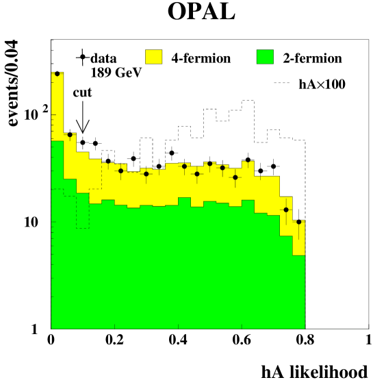
Figure 9: Likelihood distribution for the flavour independent ${\mathrm{e}}^{+}{\mathrm{e}}^{-}$$\rightarrow$$\mathrm{h}^{0}$$\mathrm{A}^{0}$ channel. The OPAL data are indicated by dots with error bars (statistical error), the 4-fermion background by the lighter grey histogram, the 2-fermion background by the darker grey histogram and a representative signal for $m_{\mathrm{h}}$ = 30 GeV, $m_{\mathrm{A}}$ = 60 GeV by the dashed histogram. All Monte Carlo distributions are normalised to the data luminosity and the signal is scaled by a factor of 100.

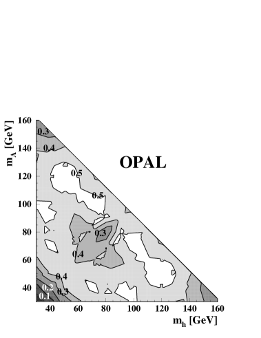
Figure 10: Lowest efficiency contours for the flavour independent search for hadronic $\mathrm{h}^{0}$$\mathrm{A}^{0}$ events. The efficiency is taken to be zero for $m_{\mathrm{h}}$$\mathrm{+}$$m_{\mathrm{A}}$$>189$ GeV.

5.2 Discriminant variable

The invariant masses of jet pairs may be used to separate possible $\mathrm{h}^{0}$$\mathrm{A}^{0}$ signals from the $\mathrm{W}^{+}$$\mathrm{W}^{-}$ and $\mathrm{q}\bar{\mathrm{q}}$$\mathrm{g}\mathrm{g}$ backgrounds. There are six possible assignments of pairs of jets to $\mathrm{h}^{0}$ and $\mathrm{A}^{0}$ bosons, and there is no constraint from a known mass such as that of the $\mathrm{Z}^{0}$ used in the ${\mathrm{e}}^{+}{\mathrm{e}}^{-}$$\rightarrow$$\mathrm{h}^{0}$$\mathrm{Z}^{0}$ channels. All six possible interpretations of each selected event are tested for consistency with a possible signal. When computing the confidence level for excluding a model hypothesis, only a single interpretation of each candidate in the data and Monte Carlo samples may be used. The choice of jet pairing depends on the $m_{\mathrm{h}}$ and $m_{\mathrm{A}}$ of the hypothesised signal.

For each event passing the selection, a 4C kinematic fit constraining energy and momentum conservation is performed. For each of the assignments of jet pairs to bosons, the reconstructed $m_{\mathrm{h}}$ and $m_{\mathrm{A}}$ are computed, along with their covariance matrices. For each hypothetical $m_{\mathrm{h}}$ and $m_{\mathrm{A}}$ considered in the limit computation, each event is assigned the jet pairing with the smallest $\chi^{2}$ value resulting from the difference of the measured and hypothesised $m_{\mathrm{h}}$ and $m_{\mathrm{A}}$, and the error matrix of the measurement. The logarithm of the smallest $\chi^{2}$ is then used as the discriminating variable when computing limits because the signal to background ratio depends strongly on the value of $\log\chi^{2}$. Figure 11 shows the distribution of $\log\chi^{2}$ for selected data events, the SM expectation, and the signal for four mass hypotheses. The signal shown corresponds to the ${\mathrm{e}}^{+}{\mathrm{e}}^{-}$$\rightarrow$$\mathrm{h}^{0}$$\mathrm{A}^{0}$$\rightarrow$$\mathrm{g}\mathrm{g}$$\mathrm{g}\mathrm{g}$ process because of its poorer mass resolution compared with that obtained for final states with quarks.

For $m_{\mathrm{h}}$ = $m_{\mathrm{A}}$ = $m_{\mathrm{W}}$, the separation between the signal and the background is poor, while for lower values of $m_{\mathrm{h}}$ or $m_{\mathrm{A}}$ the separation is better. The resolution on the reconstructed sum of the dijet masses is approximately 2.4 GeV, while for the difference it is approximately 6.2 GeV. The best sensitivity to the signal is in regions of ($m_{\mathrm{h}}$, $m_{\mathrm{A}}$) with dijet mass sums different from 2$m_{\mathrm{W}}$. The test mass spacing is determined by the model scan grid used when computing the limits – no discretization is introduced within the analysis. The scan grid used to compute limits has a finer spacing than the mass resolutions on the candidates. All candidates are considered at all test mass hypotheses – they simply appear at different locations in the $\log\chi^{2}$ histogram. The distribution of the $\chi^{2}$ variable for the signal and backgrounds changes slowly with the test mass hypothesis and is interpolated between Monte Carlo samples generated at different test masses.

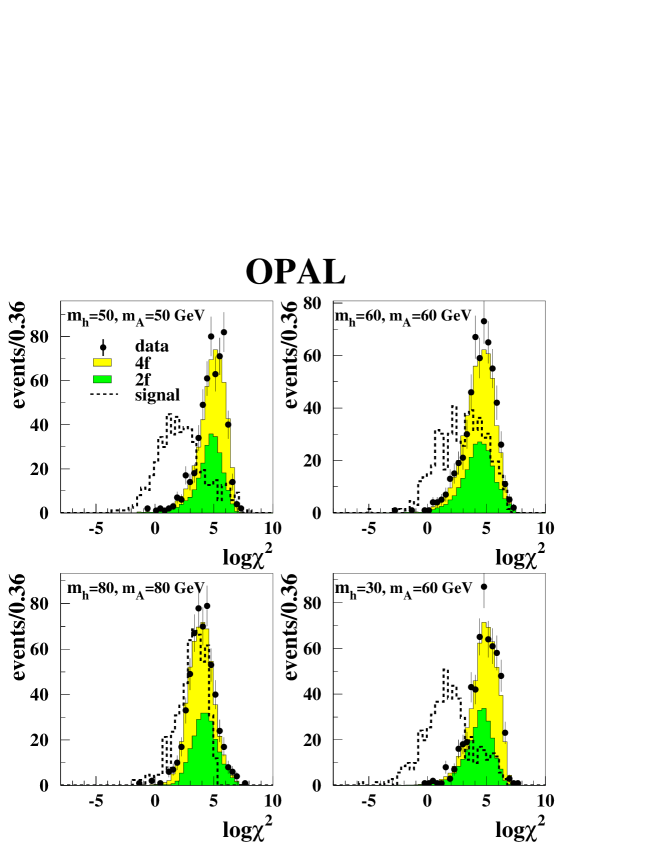
Figure 11: Distribution of $\log\chi^{2}$ of the mass constraint for the flavour independent ${\mathrm{e}}^{+}{\mathrm{e}}^{-}$$\rightarrow$$\mathrm{h}^{0}$$\mathrm{A}^{0}$ channel for four hypotheses of ($m_{\mathrm{h}}$, $m_{\mathrm{A}}$). The OPAL data are indicated by dots with error bars (statistical errors), the 4-fermion backgrounds by lighter grey histograms and the 2-fermion background by darker grey histograms. The ${\mathrm{e}}^{+}{\mathrm{e}}^{-}$$\rightarrow$$\mathrm{h}^{0}$$\mathrm{A}^{0}$$\rightarrow$$\mathrm{g}\mathrm{g}$$\mathrm{g}\mathrm{g}$ signals are shown with arbitrary normalizations by dashed histograms.

Systematic uncertainties have been considered on the signal and background normalisation and shapes. The ${\mathrm{e}}^{+}{\mathrm{e}}^{-}$$\rightarrow$$\mathrm{W}^{+}$$\mathrm{W}^{-}$ cross-section is taken to be uncertain at the level of 2% from a comparison of the predictions of the GENTLE and EXCALIBUR calculations. The selection efficiency for ${\mathrm{e}}^{+}{\mathrm{e}}^{-}$$\rightarrow$$\mathrm{W}^{+}$$\mathrm{W}^{-}$ events is uncertain at the level of approximately 1%, from sensitivity to fragmentation modelling in hadronic W decays and from comparisons of the selection variables in data and Monte Carlo [37]. The background from $\mathrm{Z}^{0}$/$\gamma\rightarrow$$\mathrm{q}\bar{\mathrm{q}}$$(\gamma)$ has an 11% uncertainty [38], which includes the uncertainty on the selection efficiency and on the four–jet rate in $\mathrm{q}\bar{\mathrm{q}}$ events, which is the dominant contribution. The 4-fermion background from two neutral vector gauge bosons has been estimated using the grc4f Monte Carlo generator for the central value, and its uncertainty has been estimated by comparing the results obtained with the grc4f and EXCALIBUR generators. Scaling these uncertainties by their fractional contributions to the background of this selection and adding the results in quadrature yields an uncertainty on the background normalisation of 6.9%. Monte Carlo statistics accounts for only a 1% relative error on the background.

The uncertainty on the signal efficiencies is dominated by the flavour dependence, with the highest selection efficiency for the $\mathrm{g}\mathrm{g}$$\mathrm{g}\mathrm{g}$ final state. The $\mathrm{b}\bar{\mathrm{b}}$$\mathrm{b}\bar{\mathrm{b}}$ and $\mathrm{c}\bar{\mathrm{c}}$$\mathrm{c}\bar{\mathrm{c}}$ final states have very similar selection efficiencies. The lowest signal efficiency at each mass hypothesis is used in the limit calculations.

A more significant effect on the modelling of the signal is the uncertainty in the reconstructed mass resolution, as this affects the shape of the $\log\chi^{2}$ distribution of the signal and hence the limits. Similar performances are achieved in Monte Carlo simulations of the $\mathrm{b}\bar{\mathrm{b}}$$\mathrm{b}\bar{\mathrm{b}}$ and $\mathrm{c}\bar{\mathrm{c}}$$\mathrm{c}\bar{\mathrm{c}}$ final states, but the $\mathrm{g}\mathrm{g}$$\mathrm{g}\mathrm{g}$ final state has on average a positive shift of one unit of $\log\chi^{2}$ relative to the four-quark final states because the resolution is poorer for reconstructing masses from gluon jets. The conservative approach of using the $\log\chi^{2}$ distribution of $\mathrm{g}\mathrm{g}$$\mathrm{g}\mathrm{g}$ signal final states has been adopted when computing the limits.

6 Model–independent interpretation

The results of all the individual search channels at the studied centre–of–mass energies are combined statistically to provide 95% confidence level (CL) limits in a model–independent interpretation in which no assumption is made on the structure of the Higgs sector. The limits are extracted using the same method applied in previous OPAL publications  [32, 39].

Model–independent   limits  are  given  for  the   cross-section  of  the  generic  processes
${\mathrm{e}}^{+}{\mathrm{e}}^{-}$$\rightarrow$ S⁰$\mathrm{Z}^{0}$ and ${\mathrm{e}}^{+}{\mathrm{e}}^{-}$$\rightarrow$ S⁰P⁰, where S⁰ and P⁰ denote scalar and pseudo-scalar neutral bosons, respectively. The limits are conveniently expressed in terms of scale factors, $s^{2}$ and $c^{2}$  [29], which relate the cross-sections of these generic processes to SM cross-sections (c.f. Eqs. (9), (10)):

$$\sigma_{\mathrm{SZ}}=s^{2}~{}\sigma^{\mathrm{SM}}_{\mathrm{HZ}},$$ (12)

$$\sigma_{\mathrm{SP}}=c^{2}~{}\bar{\lambda}~{}\sigma^{\mathrm{SM}}_{\mathrm{HZ}}.$$ (13)

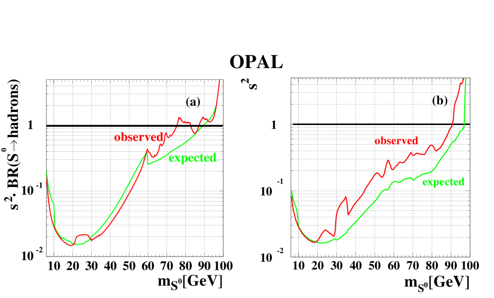
Figure 12: Observed and expected upper limits at 95% CL on (a) $s^{2}\cdot$BR($\mathrm{h}^{0}$$\rightarrow$ hadrons) using flavour independent channels, and (b) $s^{2}$ using all $\mathrm{S^{0}}$$\mathrm{Z}^{0}$ search channels with b–tagging and assuming SM Higgs branching ratios for the S⁰.

Figure 12 shows the 95% CL upper bound for $s^{2}$ as a function of the S⁰ mass, obtained from:

$$s^{2}=\frac{N_{95}^{\mathrm{SZ}}}{\sum~{}(\epsilon~{}{\cal L}~{}\sigma^{\mathrm{SM}}_{\mathrm{HZ}})},$$

where $N^{\mathrm{SZ}}_{95}$ is the 95% CL upper limit on the number of possible signal events in the data, $\epsilon$ is the signal detection efficiency, ${\cal L}$ is the integrated luminosity, and the sum runs over the different centre-of-mass energies of the data and the different channels. In Figure 12(a) only the flavour independent channels described in Section 4 and the channels analysed at the $\mathrm{Z}^{0}$ pole are used to extract a 95% CL upper limit on $s^{2}\cdot$BR(S⁰$\rightarrow$hadrons). In Figure 12(b) the SM Higgs branching ratios for the S⁰ are assumed and search channels with b–tagging are used. In the region $m_{\mathrm{S}}<30$ GeV the high energy data (LEP2) have little exclusion power while for $m_{\mathrm{S}}>50$ GeV the $\mathrm{Z}^{0}$ data (LEP1) contribute little to the determination of the experimental limit. The $s^{2}$ limit is calculated only for $m_{\mathrm{S}}$ $\geq 5$ GeV, since below this mass value the direct search rapidly loses sensitivity and the limit is extracted by a different method  [40], which makes use of the electroweak precision measurements of the $\mathrm{Z}^{0}$ width and provides an $s^{2}$ limit of about $0.5\times 10^{-2}$.

The limit on $m_{\mathrm{S}}$ for $s^{2}=$ 1 assuming SM branching ratios is 91 GeV in complete agreement with the result obtained by the SM search  [30] at $\sqrt{s}$$\approx$ 189 GeV. A limit of 75 GeV on $m_{\mathrm{S}}$ for $s^{2}=$ 1 is obtained when assuming a 100% hadronic branching ratio. This weaker limit is partly due to the presence of candidates around $m_{\mathrm{S}}$ $\approx$ 80 GeV as can be seen from the different behaviour of the observed and expected limit in Figure 12(a).

Iso-contours of 95% CL upper limits for $c^{2}$ in the S⁰ and P⁰ mass plane are shown for the processes S⁰P⁰$\rightarrow$$\mathrm{q}\bar{\mathrm{q}}$$\mathrm{q}\bar{\mathrm{q}}$, $\mathrm{g}\mathrm{g}$$\mathrm{q}\bar{\mathrm{q}}$ and $\mathrm{g}\mathrm{g}$$\mathrm{g}\mathrm{g}$ in Figure 13(a), and for ${\mathrm{e}}^{+}{\mathrm{e}}^{-}$$\rightarrow$ S⁰P⁰$\rightarrow$$\mathrm{b}\bar{\mathrm{b}}$$\mathrm{b}\bar{\mathrm{b}}$ and $\mathrm{b}\bar{\mathrm{b}}$$\tau^{+}\tau^{-}$ in Figures 13(b) and (c), respectively, assuming a 100% branching ratio into the specific final states. The contours are obtained from:

$$c^{2}=\frac{N_{95}^{\mathrm{SP}}}{\sum~{}(\epsilon~{}{\cal L}~{}\bar{\lambda}~{}\sigma^{\mathrm{SM}}_{HZ})},$$

with $N_{95}^{\mathrm{SP}}$ being the 95% CL upper limit for the number of signal events in the data. The results obtained in Figures 13(a) and (b) are symmetric with respect to interchanging of S⁰ and P⁰, while those obtained for $\tau^{+}\tau^{-}$$\mathrm{b}\bar{\mathrm{b}}$ are not. For this reason, the results for $\tau^{+}\tau^{-}$$\mathrm{b}\bar{\mathrm{b}}$ are presented with the mass of the particle decaying into $\tau^{+}\tau^{-}$ along the abscissa and that of the particle decaying into $\mathrm{b}\bar{\mathrm{b}}$ along the ordinate. The irregularities of the iso-$c^{2}$ contours are due to the presence of candidate events. Along the diagonal, for $c^{2}=1$, a lower bound is extracted using the b–tagging channels on the masses at $m_{\mathrm{S}}=m_{\mathrm{P}}\approx m_{\mathrm{\tau^{+}\tau^{-}}}\approx m_{\mathrm{b\bar{b}}}>78$ GeV at 95% CL. In the hypothesis of S⁰ P⁰ decaying to hadrons with a 100% branching ratio, a lower bound of $m_{\mathrm{S}}=m_{\mathrm{P}}>61$ GeV is obtained along the diagonal for $c^{2}$ = 1. Note the small region 30 $\leq m_{\mathrm{P}},~{}m_{\mathrm{S}}\leq$ 40 GeV in Figures 13(a) and (b) which is excluded by the flavour independent search but not when using only $\mathrm{b}\bar{\mathrm{b}}$$\mathrm{b}\bar{\mathrm{b}}$ channels.

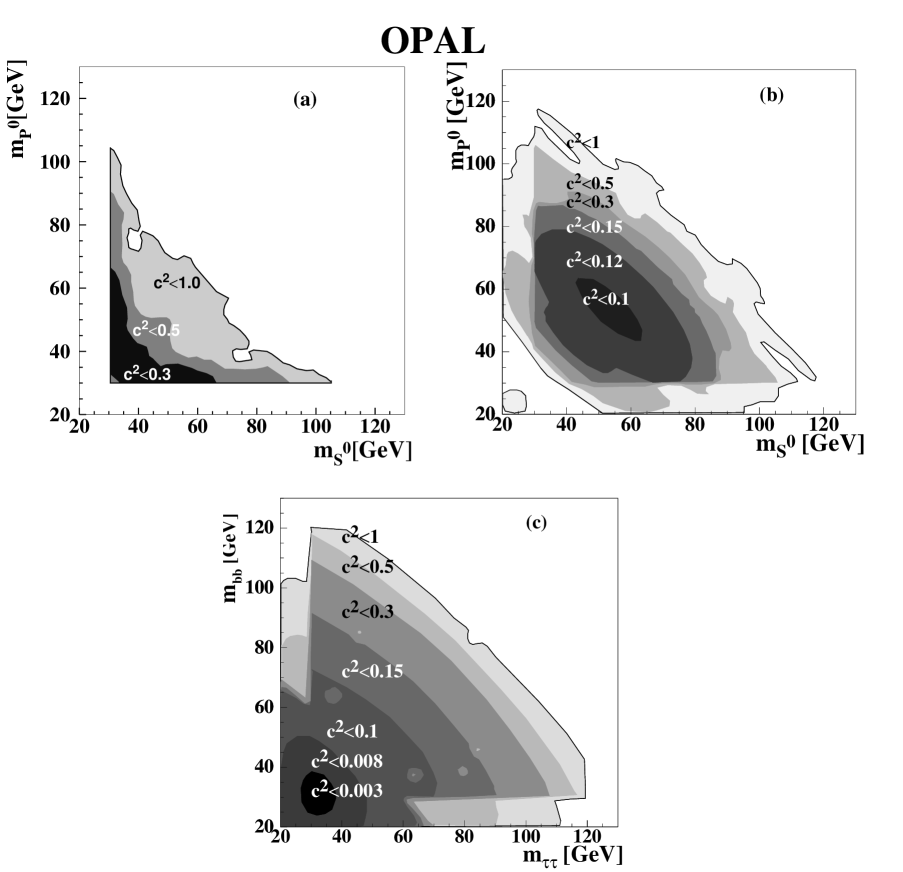
Figure 13: Upper limits at 95% CL for $c^{2}$ (a) for the S⁰P⁰$\rightarrow$$\mathrm{q}\bar{\mathrm{q}}$$\mathrm{q}\bar{\mathrm{q}}$, $\mathrm{g}\mathrm{g}$$\mathrm{q}\bar{\mathrm{q}}$ and $\mathrm{g}\mathrm{g}$$\mathrm{g}\mathrm{g}$ search channel assuming the hadronic branching ratio for both S⁰ and P⁰ to be 100%, (b) for the S⁰P⁰$\rightarrow$$\mathrm{b}\bar{\mathrm{b}}$$\mathrm{b}\bar{\mathrm{b}}$ search channel assuming the $\mathrm{b}\bar{\mathrm{b}}$ branching ratio for both S⁰ and P⁰ to be 100%, and (c) for the S⁰P⁰$\rightarrow$$\mathrm{b}\bar{\mathrm{b}}$$\tau^{+}\tau^{-}$ search channel assuming a 100% branching ratio for this final state. The invariant masses of the tau-lepton pair and b–jet pair in (c) are denoted by $m_{\tau\tau}$ and $m_{b\bar{b}}$, respectively. The iso-contour lines are at values of $c^{2}\leq 1.0$, 0.5 and 0.3 in (a), $c^{2}\leq 1.0$, 0.5, 0.3, 0.15, 0.12 and 0.1 in (b) and $c^{2}\leq 1.0$, 0.5, 0.3, 0.15, 0.1, 0.008 and 0.003 in (c), respectively.

7 Two Higgs Doublet Model interpretations

The interpretation of the searches for the neutral Higgs bosons in the 2HDM(II) is done by scanning the parameter space of the model. Every ($m_{\mathrm{h}}$, $m_{\mathrm{A}}$, $\tan\!\beta$, $\alpha$) point determines the production cross–section and the branching ratios to different final states. An updated version of the HZHA Monte Carlo generator [15] that includes the 2HDM(II) production cross–sections and branching ratios for Higgs decays has been used to scan the parameter space. This generator includes next-to-next-to-leading order QCD corrections and next-to-leading order electroweak corrections. The branching ratios obtained were cross–checked with the results of another generator  [41] in which QCD corrections are computed only up to next-to-leading order. The comparison showed good agreement between the results of the two programs.

The results of all the individual search channels at the studied centre–of–mass energies are combined statistically to constrain the 2HDM(II) parameter space. Although the flavour independent channels supply a unique way to investigate parameter space regions where the branching ratio $\mathrm{h}^{0}$$\rightarrow$$\mathrm{b}\bar{\mathrm{b}}$ or $\mathrm{A}^{0}$$\rightarrow$$\mathrm{b}\bar{\mathrm{b}}$ is highly suppressed (e.g., low $\alpha$ and $\tan\!\beta$ regions), they have a poor sensitivity with respect to the b–tagging channels outside these regions. The use of b–tagging information substantially reduces the background coming from $\mathrm{W}^{+}\mathrm{W}^{-}$ events and improves the sensitivity to observe Higgs bosons even in regions of the 2HDM(II) parameter space where only small branching ratios for $\mathrm{h}^{0}$$\rightarrow$$\mathrm{b}\bar{\mathrm{b}}$ are expected. The expected confidence level is calculated alternatively including only the b–tagged or non–b–tagged channels: for each parameter space point, either the flavour independent or the b–tagging analysis is then chosen for the extraction of the limits, depending on which provides the better expected confidence level.

The parameter space covered by the present study is:

• $1\leq\mbox{$m_{\mathrm{h}}$}\leq 100$ GeV, in steps of 1 GeV

• $5\leq\mbox{$m_{\mathrm{A}}$}\leq 100$ GeV, in steps of 1 GeV;
  $100\leq\mbox{$m_{\mathrm{A}}$}\leq 500$ GeV, in steps of 5 GeV;
  $0.5\leq\mbox{$m_{\mathrm{A}}$}\leq 2.0$ TeV, in steps of 0.5 TeV

• $0.4\leq\mbox{$\tan\!\beta$}\leq 58.0$, in steps of $1^{\circ}$ in $\beta$

• $\alpha=0,-\pi/8,-\pi/4,-3\pi/8$ and $-\pi/2$

The values of $\alpha$ are chosen to extend the analysis to the particular cases of maximal and minimal mixing in the neutral CP-even sector of the 2HDM(II) ($\alpha=-\pi/4$ and $-\pi/2$, respectively) and of BR($\mathrm{h}^{0}$$\rightarrow$$\mathrm{b}\bar{\mathrm{b}}$) = 0 ($\alpha=0$). A more complete picture of the model is obtained by studying two more intermediate values of $\alpha$. For $\tan\!\beta$ $<$ 0.4 radiative corrections become unstable. Below $m_{\mathrm{A}}$$\approx$ 5 GeV the direct search in the ${\mathrm{e}}^{+}{\mathrm{e}}^{-}$$\rightarrow$$\mathrm{h}^{0}$$\mathrm{A}^{0}$ channel cannot be included since the detection efficiency vanishes, and the constraint from the total $\mathrm{Z}^{0}$ width provides very limited exclusion since the contribution is too small. The other two free parameters of the model, $m_{\mathrm{H}}$ and $m_{\mathrm{H^{\pm}}}$, are not scanned in the present study. They are fixed at values above the kinematically accessible region at the present centre–of–mass energies at LEP2.

The production of any neutral low mass scalar particle in association with the $\mathrm{Z}^{0}$ was investigated in a previous OPAL publication  [42] and, for $m_{\mathrm{h}}$ $\leq$ 9.5 GeV, a mass-dependent upper limit on the Higgs boson production cross–section was obtained. This limit translates directly into an upper limit on the 2HDM(II) production cross–section for $m_{\mathrm{h}}$ below 9.5 GeV. Another powerful experimental constraint on extensions of the SM is the determination of the total width of the $\mathrm{Z}^{0}$ boson at LEP [40]. Any possible excess width obtained when subtracting the predicted SM width from the measured $\Gamma_{\mathrm{Z}}$ value can be used to place upper limits on the cross–section of $\mathrm{Z}^{0}$ decays into final states with $\mathrm{h}^{0}$ and $\mathrm{A}^{0}$ bosons  [43]. An expected increase of the partial width of the $\mathrm{Z}^{0}$ is evaluated for each scanned parameter space point in the 2HDM(II); if it is found to exceed the experimental limit, the point is excluded. The two constraints discussed above are treated together and are referred to as $\mathrm{Z}^{0}$ width in the rest of the paper, since for low $m_{\mathrm{h}}$ values most of the excluded regions are obtained from the constraints derived from $\Gamma_{\mathrm{Z}}$.

The direct searches for the process ${\mathrm{e}}^{+}{\mathrm{e}}^{-}$$\rightarrow$$\mathrm{h}^{0}$$\mathrm{Z}^{0}$  (${\mathrm{e}}^{+}{\mathrm{e}}^{-}$$\rightarrow$$\mathrm{h}^{0}$$\mathrm{A}^{0}$) in the $\mathrm{Z}^{0}$ data contribute mainly in the $m_{\mathrm{h}}$$\leq$ 50 GeV ($m_{\mathrm{h}}$$\leq$ 60 GeV) region. Since the flavour independent $\mathrm{h}^{0}$$\mathrm{Z}^{0}$ and $\mathrm{h}^{0}$$\mathrm{A}^{0}$  analyses have been performed in the mass regions $m_{\mathrm{h}}$$\geq$ 60 GeV (for the tau and missing energy channel, $m_{\mathrm{h}}$$\geq$ 30 GeV) and $m_{\mathrm{h}}$, $m_{\mathrm{A}}$$\geq$ 30 GeV, respectively, only b-tagging channels using higher energy data are applied below these masses; however these channels have no detection efficiency for $m_{\mathrm{h}}$$\leq$ 30 GeV. The flavour independent analyses provide exclusion for the whole $\tan\!\beta$ range and for the $\tan\!\beta$$<$1 regions for $\alpha=0$ and $\alpha=-\pi/8$, respectively. In Figures 14(a–e) the excluded regions in the ($m_{\mathrm{h}}$, $m_{\mathrm{A}}$) plane are shown for the five chosen values of $\alpha$, together with the calculated expected exclusion limits. A particular ($m_{\mathrm{h}}$, $m_{\mathrm{A}}$, $\alpha$) point is excluded at 95% CL if it is excluded for all scanned values of $\tan\!\beta$. Different domains of $\tan\!\beta$ are studied and described below: a) 0.4 $\leq$ $\tan\!\beta$$\leq$ 58.0 and b) 0.4 $\leq$ $\tan\!\beta$ $\leq$ 1.0 or 1.0 $<$ $\tan\!\beta$$\leq$ 58.0, for which enlarged excluded regions are obtained.

a) 0.4 $\leq$ $\tan\!\beta$$\leq$ 58.0 (darker grey area):

• The poor sensitivity of the $\mathrm{Z}^{0}$ channels below $m_{\mathrm{h}}$ $\lesssim$ 10 GeV causes a sharp cut in the exclusion plots at this $m_{\mathrm{h}}$ for $\alpha>-\pi/2$. The exclusion in this region is extracted from the total width of the $\mathrm{Z}^{0}$ boson, as explained above. Both the $\mathrm{h}^{0}$$\mathrm{Z}^{0}$ and $\mathrm{h}^{0}$$\mathrm{A}^{0}$ production processes contribute to the natural width of the $\mathrm{Z}^{0}$. While an excess, induced by the $\mathrm{h}^{0}$$\mathrm{Z}^{0}$ process, extends the exclusion region to any value of $m_{\mathrm{A}}$, the exclusion provided by the $\mathrm{h}^{0}$$\mathrm{A}^{0}$ process is kinematically limited to the region where $m_{\mathrm{A}}$ + $m_{\mathrm{h}}$ $\leq$ $m_{\mathrm{Z}}$. The contribution of the $\mathrm{h}^{0}$$\mathrm{Z}^{0}$ production cross–section to the $\mathrm{Z}^{0}$ width depends on the argument $(\beta-\alpha)$, and it becomes large enough for this process alone to provide exclusion in different $\tan\!\beta$ domains for the $\alpha$ values considered.

• For $\alpha$ = 0 and $-\pi/8$, most of the exclusion is provided by the channels at $\sqrt{s}$ = $m_{\mathrm{Z}}$, where no b–tagging was applied. In fact, the flavour independent analyses at $\sqrt{s}$  $\approx$ 189 GeV have a limited sensitivity because of the presence of the $\mathrm{W}^{+}\mathrm{W}^{-}$ background events. The line at $m_{\mathrm{h}}$ $\approx$ 57 GeV in Figure 14(b) is a result of the $\mathrm{Z}^{0}$ data kinematic constraint.

• The presence of candidates in the four–jet and $\tau^{+}\tau^{-}$ b-tagging $\mathrm{h}^{0}$$\mathrm{A}^{0}$ channels at $\sqrt{s}$ = 189 GeV at $m_{\mathrm{h}}$, $m_{\mathrm{A}}$ $\approx$ 80 GeV, due to the $\mathrm{W}^{+}\mathrm{W}^{-}$ background, is clearly reflected in Figure 14(c). The unexcluded region at ($m_{\mathrm{h}}$, $m_{\mathrm{A}}$) $\approx$ (60, 90) GeV in 14(d) is due to the presence of candidates in the four–jet b-tagging $\mathrm{h}^{0}$$\mathrm{A}^{0}$ channel.

• The shape of the exclusion plot in Figure 14(e) for $m_{\mathrm{h}}$ $<$ 35 GeV is related to the kinematical constraint on the $\mathrm{h}^{0}$$\mathrm{A}^{0}$ production in the $\mathrm{Z}^{0}$ data, which for $\alpha$ = $-\pi/2$ and large $\tan\!\beta$ is the only allowed process, since the $\mathrm{h}^{0}$$\mathrm{Z}^{0}$ production cross–section  vanishes  when  $\beta-\alpha\approx\pi$.  For $m_{\mathrm{h}}$ $>$ 35  GeV,  the  high  energy  data  open a  new

  

  
  

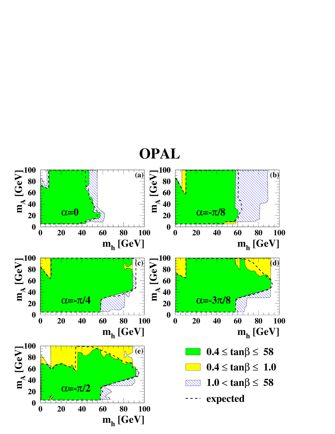
  Figure 14: Excluded regions in the ($m_{\mathrm{h}}$, $m_{\mathrm{A}}$) plane, (a)–(e), for $\alpha=$ 0, $-\pi/8$, $-\pi/4$, $-3\pi/8$ and $-\pi/2$, respectively, together with the expected exclusion limits. A particular ($m_{\mathrm{h}}$, $m_{\mathrm{A}}$, $\alpha$) point is excluded at 95% CL if it is excluded for all scanned values of $\tan\!\beta$. Three different domains of $\tan\!\beta$ are shown: the darker grey region is excluded for all values 0.4 $\leq$ $\tan\!\beta$$\leq$ 58.0; additional enlarged excluded regions are obtained constraining 0.4 $\leq$ $\tan\!\beta$ $\leq$ 1.0 (lighter grey area) or 1.0 $<$ $\tan\!\beta$$\leq$ 58.0 (hatched area). Expected exclusion limits are shown for 0.4 $\leq$ $\tan\!\beta$$\leq$ 58.0 (dashed line).

  kinematic region and are able to exclude large ($m_{\mathrm{h}}$, $m_{\mathrm{A}}$) areas, as can be seen by the sharp line in Figure 14(e).

• The ($m_{\mathrm{h}}$, $m_{\mathrm{A}}$) points below the semi-diagonal defined by $m_{\mathrm{h}}$$\geq$ 2$m_{\mathrm{A}}$, for which the process $\mathrm{h}^{0}$$\rightarrow$$\mathrm{A}^{0}$$\mathrm{A}^{0}$ is kinematically allowed, can only be excluded for $\tan\!\beta$ $>$ 0.5 values by the high energy channels. In fact, for very low values of $\tan\!\beta$ the branching ratio for $\mathrm{A}^{0}$$\rightarrow$$\mathrm{b}\bar{\mathrm{b}}$ vanishes, causing unexcluded regions in Figures 14(c), 14(d) and 14(e), which are excluded by the $\mathrm{Z}^{0}$ data flavour independent analyses below $m_{\mathrm{h}}$ $\approx$ 60 GeV.

b) 0.4 $\leq$ $\tan\!\beta$ $\leq$ 1.0 (lighter grey area) and 1.0 $<$ $\tan\!\beta$$\leq$ 58.0 (hatched area):

• As discussed above, as a consequence of the variation of the $\mathrm{h}^{0}$$\mathrm{Z}^{0}$ production cross–section with $\tan\!\beta$ in the $m_{\mathrm{h}}$ $<$ 10 GeV region, for $\alpha~{}=~{}-\pi/8$ in Figure 14(b), the $m_{\mathrm{h}}$ $>$ 7 GeV region is excluded for all values of $m_{\mathrm{A}}$ in the $\tan\!\beta$ $\leq$ 1.0 domain. For $\alpha$ = $-\pi/4$ and $-3/8\pi$, the $m_{\mathrm{h}}$ $<$ 10 GeV region is excluded for all values of $m_{\mathrm{A}}$ only in the $\tan\!\beta$ $\leq$ 1.0 domain.

• At $\alpha=0$ and $\alpha=-\pi/8$ and small values of $\tan\!\beta$ the production cross–section for the process ${\mathrm{e}}^{+}{\mathrm{e}}^{-}$$\rightarrow$$\mathrm{h}^{0}$$\mathrm{Z}^{0}$ is highly suppressed. For $m_{\mathrm{h}}$ $>$ 40 GeV, constraining $\tan\!\beta$ $>$ 1.0, larger excluded regions are obtained, as can be seen in Figures 14(a) and (b) (hatched areas).

• The presence of candidates in the four–jet and $\tau^{+}\tau^{-}$ b-tagging $\mathrm{h}^{0}$$\mathrm{A}^{0}$ channels at $\sqrt{s}$= 189 GeV at $m_{\mathrm{h}}$, $m_{\mathrm{A}}$ $\approx$ 80 GeV, corresponding to the $\mathrm{W}^{+}\mathrm{W}^{-}$ background, is clearly reflected in Figures 14(c), (d) and (e). For $\alpha$ = $-\pi/4$ and $\alpha$ = $-3\pi/8$ this region is unexcluded even for $\tan\!\beta$ $>1.0$, while for $\tan\!\beta$ $\leq$ 1.0 it is excluded due to a large expected production cross–section. For $\alpha$ = $-\pi/2$, the production cross-section becomes small and this domain is unexcluded for $\tan\!\beta$ $\leq$ 1.0, as can be seen in Figure 14(e).

In Figure 15 the excluded regions in the ($m_{\mathrm{h}}$, $m_{\mathrm{A}}$) plane independent of $\alpha$ are given together with the calculated expected exclusion limits. A particular ($m_{\mathrm{h}}$, $m_{\mathrm{A}}$) point is excluded at 95% CL if it is excluded for all scanned values of $\tan\!\beta$ and $\alpha$. Different domains of $\tan\!\beta$ are shown: 0.4 $\leq$ $\tan\!\beta$ $\leq$ 58.0 (darker grey area), 0.4 $\leq$ $\tan\!\beta$ $\leq$ 1.0 (lighter grey area) and 1.0 $<$ $\tan\!\beta$ $\leq$ 58.0 (hatched area), for which enlarged excluded regions are obtained. The rectangular region 1 $\lesssim$ $m_{\mathrm{h}}$ $\lesssim$ 44 GeV for 12 $\lesssim$ $m_{\mathrm{A}}$ $\lesssim$ 56 GeV is excluded at 95% CL independent of $\alpha$ and $\tan\!\beta$. The cross hatched region shows the exclusion provided by the constraints on the width of the $\mathrm{Z}^{0}$ common to all the scanned values of $\alpha$ and $\tan\!\beta$.

In Figures 16(a–e) the excluded regions in the ($\tan\!\beta$, $m_{\mathrm{h}}$) plane are shown for the five chosen values of $\alpha$, together with the calculated expected exclusion limits. A particular ($m_{\mathrm{h}}$, $\tan\!\beta$, $\alpha$) point is excluded at 95% CL if it is excluded for all scanned values of $m_{\mathrm{A}}$. There are two regions shown, the whole domain 5 GeV $\leq$ $m_{\mathrm{A}}$$\leq$ 2 TeV (darker grey area) and a restricted domain for which 5 $\leq$ $m_{\mathrm{A}}$ $\leq$ 60 GeV (lighter grey area). The exclusion contours for $m_{\mathrm{A}}$ $\leq$ 60 GeV are larger for all $\alpha$ values, and entirely contain the 5 GeV $\leq$ $m_{\mathrm{A}}$$\leq$ 2 TeV excluded areas.

In Figures 16(a) and (b), the unexcluded regions at low $\tan\!\beta$ and $m_{\mathrm{h}}$ $\leq$ 10 GeV reflect the behaviour in Figures 14(a) and (b) in the ($m_{\mathrm{h}}$, $m_{\mathrm{A}}$) plane for the same values of $\alpha$, for $m_{\mathrm{h}}$ $\leq$ 10 GeV and $m_{\mathrm{A}}$ $>$ 60 GeV. Similarly, the remaining three values of $\alpha$ show a complementary behaviour at large $\tan\!\beta$, reflecting the corresponding exclusion regions in the ($m_{\mathrm{h}}$, $m_{\mathrm{A}}$) plane, Figures 14(c), (d) and (e). In the $m_{\mathrm{A}}$ $\leq$ 60 GeV contours the same regions are obviously excluded. The $\mathrm{h}^{0}$$\mathrm{Z}^{0}$ production cross–section contribution to the $\mathrm{Z}^{0}$ width is not large enough to exclude the small region $\tan\!\beta$$>$ 10, 7 $\leq$ $m_{\mathrm{h}}$ $\leq$ 10 GeV in Figure 16(b). In Figure 16(e) the two unexcluded regions in the lighter grey area (5 $\leq$ $m_{\mathrm{A}}$ $\leq$ 60 GeV) at $m_{\mathrm{h}}$ $\approx$ 10 and 35 GeV are projections of the two regions unexcluded at the same $m_{\mathrm{h}}$ values in Figure 14(e) (darker grey area), for $m_{\mathrm{A}}$ $<$ 10 GeV and $m_{\mathrm{A}}$ $<$ 60 GeV, respectively.

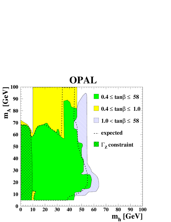
Figure 15: Excluded ($m_{\mathrm{A}}$, $m_{\mathrm{h}}$) region independent of $\alpha$, together with the expected exclusion limit. A particular ($m_{\mathrm{A}}$, $m_{\mathrm{h}}$) point is excluded at 95% CL if it is excluded for 0.4 $\leq$ $\tan\!\beta$ $\leq$ 58.0 (darker grey region), 0.4 $\leq$ $\tan\!\beta$ $\leq$ 1.0 (lighter grey region) and 1.0 $<$ $\tan\!\beta$ $\leq$ 58.0 (hatched region) for any $\alpha$. The cross–hatched region is excluded using constraints from $\Gamma_{\mathrm{Z}}$ only. Expected exclusion limits are shown as a dashed line.

In Figure 17 the excluded regions in the ($m_{\mathrm{A}}$, $\tan\!\beta$) plane are shown for different values of $\alpha$, together with the expected exclusion limits. A particular ($m_{\mathrm{A}}$, $\tan\!\beta$, $\alpha$) point is excluded at 95% CL if it is excluded for all scanned values of $m_{\mathrm{h}}$. There are three regions shown, corresponding to different $m_{\mathrm{h}}$ domains that are subsets of one another, namely: 1 $\leq$ $m_{\mathrm{h}}$ $\leq$ 90 GeV (darker grey area), 1 $\leq$ $m_{\mathrm{h}}$ $\leq$ 75 GeV (lighter grey area) and 1 $\leq$ $m_{\mathrm{h}}$ $\leq$ 60 GeV (hatched area). The lower the $m_{\mathrm{h}}$ upper value analysed, the larger the excluded ($m_{\mathrm{A}}$, $\tan\!\beta$) region. The unexcluded regions for $m_{\mathrm{A}}$ $>$ 60 GeV in Figures 17(b–e) gradually increase with decreasing $\alpha$. There is an exact correspondence between the largest excluded $\tan\!\beta$ value and the excluded regions at $m_{\mathrm{h}}$ $<$ 10 GeV in the ($m_{\mathrm{h}}$, $\tan\!\beta$)

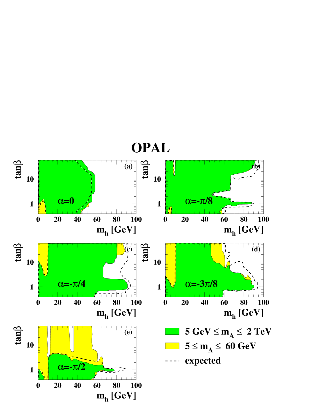
Figure 16: Excluded regions in the ($\tan\!\beta$, $m_{\mathrm{h}}$) plane, (a)–(e), for $\alpha$= 0, $-\pi/8$, $-\pi/4$, $-3\pi/8$ and $-\pi/2$, respectively, together with the expected exclusion limits. A particular ($m_{\mathrm{h}}$, $\tan\!\beta$, $\alpha$) point is excluded at 95% CL if it is excluded for all scanned values of $m_{\mathrm{A}}$. The two regions shown correspond to the whole domain 5 GeV $\leq$ $m_{\mathrm{A}}$$\leq$ 2 TeV (darker grey area) and a restricted domain for which 5 $\leq$ $m_{\mathrm{A}}$ $\leq$ 60 GeV (lighter grey area). The exclusion regions for $m_{\mathrm{A}}$ $\leq$ 60 GeV entirely contain the 5 GeV $\leq$ $m_{\mathrm{A}}$$\leq$ 2 TeV excluded areas. Expected exclusion limits are shown for 5 GeV $\leq$ $m_{\mathrm{A}}$$\leq$ 2 TeV (dashed line).

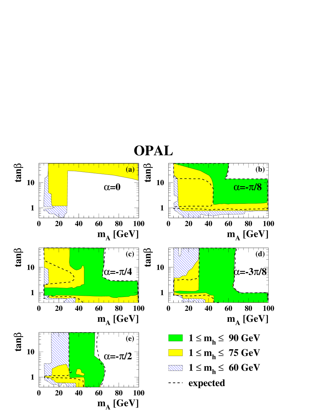
Figure 17: Excluded regions in the ($m_{\mathrm{A}}$, $\tan\!\beta$) plane, (a)–(e), for $\alpha$= 0, $-\pi/8$, $-\pi/4$, $-3\pi/8$ and $-\pi/2$ respectively, together with the calculated expected exclusion limits. A particular ($m_{\mathrm{A}}$, $\tan\!\beta$, $\alpha$) point is excluded at 95% CL if it is excluded for all scanned values of $m_{\mathrm{h}}$. The three contours correspond to 1 $\leq$ $m_{\mathrm{h}}$ $\leq$ 90 GeV (darker grey area), 1 $\leq$ $m_{\mathrm{h}}$ $\leq$ 75 GeV (lighter grey area) and 1 $\leq$ $m_{\mathrm{h}}$ $\leq$ 60 GeV (hatched area). Expected exclusion limits are shown for 1 $\leq$ $m_{\mathrm{h}}$ $\leq$ 90 GeV (dashed line).

projections in Figures 16(b–e). The line at $m_{\mathrm{A}}$ $\approx$ 30 GeV for $\tan\!\beta$ $>$ 1.0 in the exclusion region for $m_{\mathrm{h}}$ $<$ 90 GeV in Figures 17(d) and (e) corresponds to the horizontal line at $m_{\mathrm{A}}$ = 30 GeV in the $\tan\!\beta$ $>$ 1.0 contour in Figures 14(d) and (e). The small island at 35 $<$ $m_{\mathrm{A}}$ $<$ 39 GeV and 1.0 $<$ $\tan\!\beta$ $<$ 2.0 in Figure 17(e) is the reflection of a candidate in the $\mathrm{h}^{0}$$\mathrm{A}^{0}$$\rightarrow$$\tau^{+}\tau^{-}$$\mathrm{b}\bar{\mathrm{b}}$ channel at $\sqrt{s}$= 183 GeV with $m_{\mathrm{A}}$ $\approx$ 37 GeV and $m_{\mathrm{h}}$ $\approx$ 80 GeV.

8 Conclusions

A general analysis of the 2HDM(II) with no CP–violation and no extra particles besides those of the SM and the five Higgs bosons has been performed for the first time. Large areas of the parameter space of the model have been scanned. In the scanning procedure the dependence of the production cross–sections and branching ratios on the angles $\alpha$ and $\beta$, calculated with next-to-next-to-leading order QCD corrections and next-to-leading order electroweak corrections, has been considered.

In addition to the standard OPAL b–tagging analyses, new flavour independent channels for both the Higgs–strahlung process, ${\mathrm{e}}^{+}{\mathrm{e}}^{-}$$\rightarrow$$\mathrm{h}^{0}$$\mathrm{Z}^{0}$, and the pair–production process, ${\mathrm{e}}^{+}{\mathrm{e}}^{-}$$\rightarrow$$\mathrm{h}^{0}$$\mathrm{A}^{0}$, have been analysed, providing access to regions of parameter space in the 2HDM(II) where $\mathrm{h}^{0}$ and $\mathrm{A}^{0}$ are expected to decay predominantly into up–type light quarks and gluons (e.g. $\alpha\approx 0$).

OPAL data collected at $\sqrt{s}$ $\approx$ $m_{\mathrm{Z}}$, 183 and 189 GeV have been interpreted both in the context of the 2HDM(II) and in a model–independent approach where both SM branching ratios and 100% hadronic branching ratios were assumed.

The 2HDM(II) parameter space scan, for 1 $\leq$ $m_{\mathrm{h}}$ $\leq$ 100 GeV, 5 GeV $\leq$ $m_{\mathrm{A}}$ $\leq$ 2 TeV, $-\pi/2\leq\alpha\leq 0$ and $0.4\leq\mbox{$\tan\!\beta$}\leq 58.0$, leads to large regions excluded at the 95% CL in the ($m_{\mathrm{h}}$, $m_{\mathrm{A}}$) plane as well as in the ($m_{\mathrm{h}}$, $\tan\!\beta$) and ($m_{\mathrm{A}}$, $\tan\!\beta$) projections. The region 1 $\lesssim$ $m_{\mathrm{h}}$ $\lesssim$ 44 GeV and 12 $\lesssim$ $m_{\mathrm{A}}$ $\lesssim$ 56 GeV is excluded at 95% CL independent of $\alpha$ and $\tan\!\beta$ within the scanned parameter space.

In the model–independent approach for ${\mathrm{e}}^{+}{\mathrm{e}}^{-}$$\rightarrow$ S⁰$\mathrm{Z}^{0}$, lower bounds at 95% CL are obtained for $s^{2}=$ 1 of 91 GeV assuming SM branching ratios and 75 GeV assuming 100% hadronic branching ratios. In the case of the generic processes S⁰P⁰ $\rightarrow$ $\mathrm{b}\bar{\mathrm{b}}$$\mathrm{b}\bar{\mathrm{b}}$ and S⁰P${}^{0}~{}\rightarrow$ $\mathrm{b}\bar{\mathrm{b}}$ $\tau^{+}\tau^{-}$, a lower bound at 95% CL of $m_{\mathrm{S}}=m_{\mathrm{P}}>78$ GeV is extracted along the diagonal for $c^{2}=1$ assuming 100% branching ratios for the individual final states, while assuming the S⁰ P⁰ hadronic branching ratios to be 100% gives $m_{\mathrm{S}}=m_{\mathrm{P}}>61$ GeV.

Acknowledgements:

We particularly wish to thank the SL Division for the efficient operation of the LEP accelerator at all energies and for their continuing close cooperation with our experimental group. We thank our colleagues from CEA, DAPNIA/SPP, CE-Saclay for their efforts over the years on the time-of-flight and trigger systems which we continue to use. In addition to the support staff at our own institutions we are pleased to acknowledge the
Department of Energy, USA,
National Science Foundation, USA,
Particle Physics and Astronomy Research Council, UK,
Natural Sciences and Engineering Research Council, Canada,
Israel Science Foundation, administered by the Israel Academy of Science and Humanities,
Minerva Gesellschaft,
Benoziyo Center for High Energy Physics,
Japanese Ministry of Education, Science and Culture (the Monbusho) and a grant under the Monbusho International Science Research Program,
Japanese Society for the Promotion of Science (JSPS),
German Israeli Bi-national Science Foundation (GIF),
Bundesministerium für Bildung und Forschung, Germany,
National Research Council of Canada,
Research Corporation, USA,
Hungarian Foundation for Scientific Research, OTKA T-029328, T023793 and OTKA F-023259.

References

- [1] P. W. Higgs, Phys. Lett. 12, 132 (1964).
- [2] F. Englert and R. Brout, Phys. Rev. Lett. 13, 321 (1964).
- [3] G.S. Guralnik, C.R. Hagen and T.W.B. Kibble, Phys. Rev. Lett. 13, 585 (1964).
- [4] W. Hollik, Z. Phys C32, 291 (1986).
- [5] W. Hollik, Z. Phys C37, 569 (1988).
- [6] J.F. Gunion, H.E Haber, G.L. Kane and S. Dawson, The Higgs Hunter’s Guide, Addison-Wesley Publishing Company, 1990.
- [7] P. Fayet, Nucl. Phys. B90, 104 (1975).
- [8] OPAL Collaboration, K. Ahmet et al., Nucl. Instr. and Meth. A305, 275 (1991).
- [9] S. Anderson et al., Nucl. Instr. and Meth. A403, 326 (1998).
- [10] B.E. Anderson et al., IEEE Transactions on Nuclear Science 41, 845 (1994).
- [11] OPAL Collaboration, K. Ackerstaff et al., Phys. Lett. B391, 221 (1997).
- [12] OPAL Collaboration, R. Akers et al., Phys. Lett. B327, 397 (1994).
-
[13]
N. Brown and W.J. Stirling, Phys. Lett., B252,657 (1990);
S. Catani et al., Phys. Lett., B269, 432 (1991);
S. Bethke, Z. Kunszt, D. Soper and W.J. Stirling, Nucl. Phys., B370, 310 (1992);
N. Brown and W.J. Stirling, Z. Phys., C53, 629 (1992). - [14] OPAL Collaboration, K. Ackerstaff et al., Eur. Phys. J. C2, 213 (1998).
- [15] HZHA generator: P. Janot, G. Ganis, Physics at LEP2, CERN 96-01 (1996) Vol. 2, 309.
- [16] T. Sjöstrand, Comp. Phys. Comm. 82, 74 (1994).
- [17] J. Fujimoto et al., Comp. Phys. Comm. 100, 128 (1997).
- [18] F.A. Berends, R. Pittau and R. Kleiss, Comp. Phys. Comm. 85, 437 (1995).
- [19] BHWIDE generator: S. Jadak, W. Placzek, B. F. L. Ward, Physics at LEP2, CERN 96-01 (1996) Vol. 2, 286; UTHEP–95–1001.
- [20] S. Jadach, B.F.L. Ward, and Z. Wa̧s, Comp. Phys. Comm. 79, 503 (1994).
- [21] R. Engel and J. Ranft, Phys. Rev. D54, 4244 (1996).
- [22] G. Marchesini et al., Comp. Phys. Comm. 67, 465 (1992).
- [23] J.A.M. Vermaseren, Nucl. Phys. B229, 347 (1983).
- [24] OPAL Collaboration, G. Alexander et al., Z. Phys C69, 543 (1996).
- [25] J. Allison et al., Nucl. Instr. and Meth. A317, 47 (1992).
- [26] OPAL Collaboration, R. Akers et al., Phys. Lett. B327, 397 (1994).
- [27] OPAL Collaboration, R. Akers et al., Z. Phys. C64, 1 (1994).
- [28] OPAL Collaboration, G.Alexander et al., Z. Phys. C73, 189 (1997).
- [29] OPAL Collaboration, K. Ackerstaff et al., Eur.Phys.J. C7, 407 (1999).
- [30] OPAL Collaboration, K. Ackerstaff et al., Eur. Phys. J. C12, 567 (2000).
- [31] F. Berends and R. Kleiss, Nucl. Phys. B260, 32 (1985).
- [32] OPAL Collaboration, K. Ackerstaff et al., Eur. Phys. J. C1, 425 (1998).
- [33] OPAL Collaboration, G. Abbiendi et al., QCD Studies with Annihilation Data at 172–189 GeV, CERN-EP-99-178, to be published in Eur. Phys. J. C. Note that .
- [34] S. Catani and M. Seymour, Phys. Lett. B378, 287 (1996).
- [35] OPAL Collaboration, K. Ackerstaff et al., Eur. Phys. J. C2, 441 (1998).
-
[36]
G. Hanson et al., Phys. Rev. Lett. 35, 1609 (1975);
G. Parisi, Phys. Lett., B74, 65 (1978). - [37] OPAL Collaboration, G. Abbiendi et al., Eur.Phys.J. C8, 191 (1999).
- [38] OPAL Collaboration, G. Abbiendi et al., Eur. Phys. J. C8, 191 (1999).
- [39] OPAL Collaboration, K. Ackerstaff et al., Eur. Phys. J. C5, 19 (1998).
- [40] D. Schaile, Fortschritte der Physik 42, 429 (1994).
- [41] M. Krawczyk, J. Zochowski and P. Mättig, Eur. Phys. J. C8, 495 (1999).
- [42] OPAL Collaboration, P. D. Acton et al., Phys. Lett. B268, 122 (1991).
- [43] OPAL Collaboration, K. Ackerstaff et al., Eur. Phys. J. C5, 19 (1998).