EUROPEAN ORGANISATION FOR NUCLEAR RESEARCH

The OPAL Collaboration

G. Abbiendi², K. Ackerstaff⁸, C. Ainsley⁵, P.F. Akesson³, G. Alexander²², J. Allison¹⁶, K.J. Anderson⁹, S. Arcelli¹⁷, S. Asai²³, S.F. Ashby¹, D. Axen²⁷, G. Azuelos^18,a, I. Bailey²⁶, A.H. Ball⁸, E. Barberio⁸, R.J. Barlow¹⁶, S. Baumann³, J. Bechtluft¹⁴, T. Behnke²⁵, K.W. Bell²⁰, G. Bella²², A. Bellerive⁹, S. Bentvelsen⁸, S. Bethke^14,i, O. Biebel^14,i, I.J. Bloodworth¹, P. Bock¹¹, J. Böhme^14,h, O. Boeriu¹⁰, D. Bonacorsi², M. Boutemeur³¹, S. Braibant⁸, P. Bright-Thomas¹, L. Brigliadori², R.M. Brown²⁰, H.J. Burckhart⁸, J. Cammin³, P. Capiluppi², R.K. Carnegie⁶, A.A. Carter¹³, J.R. Carter⁵, C.Y. Chang¹⁷, D.G. Charlton^1,b, C. Ciocca², P.E.L. Clarke¹⁵, E. Clay¹⁵, I. Cohen²², O.C. Cooke⁸, J. Couchman¹⁵, C. Couyoumtzelis¹³, R.L. Coxe⁹, M. Cuffiani², S. Dado²¹, G.M. Dallavalle², S. Dallison¹⁶, A. de Roeck⁸, P. Dervan¹⁵, K. Desch²⁵, B. Dienes^30,h, M.S. Dixit⁷, M. Donkers⁶, J. Dubbert³¹, E. Duchovni²⁴, G. Duckeck³¹, I.P. Duerdoth¹⁶, P.G. Estabrooks⁶, E. Etzion²², F. Fabbri², M. Fanti², L. Feld¹⁰, P. Ferrari¹², F. Fiedler⁸, I. Fleck¹⁰, M. Ford⁵, A. Frey⁸, A. Fürtjes⁸, D.I. Futyan¹⁶, P. Gagnon¹², J.W. Gary⁴, G. Gaycken²⁵, C. Geich-Gimbel³, G. Giacomelli², P. Giacomelli⁸, D. Glenzinski⁹, J. Goldberg²¹, C. Grandi², K. Graham²⁶, E. Gross²⁴, J. Grunhaus²², M. Gruwé²⁵, P.O. Günther³, C. Hajdu²⁹, G.G. Hanson¹², M. Hansroul⁸, M. Hapke¹³, K. Harder²⁵, A. Harel²¹, C.K. Hargrove⁷, M. Harin-Dirac⁴, A. Hauke³, M. Hauschild⁸, C.M. Hawkes¹, R. Hawkings²⁵, R.J. Hemingway⁶, C. Hensel²⁵, G. Herten¹⁰, R.D. Heuer²⁵, M.D. Hildreth⁸, J.C. Hill⁵, A. Hocker⁹, K. Hoffman⁸, R.J. Homer¹, A.K. Honma⁸, D. Horváth^29,c, K.R. Hossain²⁸, R. Howard²⁷, P. Hüntemeyer²⁵, P. Igo-Kemenes¹¹, K. Ishii²³, F.R. Jacob²⁰, A. Jawahery¹⁷, H. Jeremie¹⁸, C.R. Jones⁵, P. Jovanovic¹, T.R. Junk⁶, N. Kanaya²³, J. Kanzaki²³, G. Karapetian¹⁸, D. Karlen⁶, V. Kartvelishvili¹⁶, K. Kawagoe²³, T. Kawamoto²³, R.K. Keeler²⁶, R.G. Kellogg¹⁷, B.W. Kennedy²⁰, D.H. Kim¹⁹, K. Klein¹¹, A. Klier²⁴, T. Kobayashi²³, M. Kobel³, T.P. Kokott³, S. Komamiya²³, R.V. Kowalewski²⁶, T. Kress⁴, P. Krieger⁶, J. von Krogh¹¹, T. Kuhl³, M. Kupper²⁴, P. Kyberd¹³, G.D. Lafferty¹⁶, H. Landsman²¹, D. Lanske¹⁴, J. Lauber¹⁵, I. Lawson²⁶, J.G. Layter⁴, A. Leins³¹, D. Lellouch²⁴, J. Letts¹², L. Levinson²⁴, R. Liebisch¹¹, J. Lillich¹⁰, B. List⁸, C. Littlewood⁵, A.W. Lloyd¹, S.L. Lloyd¹³, F.K. Loebinger¹⁶, G.D. Long²⁶, M.J. Losty⁷, J. Lu²⁷, J. Ludwig¹⁰, A. Macchiolo¹⁸, A. Macpherson²⁸, W. Mader³, M. Mannelli⁸, S. Marcellini², T.E. Marchant¹⁶, A.J. Martin¹³, J.P. Martin¹⁸, G. Martinez¹⁷, T. Mashimo²³, P. Mättig²⁴, W.J. McDonald²⁸, J. McKenna²⁷, T.J. McMahon¹, R.A. McPherson²⁶, F. Meijers⁸, P. Mendez-Lorenzo³¹, F.S. Merritt⁹, H. Mes⁷, A. Michelini², S. Mihara²³, G. Mikenberg²⁴, D.J. Miller¹⁵, W. Mohr¹⁰, A. Montanari², T. Mori²³, K. Nagai⁸, I. Nakamura²³, H.A. Neal^12,f, R. Nisius⁸, S.W. O’Neale¹, F.G. Oakham⁷, F. Odorici², H.O. Ogren¹², A. Oh⁸, A. Okpara¹¹, M.J. Oreglia⁹, S. Orito²³, G. Pásztor^8,j, J.R. Pater¹⁶, G.N. Patrick²⁰, J. Patt¹⁰, P. Pfeifenschneider¹⁴, J.E. Pilcher⁹, J. Pinfold²⁸, D.E. Plane⁸, B. Poli², J. Polok⁸, O. Pooth⁸, M. Przybycień^8,d, A. Quadt⁸, C. Rembser⁸, H. Rick⁴, S.A. Robins²¹, N. Rodning²⁸, J.M. Roney²⁶, S. Rosati³, K. Roscoe¹⁶, A.M. Rossi², Y. Rozen²¹, K. Runge¹⁰, O. Runolfsson⁸, D.R. Rust¹², K. Sachs⁶, T. Saeki²³, O. Sahr³¹, E.K.G. Sarkisyan²², C. Sbarra²⁶, A.D. Schaile³¹, O. Schaile³¹, P. Scharff-Hansen⁸, S. Schmitt¹¹, M. Schröder⁸, M. Schumacher²⁵, C. Schwick⁸, W.G. Scott²⁰, R. Seuster^14,h, T.G. Shears⁸, B.C. Shen⁴, C.H. Shepherd-Themistocleous⁵, P. Sherwood¹⁵, G.P. Siroli², A. Skuja¹⁷, A.M. Smith⁸, G.A. Snow¹⁷, R. Sobie²⁶, S. Söldner-Rembold^10,e, S. Spagnolo²⁰, M. Sproston²⁰, A. Stahl³, K. Stephens¹⁶, K. Stoll¹⁰, D. Strom¹⁹, R. Ströhmer³¹, B. Surrow⁸, S.D. Talbot¹, S. Tarem²¹, R.J. Taylor¹⁵, R. Teuscher⁹, M. Thiergen¹⁰, J. Thomas¹⁵, M.A. Thomson⁸, E. Torrence⁹, S. Towers⁶, T. Trefzger³¹, I. Trigger⁸, Z. Trócsányi^30,g, E. Tsur²², M.F. Turner-Watson¹, I. Ueda²³, P. Vannerem¹⁰, M. Verzocchi⁸, H. Voss⁸, J. Vossebeld⁸, D. Waller⁶, C.P. Ward⁵, D.R. Ward⁵, J.J. Ward⁸, P.M. Watkins¹, A.T. Watson¹, N.K. Watson¹, P.S. Wells⁸, T. Wengler⁸, N. Wermes³, D. Wetterling¹¹ J.S. White⁶, G.W. Wilson¹⁶, J.A. Wilson¹, T.R. Wyatt¹⁶, S. Yamashita²³, V. Zacek¹⁸, D. Zer-Zion⁸

¹School of Physics and Astronomy, University of Birmingham, Birmingham B15 2TT, UK
²Dipartimento di Fisica dell’ Università di Bologna and INFN, I-40126 Bologna, Italy
³Physikalisches Institut, Universität Bonn, D-53115 Bonn, Germany
⁴Department of Physics, University of California, Riverside CA 92521, USA
⁵Cavendish Laboratory, Cambridge CB3 0HE, UK
⁶Ottawa-Carleton Institute for Physics, Department of Physics, Carleton University, Ottawa, Ontario K1S 5B6, Canada
⁷Centre for Research in Particle Physics, Carleton University, Ottawa, Ontario K1S 5B6, Canada
⁸CERN, European Organisation for Nuclear Research, CH-1211 Geneva 23, Switzerland
⁹Enrico Fermi Institute and Department of Physics, University of Chicago, Chicago IL 60637, USA
¹⁰Fakultät für Physik, Albert Ludwigs Universität, D-79104 Freiburg, Germany
¹¹Physikalisches Institut, Universität Heidelberg, D-69120 Heidelberg, Germany
¹²Indiana University, Department of Physics, Swain Hall West 117, Bloomington IN 47405, USA
¹³Queen Mary and Westfield College, University of London, London E1 4NS, UK
¹⁴Technische Hochschule Aachen, III Physikalisches Institut, Sommerfeldstrasse 26-28, D-52056 Aachen, Germany
¹⁵University College London, London WC1E 6BT, UK
¹⁶Department of Physics, Schuster Laboratory, The University, Manchester M13 9PL, UK
¹⁷Department of Physics, University of Maryland, College Park, MD 20742, USA
¹⁸Laboratoire de Physique Nucléaire, Université de Montréal, Montréal, Quebec H3C 3J7, Canada
¹⁹University of Oregon, Department of Physics, Eugene OR 97403, USA
²⁰CLRC Rutherford Appleton Laboratory, Chilton, Didcot, Oxfordshire OX11 0QX, UK
²¹Department of Physics, Technion-Israel Institute of Technology, Haifa 32000, Israel
²²Department of Physics and Astronomy, Tel Aviv University, Tel Aviv 69978, Israel
²³International Centre for Elementary Particle Physics and Department of Physics, University of Tokyo, Tokyo 113-0033, and Kobe University, Kobe 657-8501, Japan
²⁴Particle Physics Department, Weizmann Institute of Science, Rehovot 76100, Israel
²⁵Universität Hamburg/DESY, II Institut für Experimental Physik, Notkestrasse 85, D-22607 Hamburg, Germany
²⁶University of Victoria, Department of Physics, P O Box 3055, Victoria BC V8W 3P6, Canada
²⁷University of British Columbia, Department of Physics, Vancouver BC V6T 1Z1, Canada
²⁸University of Alberta, Department of Physics, Edmonton AB T6G 2J1, Canada
²⁹Research Institute for Particle and Nuclear Physics, H-1525 Budapest, P O Box 49, Hungary
³⁰Institute of Nuclear Research, H-4001 Debrecen, P O Box 51, Hungary
³¹Ludwigs-Maximilians-Universität München, Sektion Physik, Am Coulombwall 1, D-85748 Garching, Germany


^a and at TRIUMF, Vancouver, Canada V6T 2A3
^b and Royal Society University Research Fellow
^c and Institute of Nuclear Research, Debrecen, Hungary
^d and University of Mining and Metallurgy, Cracow
^e and Heisenberg Fellow
^f now at Yale University, Dept of Physics, New Haven, USA
^g and Department of Experimental Physics, Lajos Kossuth University, Debrecen, Hungary
^h and MPI München
ⁱ now at MPI für Physik, 80805 München
^j and Research Institute for Particle and Nuclear Physics, Budapest, Hungary.

1 Introduction

The measurement of the hadronic photon structure function $\mbox{$F_{2}^{\gamma}$}(x,\mbox{$Q^{2}$})$ is a classic test of QCD predictions [1, 2, 3]. The structure function of the photon differs from that of the proton because the photon can couple directly to quark charges, as well as fluctuate into a hadronic state. The value of $F_{2}^{\mbox{\tiny proton}}(x,Q^{2})$ exhibits a clear rise towards low values of Bjorken $x$ [5, 4]. Some theoretical models predict a similar rise in the photon structure function [6, 7, 8], while other models do not require such a rise [9]. Experimentally, a rise at low-$x$ in the photon structure function has neither been observed nor excluded [10, 11, 12, 13, 14, 15, 16, 17, 18, 19]. The photon structure function is studied at LEP using samples of events of the type $\mbox{$\rm e^{+}e^{-}$}\rightarrow\mbox{$\rm e^{+}e^{-}$}\mbox{$\gamma^{\star}\gamma$}\rightarrow\mbox{$\rm e^{+}e^{-}$}+\mbox{hadrons}$. The analysis presented here uses single-tagged events (from here on referred to as $\gamma^{\star}\gamma$ events), which means that only one of the scattered beam electrons is observed in the detector. These events can be regarded as deep inelastic scattering of an electron off a quasi-real target photon, and the flux of quasi-real photons can be calculated using the equivalent photon approximation [1]. Figure 1 shows a diagram of this reaction, in which $k$ is the four-vector of the incoming electron which radiates the virtual photon, and $q$ and $p$ are the four-vectors of the virtual photon and the quasi-real photon, respectively. The symbol ${\rm f}_{\rm q,\gamma}(x,\mbox{$Q^{2}$})$ represents the parton densities of the quasi-real photon.

Figure 1: Deep inelastic electron-photon scattering.

The cross-section for deep inelastic electron-photon scattering can be written in terms of structure functions as [3]

$$\frac{\mbox{d}^{2}\sigma_{\rm e\gamma\rightarrow eX}}{\mbox{d}x\mbox{d}Q^{2}}=\frac{2\pi\mbox{$\mbox{$\alpha$ }^{2}$}}{x\,Q^{4}}\left[\left(1+(1-y)^{2}\right)\mbox{$\mbox{$F_{2}^{\gamma}$}(x,\mbox{$Q^{2}$})$}-y^{2}\mbox{$\mbox{$F_{\rm L}^{\gamma}$}(x,\mbox{$Q^{2}$})$}\right]$$ (1)

where $\mbox{$Q^{2}$}=-q^{2}$ is the negative value of the four-momentum squared of the virtual probe photon, $\alpha$  is the fine structure constant and $x$ and $y$ are the usual dimensionless deep inelastic scattering variables, defined by

$$x=\frac{\mbox{$Q^{2}$}}{2p\cdot q},\ y=\frac{p\cdot q}{p\cdot k}.$$ (2)

In the kinematic region studied in this paper, $y^{2}\ll 1$, so the contribution from the longitudinal photon structure function $F_{\rm L}^{\gamma}$ in Equation 1 is neglected.

In contrast to measurements of the proton structure function, here the energy of the target particle is not known. In consequence, the kinematics cannot be fully determined without measuring the hadronic final state, which is only partially observed in the detector. This leads to a dependence of the $F_{2}^{\gamma}$ measurement on Monte Carlo modelling of the hadronic final state, which enters when an unfolding process is used to relate the visible distributions to the underlying $x$ distribution.

The analysis presented here uses OPAL data collected during the years 1993–1995, 1997 and 1998, at $\rm e^{+}e^{-}$ centre-of-mass energies of 91 $\rm GeV$ (LEP1), and 183 $\rm GeV$ and 189 $\rm GeV$ (LEP2). This is the first OPAL measurement of the four-flavour photon structure function using the 183 $\rm GeV$ and 189 $\rm GeV$ data, though the charm contribution to $F_{2}^{\gamma}$ has already been measured [20]. In this analysis new Monte Carlo programs and improved unfolding methods have been introduced, which are also used in the re-analysis of the LEP1 data.

2 The OPAL detector

The OPAL detector is described in detail elsewhere [21]; only the subdetectors which are most relevant for this analysis, namely the low angle electromagnetic calorimeters and the tracking devices, are detailed below. The OPAL detector has a uniform magnetic field of 0.435 T along the beam direction throughout the central tracking region, with electromagnetic and hadronic calorimetry and muon chambers outside the coil.

The forward detectors (FD) cover the $\theta$ region from 60 to 140 mrad at each end of the OPAL detector. They consist of cylindrical lead-scintillator calorimeters with a depth of 24 radiation lengths ($X_{0}$) divided azimuthally into 16 segments. The energy resolution for electromagnetic showers is $18\%/\sqrt{E}$, where $E$ is in $\rm GeV$. An array of three planes of proportional tubes buried in the calorimeter at a depth of 4 $X_{0}$ provides a precise shower position measurement, with a typical resolution of 3–4 mm, corresponding to 2.5 mrad in $\theta$, and less than 3.5 mrad in $\phi$.

The small-angle silicon tungsten luminometer (SW) covered the region in $\theta$ from 25 to 60 mrad from 1993–1995. For LEP2 running, a radiation shield was installed which moved the lower edge of the useful SW acceptance to 33 mrad. The SW detector contains 19 layers of silicon alternating with tungsten. Each of the 16 azimuthal wedges is divided into 64 pads for positional measurement. The energy resolution of the SW detector is about $24\%/\sqrt{E}$ at LEP1 energies, and about $6\%$ at LEP2.

Charged particles are detected by a silicon microvertex detector, a drift chamber vertex detector, and a jet chamber. Outside the jet chamber, but still inside the magnetic field, lies a layer of drift chambers whose purpose is to improve the track reconstruction in the $z$-coordinate. The resolution of the transverse momentum for charged particles is $\sigma_{p_{\rm t}}/p_{\rm t}=\sqrt{0.02^{2}+(0.0015\,\mbox{$p_{\rm t}$})^{2}}$ for $\mbox{$|\cos\theta|$}<0.7$ , where $p_{\rm t}$ is in GeV, and degrades for higher values of $|\cos\theta|$. Tracks are accepted up to a limit of $\mbox{$|\cos\theta|$}<0.9622$.

Both ends of the OPAL detector are equipped with electromagnetic endcap calorimeters covering the range from 200 to 630 mrad in polar angle. They are homogeneous devices composed of arrays of lead-glass blocks of $9.2\times 9.2$ cm² cross-section and typically 22 $X_{0}$ in depth, giving good shower containment. In the central region, outside the solenoid, is the electromagnetic barrel calorimeter of similar construction.

The deep inelastic scattering events are triggered with high efficiency by the large energy deposits of the scattered electron in the forward calorimeters (FD and SW) and by charged particles seen in the tracking devices.

3 Kinematics and data selection

To measure $\mbox{$F_{2}^{\gamma}$}(x,\mbox{$Q^{2}$})$, the distribution of events in $x$ and $Q^{2}$ is needed. These variables, illustrated in Figure 1, are related to the experimentally measurable quantities

$$\mbox{$Q^{2}$}=2\,\mbox{$E_{\rm b}$}\,\mbox{$E_{\rm tag}$}\,(1-\cos\mbox{$\theta_{\rm tag}$})$$ (3)

and

$$x=\frac{\mbox{$Q^{2}$}}{\mbox{$Q^{2}$}+W^{2}+\mbox{$P^{2}$}}$$ (4)

where $E_{\rm b}$ is the energy of the beam electrons, $E_{\rm tag}$ and $\theta_{\rm tag}$ are the energy and polar angle of the deeply inelastically scattered (or ‘tagged’) electron, $W^{2}$ is the invariant mass squared of the hadronic final state and $\mbox{$P^{2}$}=-p^{2}$ is the negative value of the virtuality squared of the quasi-real photon. The requirement that the associated electron is not seen in the detector ensures that $\mbox{$P^{2}$}\ll\mbox{$Q^{2}$}$, so $P^{2}$ is neglected when calculating $x$ from Equation 4. The electron mass is neglected throughout.

Three samples of events are studied in this analysis, classified according to the centre-of-mass energy and the subdetector in which the tagged electron is observed. Data from LEP1 are used, with $\rm e^{+}e^{-}$ centre-of-mass energies close to the $\rm Z^{0}$ mass, as well as LEP2 data with centre-of-mass energies of 183 $\rm GeV$ and 189 $\rm GeV$. Electrons are tagged using the SW detector at all centre-of-mass energies, since accessing the lowest possible $x$ region requires measuring the electrons scattered at the lowest possible angles. The FD is only used for the LEP1 data, to provide a sample in the same range of $Q^{2}$ as the LEP2 sample, but using a different subdetector for tagging the scattered electron. The three samples used are termed LEP1 SW, LEP1 FD and LEP2 SW. Each sample is further split into two bins of $Q^{2}$.

Events are selected by applying cuts on the scattered electrons and on the hadronic final state. The cuts are listed in Table 1. A tagged electron within the clear acceptance of SW or FD is selected by requiring $\mbox{$E_{\rm tag}$}\geq 0.75\,\mbox{$E_{\rm b}$}$ at LEP1 or $\mbox{$E_{\rm tag}$}\geq 0.775\,\mbox{$E_{\rm b}$}$ at LEP2. This cut effectively eliminates events originating from random coincidences between off-momentum beam electrons faking a tagged electron and untagged $\gamma\gamma$ events. The cut is higher at LEP2 because of the larger off-momentum background in the 183 $\rm GeV$ data. To ensure that the virtuality of the target photon is small, the highest energy cluster in the hemisphere opposite the tagged electron must have an energy $\mbox{$E_{\rm a}$}\leq 0.25\,\mbox{$E_{\rm b}$}$ (the anti-tag condition). To reject background from $\gamma^{\star}\gamma$ events with leptonic final states, the number of tracks in the event passing quality cuts and originating from the hadronic final state, $N_{\rm ch}$, must be at least three, of which at least two tracks must not be identified as electrons. The tracks and the calorimeter clusters are reconstructed using standard OPAL techniques [22] which avoid double counting of particles which produce both tracks and clusters. Finally, the visible invariant mass $W_{\rm vis}$ of the hadronic system based on tracks and calorimeter clusters and including the contribution from energy measured in the forward calorimeters (FD and SW) is required to be in the range $2.5\ \mbox{$\rm GeV$}\leq\mbox{$W_{\rm vis}$}\leq 40~{}\mbox{$\rm GeV$}$ for the LEP1 sample and $2.5\ \mbox{$\rm GeV$}\leq\mbox{$W_{\rm vis}$}\leq 60~{}\mbox{$\rm GeV$}$ for the LEP2 sample. The distribution of $W_{\rm vis}$ extends to higher values at LEP2 because more energy is available from the beam electrons. In addition, the background from $\mbox{$\rm Z^{0}$}\rightarrow$ hadrons, which the maximum $W_{\rm vis}$ cut is designed to reject, is lower at LEP2 than at LEP1.

The trigger efficiencies were evaluated from the data using sets of separate triggers and found to be larger than $99\%$ for all of the samples.

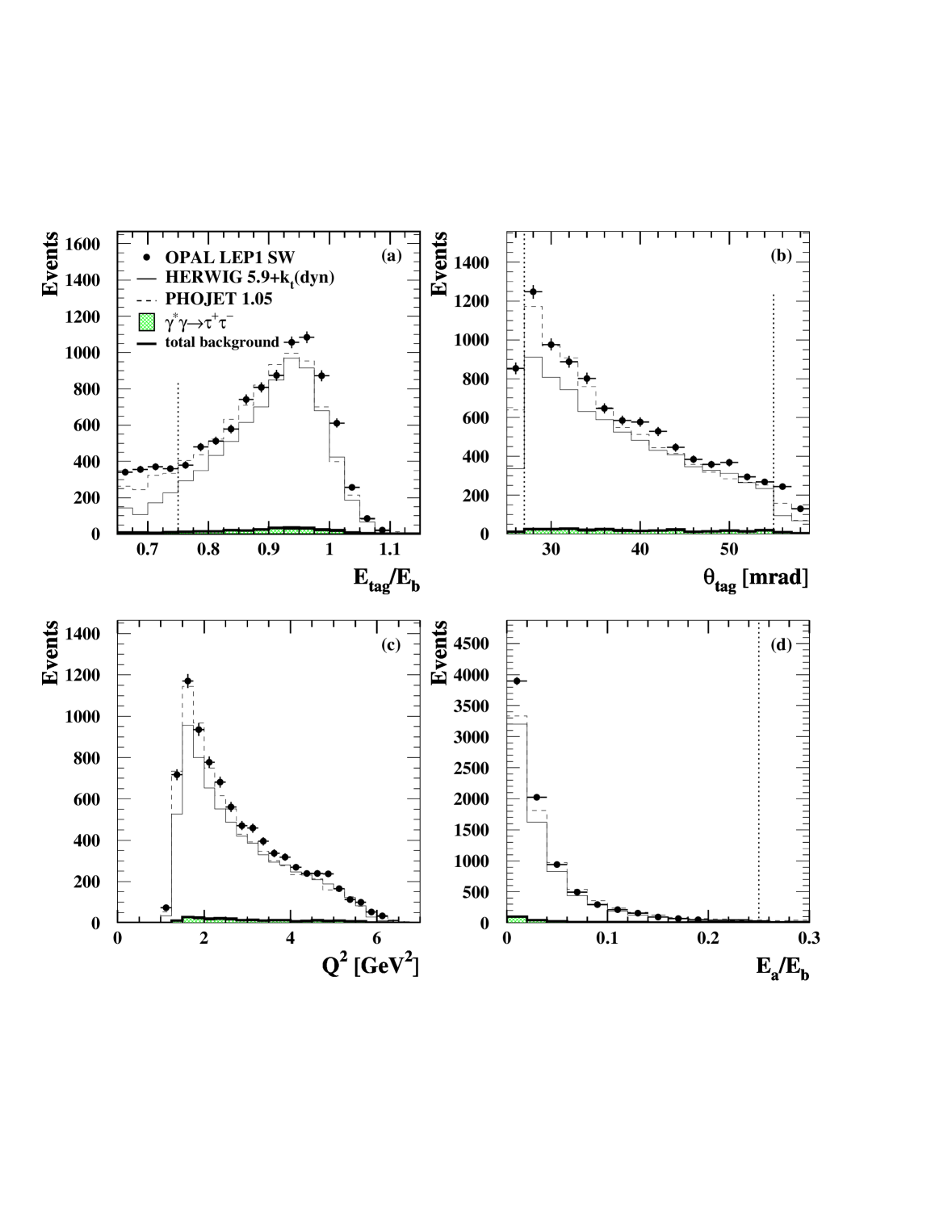
Figure 2: Comparison of data distributions with Monte Carlo predictions for the LEP1 SW sample. The dominant background source, $\gamma^{\star}\gamma\rightarrow\tau^{+}\tau^{-}$, the total background and the sum of the signal and the total background for HERWIG 5.9+$k_{\mathrm{t}}(\rm dyn)$ and PHOJET 1.05 are shown. The Monte Carlo samples have been normalised to the data luminosity. All selection cuts have been applied, except for any cut on the variable in the plot. The cuts are shown as dotted lines. The distributions shown are: a) $E_{\rm tag}$/$E_{\rm b}$, the energy of the tagged electron as a fraction of the beam energy, b) $\theta_{\rm tag}$, the polar angle of the tagged electron, c) the measured $Q^{2}$  and d) $E_{\rm a}$/$E_{\rm b}$, the energy of the most energetic electromagnetic cluster in the hemisphere opposite the tagged electron, as a fraction of the beam energy. The errors are statistical only.

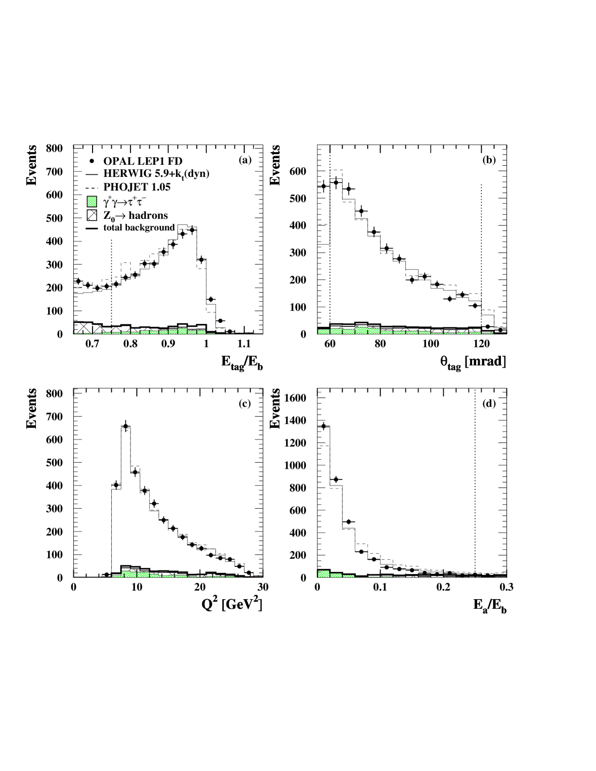
Figure 3: Comparison of data distributions with Monte Carlo predictions for the LEP1 FD sample. The dominant background sources, $\gamma^{\star}\gamma\rightarrow\tau^{+}\tau^{-}$ and $\mbox{$\rm Z^{0}$}\rightarrow$ hadrons, the total background and the sum of the signal and the total background for HERWIG 5.9+$k_{\mathrm{t}}(\rm dyn)$ and PHOJET 1.05 are shown. The Monte Carlo samples have been normalised to the data luminosity. All selection cuts have been applied, except for any cut on the variable in the plot. The cuts are shown as dotted lines. The variables in the plots are as defined in Figure 2. The errors are statistical only.

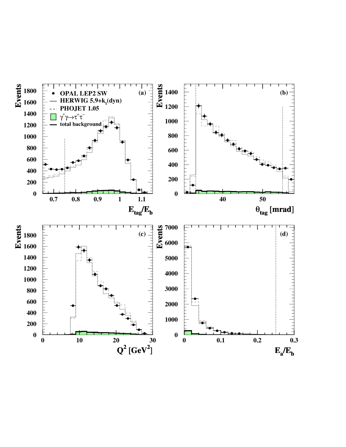
Figure 4: Comparison of data distributions with Monte Carlo predictions for the LEP2 SW sample. The dominant background source, $\gamma^{\star}\gamma\rightarrow\tau^{+}\tau^{-}$, the total background and the sum of the signal and the total background for HERWIG 5.9+$k_{\mathrm{t}}(\rm dyn)$ and PHOJET 1.05 are shown. The Monte Carlo samples have been normalised to the data luminosity. All selection cuts have been applied, except for any cut on the variable in the plot. The cuts are shown as dotted lines. The variables in the plots are as defined in Figure 2. The errors are statistical only.

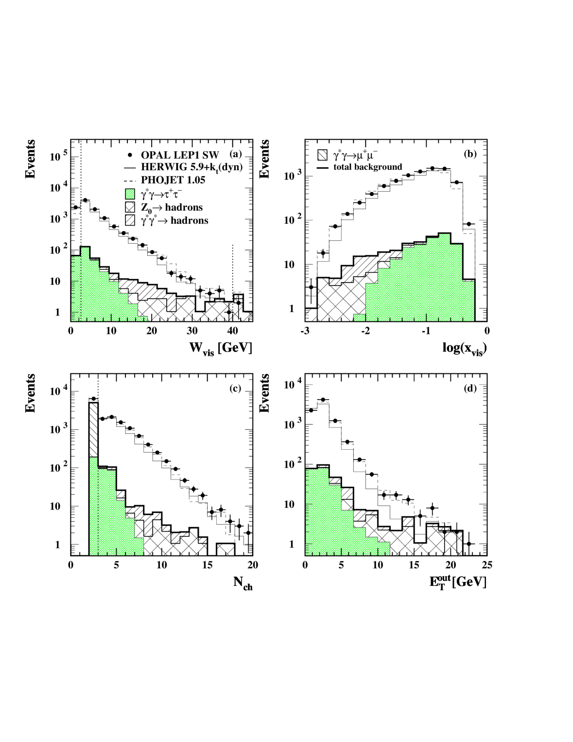
Figure 5: Comparison of data distributions with Monte Carlo predictions for the LEP1 SW sample. The dominant background sources, $\gamma^{\star}\gamma\rightarrow\tau^{+}\tau^{-}$, $\mbox{$\rm Z^{0}$}\rightarrow$ hadrons and $\mbox{$\gamma^{\star}\gamma^{\star}$}\rightarrow$ hadrons (with $P^{2}$$>$1.0 $\rm GeV^{2}$), the total background and the sum of the signal and the total background for HERWIG 5.9+$k_{\mathrm{t}}(\rm dyn)$ and PHOJET 1.05 are shown. For illustration, the background from $\gamma^{\star}\gamma\rightarrow\mu^{+}\mu^{-}$ is also shown, though it is only significant below the $N_{\rm ch}$ cut. The Monte Carlo samples have been normalised to the data luminosity. All selection cuts have been applied, except for any cut on the variable in the plot. The cuts are shown as dotted lines. The distributions shown are: a) $W_{\rm vis}$, the measured invariant mass of the hadronic final state, b) $\log{(\mbox{$x_{\rm vis}$})}$, the logarithm of the measured value of $x$. c) $N_{\rm ch}$, the number of tracks in the event and d) $E_{\rm T}^{\rm out}$, the transverse component of energy out of the tag plane. The errors are statistical only.

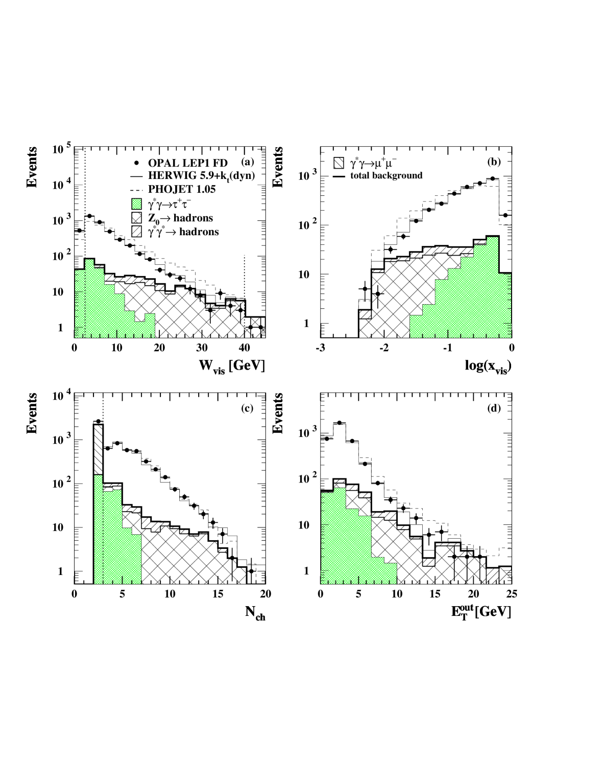
Figure 6: Comparison of data distributions with Monte Carlo predictions for the LEP1 FD sample. The dominant background sources, $\gamma^{\star}\gamma\rightarrow\tau^{+}\tau^{-}$, $\mbox{$\rm Z^{0}$}\rightarrow$ hadrons and $\mbox{$\gamma^{\star}\gamma^{\star}$}\rightarrow$ hadrons (with $P^{2}$$>$1.0 $\rm GeV^{2}$), the total background and the sum of the signal and the total background for HERWIG 5.9+$k_{\mathrm{t}}(\rm dyn)$ and PHOJET 1.05 are shown. For illustration, the background from $\gamma^{\star}\gamma\rightarrow\mu^{+}\mu^{-}$ is also shown, though it is only significant below the $N_{\rm ch}$ cut. The Monte Carlo samples have been normalised to the data luminosity. All selection cuts have been applied, except for any cut on the variable in the plot. The cuts are shown as dotted lines. The variables in the plots are as defined in Figure 5. The errors are statistical only.

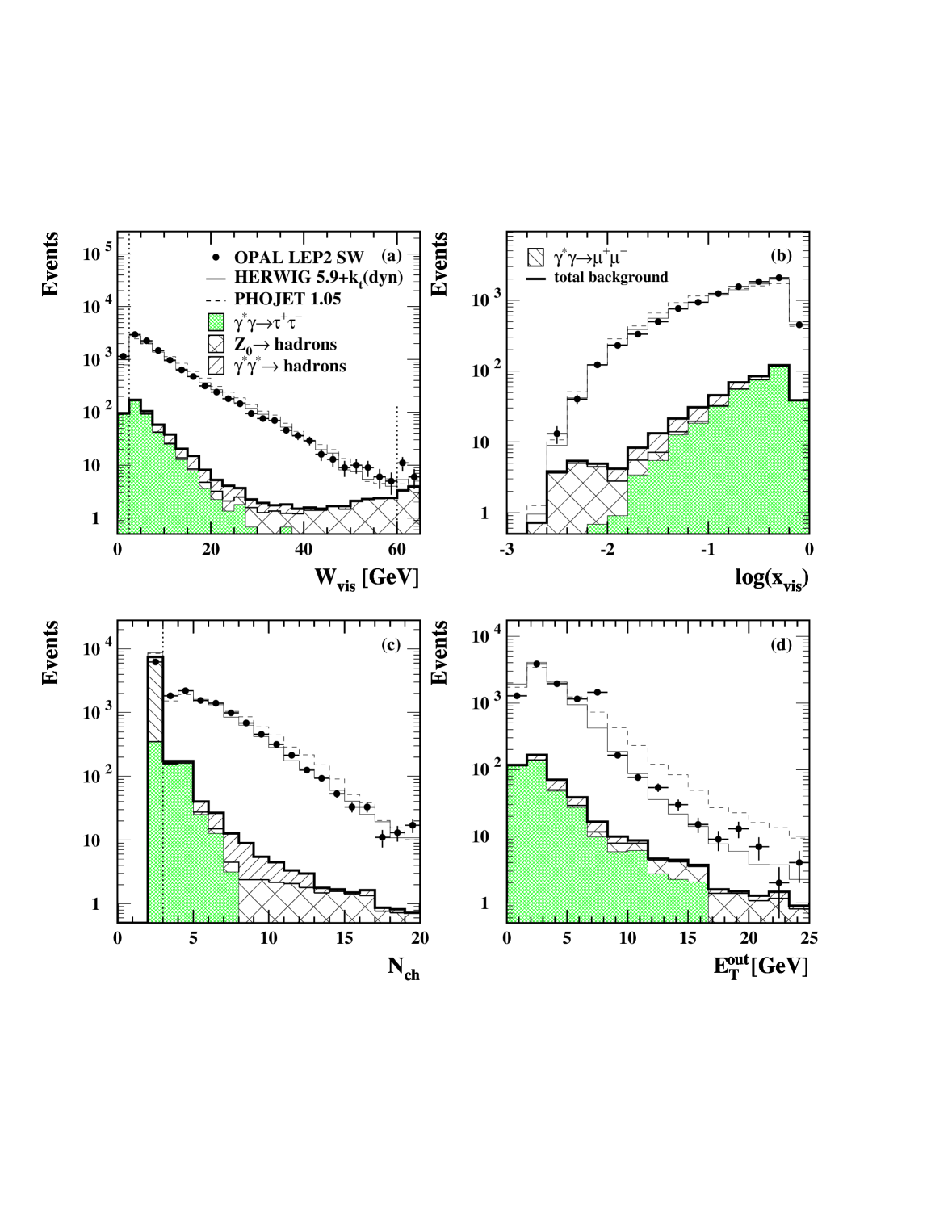
Figure 7: Comparison of data distributions with Monte Carlo predictions for the LEP2 SW sample. The dominant background sources, $\gamma^{\star}\gamma\rightarrow\tau^{+}\tau^{-}$, $\mbox{$\rm Z^{0}$}\rightarrow$ hadrons and $\mbox{$\gamma^{\star}\gamma^{\star}$}\rightarrow$ hadrons (with $P^{2}$$>$4.5 $\rm GeV^{2}$), the total background and the sum of the signal and the total background for HERWIG 5.9+$k_{\mathrm{t}}(\rm dyn)$ and PHOJET 1.05 are shown. For illustration, the background from $\gamma^{\star}\gamma\rightarrow\mu^{+}\mu^{-}$ is also shown, though it is only significant below the $N_{\rm ch}$ cut. The Monte Carlo samples have been normalised to the data luminosity. All selection cuts have been applied, except for any cut on the variable in the plot. The cuts are shown as dotted lines. The variables in the plots are as defined in Figure 5. The errors are statistical only.

The cuts applied to each sample are listed in Table 1 and shown as dotted lines in Figures 2–7. The numbers of events in each sample passing the cuts, the integrated luminosities and the $Q^{2}$ ranges are listed in Table 2. The luminosity for the LEP1 data is lower for the SW sample than for the FD sample because the SW sample does not include data from 1995.

cut	LEP1 SW	LEP1 FD	LEP2 SW
$E_{\rm tag}$/$E_{\rm b}$ min	0.75		0.775
$\theta_{\rm tag}$ min [mrad]	27	60	33.25
$\theta_{\rm tag}$ max [mrad]	55	120	55
$E_{\rm a}$/$E_{\rm b}$ max	0.25
$N_{\rm ch}$ min	3 (2 non-electron tracks)
$W_{\rm vis}$ min [$\rm GeV$]	2.5
$W_{\rm vis}$ max [$\rm GeV$]	40		60

Table 1: The selection cuts applied to each data sample.

$\langle\mbox{$Q^{2}$}\rangle$ [$\rm GeV^{2}$]	sample	luminosity [$\mbox{pb}^{-1}$]	events	$Q^{2}$ range [$\rm GeV^{2}$]
1.9	LEP1 SW	74.6	4356	1.5–2.5
3.7			4010	2.5–6.0
8.9	LEP1 FD	97.8	1909	6.0–12.0
17.5			1578	12.0–30.0
10.7	LEP2 SW	222.9	4593	7.0–13.0
17.8			5495	13.0–30.0

Table 2: The integrated luminosity, number of selected events, and $Q^{2}$ range for each data sample. The error on the luminosity is negligible.

4 Monte Carlo and background

Monte Carlo programs are used to simulate $\gamma^{\star}\gamma$ events and to provide background estimates. All Monte Carlo events are passed through the OPAL detector simulation [23] and the same reconstruction and analysis chain as real events.

It has been seen in previous studies [16, 19, 18] that Monte Carlo modelling of the hadronic final state is a large source of systematic error in the $F_{2}^{\gamma}$ measurement. While there is still no $\gamma^{\star}\gamma$ Monte Carlo generator which describes all the features of the observed hadronic final state, improved Monte Carlo programs have become available since the previous OPAL measurements of $F_{2}^{\gamma}$ and it is now possible to reject some of the models which do not describe the data adequately.

The Monte Carlo generators used to simulate signal events are HERWIG 5.9 [24], HERWIG 5.9+$k_{\mathrm{t}}(\rm dyn)$ [25], PHOJET 1.05 [26], and F2GEN [27]. HERWIG 5.9 is a general purpose Monte Carlo program which includes deep inelastic electron-photon scattering. The HERWIG 5.9+$k_{\mathrm{t}}(\rm dyn)$ version uses a modified transverse momentum distribution, $k_{t}$, for the quarks inside the photon, with the upper limit dynamically (dyn) adjusted according to the hardest scale in the event, which is of order $Q^{2}$. The distribution was originally tuned for photoproduction events at HERA [28]. PHOJET 1.05 simulates hard interactions through perturbative QCD and soft interactions through Regge phenomenology and thus is expected to provide a more complete picture of $\gamma^{\star}\gamma$ collisions than HERWIG 5.9. It is used here for the first time in an OPAL $F_{2}^{\gamma}$ analysis. In F2GEN, $\gamma^{\star}\gamma$ events are generated with a pure $\rm q\overline{q}$ final state. No QCD effects between the two quarks are simulated, and the pointlike mode was used, in which the angular distribution of the $\rm q\overline{q}$ final state is taken to be the same as for a lepton pair. The generated luminosities of the Monte Carlo samples were 3–6 times the data luminosity.

A sample was generated with each of the Monte Carlo models using the GRV LO [6] parameterisation of $F_{2}^{\gamma}$, taken from the PDFLIB library [29], as the input structure function. This version assumes massless charm quarks. To study the effect of a different input structure function on the final state, another sample was generated using HERWIG 5.9 with the SaS1D [7] parameterisation of $F_{2}^{\gamma}$.

All of the Monte Carlo programs except PHOJET 1.05 allow generation of events and cross-section calculation according to a chosen structure function. PHOJET 1.05 uses an input structure function for the total cross-section calculation but always produces the same $x$ and $Q^{2}$ distributions. The measurement of $F_{2}^{\gamma}$ requires knowledge of the structure function used to generate these distributions, so the effective internal structure function in PHOJET 1.05 was found by comparing the generator level distributions to those of HERWIG 5.9+$k_{\mathrm{t}}(\rm dyn)$ with the GRV LO structure function. The ratio of the $x$ distributions in the two samples for each $Q^{2}$ range was fitted to a polynomial, which, after multiplying by the GRV LO structure function, gave the structure function for the PHOJET 1.05 sample.

The dominant background comes from the reaction $\mbox{$\rm e^{+}e^{-}$}\rightarrow\mbox{$\rm e^{+}e^{-}$}\mbox{$\gamma^{\star}\gamma$}\rightarrow\mbox{$\rm e^{+}e^{-}$}\mbox{$\rm\tau^{+}\tau^{-}$}$ proceeding via the multiperipheral process shown in Figure 1, with $\mbox{$\rm e^{+}e^{-}$}\rightarrow\mbox{$\rm e^{+}e^{-}$}\mbox{$\gamma^{\star}\gamma$}\rightarrow\mbox{$\rm e^{+}e^{-}$}\mbox{$\rm e^{+}e^{-}$}$ giving a smaller contribution. These were simulated using the Vermaseren program [30]. The process $\mbox{$\rm Z^{0}$}\rightarrow$ hadrons also contributes significantly at LEP1 and was simulated using JETSET [31]. Because the aim is to measure the structure function of the quasi-real photon, the hadronic $\gamma^{\star}\gamma^{\star}$ events are also treated as background. They were generated using PHOJET 1.05 with the virtuality of the target photon restricted to $\mbox{$P^{2}$}>$1.0 $\rm GeV^{2}$ (LEP1) or 4.5 $\rm GeV^{2}$ (LEP2). Other sources of background considered were $\mbox{$\rm Z^{0}$}\rightarrow\tau^{+}\tau^{-}$, simulated with KORALZ [32], non-multiperipheral four-fermion events with $\rm e^{+}e^{-}$$\rm\tau^{+}\tau^{-}$ and $\rm e^{+}e^{-}$$\rm q\overline{q}$ final states, which were simulated with FERMISV [33], and $\mbox{$\rm W^{+}W^{-}$}\rightarrow$ hadrons and untagged $\gamma\gamma$ events, which were both simulated with PYTHIA [34]. The contributions from all these were found to be negligible in all the samples. The number of expected signal and background events for each data sample is shown in Table 3.

$\langle\mbox{$Q^{2}$}\rangle$ [$\rm GeV^{2}$]	signal	$\gamma^{\star}\gamma\rightarrow\tau^{+}\tau^{-}$	$\gamma^{\star}\gamma\rightarrow\mbox{$\rm e^{+}e^{-}$}$	$\mbox{$\rm Z^{0}$}\rightarrow$ had.	$\mbox{$\gamma^{\star}\gamma^{\star}$}\rightarrow$ had.
1.9	4237$\pm$66	85$\pm$6	7$\pm$1	10$\pm$2	18$\pm$3
3.7	3834$\pm$64	115$\pm$7	9$\pm$1	18$\pm$3	33$\pm$4
8.9	1749$\pm$45	85$\pm$6	3$\pm$1	42$\pm$6	30$\pm$4
17.5	1378$\pm$41	71$\pm$6	4$\pm$1	84$\pm$8	42$\pm$5
10.7	4403$\pm$68	135$\pm$6	4$\pm$1	9$\pm$1	25$\pm$2
17.8	5171$\pm$74	220$\pm$7	6$\pm$1	14$\pm$1	45$\pm$2

Table 3: The measured number of signal events (observed events corrected for background) in each data sample, and the expected number of background events according to Monte Carlo. Statistical errors only are given.

Figures 2, 3 and 4 show comparisons between data and Monte Carlo distributions for variables relating to the scattered electrons. The main differences are in the LEP1 SW data sample, where the observed cross-section for selected events is significantly higher than either of the Monte Carlo predictions. The LEP1 SW data sample is more peaked than the HERWIG 5.9+$k_{\mathrm{t}}(\rm dyn)$ prediction at low $\theta_{\rm tag}$, and there are large discrepancies between the LEP1 SW data sample and the Monte Carlo samples in the distribution of $\mbox{$E_{\rm a}$}/\mbox{$E_{\rm b}$}$ (Figure 2d), with the data having an excess at the low end of the plot. However, in this region, the anti-tag distribution is more influenced by the hadronic final state than by the anti-tagged electrons, which are almost all above the cut.

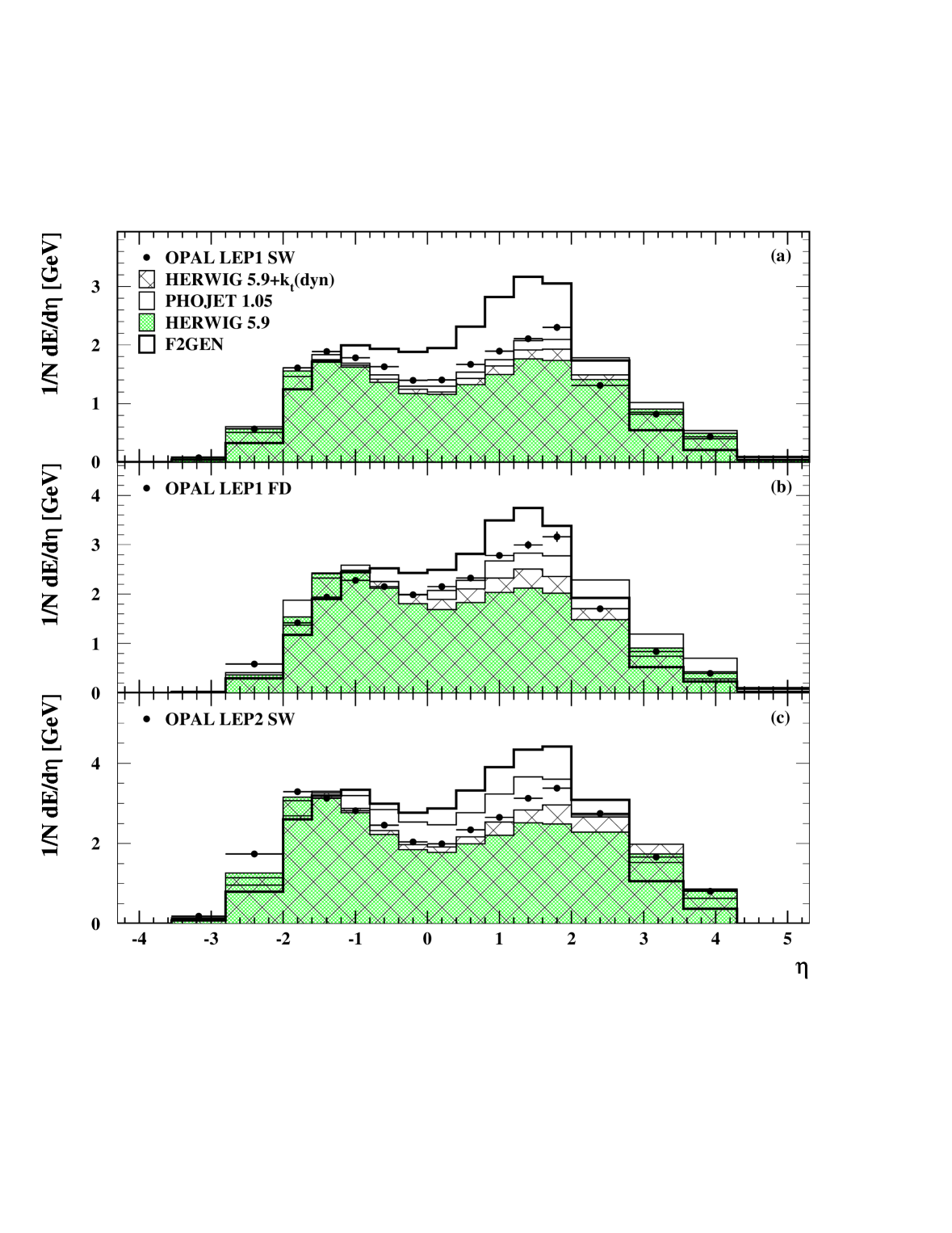
Figure 8: Comparison of hadronic energy flow per event for data and Monte Carlo as a function of the pseudorapidity, $\eta=-\log(\tan(\theta/2))$, where the polar angle $\theta$ is measured with respect to the beam axis on the side of the tagged electron. All three samples, LEP1 SW, LEP1 FD and LEP2 SW are shown. The tagged electron is not included in these plots. The errors are statistical only.

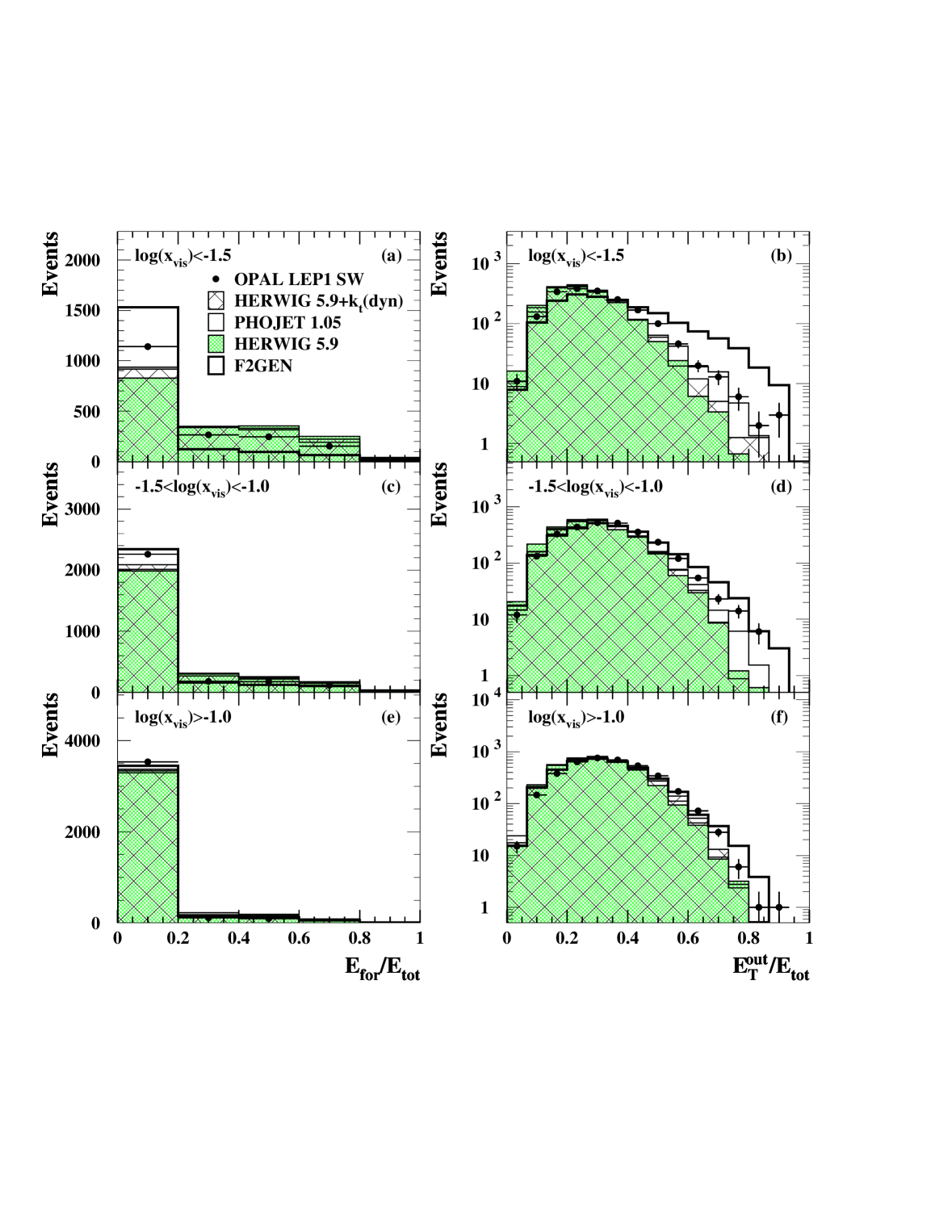
Figure 9: Data and signal Monte Carlo distributions for two alternative variables for two dimensional unfolding, for the LEP1 SW sample divided into three bins of $x_{\rm vis}$. Plots a) c) and e) show $E_{\rm for}/E_{\rm tot}$, the observed energy in the forward region divided by the total observed energy. Plots b) d) and f) show $E_{\rm T}^{\rm out}/E_{\rm tot}$, defined as the transverse component of hadronic energy out of the plane of the tagged electron, divided by the total energy. The Monte Carlo samples have been normalised to the number of data events in each plot. The errors are statistical only.

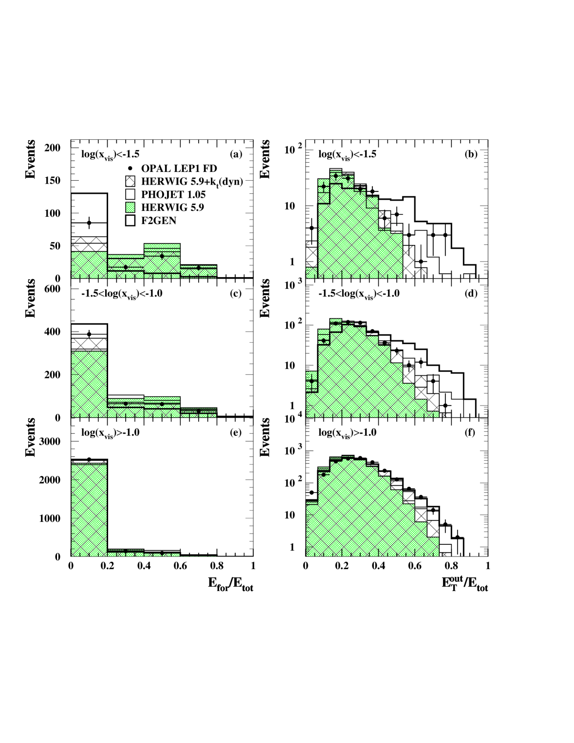
Figure 10: Data and signal Monte Carlo distributions for two alternative variables for two dimensional unfolding, for the LEP1 FD sample divided into three bins of $x_{\rm vis}$. The variables are as defined in Figure 9. The Monte Carlo samples have been normalised to the number of data events in each plot. The errors are statistical only.

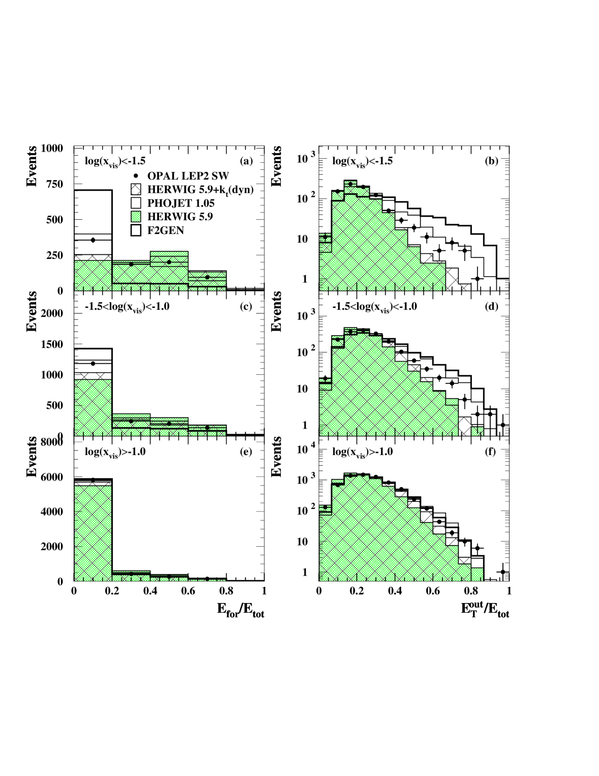
Figure 11: Data and signal Monte Carlo distributions for two alternative variables for two dimensional unfolding, for the LEP2 SW sample divided into three bins of $x_{\rm vis}$. The variables are as defined in Figure 9. The Monte Carlo samples have been normalised to the number of data events in each plot. The errors are statistical only.

In the distributions of variables related to the hadronic final state (Figures 5–11), there are large discrepancies. Figure 8 shows the hadronic energy flow as a function of pseudorapidity. It can be seen that HERWIG 5.9 tends to put too little energy in the central region of the detector, while F2GEN has a much higher peak in the central region than the data. PHOJET 1.05 gives the best description of the data in these plots.

The large differences between HERWIG 5.9+$k_{\mathrm{t}}(\rm dyn)$ and PHOJET 1.05 in the $W_{\rm vis}$ distributions (Figures 5a, 6a and 7a) and the $x_{\rm vis}$ distributions (Figures 5b, 6b and 7b) are mostly due to the fact that PHOJET 1.05 does not use the input structure function to generate the $x$ distribution, although there are also differences arising from the final state modelling. The quantity $x_{\rm vis}$ is calculated by inserting $W_{\rm vis}$ into equation 4. For the number of tracks, $N_{\rm ch}$, in the LEP1 SW sample (Figure 5c), the data distribution is above the Monte Carlo distributions at high $N_{\rm ch}$. The Monte Carlo descriptions of $N_{\rm ch}$ are closer to the data in the LEP1 FD and LEP2 SW samples (Figures 6c and  7c). There are significant differences in the distributions of $E_{\rm T}^{\rm out}$ (Figures 5d, 6d and 7d on a linear scale and Figures 9, 10 and 11 on a logarithmic scale and divided into three bins of $x_{\rm vis}$). $E_{\rm T}^{\rm out}$ is the transverse hadronic energy out of the plane containing the beam line and the tagged electron:

$$\mbox{$E_{\rm T}^{\rm out}$}=\sum_{i}E_{i,\rm t}|\sin\phi_{i}|$$ (5)

where $i$ runs over all particles in the hadronic final state, with transverse energy $E_{i,\rm t}$. The azimuthal angle $\phi_{i}$ is measured from the tagged electron. HERWIG 5.9 has too few events at large $E_{\rm T}^{\rm out}$ and F2GEN has too many, especially at low values of $x_{\rm vis}$. Also shown in Figures 9, 10 and 11 is $E_{\rm for}/E_{\rm tot}$, the observed energy in the forward region divided by the total observed energy. Of the four Monte Carlo models, PHOJET 1.05 shows the best agreement with the data in the hadronic final state, HERWIG 5.9+$k_{\mathrm{t}}(\rm dyn)$ describes the data better than HERWIG 5.9, and F2GEN gives the worst description of the data. For the final results, only PHOJET 1.05 and HERWIG 5.9+$k_{\mathrm{t}}(\rm dyn)$ are used; however, all four Monte Carlo models are used in studies of the unfolding methods.

None of the Monte Carlo programs discussed above contain radiative corrections to the deep inelastic scattering process. These are dominated by initial state radiation from the deeply inelastically scattered electron. The final state radiation is experimentally integrated out due to the finite granularity of the calorimeters. The Compton scattering process contributes very little, and the radiative corrections due to radiation of photons from the electron that produced the quasi-real target photon were shown to be very small [35].

In this analysis the radiative corrections have been evaluated using the RADEG program [36], which includes initial state radiation and the Compton scattering process. The calculations are performed using mixed variables, which means that $Q^{2}$ is calculated from electron variables, while $W^{2}$ is calculated from hadronic variables. The value of $x$ is found from $W^{2}$ and $Q^{2}$, exactly as for the experimental analysis. The RADEG program allows calculation of differential cross-sections in bins of $x$ and $Q^{2}$, with or without radiative corrections, while applying the experimental restrictions on the electron energy and polar angle, the minimum invariant mass and the anti-tag angle. The predicted ratio of the differential cross-section for each bin of the analysis is used to correct the data, i.e. the measured $F_{2}^{\gamma}$ is multiplied by the ratio of the non-radiative and the radiative cross-sections. The radiative corrections reduce the cross-section in the phase space of the present analysis. They are largest at low values of $x$. The size of the largest correction to any bin is 14$\%$. The radiative corrections are insensitive to the choice of $F_{2}^{\gamma}$ in the calculation, for example, the difference between the predicted corrections for the GRV and the QPM structure functions is negligible in all regions of $x$ and $Q^{2}$.

Several theoretical ansatzes exist for how $F_{2}^{\gamma}$ should behave as a function of $P^{2}$ [37, 38, 39]. They all predict a decrease of $\mbox{$F_{2}^{\gamma}$}(x,\mbox{$Q^{2}$},\mbox{$P^{2}$}\neq 0)$ with $P^{2}$ which is strongest at low values of $x$. This means that applying a correction to obtain an $F_{2}^{\gamma}$ which is valid at $\mbox{$P^{2}$}=0$ would change the shape of the measured $F_{2}^{\gamma}$. The size of the effect was studied based on the GRS [37] and SaS1D [38] parameterisations using three values of $P^{2}$: $0.01,0.02$ and $0.03$ $\rm GeV^{2}$, and four values of $Q^{2}$: $1.9,3.7,9.5$ and $17.6$ $\rm GeV^{2}$. These values reflect the range of $\langle\mbox{$P^{2}$}\rangle$ values expected in the data, and the $\langle\mbox{$Q^{2}$}\rangle$ values of the data samples. The largest suppression observed at $x=0.003$ for $\mbox{$P^{2}$}=0.01/0.02/0.03$ $\rm GeV^{2}$ is around $7/12/17\%$; however, at low $x$ the predictions differ by more than a factor of two. Because the distribution of $P^{2}$ in the data is not known and the theoretical predictions differ significantly, no correction is applied.

5 Determination of $F_{2}^{\gamma}$

5.1 Unfolding

Unfolding is a statistical technique which is used in this analysis to correct the measured distributions for detector effects. The unfolding problem can be described as follows: A measurement $g_{j}$ is made of a true distribution $f_{i}$, with $j$ and $i$ bins respectively. The $g_{j}$ distribution differs from $f_{i}$ because of

• Limited resolution:
  Events in a certain bin of the true distribution can be spread into several bins in the measured distribution. In $\gamma^{\star}\gamma$ events this can be due to missing energy in the forward region (FD and SW plus the beampipe), as well as the intrinsic energy resolution of the subdetectors.

• Limited acceptance:
  Some events fail the cuts and therefore contribute only to the true $x$ distribution, and not to the measured distribution.

• Background:
  There are also events originating from other reactions which only contribute to the measured distribution.

Resolution and acceptance effects can be described in terms of a response matrix $A_{ij}$. The distributions $g_{j}$ and $f_{i}$ are then related by

$$g_{j}=\sum_{i=1}^{n}A_{ij}f_{i}+b_{j}$$ (6)

where $b_{j}$ is the background distribution. Equation 6 cannot simply be inverted to find $f_{i}$ because this does not lead to a stable solution. Instead, after $b_{j}$ is subtracted, $f_{i}$ is estimated from a procedure which includes a smoothing (or regularisation) of the distribution to reduce statistical fluctuations. The response matrix $A_{ij}$ is found from Monte Carlo simulation. After unfolding, $F_{2}^{\gamma}$ is determined by reweighting the input structure function of the Monte Carlo according to the ratio of the unfolded $x$ distribution to the $x$ distribution in the Monte Carlo:

$$\mbox{$F_{2,i}^{\gamma}$}=\frac{\langle f(x)\thinspace\mbox{$F_{2,\rm MC}^{\gamma}$}(x)\rangle_{i}}{N_{{\rm MC},i}}$$ (7)

where $F_{2,\rm MC}^{\gamma}$ is the input structure function of the Monte Carlo sample used for unfolding, $N_{{\rm MC},i}$ is the number of events in the Monte Carlo sample in the $i$th bin and $f(x)$ is the unfolded $x$ distribution, obtained from a quadratic spline fit to $f_{i}$, with $f(x)=0$ at the edges of the acceptance region. $F_{2,i}^{\gamma}$ represents the measured value of the average $F_{2}^{\gamma}$ of the events in bin $i$ of the unfolded distribution, and not the average over $x$. The distinction is important mainly at low $x$, where $f(x)$ changes most rapidly.

The main unfolding program used for this analysis was GURU [40]; the programs RUN [41] and BAYES [42] were used to check the unfolding. In previous OPAL $F_{2}^{\gamma}$ analyses, only RUN was used. The programs GURU and RUN are similar in principle, but have different implementations. Due to its use of standard matrix techniques, GURU has a much simpler structure and is easier to modify than RUN, which uses a maximum likelihood fit with spline functions. The BAYES program performs unfolding using an iterative method based on Bayes’ theorem, leaving regularisation to the user (e.g. a polynomial fit after each iteration except the last). The programs GURU, RUN and BAYES were compared by unfolding test distributions including experimental data. The result of one such study, unfolding the LEP1 SW data with HERWIG 5.9+$k_{\mathrm{t}}(\rm dyn)$, using the measured distribution $x_{\rm vis}$, is shown in Figure 12a. The results from the three programs are generally consistent, though the BAYES program tends to assign smaller errors than the other two.

The amount of regularisation in the unfolding is set by the number of degrees of freedom (NDF). It can be seen in Figure 12b that increasing this number leads to larger unfolding errors. Reducing the number of degrees of freedom increases the correlations between the bins. The number of degrees of freedom to be used is determined by the GURU program from statistical analysis of the data distributions, as described in the GURU documentation [40].

The unfolding of the variable $x$ is done on a logarithmic scale in order to study the low-$x$ region in more detail. Several improvements to the unfolding procedure used in previous OPAL analyses have been implemented. These are described in the following sections.

5.2 Reconstruction of $\boldmath W$

The visible hadronic mass squared is defined by

$$\mbox{$W_{\rm vis}^{2}$}=(\sum_{i}E_{i})^{2}-(\sum_{i}p_{i,x})^{2}-(\sum_{i}p_{i,y})^{2}-(\sum_{i}p_{i,z})^{2}$$ (8)

where $i$ runs over all tracks and clusters in the hadronic final state, with energy $E_{i}$ and momentum vector $(p_{i,x},p_{i,y},p_{i,z})$. Because hadronic showers are not well contained in the electromagnetic calorimeters, and some energy is lost in the beampipe, the measured energy in the forward region is less than the true energy. It is possible to improve the reconstruction of $W_{\rm vis}$ by including kinematic information from the tagged electron [43]. $W_{\rm vis}^{2}$ can also be written as

$$\mbox{$W_{\rm vis}^{2}$}=(\sum_{i}p_{i+})(\sum_{i}p_{i-})-(\sum_{i}p_{i,\rm t})^{2}$$ (9)

where $p_{i\pm}=E_{i}\pm p_{i,z}$ and $p_{i,\rm t}=\sqrt{{p_{i,x}}^{2}+{p_{i,y}}^{2}}$. Using conservation of energy and momentum, and assuming that the untagged electron travels along the beam direction, the sums over $p_{i+}$ and $p_{i,\rm t}$ can be replaced by electron variables, leading to

$$\mbox{$W_{\rm rec}^{2}$}=(p_{\rm beam+}-p_{\rm tag+})(\sum_{i}p_{i-})-(p_{\rm tag,t})^{2}$$ (10)

where $p_{\rm beam+}$ and $p_{\rm tag+}$ are calculated for the tagged electron before and after scattering, respectively, and $p_{\rm tag,t}$ is calculated according to the definition of $p_{i,\rm t}$, above, for the tagged electron. When using Equation 10 instead of Equation 9 to evaluate the measured hadronic mass of each event, the hadronic energy enters only through the $p_{i-}$ term. This is an advantage because the leptonic energy resolution is usually better than the hadronic energy resolution. The (reconstructed) variable formed in this way is called $W_{\rm rec}$. The corresponding measurement of $x$ is called $x_{\rm rec}$. The improvement in the resolution when using $W_{\rm rec}$ instead of $W_{\rm vis}$ depends on how well the hadronic system is measured, and is therefore both detector dependent and model dependent.

Even after the above technique has been applied, the value of $W_{\rm rec}$ is still generally smaller than the true value. This is mainly due to energy losses in the forward calorimeters, in which only about 40% of the hadronic energy is observed. This makes the measurement very dependent on the angular distribution of the hadrons in the final state. In an attempt to make the energy response of the detector more uniform and to reduce the systematic error due to the uncertainty in the Monte Carlo modelling, a new (corrected) variable is formed: $W_{\rm cor}$, along with the corresponding $x$ measurement $x_{\rm cor}$, in which the contribution from the forward region has been scaled by a factor of 2.5. This factor was obtained by comparing the generated and measured energy in the forward region in Monte Carlo events. The uncertainty of this factor has been taken into account in the evaluation of the systematic errors.

$$W_{\rm cor}^{2} = (p_{\rm beam+}-p_{\rm tag+})(\sum_{i}p^{\prime}_{i-})-(p_{\rm tag,t})^{2}$$ (11)

$$p^{\prime}_{i-} = \left\{\begin{array}[]{ll}2.5p_{i-}&\mbox{ for clusters observed in SW or FD}\\ p_{i-}&\mbox{ otherwise}\\ \end{array}\right.$$ (14)

Figure 13a shows the correlation between the generated $W$ and the three measured quantities $W_{\rm vis}$, $W_{\rm rec}$ and $W_{\rm cor}$ for the LEP2 SW sample generated with HERWIG 5.9+$k_{\mathrm{t}}(\rm dyn)$. The spread of $W_{\rm cor}$ in $W$ is larger than that of the other two variables, because in $W_{\rm cor}$ more weight is given to the forward region, where the energy resolution is worse than in the central region. In general, $W_{\rm cor}$ is still lower than $W$, mainly because of energy lost in the beampipe. Figure 13b shows the correlation between the generated energy in the forward region and the scaled observed energy in that region, $E_{\rm cor}$.

The three measured variables $x_{\rm vis}$, $x_{\rm rec}$ and $x_{\rm cor}$ can be used to unfold the true variable $x$. The difference between the results is model dependent and generally small when using Monte Carlo models that already give a good description of the hadronic final state (Figure 12c).

5.3 Two dimensional unfolding

The GURU program can also be used to perform unfolding in two dimensions. As with the attempts to improve the $W$ reconstruction described above, the motivation is to reduce the dependence of the unfolding on a particular Monte Carlo model. There is information in every event about the angular distribution of energy in the detector, but it is not fully exploited if only $x$ is used in the unfolding procedure. Including another variable in a second unfolding dimension makes more direct use of this information.

Two variables were considered as possible second unfolding variables. They were chosen because they are very sensitive to the angular distribution of the hadrons in the final state:

• $E_{\rm T}^{\rm out}/E_{\rm tot}$, the transverse hadronic energy out of the plane containing the beam line and the tagged electron (see Equation 5), divided by the total observed energy.

• $E_{\rm for}/E_{\rm tot}$, the observed energy in the forward calorimeters divided by the total observed energy.

These variables are shown in Figures 9–11. To test the two dimensional unfolding procedure, a random number was used as the second variable. The results are shown in Figure 12d. They are consistent with one dimensional unfolding, which is as expected since there is no extra information in a random number.

5.4 Testing the unfolding methods

To find which of the unfolding methods was the most reliable, OPAL data was unfolded with four Monte Carlo programs HERWIG 5.9, HERWIG 5.9+$k_{\mathrm{t}}(\rm dyn)$  PHOJET 1.05 and F2GEN. Despite not giving good descriptions of the data, HERWIG 5.9 and F2GEN were included in this study to investigate the effectiveness of the new techniques using extreme models. The best methods are considered to be those which give the smallest difference between the unfolded results with the four Monte Carlo models. The quantity compared is ${\chi^{2}}$, defined by

$$\mbox{${\chi^{2}}$}=\frac{1}{4}\sum_{\rm models}\sum_{i}\left(\frac{\mbox{$F_{2}^{\gamma}$}_{i}-\langle\mbox{$F_{2}^{\gamma}$}_{i}\rangle}{\sigma_{i}}\right)^{2}$$ (15)

where $\mbox{$F_{2}^{\gamma}$}_{i}$ is the value of the unfolded result in the $i$th bin, $\langle\mbox{$F_{2}^{\gamma}$}_{i}\rangle$ is the average of the results from all four Monte Carlo models and $\sigma_{i}$ is the statistical error for $\mbox{$F_{2}^{\gamma}$}_{i}$. The values of ${\chi^{2}}$ are shown in Table 4 and the results of the unfolding are shown in Figures 14–16. The ${\chi^{2}}$ values show how large the differences between the models are, compared to the statistical error. In general, the lowest values of ${\chi^{2}}$ were obtained using two-dimensional unfolding with $x_{\rm cor}$ as the first variable and $E_{\rm T}^{\rm out}/E_{\rm tot}$ as the second variable, which consequently is used as the standard unfolding method for the results. The ${\chi^{2}}$ values are usually smaller for the LEP1 FD sample than the other two. This is partly due to the smaller number of bins. Additionally, the lower statistics in the LEP1 FD sample mean that any difference between the Monte Carlo programs would be less significant.

With both two dimensional unfolding and with one dimensional unfolding using $x_{\rm cor}$ as the unfolding variable, the spread between the results with the different models is reduced compared to one dimensional unfolding results using $x_{\rm vis}$, and the agreement between F2GEN and the other models is especially improved. Using different unfolding methods with the HERWIG 5.9+$k_{\mathrm{t}}(\rm dyn)$ and PHOJET 1.05 samples makes less difference than with the other two Monte Carlo samples, which is as expected for models which give a better description of the data.

As a final test of the unfolding method, several samples of Monte Carlo events generated using HERWIG 5.9 with the SaS1D structure function were unfolded using HERWIG 5.9 with the GRV LO structure function. The results are shown in Figure 17. The measured structure function agrees with the input structure function within the statistical precision of the Monte Carlo events generated using the SaS1D structure function.

The effect of taking into account the shape of $f(x)$ within each bin of $x$, as in Equation 7, compared to simply extracting $F_{2}^{\gamma}$ as the average input structure function of the Monte Carlo sample times the ratio of the number of unfolded events and the number of Monte Carlo events in each bin, was also investigated with these samples. The effect is largest in the lowest $x$ bins for LEP2 SW, where the decrease in the value of $F_{2}^{\gamma}$ when taking into account the shape within the bin is a little less than the statistical errors shown in Figure 17.

		${\chi^{2}}$
		1D		2D, $E_{\rm T}^{\rm out}/E_{\rm tot}$		2D, $E_{\rm for}/E_{\rm tot}$
$\langle\mbox{$Q^{2}$}\rangle$ [$\rm GeV^{2}$]	sample	$x_{\rm vis}$	$x_{\rm cor}$	$x_{\rm rec}$	$x_{\rm cor}$	$x_{\rm rec}$	$x_{\rm cor}$
1.9	LEP1 SW	66.8	29.1	22.1	9.6	24.7	26.9
3.7		53.1	26.1	13.5	8.1	19.5	16.8
8.9	LEP1 FD	15.4	6.8	7.1	3.4	10.7	8.7
17.5		8.5	4.5	8.8	12.4	4	4.1
10.7	LEP2 SW	62.5	22.4	18.7	6.8	20.6	16.8
17.8		57.2	18.3	13	8.4	57.7	15.4

Table 4: ${\chi^{2}}$, as defined in Equation 15, for different unfolding methods. The number of bins in $x$ was 4 for the LEP1 SW and LEP2 SW samples, and 3 for the LEP1 FD samples.

6 Results

The photon structure function $F_{2}^{\gamma}$ is measured by unfolding each data sample in bins of $\mbox{log}(x)$. Each OPAL data sample is divided into two ranges of $Q^{2}$ containing approximately equal numbers of events. The ranges correspond to $\langle\mbox{$Q^{2}$}\rangle$ values of 1.9 and 3.7 $\rm GeV^{2}$ for the LEP1 SW sample, and 8.9 (10.7) and 17.5 (17.8) $\rm GeV^{2}$ for the LEP1 FD (LEP2 SW) sample, where the average $Q^{2}$ values have been obtained from the data. $F_{2}^{\gamma}$ is unfolded to a given $\langle\mbox{$Q^{2}$}\rangle$ value and does not correspond to an average in each bin of $Q^{2}$.

The results are listed in Table 6. The quoted values were measured as the average $F_{2}^{\gamma}/\mbox{$\alpha$ }$ in each bin of $x$ weighted by the unfolded $x$ distribution, according to Equation 7, then corrected to the log centre of each bin, except for the highest $x$ bins where the log centre of that portion of the bin below the charm threshold for $m_{c}=1.5$ $\rm GeV$ was used. The bin-centre corrections are the average of the GRV LO and SaS1D predictions for the correction from the average $F_{2}^{\gamma}$ over the bin to the value of $F_{2}^{\gamma}$ at the nominal $x$ position.

The results are also corrected for radiative effects. The radiative corrections were calculated using the RADEG [36] program and are listed in Table 7, along with the bin-centre corrections. The statistical correlations between bins are shown in Table 8.

The central value of $F_{2}^{\gamma}$ in each $x$ bin is the average of the data unfolded with HERWIG 5.9+$k_{\mathrm{t}}(\rm dyn)$ and PHOJET, using two dimensional unfolding with $x_{\rm cor}$ as the first variable and $E_{\rm T}^{\rm out}/E_{\rm tot}$ as the second variable. Standard HERWIG 5.9 and F2GEN were not used as they are not in acceptable agreement with the data. The systematic errors are evaluated by repeating the unfolding with one parameter varied at a time and finding the shift in the result. The systematic errors are combined by adding all of the individual contributions in quadrature. The summing is done separately for positive and negative errors. The systematic effects considered are listed below.

• Monte Carlo modelling:
  The quoted result is the average of the results obtained using HERWIG 5.9+$k_{\mathrm{t}}(\rm dyn)$ and PHOJET 1.05. The errors are symmetrical and equal to half the difference between the results with the two Monte Carlo programs.

• Unfolding method:
  The unfolding was repeated with $E_{\rm for}/E_{\rm tot}$ as the second variable, instead of $E_{\rm T}^{\rm out}/E_{\rm tot}$.

• Unfolding parameters:
  The number of bins used for the measured variable can be different from the number of bins used for the true variable (though it should be at least as large). The standard result has 6 bins in the measured variable. This was increased to 8 to estimate the systematic effects of unfolding.

• $W$ reconstruction:
  The weighting applied to the energy in the forward calorimeters was varied between 2.0 and 3.0. This check allows for uncertainty in the treatment of forward energy.

• Variations of cuts:
  The composition of the selected events was varied by changing the cuts one at a time. The size of the variations reflect the resolution of the measured variables and are sufficiently small not to change the average $Q^{2}$ of the sample significantly, or remove too many events from any single $x$ bin. The variations of the cuts are listed in Table 5.

• Off-momentum electrons:
  There is a possible contamination of off-momentum background in one region of azimuthal angle $\phi$ in the 183 $\rm GeV$ data, so as a precaution this $\phi$ region was removed in the measurement of $F_{2}^{\gamma}$, and the difference from the result with the $\phi$ region left in was included as a systematic error.

• Calibration of the tagging detectors (FD and SW):
  The energy of the tagged electron in the Monte Carlo samples was scaled by $\pm 1\%$, to allow for uncertainty in the simulation of the detectors. The size of the variation was motivated by a comparison of the $\mbox{$E_{\rm tag}$}/\mbox{$E_{\rm b}$}$ distributions in data and Monte Carlo.

• Measurement of the hadronic energy:
  The main uncertainty is in the calibration of the electromagnetic calorimeters (excluding the forward region which is dealt with separately). This was varied by $\pm$3% in the Monte Carlo samples. The track quality criteria were also varied, but the effects were negligible.

• Simulation of background:
  The hadronic background events at LEP1 stem from the production of photons or light mesons with a large fraction of the beam energy. The mesons fake an electron tag due to their decays into photons. The cross-section for these events was measured by OPAL with an accuracy of about 50%, and found to be consistent with the JETSET prediction [44]. The normalisation of the simulated background was therefore varied by $\pm$50%.

• Bin-centre correction:
  The corrections depends on the shape of $F_{2}^{\gamma}$ in each bin. The average of the corrections based on GRV LO and SaS 1D was used, as these parameterisations are the closest to the data. The error is half the difference between the GRV LO and SaS 1D corrections, and is symmetric.

Because the estimation of each source of systematic error has some statistical fluctuation due to the changing distributions (e.g. when a cut is varied), the quadratic sum of all individual sources is an overestimate of the total systematic error. The expected statistical component of each source of systematic error that changes the data sample is determined by unfolding 8 Monte Carlo samples, each about the same size as the data sample.

The corrected systematic error on the $i$th bin from source $k$ is then

$$(\Delta^{\prime}f_{i,k})^{2} = (\Delta f_{i,k})^{2}-\sigma_{\Delta f_{i,k}}^{2}\mbox{ for }\Delta f_{i,k}^{2}>\sigma_{\Delta f_{i,k}}^{2}$$

$$\Delta^{\prime}f_{i,k} = 0\mbox{ otherwise}$$ (16)

where $\Delta f_{i,k}$ is the shift on the $i$th bin in the data when changing a parameter $k$, and $\sigma_{\Delta f_{i,k}}$ is the expected statistical component of the shift, which is approximated by the statistical spread in the systematic error estimates for source $k$ in the 8 Monte Carlo samples. In a few cases this was larger than the statistical error in the data. In these cases $\sigma_{\Delta f_{i,k}}$ was set to the statistical error in the data, in order not to hide possibly significant systematic errors. This procedure means that for the individual systematic errors either the expected statistical component is subtracted, or the error is set to zero if the observed shift in the data is consistent with a statistical fluctuation as predicted by the 8 Monte Carlo samples.

The total systematic error is the quadratic sum of all the individual contributions $\Delta^{\prime}f_{i,k}$ from the above sources. The sum is made separately for deviations above and below the standard result. The systematic errors from each source as a function of $x$ and $Q^{2}$ are listed in Table 9.

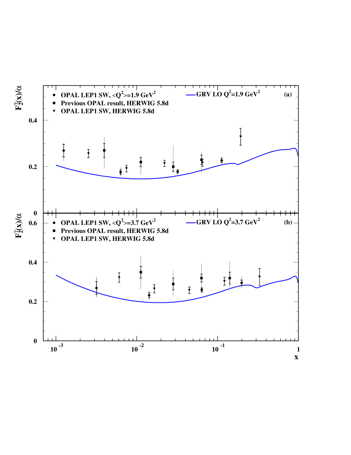
Figure 18: The measurement of $F_{2}^{\gamma}/\mbox{$\alpha$ }$ using the LEP1 SW sample, for $\langle\mbox{$Q^{2}$}\rangle$ values of (a) 1.9 and (b) 3.7 $\rm GeV^{2}$. Also shown are the previous OPAL results in these $Q^{2}$ ranges, which were unfolded using HERWIG 5.8d, and the result of unfolding the LEP1 SW data using HERWIG 5.8d. For each point, the inner error bars show the statistical error and the full error bars show the total error, except for the new result with HERWIG 5.8d, for which only statistical errors are shown. The positions of the new OPAL points are as given in Table 6. The other points are shown at the centre of the $\log(x)$ bin. The curves show the GRV LO structure function.

The results are shown along with previous OPAL measurements of $F_{2}^{\gamma}$ [16] in Figures 18 and 19. The overlapping results from the LEP1 FD and LEP2 SW samples are in good agreement. The measurements of $F_{2}^{\gamma}$ using LEP1 data for $\mbox{$\langle\mbox{$Q^{2}$}\rangle$}=1.9$ $\rm GeV^{2}$ and $\mbox{$\langle\mbox{$Q^{2}$}\rangle$}=3.8$ $\rm GeV^{2}$ are lower than the previous OPAL LEP1 results, which were unfolded using HERWIG 5.8d. Repeating the unfolding with HERWIG 5.8d gives results which are consistent with the old analysis, but with better precision. The HERWIG 5.8d Monte Carlo model has now been replaced by HERWIG 5.9+$k_{\mathrm{t}}(\rm dyn)$, which gives a better description of the data. The results in the four higher $Q^{2}$ bins are consistent with previous OPAL measurements, and have smaller errors. The previous LEP1 results with electrons tagged in SW or FD are superseded by the present analysis.

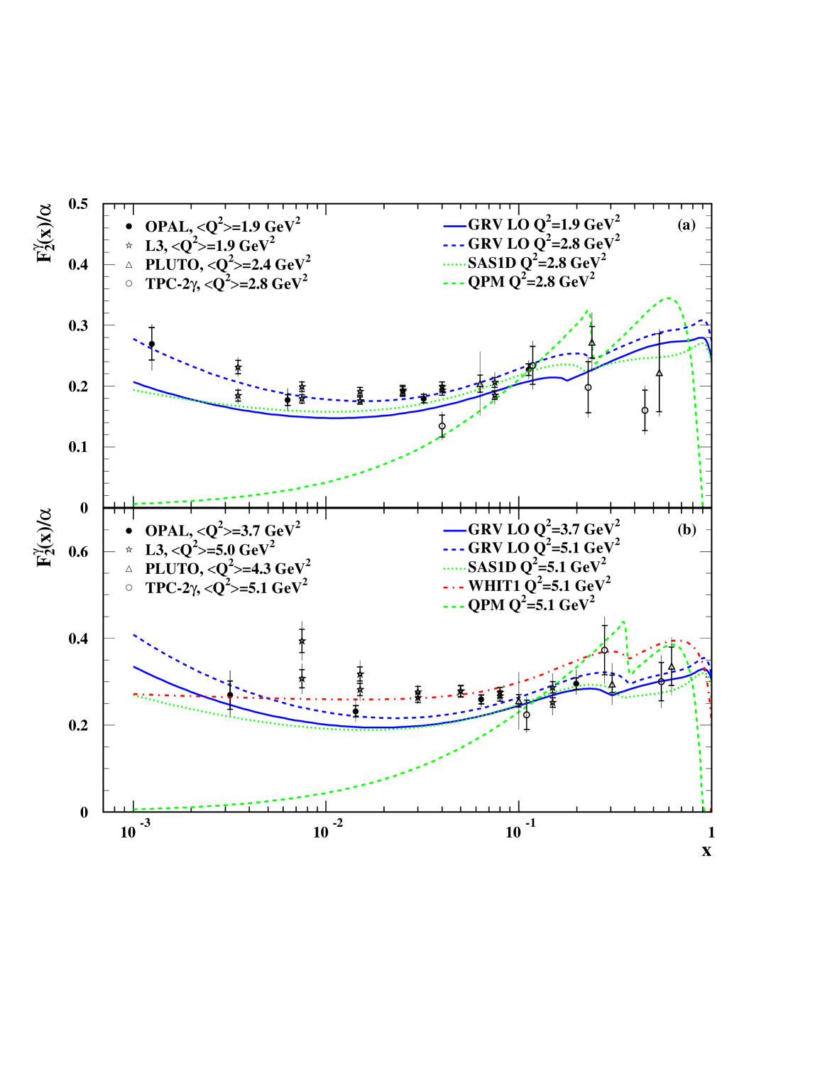
Figure 20: The measurement of $F_{2}^{\gamma}/\mbox{$\alpha$ }$ using the LEP1 SW sample, for $\langle\mbox{$Q^{2}$}\rangle$ values of (a) 1.9 and (b) 3.7 $\rm GeV^{2}$. Also shown are the results from L3 [18] PLUTO [10], and TPC/2$\gamma$ [13]. For L3 the two sets of points were unfolded using different Monte Carlo programs. The lower / upper points correspond to PHOJET 1.05 / TWOGAM. For each point, the inner error bars show the statistical error and the full error bars show the total error. The positions of the new OPAL points are as given in Table 6. The other points with closed symbols are shown at the centre of the $\log(x)$ bin, and those with open symbols are shown at the average $x$ value of the bin. The curves show the GRV LO, SaS1D, WHIT1 and QPM structure functions.

In Figures 20 and 21 the results are compared to measurements of $F_{2}^{\gamma}$ from other experiments: TPC/2$\gamma$ [13], PLUTO [10], TOPAZ [15], ALEPH [19], DELPHI [17] and L3 [18]. Also shown in Figures 20 and 21 are the GRV LO, SaS1D and WHIT1 [8] parameterisations of $F_{2}^{\gamma}$, and the naive quark-parton model (QPM). The QPM prediction, which only models the point-like component of $F_{2}^{\gamma}$, is calculated for four active flavours with masses of 0.2 $\rm GeV$ for light quarks and 1.5 $\rm GeV$ for charm quarks.

The previous results are found to be generally consistent with the new OPAL measurements. The largest differences are from the older measurement by TPC/2$\gamma$ at $\mbox{$\langle\mbox{$Q^{2}$}\rangle$}=2.8$ $\rm GeV^{2}$, which suggests a different shape of $F_{2}^{\gamma}$ to all the other measurements. The L3 results obtained at $\mbox{$\langle\mbox{$Q^{2}$}\rangle$}=5.0$ $\rm GeV^{2}$ are consistently higher than the OPAL measurements. However, because the L3 points are highly correlated, due to the finer binning in $x$, the discrepancy looks stronger than it actually is.

Due to large spread in the theoretical predictions for the $P^{2}$ suppression of $F_{2}^{\gamma}$ (as discussed in Section 4) the OPAL measurements are not corrected for this effect. Since the data contain a $P^{2}$ suppression, which is not included in the Monte Carlo simulation, applying the correction would lead to an $x$ dependent increase of the measured $F_{2}^{\gamma}$. This should be taken into account when comparing to the parameterisations of $F_{2}^{\gamma}$, which are all shown for $\mbox{$P^{2}$}=0$. In general the shape of the GRV LO parameterisation is consistent with the OPAL data in all the accessible $x$ and $Q^{2}$ regions. The normalisation is also consistent with the data, except at the lowest scale, $\mbox{$\langle\mbox{$Q^{2}$}\rangle$}=1.9$ $\rm GeV^{2}$, where GRV is too low. The SaS1D LO prediction shows a slower evolution with $Q^{2}$ than the GRV prediction. At low $Q^{2}$ it is slightly above GRV LO, whereas at the largest $Q^{2}$ values shown, it falls below GRV LO. Within the precision of the OPAL measurement, the description of the data by SaS1D LO is of similar quality to GRV LO. In the region of applicability, the WHIT1 prediction is higher than the OPAL data and flatter than the other predictions, though the shape is still consistent with the data.

The hadron-like component is predicted to dominate at low values of $x$. For $x<0.1$ the naive quark-parton model is not able to describe the data, indicating that the photon must contain a significant hadron-like component at low $x$.

cut	LEP1 SW	LEP1 FD	LEP2 SW
$E_{\rm tag}$/$E_{\rm b}$ min	$\pm$0.025 (0.75)		$\pm$0.025 (0.775)
$\theta_{\rm tag}$ min [mrad]	+2 (27)	+2 (60)	+2 (33.25)
$\theta_{\rm tag}$ max [mrad]	$-$2 (55)	$-$2 (120)	$-$2 (55)
$E_{\rm a}$/$E_{\rm b}$ max	$\pm$0.05 (0.25)
$W_{\rm vis}$ min [$\rm GeV$]	+1.0 (2.5)
$W_{\rm vis}$ max [$\rm GeV$]	$\pm$5 (40)		$\pm$5 (60)

Table 5: Systematic variations in the cuts. The standard cuts are given in brackets after the variations.

$\langle\mbox{$Q^{2}$}\rangle$ [$\rm GeV^{2}$]	sample	bin	$x$ range	$x$	$F_{2}^{\gamma}/\mbox{$\alpha$ }$
1.9	LEP1 SW	I	$0.0006<x<0.0028$	0.0012	$0.269\,\pm 0.027\,^{+\,0.018}_{-\,0.034}$
		II	$0.0028<x<0.0143$	0.0063	$0.177\,\pm 0.009\,^{+\,0.017}_{-\,0.014}$
		III	$0.0143<x<0.0724$	0.0322	$0.179\,\pm 0.007\,^{+\,0.007}_{-\,0.006}$
		IV	$0.0724<x<0.3679$	0.1124	$0.227\,\pm 0.010\,^{+\,0.012}_{-\,0.012}$
3.7	LEP1 SW	I	$0.0015<x<0.0067$	0.0032	$0.269\,\pm 0.033\,^{+\,0.047}_{-\,0.033}$
		II	$0.0067<x<0.0302$	0.0143	$0.232\,\pm 0.013\,^{+\,0.023}_{-\,0.021}$
		III	$0.0302<x<0.1353$	0.0639	$0.259\,\pm 0.010\,^{+\,0.006}_{-\,0.013}$
		IV	$0.1353<x<0.6065$	0.1986	$0.296\,\pm 0.014\,^{+\,0.029}_{-\,0.022}$
8.9	LEP1 FD	I	$0.0111<x<0.0498$	0.0235	$0.221\,\pm 0.017\,^{+\,0.030}_{-\,0.026}$
		II	$0.0498<x<0.2231$	0.1054	$0.308\,\pm 0.014\,^{+\,0.011}_{-\,0.012}$
		III	$0.2231<x<0.8187$	0.3331	$0.379\,\pm 0.022\,^{+\,0.017}_{-\,0.015}$
10.7	LEP2 SW	I	$0.0009<x<0.0050$	0.0021	$0.362\,\pm 0.045\,^{+\,0.058}_{-\,0.039}$
		II	$0.0050<x<0.0273$	0.0117	$0.263\,\pm 0.015\,^{+\,0.032}_{-\,0.030}$
		III	$0.0273<x<0.1496$	0.0639	$0.275\,\pm 0.011\,^{+\,0.029}_{-\,0.030}$
		IV	$0.1496<x<0.8187$	0.3143	$0.351\,\pm 0.012\,^{+\,0.025}_{-\,0.016}$
17.5	LEP1 FD	I	$0.0235<x<0.0821$	0.0439	$0.273\,\pm 0.028\,^{+\,0.032}_{-\,0.039}$
		II	$0.0821<x<0.2865$	0.1534	$0.375\,\pm 0.023\,^{+\,0.020}_{-\,0.013}$
		III	$0.2865<x<0.9048$	0.3945	$0.501\,\pm 0.027\,^{+\,0.027}_{-\,0.019}$
17.8	LEP2 SW	I	$0.0015<x<0.0074$	0.0033	$0.428\,\pm 0.061\,^{+\,0.055}_{-\,0.071}$
		II	$0.0074<x<0.0369$	0.0166	$0.295\,\pm 0.019\,^{+\,0.033}_{-\,0.020}$
		III	$0.0369<x<0.1827$	0.0821	$0.336\,\pm 0.013\,^{+\,0.041}_{-\,0.042}$
		IV	$0.1827<x<0.9048$	0.3483	$0.430\,\pm 0.013\,^{+\,0.032}_{-\,0.025}$

Table 6: Results for $F_{2}^{\gamma}/\mbox{$\alpha$ }$ as a function of $x$ for four active flavours in bins of $Q^{2}$. The first errors are statistical and the second systematic. The structure function was unfolded in bins defined by the $x$ ranges and corrected to the $x$ values given.

7 Conclusions

The photon structure function $F_{2}^{\gamma}$ has been measured using deep inelastic electron-photon scattering events recorded by the OPAL detector during the years 1993–1995, 1997 and 1998, at $\rm e^{+}e^{-}$ centre-of-mass energies of 91 $\rm GeV$ (LEP1), and 183–189 $\rm GeV$ (LEP2). $F_{2}^{\gamma}$ has been measured as a function of $x$ to the lowest attainable $x$ values, in six ranges of $Q^{2}$ (including two overlapping pairs) corresponding to average $Q^{2}$ values of 1.9, 3.7 $\rm GeV^{2}$ for LEP1 SW, and 8.9 (10.7), 17.5 (17.8) $\rm GeV^{2}$ for LEP1 FD (LEP2 SW). In previous OPAL studies of the photon structure function, it became clear that a large source of uncertainty in the measurement came from the Monte Carlo modelling of the hadronic final state of deep inelastic electron-photon scattering events. Since then, improved Monte Carlo models have become available. In a comparison of the energy flows and $E_{\rm T}^{\rm out}$ distributions, which are very sensitive to the modelling of the hadronic final state, these new models, HERWIG 5.9+$k_{\mathrm{t}}(\rm dyn)$ and PHOJET 1.05, give better descriptions of OPAL data than the HERWIG 5.9 and F2GEN programs. Consequently the latter two programs have not been used for the $F_{2}^{\gamma}$ measurement. Previous OPAL measurements of $F_{2}^{\gamma}$ using LEP1 data with electrons tagged in SW or FD are superseded by this analysis.

To further reduce the Monte Carlo modelling error, two dimensional unfolding has been introduced, using $E_{\rm T}^{\rm out}/E_{\rm tot}$ as a second unfolding variable. Also, the reconstruction of the invariant mass of the hadronic final state has been improved by including information from the deeply inelastically scattered electron, and by scaling the energy observed in the forward calorimeters to partially compensate for energy losses. Monte Carlo modelling of the final state is still a significant source of systematic error, but it no longer dominates all other sources. The total systematic errors are of comparable size to the statistical errors.

Although the precision of the measurement at low $x$ has been considerably improved it is still insufficient to determine whether or not there is a rise in $F_{2}^{\gamma}$ in that region.

The GRV LO and SaS1D parameterisations are generally consistent with the OPAL data in all the accessible $x$ and $Q^{2}$ regions, with the exception of the measurement at the lowest scale, $\mbox{$\langle\mbox{$Q^{2}$}\rangle$}=1.9$ $\rm GeV^{2}$, where GRV is too low. In contrast, the naive quark-parton model is not able to describe the data for $x<0.1$. These results show that the photon must contain a significant hadron-like component at low $x$.

$\langle\mbox{$Q^{2}$}\rangle$ [$\rm GeV^{2}$]	sample	bin	$x$ range	$x$	radiative	bin-centre
					correction	correction
1.9	LEP1 SW	I	$0.0006<x<0.0028$	0.0012	-12.7	-4.2
		II	$0.0028<x<0.0143$	0.0063	-9.0	0.4
		III	$0.0143<x<0.0724$	0.0321	-7.1	1.8
		IV	$0.0724<x<0.3679$	0.1124	-6.0	4.7
3.7	LEP1 SW	I	$0.0015<x<0.0067$	0.0032	-11.8	-5.0
		II	$0.0067<x<0.0302$	0.0143	-8.9	0.6
		III	$0.0302<x<0.1353$	0.0639	-7.3	1.9
		IV	$0.1353<x<0.6065$	0.1986	-6.5	1.6
8.9	LEP1 FD	I	$0.0111<x<0.0498$	0.0235	-7.7	0.9
		II	$0.0498<x<0.2231$	0.1054	-6.3	2.4
		III	$0.2231<x<0.8187$	0.3331	-4.1	-0.9
10.7	LEP2 SW	I	$0.0009<x<0.0050$	0.0021	-12.5	-8.7
		II	$0.0050<x<0.0273$	0.0117	-7.3	-0.5
		III	$0.0273<x<0.1496$	0.0639	-4.4	3.2
		IV	$0.1496<x<0.8187$	0.3143	-2.2	-1.0
17.5	LEP1 FD	I	$0.0235<x<0.0821$	0.0439	-9.4	2.1
		II	$0.0821<x<0.2865$	0.1534	-7.9	2.5
		III	$0.2865<x<0.9048$	0.3945	-6.5	0.0
17.8	LEP2 SW	I	$0.0015<x<0.0074$	0.0033	-13.6	-8.2
		II	$0.0074<x<0.0369$	0.0166	-9.9	-0.5
		III	$0.0369<x<0.1827$	0.0821	-8.4	3.7
		IV	$0.1827<x<0.9048$	0.3483	-7.3	-0.4

Table 7: Corrections to the result as a function of $x$ in bins of $Q^{2}$, as a percentage of the non-corrected $F_{2}^{\gamma}$. The radiative corrections were predicted by RADEG [36]. The bin-centre corrections are the average of the GRV LO and SaS1D predictions for the correction from the average $F_{2}^{\gamma}$ over the bin to the value of $F_{2}^{\gamma}$ at the nominal $x$ position. The $x$ positions are at the log centre of the bins, except for the highest $x$ bins, where they are at the the log centre of that portion of the bin below the charm threshold for $m_{c}=1.5$ $\rm GeV$.

	$\langle\mbox{$Q^{2}$}\rangle$=1.9 $\rm GeV^{2}$ (LEP1 SW)	$\langle\mbox{$Q^{2}$}\rangle$=3.7 $\rm GeV^{2}$ (LEP1 SW)
	I II III IV I 1.00 II -0.28 1.00 III 0.03 -0.35 1.00 IV 0.01 0.10 -0.48 1.00	I II III IV I 1.00 II -0.27 1.00 III 0.02 -0.34 1.00 IV 0.01 0.10 -0.52 1.00
	$\langle\mbox{$Q^{2}$}\rangle$=8.9 $\rm GeV^{2}$ (LEP1 FD)	$\langle\mbox{$Q^{2}$}\rangle$=10.7 $\rm GeV^{2}$ (LEP2 SW)
	I II III I 1.00 II -0.02 1.00 III -0.12 -0.31 1.00	I II III IV I 1.00 II -0.32 1.00 III 0.04 -0.29 1.00 IV 0.00 0.06 -0.36 1.00
	$\langle\mbox{$Q^{2}$}\rangle$=17.5 $\rm GeV^{2}$ (LEP1 FD)	$\langle\mbox{$Q^{2}$}\rangle$=17.8 $\rm GeV^{2}$ (LEP2 SW)
	I II III I 1.00 II -0.09 1.00 III -0.09 -0.35 1.00	I II III IV I 1.00 II -0.35 1.00 III 0.05 -0.33 1.00 IV -0.01 0.09 -0.41 1.00

Table 8: Statistical correlations between bins for each sample. The numerals refer to the bins listed in Table 6.

$Q^{2}$ [GeV2]	sample	$x$	$F_{2}/\alpha$	statistical error	total systematic +	total systematic -	MC modelling	unfolding method	unfolding bins	$W$ factor +	$W$ factor -	$E_{\rm tag}$,min +	$E_{\rm tag}$,min -	$\theta_{\rm tag}$,min	$\theta_{\rm tag}$,max	$W_{\rm vis}$,min	$W_{\rm vis}$,max -	$W_{\rm vis}$,max +	$E_{\rm a}$,max -	$E_{\rm a}$,max +	phi region	calibration +	calibration -	ECAL scale +	ECAL scale -	background +	background -	bin centre
1.9	LEP1 SW	0.0012	0.269	10	6.6	12.8	0.18	0	-2.01	4.37	-9.08	0	0	-4.83	0	0	1.42	0.81	-3.03	0	0	-5.61	3.36	-3.26	2.1	1.33	-1.72	1.54
		0.0063	0.177	5.1	9.6	8	-7.11	1.73	0	-1.51	1.01	-2.78	5.94	0	0	0	-0.19	-0.17	-1.54	0	0	0.03	-0.19	-1.08	1.28	-0.03	0.01	0.05
		0.0321	0.179	3.8	4.1	3.6	-3.49	0	0	1.19	0	0	0.12	0	0	0	0.05	0.04	0.3	0.05	0	-0.25	0.65	-0.78	1.66	0.04	-0.03	0.02
		0.1124	0.227	4.2	5.4	5.3	3.39	-2.36	0	-2.06	0	0.48	-0.56	0	0	3.62	-0.02	-0.01	-0.19	-0.04	0	1.8	-1.71	0.65	-1.73	-0.02	0.02	0.45
3.7	LEP1 SW	0.0032	0.269	12.2	17.3	12.4	-4.23	0	11.86	8.31	-1.62	0	0	0	0	0	-9.83	-1.42	4.7	0	0	-3.18	4.06	-3.51	4.53	2.77	-3.55	1.36
		0.0143	0.232	5.6	10	9.2	-8.29	4.28	0	0	-0.61	0	0	0	-2.43	0.98	1.58	0.22	-1.47	0.1	0	-2.18	2.69	-1.41	1.22	0.12	-0.27	0.35
		0.0639	0.259	3.9	2.4	4.9	-0.5	-0.84	-3.35	0	0	0	-0.92	0	0.15	0	-0.36	-0.07	0.6	-0.16	0	-2.35	1.94	-2.37	1.25	-0.01	0.04	0.1
		0.1986	0.296	4.6	9.9	7.3	6.59	-1.68	6.01	-1.01	0	0	0.32	0	0	0	0.17	0.01	-0.26	0	0	-1.67	2.21	3.71	-1.71	-0.01	-0.02	0.54
8.9	LEP1 FD	0.0235	0.221	7.6	13.5	11.6	-10.51	0	3.85	6.41	1.95	-1.65	0	0	0	-0.96	0	0.01	-1.02	0	0	-2.12	1.29	-2.68	2.31	2.14	-2.76	0.84
		0.1054	0.308	4.6	3.6	3.9	0.64	-2.68	0	0	-2.05	0	0	2.47	0	0.53	0	0	0	0	0	-0.42	0.62	-1.75	2.29	-0.36	0.46	0.06
		0.3331	0.379	5.8	4.5	4	-2.63	1.67	0	0	1.04	0	0	0	0	0	0	0	0	0.08	0	-0.24	-0.74	3.04	-2.91	0.13	-0.22	0.37
10.7	LEP2 SW	0.0021	0.362	12.3	16.1	10.7	-1.21	0	0	4.23	-3.94	-5.05	9.62	3.5	0	0	0	3.45	0	4.08	7.41	-8.11	6.85	-2.34	0.27	0	0	1.54
		0.0117	0.263	5.8	12.3	11.6	-9.85	5.28	3.68	0	0	0	0	-5.96	0	0.35	0	-0.4	0	0	3.27	0.67	-0.22	-0.86	1.3	0	0	0.5
		0.0639	0.275	4	10.4	10.8	-9.14	0	-4.5	0	0	-2.17	0.64	4.44	0	-2.32	0	0.09	0	0	1.14	0.83	-0.45	-1.5	1.64	0	0	0.41
		0.3143	0.351	3.5	7	4.5	-3.68	0	0	0	0	0	0	2.74	0	3.87	0	-0.05	0.02	0	2.57	1.74	-1.83	1.76	-1.87	0	0	0.17
17.5	LEP1 FD	0.0439	0.273	10.4	11.8	14.4	-8.93	0	0	0	-1.21	-3.38	0	0	2.55	0.95	-0.32	-0.03	0	-6.56	0	-3.43	2.75	-2.29	3.87	5.23	-7.45	0.96
		0.1534	0.375	6.1	5.4	3.6	-1.34	0	3.25	0	0	0.52	1.26	0	0.66	0	0.23	-0.02	-0.92	1.25	0	-2.48	3.06	-1.99	1.75	-0.14	-0.27	0.03
		0.3945	0.501	5.4	5.3	3.8	-0.78	-1.33	-1.54	0	0	0	0	0	0	3.71	-0.11	-0.02	0	0	0	-2.72	2.76	1.53	-1.61	-0.05	0.25	1.42
17.8	LEP2 SW	0.0033	0.428	14.2	12.8	16.7	-2.22	-2.88	-2.91	0	0	-15.09	2.33	0	0	-0.57	0	0	2.89	0	0.68	-5.28	11.84	-1.03	1.26	0	0	1.33
		0.0166	0.295	6.4	11.2	6.8	-5.79	6.79	0	2.84	0	2.04	1.95	0	-0.78	1.03	0	0.52	0	0	4.49	-3.41	2.63	-0.99	0.99	0	0	0.81
		0.0821	0.336	3.9	12.3	12.6	-11.56	-1.87	0	-0.19	0	-1.68	0	0	0	-2.66	0	-0.08	-0.48	0.43	-1.05	-2.41	3.32	-2.25	2.46	0	0	0.52
		0.3483	0.43	2.9	7.5	5.9	-3.7	0	0	0	0	-0.19	0.18	0	-3.29	5.65	0	0.02	0.18	-0.12	0.85	-2.47	2.46	1.86	-2.04	0	0	0.7

Table 9: Systematic errors for $F_{2}^{\gamma}/\mbox{$\alpha$ }$ as a function of $x$ in bins of $Q^{2}$. The statistical error and the contributions to the systematic error from each of the sources are listed as percentages of $F_{2}^{\gamma}/\mbox{$\alpha$ }$. The systematic errors are corrected for the expected statistical component as described in the text. They are summed in quadrature separately for positive and negative deviations, except for ‘MC modelling’ and ‘bin centre’ which are symmetric.

Figure 12: Tests of the unfolding procedure using the LEP1 SW low $Q^{2}$ data unfolded with the HERWIG 5.9+$k_{\mathrm{t}}(\rm dyn)$ Monte Carlo sample. (a) Comparison of the results using GURU, RUN and BAYES. (b) Different degrees of freedom for one dimensional unfolding. (c) Different measured $x$ variables for one dimensional unfolding. (d) Different degrees of freedom for two dimensional unfolding using a random number as the second variable. The errors are statistical only.

Figure 13: (a) The correlation between the generated and measured invariant mass, $W$ and $W_{\rm measured}$, for the HERWIG 5.9+$k_{\mathrm{t}}(\rm dyn)$ LEP2 SW Monte Carlo sample, using, $W_{\rm vis}$, $W_{\rm rec}$ and $W_{\rm cor}$. (b) The corrected energy, $E_{\rm cor}$, (2.5 times the visible energy) in the forward region against the total generated energy, $E$, deposited in that region, for HERWIG 5.9+$k_{\mathrm{t}}(\rm dyn)$ and PHOJET 1.05. The vertical error bars represent the RMS spread within each bin. The dotted lines represent perfect correlation.

Figure 14: Unfolding of the LEP1 SW low $Q^{2}$ sample with 4 Monte Carlo models and different unfolding variables. a) $x_{\rm vis}$, b) $x_{\rm cor}$, c) $x_{\rm rec}$ and $E_{\rm T}^{\rm out}/E_{\rm tot}$, d) $x_{\rm cor}$ and $E_{\rm T}^{\rm out}/E_{\rm tot}$, e) $x_{\rm rec}$ and $E_{\rm for}/E_{\rm tot}$, f) $x_{\rm cor}$ and $E_{\rm for}/E_{\rm tot}$. The errors are statistical only.

Figure 15: Unfolding of the LEP1 FD low $Q^{2}$ sample with 4 Monte Carlo models and different unfolding variables. The sub-figures are as described in Figure 14. The errors are statistical only.

Figure 16: Unfolding of the LEP2 SW low $Q^{2}$ sample with 4 Monte Carlo models and different unfolding variables. The sub-figures are as described in Figure 14. The errors are statistical only.

Figure 17: Two independent samples of Monte Carlo events generated using HERWIG 5.9 with the SaS1D structure function unfolded with HERWIG 5.9 with the GRV LO structure function, in six $Q^{2}$ ranges. The solid histogram shows the SaS1D structure function at the same average $Q^{2}$ as the sample in each plot, weighted by the $x$ distribution in the HERWIG SaS1D sample (this is the quantity measured by Equation 7). The dotted lines show the GRV LO structure function weighted by the unfolded $x$ distribution. The unfolded SaS1D samples were about the same size as the data samples in each $Q^{2}$ region. The errors are statistical only.

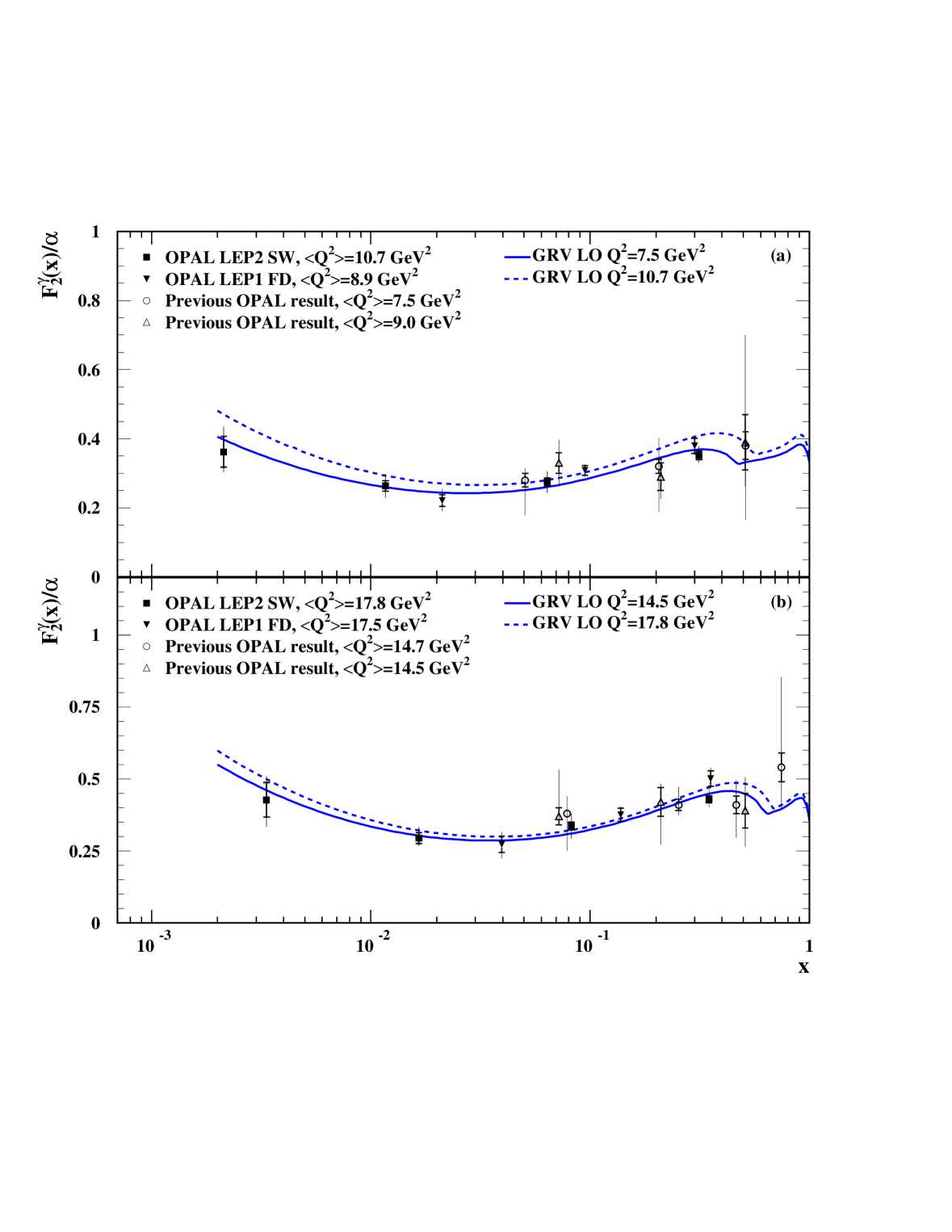
Figure 19: The measurement of $F_{2}^{\gamma}/\mbox{$\alpha$ }$ using the LEP1 FD and LEP2 SW samples for $\langle\mbox{$Q^{2}$}\rangle$ values of (a) 8.9 (10.7) and (b) 17.5 (17.8) $\rm GeV^{2}$ for LEP1 (LEP2). Also shown are the previous OPAL results in these $Q^{2}$ ranges, which were unfolded with HERWIG 5.8d ($\langle\mbox{$Q^{2}$}\rangle$=7.5 $\rm GeV^{2}$ and $\langle\mbox{$Q^{2}$}\rangle$=14.7 $\rm GeV^{2}$) and HERWIG 5.9 ($\langle\mbox{$Q^{2}$}\rangle$=9.0 $\rm GeV^{2}$ and $\langle\mbox{$Q^{2}$}\rangle$=14.5 $\rm GeV^{2}$) using a linear $x$ scale. For each point, the inner error bars show the statistical error and the full error bars show the total error. The positions of the new OPAL points are as given in Table 6. The other points with closed symbols are shown at the centre of the $\log(x)$ bin, and those with open symbols are shown at the average $x$ value of the bin. The curves show the GRV LO structure function.

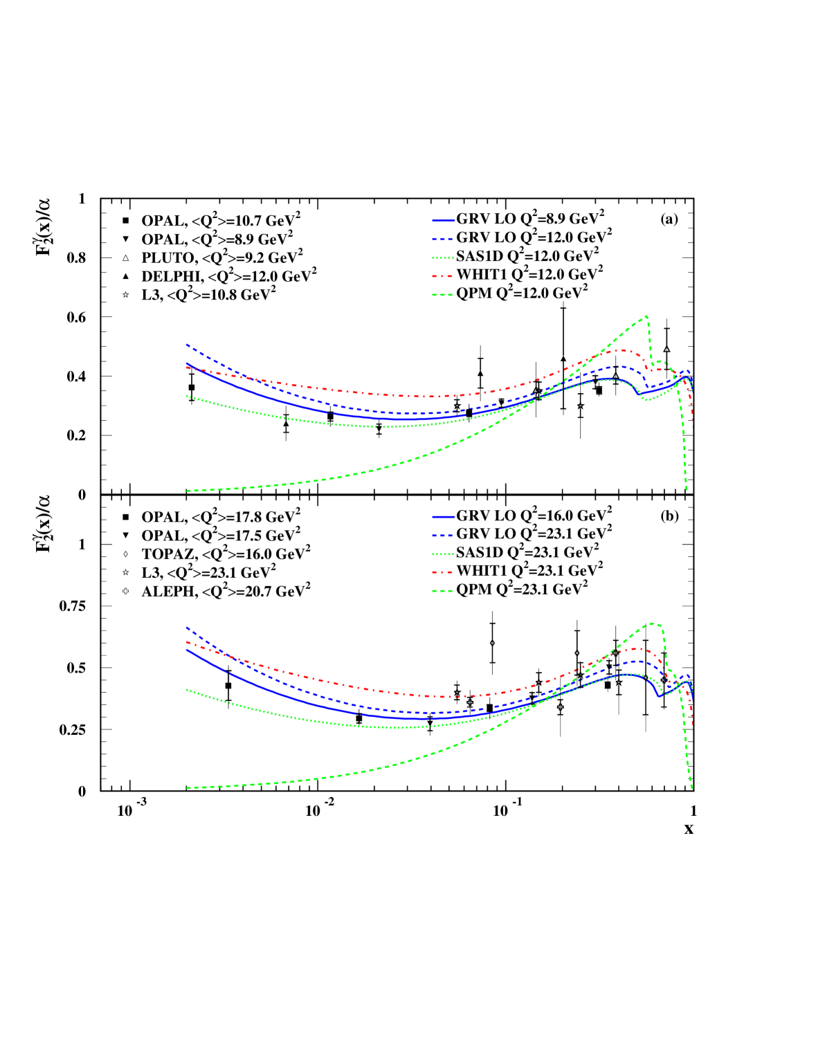
Figure 21: The measurement of $F_{2}^{\gamma}/\mbox{$\alpha$ }$ using the LEP1 FD and LEP2 SW samples for $\langle\mbox{$Q^{2}$}\rangle$ values of (a) 8.9 (10.7) and (b) 17.5 (17.8) $\rm GeV^{2}$ for LEP1 (LEP2). Also shown is a selection of results from other experiments: ALEPH [19], DELPHI [17], L3 [18], PLUTO [10], and TOPAZ [15]. For each point, the inner error bars show the statistical error and the full error bars show the total error. The positions of the new OPAL points are as given in Table 6. The other points with closed symbols are shown at the centre of the $\log(x)$ bin, and those with open symbols are shown at the average $x$ value of the bin. The curves show the GRV LO, SaS1D, WHIT1 and QPM structure functions.

References

- [1] V. M. Budnev et al., Phys. Rep. 15 (1975) 181.
-
[2]
E. Witten, Nucl. Phys. B120 (1977) 189;
A. Cordier and P. M. Zerwas, in ECFA Workshop on LEP200, Vol. 1, CERN 87-08, ECFA 87/108, eds A. Böhm and W. Hoogland (1987) 242;
R. Nisius, The Photon Structure from Deep Inelastic Electron Photon Scattering, hep-ex/9912049 (1999), to be published in Phys. Rep. - [3] C. Berger and W. Wagner, Phys. Rep. 146 (1987) 1.
-
[4]
H1 Collaboration, S. Aid et al., Nucl. Phys. B470 (1996) 3;
H1 Collaboration, C. Adloff et al., Nucl. Phys. B497 (1997) 3. -
[5]
ZEUS Collaboration,
M. Derrick et al., Z. Phys. C72 (1996) 399;
ZEUS Collaboration, J. Breitweg et al., Eur. Phys. J. C7 (1999) 609. -
[6]
M. Glück, E. Reya and A. Vogt, Phys. Rev. D45 (1992) 3986;
M. Glück, E. Reya and A. Vogt, Phys. Rev. D46 (1992) 1973. - [7] G. A. Schuler and T. Sjöstrand, Z. Phys. C68 (1995) 607.
- [8] K. Hagiwara et al., Phys. Rev. D51 (1995) 3197.
-
[9]
J. H. Field, F. Kapusta, L. Poggioli, Phys. Lett. B181 (1986) 362;
J. H. Field, F. Kapusta, L. Poggioli, Z. Phys. C36 (1987) 121;
F. Kapusta, Z. Phys. C42 (1989) 225. -
[10]
PLUTO Collaboration, C. Berger et al., Phys. Lett.
B107 (1981) 168;
PLUTO Collaboration, C. Berger et al., Phys. Lett. B142 (1984) 111;
PLUTO Collaboration, C. Berger et al., Nucl. Phys. B281 (1987) 365. -
[11]
JADE Collaboration, W. Bartel et al., Phys. Lett B121 (1983) 203;
JADE Collaboration, W. Bartel et al., Z. Phys. C24 (1984) 231. - [12] TASSO Collaboration, M. Althoff et al., Z. Phys. C31 (1986) 527.
-
[13]
TPC/2 Collaboration,
H. Aihara et al., Z. Phys. C34 (1987) 1;
TPC/2 Collaboration, H. Aihara et al., Phys. Rev. Lett. 58 (1987) 97. -
[14]
AMY Collaboration, T. Sasaki et al., Phys. Lett. B252 (1990) 491;
AMY Collaboration, S. K. Sahu et al., Phys. Lett. B346 (1995) 208;
AMY Collaboration, T. Kojima et al., Phys. Lett. B400 (1997) 395. - [15] TOPAZ Collaboration, K. Muramatsu et al., Phys. Lett. B332 (1994) 477.
-
[16]
OPAL Collaboration, R. Akers et al., Z. Phys. C61 (1994) 199;
OPAL Collaboration, K. Ackerstaff et al., Z. Phys C74 (1997) 33;
OPAL Collaboration, K. Ackerstaff et al., Phys. Lett. B411 (1997) 387;
OPAL Collaboration, K. Ackerstaff et al., Phys. Lett. B412 (1997) 225. - [17] DELPHI Collaboration, P. Abreu et al., Z. Phys. C69 (1996) 223.
-
[18]
L3 Collaboration, M. Acciarri et al., Phys. Lett. B436 (1998) 403;
L3 Collaboration, M. Acciarri et al., Phys. Lett. B447 (1999) 147. - [19] ALEPH Collaboration, D. Barate et al., Phys. Lett. B458 (1999) 152.
- [20] OPAL Collaboration, G. Abbiendi et al., Inclusive Production of D∗± Mesons in Photon-Photon Collisions at and GeV and a First Measurement of , CERN-EP/99-157 (1999), Accepted by Eur. Phys. J. C.
-
[21]
OPAL Collaboration, K. Ahmet et al., Nucl. Instr. and Meth. A305 (1991) 275;
P. P. Allport et al., Nucl. Instr. and Meth. A324 (1993) 34;
P. P. Allport et al., Nucl. Instr. and Meth. A346 (1994) 476;
B. E. Anderson et al., IEEE Transactions on Nuclear Science 41 (1994) 845. - [22] OPAL Collaboration, G. Alexander et al., Phys. Lett. B377 (1996) 181.
- [23] J. Allison et al., Nucl. Instr. and Meth. A317 (1992) 47.
- [24] G. Marchesini et al., Comp. Phys. Comm 67 (1992) 465.
-
[25]
J. A. Lauber, L. Lönnblad and M. H. Seymour,
Proceedings of Photon ’97,
10–15 May 1997, eds A. Buijs, F.C. Erné, World Scientific (1997) 52;
S. Cartwright, M.H. Seymour et al., J. Phys. G24 (1998) 457;
A. Finch, Proceedings of Photon ’99, 23–27 May 1999, ed S. Söldner Rembold, Nucl. Phys. B (Proc. Suppl.), Vol 82 (2000), 156. -
[26]
R. Engel, Z. Phys. C66 (1995) 203;
R. Engel, J. Ranft and S. Roesler, Phys. Rev. D52 (1995) 1459;
R. Engel and J. Ranft, Phys. Rev. D54 (1996) 4244. - [27] A. Buijs et al., Comp. Phys. Comm. 79 (1994) 523.
- [28] ZEUS Collaboration, M. Derrick et al., Phys. Lett. B354 (1995) 163.
-
[29]
H. Plothow-Besch, PDFLIB, User’s Manual, CERN Program Library entry W5051;
H. Plothow-Besch, Comp. Phys. Comm. 75 (1993) 396. -
[30]
J. A. M. Vermaseren, Nucl. Phys. B229 (1983) 347;
R. Bhattacharya, G. Grammer Jr. and J. Smith, Phys. Rev. D15 (1977) 3267;
J. Smith, J.A.M. Vermaseren and G. Grammer Jr., Phys. Rev. D15 (1977) 3280;
J. A. M. Vermaseren, J. Smith and G. Grammer Jr., Phys. Rev. D19 (1979) 137. -
[31]
T. Sjöstrand, Comp. Phys. Comm. 39 (1986) 347;
T. Sjöstrand and M. Bengtsson, Comp. Phys. Comm. 43 (1987) 367;
T. Sjöstrand, Comp. Phys. Comm. 82 (1994) 74. - [32] S. Jadach, B. F. L. Ward and Z. Wa̧s, Comp. Phys. Comm. 79 (1994) 503.
- [33] J. Hilgart, R. Kleiss and F. Le Diberder, Comp. Phys. Comm. 75 (1993) 191.
-
[34]
T. Sjöstrand, Comp. Phys. Comm. 82 (1994) 74;
T. Sjöstrand, PYTHIA 5.7 and JETSET 7.4: Physics and Manual, CERN-TH/93-7112. -
[35]
M. Landrø, K.J. Mork, and H.A. Olsen, Phys. Rev. D36 (1987) 44;
F.A. Berends, P.H. Daverveldt, and R. Kleiss, Nucl. Phys. B253 (1985) 441;
F.A. Berends, P.H. Daverveldt, and R. Kleiss, Comp. Phys. Comm. 40 (1986) 285. -
[36]
E. Laenen and G.A. Schuler, Phys. Lett. B374 (1996) 217;
E. Laenen and G.A. Schuler, Model-independent QED corrections to photon structure-function measurements, in Photon ’97, Incorporating the XIth International Workshop on GammaGamma Collisions, Egmond aan Zee, 10-15 May, 1997, edited by A. Buijs and F.C. Erné, pages 57–62, World Scientific, 1998. -
[37]
M. Glück, E. Reya and M. Stratmann, Phys. Rev. D51 (1995) 3220;
M. Glück, E. Reya and M. Stratmann, Phys. Rev. D54 (1996) 5515. - [38] G. A. Schuler and T. Sjöstrand, Phys. Lett. B376 (1996) 193.
- [39] M. Drees and R. M. Godbole, Phys. Rev. D50 (1994) 3124.
- [40] A. Höcker, V. Kartvelishvili, Nucl. Instr. and Meth. A372 (1996) 469.
-
[41]
V. Blobel,
Unfolding Methods in High-Energy Physics Experiments,
DESY-84-118 (1984);
V. Blobel, Proceedings of the 1984 CERN School of Computing, Aiguablava, Spain, 9–22 September 1984, CERN 85-09 (1985). - [42] G. D’Agostini, Nucl. Instr. and Meth. A362 (1996) 489.
- [43] L. Lönnblad et al., CERN 96-01, Physics at LEP2, eds G. Altarelli, T. Sjöstrand and F. Zwirner (1996) Vol. 2, p. 201.
- [44] OPAL Collaboration, K. Ackerstaff et al., Eur. Phys. J. C5 (1998) 411.