Study of exclusive two-body $B^{0}$ meson decays to charmonium

Abstract

We present a study of three $B^{0}$ decay modes useful for time-dependent $CP$ asymmetry measurements. From a sample of $9.7\times 10^{6}$ $B\overline{B}$ meson pairs collected with the CLEO detector, we have reconstructed $B^{0}\to J/\psi\,K^{0}_{S}$, $B^{0}\to\chi_{c1}\,K^{0}_{S}$, and $B^{0}\to J/\psi\,\pi^{0}$ decays. The latter two decay modes have been observed for the first time. We describe a $K^{0}_{S}\to\pi^{0}\pi^{0}$ detection technique and its application to the reconstruction of the decay $B^{0}\to J/\psi\,K^{0}_{S}$. Combining the results obtained using $K^{0}_{S}\to\pi^{+}\pi^{-}$ and $K^{0}_{S}\to\pi^{0}\pi^{0}$ decays, we determine ${\cal B}(B^{0}\to J/\psi\,K^{0})=(9.5\pm 0.8\pm 0.6)\times 10^{-4}$, where the first uncertainty is statistical and the second one is systematic. We also obtain ${\cal B}(B^{0}\to\chi_{c1}\,K^{0})=(3.9^{+1.9}_{-1.3}\pm 0.4)\times 10^{-4}$ and ${\cal B}(B^{0}\to J/\psi\,\pi^{0})=(2.5^{+1.1}_{-0.9}\pm 0.2)\times 10^{-5}$.

$CP$ violation arises naturally in the Standard Model with three quark generations [1]; however, it still remains one of the least experimentally constrained sectors of the Standard Model. Measurements of time-dependent rate asymmetries in the decays of neutral $B$ mesons will provide an important test of the Standard Model mechanism for $CP$ violation [2].

In this Article, we present a study of $B^{0}\to J/\psi\,K^{0}_{S}$, $B^{0}\to\chi_{c1}\,K^{0}_{S}$, and $B^{0}\to J/\psi\,\pi^{0}$ decays. The latter two decay modes have been observed for the first time. We describe a $K^{0}_{S}\to\pi^{0}\pi^{0}$ detection technique and its application to the reconstruction of the decay $B^{0}\to J/\psi\,K^{0}_{S}$.

The measurement of the $CP$ asymmetry in $B^{0}(\overline{B}^{0})\to J/\psi\,K^{0}_{S}$ decays probes the relative weak phase between the $B^{0}-\overline{B}^{0}$ mixing amplitude and the $b\to c\bar{c}s$ decay amplitude [3]. In the Standard Model this measurement determines $\sin 2\beta$, where $\beta\equiv{\rm Arg}\left(-V_{cd}V^{*}_{cb}/V_{td}V^{*}_{tb}\right)$. A measurement of $\sin 2\beta$ with $B^{0}(\overline{B}^{0})\to\chi_{c1}\,K^{0}_{S}$ decays is as theoretically clean as one with $B^{0}(\overline{B}^{0})\to J/\psi\,K^{0}_{S}$.

For the purposes of $CP$ violation measurements, the $B^{0}\to J/\psi\,\pi^{0}$ decay is similar to $B^{0}\to D^{+}\,D^{-}$: both decays are governed by the $b\to c\bar{c}d$ quark transition, and both final states are $CP$ eigenstates of the same $CP$ sign. A recent search for the $B^{0}\to D^{+}\,D^{-}$ decay at CLEO established an upper limit on ${\cal B}(B^{0}\to D^{+}\,D^{-})$ [4]. If the penguin ($b\to dc\bar{c}$) amplitude is negligible compared to the tree ($b\to c\bar{c}d$) amplitude, then the measurement the $CP$ asymmetry in $B^{0}(\overline{B}^{0})\to J/\psi\,\pi^{0}$ decays allows a theoretically clean extraction of $\sin 2\beta$. The asymmetries measured with $J/\psi\,K^{0}_{S}$ and $J/\psi\,\pi^{0}$ final states should have exactly the same absolute values but opposite signs, thus providing a useful check for charge-correlated systematic bias in $B$-flavor tagging. If the ratio of penguin to tree amplitudes is not too small [5], then comparison of the measured asymmetries in $J/\psi\,K^{0}_{S}$ and $J/\psi\,\pi^{0}$ modes may allow a resolution of one of the two discrete ambiguities ($\beta\to\beta+\pi$) remaining after a $\sin 2\beta$ measurement [6].

The data were collected at the Cornell Electron Storage Ring (CESR) with two configurations of the CLEO detector called CLEO II [7] and CLEO II.V [8]. The components of the CLEO detector most relevant to this analysis are the charged particle tracking system, the CsI electromagnetic calorimeter, and the muon chambers. In CLEO II the momenta of charged particles are measured in a tracking system consisting of a 6-layer straw tube chamber, a 10-layer precision drift chamber, and a 51-layer main drift chamber, all operating inside a 1.5 T solenoidal magnet. The main drift chamber also provides a measurement of the specific ionization, $dE/dx$, used for particle identification. For CLEO II.V, the straw tube chamber was replaced with a 3-layer silicon vertex detector, and the gas in the main drift chamber was changed from an argon-ethane to a helium-propane mixture. The muon chambers consist of proportional counters placed at increasing depth in the steel absorber. We use 9.2 $\rm fb^{-1}$ of $e^{+}e^{-}$ data taken at the $\Upsilon(4S)$ resonance and 4.6 $\rm fb^{-1}$ taken 60 MeV below the $\Upsilon(4S)$ resonance. Two thirds of the data were collected with the CLEO II.V detector. The simulated event samples used in this analysis were generated with a GEANT-based [9] simulation of the CLEO detector response and were processed in a similar manner as the data.

We reconstruct both $J/\psi\to e^{+}e^{-}$ and $J/\psi\to\mu^{+}\mu^{-}$ decays and use identical $J/\psi$ selection criteria for all measurements described in this Article. Electron candidates are identified based on the ratio of the track momentum to the associated shower energy in the CsI calorimeter and on the $dE/dx$ measurement. The internal bremsstrahlung in the $J/\psi\to e^{+}e^{-}$ decay as well as the bremsstrahlung in the detector material produces a long radiative tail in the $e^{+}e^{-}$ invariant mass distribution and impedes efficient $J/\psi\to e^{+}e^{-}$ detection. We recover some of the bremsstrahlung photons by selecting the photon shower with the smallest opening angle with respect to the direction of the $e^{\pm}$ track evaluated at the interaction point, and then requiring this opening angle to be smaller than $5^{\circ}$. We therefore refer to the $e^{+}(\gamma)e^{-}(\gamma)$ invariant mass when we describe the $J/\psi\to e^{+}e^{-}$ reconstruction. For the $J/\psi\to\mu^{+}\mu^{-}$ reconstruction, one of the muon candidates is required to penetrate the steel absorber to a depth greater than 3 nuclear interaction lengths. We relax the absorber penetration requirement for the second muon candidate if it is not expected to reach a muon chamber either because its energy is too low or because it does not point to a region of the detector covered by the muon chambers. For these muon candidates we require the ionization signature in the CsI calorimeter to be consistent with that of a muon.

We extensively use normalized variables, taking advantage of well-understood track and photon-shower four-momentum covariance matrices to calculate the expected resolution for each combination. The use of normalized variables allows uniform candidate selection criteria to be applied to the data collected with the CLEO II and CLEO II.V detector configurations. For example, the normalized $J/\psi\to\mu^{+}\mu^{-}$ mass is defined as $[M(\mu^{+}\mu^{-})-M_{J/\psi}]/\sigma(M)$, where $M_{J/\psi}$ is the world average value of the $J/\psi$ mass [10] and $\sigma(M)$ is the calculated mass resolution for that particular $\mu^{+}\mu^{-}$ combination. The average $\ell^{+}\ell^{-}$ invariant mass resolution is 12 MeV$/c^{2}$. The normalized mass distributions for the $J/\psi\to\ell^{+}\ell^{-}$ candidates are shown in Fig. 1. We require the normalized mass to be from $-10$ to $+3$ for the $J/\psi\to e^{+}e^{-}$ and from $-4$ to $+3$ for the $J/\psi\to\mu^{+}\mu^{-}$ candidates.

Photon candidates for $\chi_{c1}\to J/\psi\,\gamma$ and $\pi^{0}\to\gamma\gamma$ decays are required to have an energy of at least 30 MeV in the barrel region ($|\cos\theta_{\gamma}|<0.71$) and at least 50 MeV in the endcap region ($0.71<|\cos\theta_{\gamma}|<0.95$), where $\theta_{\gamma}$ is the angle between the beam axis and the candidate photon. To select the $\pi^{0}$ candidates for $B^{0}\to J/\psi\,\pi^{0}$ reconstruction, we require the normalized $\pi^{0}\to\gamma\gamma$ mass to be between $-5$ and $+4$. The average $\gamma\gamma$ invariant mass resolution for these $\pi^{0}$ candidates is 7 MeV$/c^{2}$. We perform a fit constraining the mass of each $\pi^{0}$ candidate to the world average value [10].

We reconstruct $\chi_{c1}$ in the $\chi_{c1}\to J/\psi\,\gamma$ decay mode. Most of the photons in $\Upsilon(4S)\to B\overline{B}$ events come from $\pi^{0}$ decays. We therefore do not use a photon if it can be paired with another photon to produce a $\pi^{0}$ candidate with the normalized $\pi^{0}\to\gamma\gamma$ mass between $-4$ and $+3$. The resolution in the $J/\psi\,\gamma$ invariant mass is 8 MeV$/c^{2}$. We select the $\chi_{c1}$ candidates with the normalized $\chi_{c1}\to J/\psi\,\gamma$ mass between $-4$ and $+3$ and perform a fit constraining the mass of each $\chi_{c1}$ candidate to the world average value [10].

The $K^{0}_{S}\to\pi^{+}\pi^{-}$ candidates are selected from pairs of tracks forming well-measured displaced vertices. We refit the daughter pion tracks taking into account the position of the displaced vertex and constrain them to originate from the measured vertex. The resolution in the $\pi^{+}\pi^{-}$ invariant mass is 4 MeV$/c^{2}$. We select the $K^{0}_{S}\to\pi^{+}\pi^{-}$ candidates with the normalized $K^{0}_{S}\to\pi^{+}\pi^{-}$ mass between $-4$ and $+4$ and perform a fit constraining the mass of each $K^{0}_{S}$ candidate to the world average value [10].

In order to increase our $B^{0}\to J/\psi\,K^{0}_{S}$ sample, we also reconstruct $K^{0}_{S}\to\pi^{0}\pi^{0}$ decays. The average flight distance for the $K^{0}_{S}$ from $B^{0}\to J/\psi\,K^{0}_{S}$ decay is 9 cm. We find the $K^{0}_{S}$ decay vertex using only the calorimeter information and the known position of the $e^{+}e^{-}$ interaction point. The $K^{0}_{S}$ flight direction is calculated as the line passing through the $e^{+}e^{-}$ interaction point and the center of energy of the four photon showers in the calorimeter. The $K^{0}_{S}$ decay vertex is defined as the point along the $K^{0}_{S}$ flight direction for which the product $f[M(\gamma_{1}\gamma_{2})]\times f[M(\gamma_{3}\gamma_{4})]$ is maximal. In the above expression, $M(\gamma_{1}\gamma_{2})$ and $M(\gamma_{3}\gamma_{4})$ are the diphoton invariant masses recalculated assuming a particular $K^{0}_{S}$ decay point and $f(M)$ is the $\pi^{0}$ mass lineshape obtained from the simulation where we use the known $K^{0}_{S}$ decay vertex. For simulated events, the $K^{0}_{S}$ flight distance is found without bias with a resolution of 5 cm. The uncertainty in the $K^{0}_{S}$ decay vertex position arising from the $K^{0}_{S}$ direction approximation is much smaller than the resolution of the flight distance. We select the $K^{0}_{S}$ candidates by requiring the reconstructed $K^{0}_{S}$ decay length to be in the range from $-10$ to $+60$ cm. After the $K^{0}_{S}$ decay vertex is found, we select the $K^{0}_{S}\to\pi^{0}\pi^{0}$ candidates by requiring $-15<M(\gamma\gamma)-M_{\pi^{0}}<10$ MeV/$c^{2}$ for both photon pairs. Then we perform a kinematic fit simultaneously constraining $M(\gamma_{1}\gamma_{2})$ and $M(\gamma_{3}\gamma_{4})$ to the world average value of the $\pi^{0}$ mass [10]. The resulting $K^{0}_{S}$ mass resolution is 12 MeV/$c^{2}$. We select the $K^{0}_{S}\to\pi^{0}\pi^{0}$ candidates with the normalized $K^{0}_{S}\to\pi^{0}\pi^{0}$ mass between $-3$ and $+3$ and perform a fit constraining the mass of each $K^{0}_{S}$ candidate to the world average value [10]. The $K^{0}_{S}\to\pi^{0}\pi^{0}$ detection efficiency is determined from simulation. The systematic uncertainty associated with this determination can be reliably estimated by comparing the $K^{0}_{S}\to\pi^{0}\pi^{0}$ and $K^{0}_{S}\to\pi^{+}\pi^{-}$ yields for inclusive $K^{0}_{S}$ candidates in data and in simulated events.

The $B^{0}$ candidates are selected by means of two observables. The first observable is the difference between the energy of the $B^{0}$ candidate and the beam energy, $\Delta E\equiv E(B^{0})-E_{\rm beam}$. The average $\Delta E$ resolution for each decay mode is listed in Table I. We use the normalized $\Delta E$ for candidate selection and require $|\Delta E|/\sigma(\Delta E)<3$ for $B^{0}\to J/\psi\,K^{0}_{S}$ and $B^{0}\to\chi_{c1}\,K^{0}_{S}$ candidates with $K^{0}_{S}\to\pi^{+}\pi^{-}$. To account for a low-side $\Delta E$ tail arising from the energy leakage in the calorimeter, we require $-5<\Delta E/\sigma(\Delta E)<3$ for $B^{0}\to J/\psi\,K^{0}_{S}$ with $K^{0}_{S}\to\pi^{0}\pi^{0}$ and $-4<\Delta E/\sigma(\Delta E)<3$ for $B^{0}\to J/\psi\,\pi^{0}$ candidates. The second observable is the beam-constrained $B$ mass, $M(B)\equiv\sqrt{E^{2}_{\rm beam}-p^{2}(B)}$, where $p(B)$ is the magnitude of the $B^{0}$ candidate momentum. The resolution in $M(B)$ is dominated by the beam energy spread for all the decay modes under study and varies from 2.7 to 3.0 MeV/$c^{2}$ depending on the mode. We use the normalized $M(B)$ for candidate selection and require $|M(B)-M_{B}|/\sigma(M)<3$, where $M_{B}$ is the nominal $B^{0}$ meson mass. The $\Delta E$ vs. $M(B)$ distributions together with the projections on the $M(B)$ axis are shown in Fig. 2. The number of $B^{0}$ candidates selected in each decay mode is listed in Table I.

Backgrounds can be divided into two categories. The first category is the background from those exclusive $B$ decays that tend to produce a peak in the signal region of the $M(B)$ distribution. We identify these exclusive $B$ decays and estimate their contributions to background using simulated events with the normalizations determined from the known branching fractions or from our data. The second category is the combinatorial background from $B\overline{B}$ and continuum non-$B\overline{B}$ events. To estimate the combinatorial background, we fit the $M(B)$ distribution in the region from 5.1 to 5.3 GeV/$c^{2}$. As a consistency check, we also estimate the combinatorial background using high-statistics samples of simulated $\Upsilon(4S)\to B\overline{B}$ and non-$B\overline{B}$ continuum events together with the data collected below the $B\overline{B}$ production threshold. The total estimated backgrounds are listed in Table I. Below we describe the background estimation for each decay channel under study.

Background for $B^{0}\to J/\psi\,K^{0}_{S}$ with $K^{0}_{S}\to\pi^{+}\pi^{-}$. Only combinatorial background contributes, with the total background estimated to be $0.3\pm 0.2$ events.

Background for $B^{0}\to J/\psi\,K^{0}_{S}$ with $K^{0}_{S}\to\pi^{0}\pi^{0}$. The combinatorial background is estimated to be $0.5\pm 0.2$ events. The other background source is $B\to J/\psi\,K^{*}$ [11], with $K^{*}\to K\pi^{0}$ or $K^{*}\to K^{0}_{S}\pi$ with $K^{0}_{S}\to\pi^{0}\pi^{0}$. The background from these decays is estimated to be $0.6\pm 0.2$ events.

Background for $B^{0}\to\chi_{c1}\,K^{0}_{S}$. The combinatorial background is estimated to be $0.5\pm 0.3$ events. We estimate the background from $B$ decays to the $J/\psi\,K^{0}_{S}\pi$ final state from the samples of simulated events, with the normalizations obtained from the fits to the $M(K\pi)$ distributions for $B^{+}\to J/\psi\,K^{0}_{S}\pi^{+}$ and $B^{0}\to J/\psi\,K^{-}\pi^{+}$ candidates in data. The background from $B\to J/\psi\,K^{0}_{S}\pi$ is estimated to be $0.41\pm 0.07$ events, and is dominated by $B\to J/\psi\,K^{*}$ decays with $K^{*}\to K^{0}_{S}\pi$. We find no evidence for $B\to\chi_{c2}\,K$ production and estimate the background from $B^{0}\to\chi_{c2}\,K^{0}_{S}$ to be $0.01\pm 0.01$ events.

Background for $B^{0}\to J/\psi\,\pi^{0}$. The combinatorial background is estimated to be $0.4^{+0.5}_{-0.3}$ events. The $\Delta E$ resolution is good enough to render negligible the background from any of the Cabibbo-allowed $B\to J/\psi K\pi^{0}(X)$ decays, where at least a kaon mass is missing from the energy sum. The background from $B^{0}\to J/\psi\,K^{0}_{S}$ decays with $K^{0}_{S}\to\pi^{0}\pi^{0}$ is estimated to be $0.38\pm 0.05$ events. We estimate the background from $B$ decays to the $J/\psi\,\pi\pi^{0}$ final state from the samples of simulated events, with the normalizations obtained from the fits to the $M(\pi\pi)$ distributions for $B^{+}\to J/\psi\,\pi^{+}\pi^{0}$ and $B^{0}\to J/\psi\,\pi^{0}\pi^{0}$ candidates in data. The background from $B\to J/\psi\,\pi^{0}\pi$ is estimated to be $0.2\pm 0.2$ events, and is dominated by $B^{+}\to J/\psi\,\rho^{+}$ decays.

We use the Feldman-Cousins approach  [12] to assign the 68% C.L. intervals for the signal mean for the three low-statistics decay modes ($B^{0}\to\chi_{c1}\,K^{0}_{S}$, $B^{0}\to J/\psi\,\pi^{0}$, and $B^{0}\to J/\psi\,K^{0}_{S}$ with $K^{0}_{S}\to\pi^{0}\pi^{0}$). We assume ${\cal B}(\Upsilon(4S)\to B^{0}{\overline{B}^{0}})={\cal B}(\Upsilon(4S)\to B^{+}B^{-})$ for all branching fractions in this Article. We use the following branching fractions for the secondary decays: ${\cal B}(J/\psi\to\ell^{+}\ell^{-})=(5.894\pm 0.086)\%$ [13], ${\cal B}(\chi_{c1}\to J/\psi\gamma)=(27.3\pm 1.6)\%$ [10], ${\cal B}(K^{0}_{S}\to\pi^{+}\pi^{-})=(68.61\pm 0.28)\%$ [10], and ${\cal B}(K^{0}_{S}\to\pi^{0}\pi^{0})=(31.39\pm 0.28)\%$ [10]. The reconstruction efficiencies are determined from simulation. The resulting branching fractions are listed in Table I. Combining the results for the two $K^{0}_{S}$ modes used in $B^{0}\to J/\psi\,K^{0}_{S}$ reconstruction and taking into account correlated systematic uncertainties, we obtain ${\cal B}(B^{0}\to J/\psi\,K^{0})=(9.5\pm 0.8\pm 0.6)\times 10^{-4}$. The measurements of ${\cal B}(B^{0}\to J/\psi\,K^{0})$, ${\cal B}(B^{0}\to\chi_{c1}\,K^{0})$, and ${\cal B}(B^{0}\to J/\psi\,\pi^{0})$ reported in this Article supersede the previous CLEO results [14].

The systematic uncertainties in the branching fraction measurements include contributions from the uncertainty in the number of $B\overline{B}$ pairs (2%), tracking efficiencies (1% per charged track), photon detection efficiency (2.5%), lepton detection efficiency (3% per lepton), $K^{0}_{S}\to\pi^{+}\pi^{-}$ finding efficiency (2%), $K^{0}_{S}\to\pi^{0}\pi^{0}$ finding efficiency (5%), background subtraction ($0.01-5.5\%$, see Table I), statistics of the simulated event samples ($0.6-1.0\%$), and the uncertainties on the branching fractions of secondary decays (see Table I).

In summary, we have studied three $B^{0}$ decay modes useful for the measurement of $\sin 2\beta$. We report the first observation and measure branching fractions of the $B^{0}\to\chi_{c1}\,K^{0}$ and $B^{0}\to J/\psi\,\pi^{0}$ decays. We describe a $K^{0}_{S}\to\pi^{0}\pi^{0}$ detection technique and its application to the reconstruction of the decay $B^{0}\to J/\psi\,K^{0}_{S}$. We measure the branching fraction for $B^{0}\to J/\psi\,K^{0}$ decays with $K^{0}_{S}$ mesons reconstructed in both $\pi^{+}\pi^{-}$ and $\pi^{0}\pi^{0}$ decay modes.

We gratefully acknowledge the effort of the CESR staff in providing us with excellent luminosity and running conditions. This work was supported by the National Science Foundation, the U.S. Department of Energy, the Research Corporation, the Natural Sciences and Engineering Research Council of Canada, the A.P. Sloan Foundation, the Swiss National Science Foundation, the Texas Advanced Research Program, and the Alexander von Humboldt Stiftung.

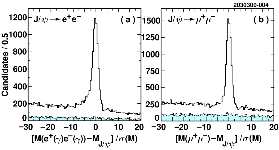
FIG. 1.: Normalized invariant mass of the (a) $J/\psi\to e^{+}e^{-}$ and (b) $J/\psi\to\mu^{+}\mu^{-}$ candidates in data. The momentum of the $J/\psi$ candidates is required to be less than 2 GeV/$c$, which is slightly above the maximal $J/\psi$ momentum in $B\to J/\psi\,\pi$ decays. The shaded histogram represents the luminosity-scaled data taken 60 MeV below the $\Upsilon(4S)$ showing the level of background from non-$B\overline{B}$ events.

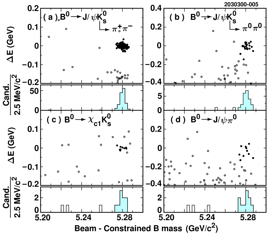
FIG. 2.: The $\Delta E$ vs. $M(B)$ distribution for (a) $B^{0}\to J/\psi\,K^{0}_{S}$ with $K^{0}_{S}\to\pi^{+}\pi^{-}$, (b) $B^{0}\to J/\psi\,K^{0}_{S}$ with $K^{0}_{S}\to\pi^{0}\pi^{0}$, (c) $B^{0}\to\chi_{c1}\,K^{0}_{S}$, and (d) $B^{0}\to J/\psi\,\pi^{0}$ candidates. The signal candidates, selected using normalized $\Delta E$ and $M(B)$ variables, are shown by filled circles. Below each $\Delta E$ vs. $M(B)$ plot, we show the projection on the $M(B)$ axis with the $\Delta E$ requirement applied. The shaded parts of the histograms represent the candidates that pass the $|M(B)-M_{B}|/\sigma(M)<3$ requirement.

TABLE I.: Number of signal candidates, estimated background, average $\Delta E$ resolution, product of secondary branching fractions (${\cal B}_{s}$), detection efficiency, and measured branching fraction. Row 1 contains the combined value of ${\cal B}(B^{0}\to J/\psi\,K^{0})$, rows 2 and 3 contain the individual results for the two $K^{0}_{S}$ decay modes.

Decay	Signal	Total	$\sigma(\Delta E)$	${\cal B}_{s}$	Efficiency	Branching
mode	candidates	background	(MeV)	$(\%)$	$(\%)$	fraction $(\times 10^{-4})$
$B^{0}\to J/\psi\,K^{0}$						$9.5\pm 0.8\pm 0.6$
$K^{0}_{S}\to\pi^{+}\pi^{-}$	142	$0.3\pm 0.2$	11	$4.04\pm 0.06$	$37.0\pm 2.3$	$9.8\pm 0.8\pm 0.7$
$K^{0}_{S}\to\pi^{0}\pi^{0}$	22	$1.1\pm 0.3$	25a	$1.85\pm 0.03$	$13.9\pm 1.1$b	$8.4^{+2.1}_{-1.9}\pm 0.7$
$B^{0}\to\chi_{c1}\,K^{0}$	9	$0.9\pm 0.3$	10	$1.10\pm 0.07$	$19.2\pm 1.3$	$3.9^{+1.9}_{-1.3}\pm 0.4$
$B^{0}\to J/\psi\,\pi^{0}$	10	$1.0\pm 0.5$	28a	$11.8\pm 0.2$	$31.4\pm 2.2$b	$0.25^{+0.11}_{-0.09}\pm 0.02$

REFERENCES

- [1] N. Cabibbo, Phys. Rev. Lett. 10, 531 (1963); M. Kobayashi and T. Maskawa, Prog. Theor. Phys. 49, 652 (1973).
- [2] For a recent review see Y. Nir, lectures given at 27th SLAC Summer Institute on Particle Physics (SSI 99), Stanford, California, Report No. IASSNS-HEP-99-104, hep-ph/9911321.
- [3] OPAL Collaboration, K. Ackerstaff et al., Eur. Phys. J. C 5, 379 (1998); CDF Collaboration, T. Affolder et al., Phys. Rev. D 61, 072005 (2000); ALEPH Collaboration, R. Barate et al., contribution to the 3rd Int. Conf. on Physics and violation in Taipei, Taiwan, Report No. ALEPH 99-099, CONF-99-054 (1999).
- [4] CLEO Collaboration, E. Lipeles et al., Report No. CLNS 00/1663 (to be published in Phys. Rev. D).
- [5] M. Ciuchini et al., Phys. Rev. Lett. 79, 978 (1997).
- [6] Y. Grossman and H. R. Quinn, Phys. Rev. D 56, 7259 (1997).
- [7] CLEO Collaboration, Y. Kubota et al., Nucl. Instrum. Meth. Phys. Res. A 320, 66 (1992).
- [8] T.S. Hill, Nucl. Instrum. Meth. Phys. Res. A 418, 32 (1998).
- [9] CERN Program Library Long Writeup W5013 (1993).
- [10] Particle Data Group, C. Caso et al., Eur. Phys. J. C 3, 1 (1998).
- [11] We refer to as . Unless otherwise noted, is either or ; similarly is either or . Charge conjugation is implied.
- [12] G.J. Feldman and R.D. Cousins, Phys. Rev. D 57, 3873 (1998).
- [13] BES Collaboration, J. Z. Bai et al., Phys. Rev. D 58, 092006 (1998).
- [14] CLEO Collaboration, C. P. Jessop et al., Phys. Rev. Lett. 79, 4533 (1997); CLEO Collaboration, M. S. Alam et al., Phys. Rev. D 50, 43 (1994); CLEO Collaboration, M. Bishai et al., Phys. Lett. B 369, 186 (1996).