Measurements of Charm Fragmentation into $D_{s}^{*+}$ and $D_{s}^{+}$ in $e^{+}e^{-}$ Annihilations at $\sqrt{s}=10.5$ GeV

Abstract

A study of charm fragmentation into $D_{s}^{*+}$ and $D_{s}^{+}$ in $e^{+}e^{-}$ annihilations at $\sqrt{s}=10.5$ GeV is presented. This study using $4.72\pm 0.05$ fb^-1 of CLEO II data reports measurements of the cross-sections $\sigma(D_{s}^{*+})$ and $\sigma(D_{s}^{+})$ in momentum regions above $x=0.44$, where $x$ is the $D_{s}$ momentum divided by the maximum kinematically allowed $D_{s}$ momentum. The $D_{s}$ vector to vector plus pseudoscalar production ratio is measured to be $P_{V}(x(D_{s}^{+})>0.44)=0.44\pm 0.04$.

R. A. Briere,¹ B. H. Behrens,² W. T. Ford,² A. Gritsan,² H. Krieg,² J. Roy,² J. G. Smith,² J. P. Alexander,³ R. Baker,³ C. Bebek,³ B. E. Berger,³ K. Berkelman,³ F. Blanc,³ V. Boisvert,³ D. G. Cassel,³ M. Dickson,³ P. S. Drell,³ K. M. Ecklund,³ R. Ehrlich,³ A. D. Foland,³ P. Gaidarev,³ L. Gibbons,³ B. Gittelman,³ S. W. Gray,³ D. L. Hartill,³ B. K. Heltsley,³ P. I. Hopman,³ C. D. Jones,³ D. L. Kreinick,³ T. Lee,³ Y. Liu,³ T. O. Meyer,³ N. B. Mistry,³ C. R. Ng,³ E. Nordberg,³ J. R. Patterson,³ D. Peterson,³ D. Riley,³ J. G. Thayer,³ P. G. Thies,³ B. Valant-Spaight,³ A. Warburton,³ P. Avery,⁴ M. Lohner,⁴ C. Prescott,⁴ A. I. Rubiera,⁴ J. Yelton,⁴ J. Zheng,⁴ G. Brandenburg,⁵ A. Ershov,⁵ Y. S. Gao,⁵ D. Y.-J. Kim,⁵ R. Wilson,⁵ T. E. Browder,⁶ Y. Li,⁶ J. L. Rodriguez,⁶ H. Yamamoto,⁶ T. Bergfeld,⁷ B. I. Eisenstein,⁷ J. Ernst,⁷ G. E. Gladding,⁷ G. D. Gollin,⁷ R. M. Hans,⁷ E. Johnson,⁷ I. Karliner,⁷ M. A. Marsh,⁷ M. Palmer,⁷ C. Plager,⁷ C. Sedlack,⁷ M. Selen,⁷ J. J. Thaler,⁷ J. Williams,⁷ K. W. Edwards,⁸ R. Janicek,⁹ P. M. Patel,⁹ A. J. Sadoff,¹⁰ R. Ammar,¹¹ P. Baringer,¹¹ A. Bean,¹¹ D. Besson,¹¹ R. Davis,¹¹ S. Kotov,¹¹ I. Kravchenko,¹¹ N. Kwak,¹¹ X. Zhao,¹¹ S. Anderson,¹² V. V. Frolov,¹² Y. Kubota,¹² S. J. Lee,¹² R. Mahapatra,¹² J. J. O’Neill,¹² R. Poling,¹² T. Riehle,¹² A. Smith,¹² S. Ahmed,¹³ M. S. Alam,¹³ S. B. Athar,¹³ L. Jian,¹³ L. Ling,¹³ A. H. Mahmood,^13, M. Saleem,¹³ S. Timm,¹³ F. Wappler,¹³ A. Anastassov,¹⁴ J. E. Duboscq,¹⁴ K. K. Gan,¹⁴ C. Gwon,¹⁴ T. Hart,¹⁴ K. Honscheid,¹⁴ H. Kagan,¹⁴ R. Kass,¹⁴ J. Lorenc,¹⁴ H. Schwarthoff,¹⁴ E. von Toerne,¹⁴ M. M. Zoeller,¹⁴ S. J. Richichi,¹⁵ H. Severini,¹⁵ P. Skubic,¹⁵ A. Undrus,¹⁵ M. Bishai,¹⁶ S. Chen,¹⁶ J. Fast,¹⁶ J. W. Hinson,¹⁶ J. Lee,¹⁶ N. Menon,¹⁶ D. H. Miller,¹⁶ E. I. Shibata,¹⁶ I. P. J. Shipsey,¹⁶ Y. Kwon,^17, A.L. Lyon,¹⁷ E. H. Thorndike,¹⁷ C. P. Jessop,¹⁸ H. Marsiske,¹⁸ M. L. Perl,¹⁸ V. Savinov,¹⁸ D. Ugolini,¹⁸ X. Zhou,¹⁸ T. E. Coan,¹⁹ V. Fadeyev,¹⁹ I. Korolkov,¹⁹ Y. Maravin,¹⁹ I. Narsky,¹⁹ R. Stroynowski,¹⁹ J. Ye,¹⁹ T. Wlodek,¹⁹ M. Artuso,²⁰ R. Ayad,²⁰ E. Dambasuren,²⁰ S. Kopp,²⁰ G. Majumder,²⁰ G. C. Moneti,²⁰ R. Mountain,²⁰ S. Schuh,²⁰ T. Skwarnicki,²⁰ S. Stone,²⁰ A. Titov,²⁰ G. Viehhauser,²⁰ J.C. Wang,²⁰ A. Wolf,²⁰ J. Wu,²⁰ S. E. Csorna,²¹ V. Jain,^21, K. W. McLean,²¹ S. Marka,²¹ Z. Xu,²¹ R. Godang,²² K. Kinoshita,^22, I. C. Lai,²² S. Schrenk,²² G. Bonvicini,²³ D. Cinabro,²³ R. Greene,²³ L. P. Perera,²³ G. J. Zhou,²³ S. Chan,²⁴ G. Eigen,²⁴ E. Lipeles,²⁴ M. Schmidtler,²⁴ A. Shapiro,²⁴ W. M. Sun,²⁴ J. Urheim,²⁴ A. J. Weinstein,²⁴ F. Würthwein,²⁴ D. E. Jaffe,²⁵ G. Masek,²⁵ H. P. Paar,²⁵ E. M. Potter,²⁵ S. Prell,²⁵ V. Sharma,²⁵ D. M. Asner,²⁶ A. Eppich,²⁶ J. Gronberg,²⁶ T. S. Hill,²⁶ D. J. Lange,²⁶ R. J. Morrison,²⁶ and T. K. Nelson²⁶

I Introduction

The production cross-sections of $q{\bar{q}}$ pairs in $e^{+}e^{-}$ annihilations can be calculated using QCD, but the process of fragmentation whereby hadrons are formed is non-perturbative and phenomenological models are used to describe it. Two properties of hadron production that can be experimentally measured are the hadron momentum distribution and the relative population of available spin states.

Measurements of primary hadron fragmentation can be challenging due to cascades from higher order resonances that can be indistinguishable from the primary hadrons. The study of $D_{s}^{+}$ and $D_{s}^{*+}$ fragmentation in $e^{+}e^{-}$ annihilations at $\sqrt{s}=10.5$ GeV benefits from the fact that $L=1$ charm mesons have not been observed to decay to either $D_{s}^{+}$ or $D_{s}^{*+}$ [1] and the influence of $B$ events is kinematically eliminated for $x(D_{s})>0.4$, where $x$ is the $D_{s}$ momentum divided by the maximum kinematically allowed $D_{s}$ momentum. The $D_{s}$ system is thus particularly well suited for the measurement of the vector to pseudoscalar production ratio.

The vector to pseudoscalar production ratio is usually described using the variable

$$P_{V}=\frac{V}{V+P}~{},$$ (1)

where P and V represent, respectively, the number of pseudoscalar and vector mesons directly produced through a particular production mechanism, e.g. $e^{+}e^{-}$ annihilations. Counting the number of spin states available to an $L=0$ meson leads to the expectation that $P_{V}=0.75$. This spin counting model has been shown to be useful for describing the $D^{*+}$ spin alignment [2], but most measured values of $P_{V}$ have been significantly lower than 0.75 for charm mesons. Other models based upon the mass difference between the vector and pseudoscalar states predict values of $P_{V}$ that are less than 0.75 [3], but more precise measurements are needed to better determine any relationship between $P_{V}$ and the mass difference.

II Detector and Event Selection

The data in this analysis were collected from $e^{+}e^{-}$ collisions at the Cornell Electron Storage Ring (CESR) by the CLEO II detector. The CLEO II detector is a general purpose charged and neutral particle spectrometer described in detail elsewhere [4]. The dataset used in this analysis contains $3.11\pm 0.03$ fb^-1 of data collected at the $\Upsilon(4S)$ resonance and $1.61\pm 0.02$ fb^-1 of data collected below the $b{\bar{b}}$ threshold (about 60 MeV below the $\Upsilon(4S)$ resonance), for an approximate total of $5\times 10^{6}$ $c{\bar{c}}$ events.

In this analysis, $D_{s}^{*+}$ mesons are reconstructed via the decay $D_{s}^{*+}\to D_{s}^{+}\gamma$ and $D_{s}^{+}$ mesons are reconstructed via the decay chain $D_{s}^{+}\to\phi\pi^{+}$ with $\phi\to K^{+}K^{-}$ (inclusion of charge conjugate modes is implied throughout this paper).

All charged tracks used in this analysis are required to have an origin close to the $e^{+}e^{-}$ interaction region and must be well reconstructed. When drift chamber particle identification information is available, the specific ionization, $dE/dx$, must be within two standard deviations of the expected value for candidate kaon tracks and within three standard deviations of the expected value for candidate pion tracks.

Showers in the crystal calorimeter are considered as photon candidates if they have a minimum energy of 100 MeV, are within either the barrel ($|\cos\theta_{s}|<0.71$, where $\theta_{s}$ is the angle between the shower and the $e^{+}$ beam direction) or endcap ($0.85<|\cos\theta_{s}|<0.95$) regions, have an energy deposition consistent with that expected for a photon, and do not include any crystals near a projected charged track.

Candidate $\phi$ mesons are reconstructed using all appropriately signed combinations of candidate kaon tracks in an event. The invariant mass $M(KK)$ is required to be within 8.4 MeV/$c^{2}$ (approximately 2 standard deviations) of the known $\phi$ mass [1]. Candidate $D_{s}^{+}$ mesons are reconstructed using all combinations of $\phi$ candidates and candidate pion tracks in an event. Candidate $D_{s}^{*+}$ mesons are reconstructed using candidate photons, and $\phi\pi$ combinations with invariant mass $M(KK\pi)$ within 20 MeV/$c^{2}$ (approximately 2.5 to 3 standard deviations) of the known $D_{s}^{+}$ mass.

Because the $\phi$ must be polarized in the helicity-zero state in a $D_{s}\to\phi\pi$ decay, the decay of the $\phi$ has an angular distribution proportional to $cos^{2}\alpha$, where $\alpha$ is the angle between the $K^{+}$ and $D_{s}^{+}$ momentum vectors in the $\phi$ rest frame. Since the background angular distribution is flat, the signal to background ratio is improved by requiring $|cos\alpha|>0.35$. The signal to background ratio is further enhanced by requiring that $cos\theta_{\pi}\geq-0.8$, where $\theta_{\pi}$ is the angle of the $\pi$ momentum vector in the $D_{s}^{+}$ rest frame relative to the $D_{s}^{+}$ momentum vector in the laboratory frame; the signal distribution is flat in this variable while background events peak at $\cos\theta_{\pi}=-1.0$. Because of the minimum energy restriction for photon candidates, signal photons traveling in a direction opposite to the $D_{s}^{*+}$ direction in the laboratory frame are excluded from the candidate sample. By requiring $\cos\theta_{\gamma}>-0.8$, where $\theta_{\gamma}$ is defined as the angle of the photon momentum vector in the $D_{s}^{*+}$ rest frame relative to the $D_{s}^{*+}$ momentum vector in the laboratory frame, additional background $D_{s}^{*+}$ candidates are suppressed.

Low momentum $D_{s}^{+}$ candidates are difficult to analyze because of the large amount of background from combinatorics as well as $B$ decays. The analysis is therefore restricted to $x(D_{s}^{+})>0.44$ where

$$x(D_{s}^{+})\equiv\frac{p(D_{s}^{+})}{p_{max}(D_{s}^{+})}~{},$$ (2)

and

$$p_{max}(D_{s}^{+})=\sqrt{E_{beam}^{2}-m_{D_{s}^{+}}^{2}}~{}.$$ (3)

For $D_{s}^{*+}$ candidates, the $x(D_{s}^{+})$ requirement is replaced by $x(D_{s}^{*+})>0.5$ where

$$x(D_{s}^{*+})\equiv\frac{p(D_{s}^{*+})}{p_{max}(D_{s}^{*+})}~{},$$ (4)

and

$$p_{max}(D_{s}^{*+})=\sqrt{\left(E_{beam}-\frac{m^{2}_{D_{s}^{*+}}-m^{2}_{D_{s}^{+}}}{4E_{beam}}\right)^{2}-m^{2}_{D_{s}^{+}}}~{}.$$ (5)

In principle, $B\to D_{s}^{+}\pi$ can result in $x(D_{s}^{+})\sim 0.5$. However, such decays are $b\to u$ transitions and thus heavily suppressed, so they are expected to be a negligible source of background.

Based on the assumption that all observed $D_{s}^{*+}$ are primary, the $D_{s}^{*+}$ momentum spectrum is simply studied by measuring the $D_{s}^{*+}$ yield in eight equal sized bins of $x(D_{s}^{*+})$ over the range $0.5<x(D_{s}^{*+})<0.98$. However, the observed $D_{s}^{+}$ can be primary or $D_{s}^{*+}$ daughters. In order to study the momentum distribution of primary $D_{s}^{+}$ mesons, it is necessary to subtract out the $D_{s}^{*+}$ contribution to the $D_{s}^{+}$ yields. Since all $D_{s}^{*+}$ are assumed to decay to $D_{s}^{+}$, the $D_{s}^{+}$ yields from $D_{s}^{*+}$ decays can be accounted for by simply measuring the $D_{s}^{*+}$ yields as above, but in bins of the variable $x(D_{s}^{+})$ rather than $x(D_{s}^{*+})$. After the $D_{s}^{*+}$ yields are corrected for efficiency and the branching ratio ${\cal B}(D_{s}^{*+}\to D_{s}^{+}\gamma)$, they are subtracted from the efficiency corrected $D_{s}^{+}$ yield in each $x(D_{s}^{+})$ bin to calculate the primary $D_{s}^{+}$ yield.

III Fitting

The $D_{s}^{*+}$ yields are projected onto $\Delta M=M(KK\pi\gamma)-M(KK\pi)$ for $D_{s}^{*+}$ candidates and the $D_{s}^{+}$ yields are projected onto $M(KK\pi)$ for $D_{s}^{+}$ candidates. Fitting shapes for the peaks in these distributions are determined using a sample of Monte Carlo events generated using the Lund jetset 7.3 [5] program combined with a geant-based CLEO II detector simulation, where every event contains a $D_{s}^{*+}$ or $D_{s}^{+}$ decaying through the modes specified above.

The $\Delta M$ distributions in data and the signal Monte Carlo sample are simultaneously fit to the sum of an asymmetric Gaussian for the signal and separate second-order Chebyshev polynomials for the background in each distribution. An asymmetric Gaussian is used because of the larger tail on the lower side of the peak attributable to energy leakage in the calorimeter. The fits to data used to determine the $D_{s}^{*+}$ yields in the selected regions of $x(D_{s}^{*+})$ and $x(D_{s}^{+})$ are shown in Figs. 1 and 2.

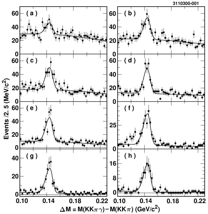
FIG. 1.: Fits to the $\Delta M=M(KK\pi\gamma)-M(KK\pi)$ distributions for candidate $D_{s}^{*+}$ events that are used to determine the $D_{s}^{*+}$ yields in the eight $x(D_{s}^{*+})$ ranges (a) $0.50-0.56$, (b) $0.56-0.62$, (c) $0.62-0.68$, (d) $0.68-0.74$, (e) $0.74-0.80$, (f) $0.80-0.86$, (g) $0.86-0.92$, and (h) $0.92-0.98$.

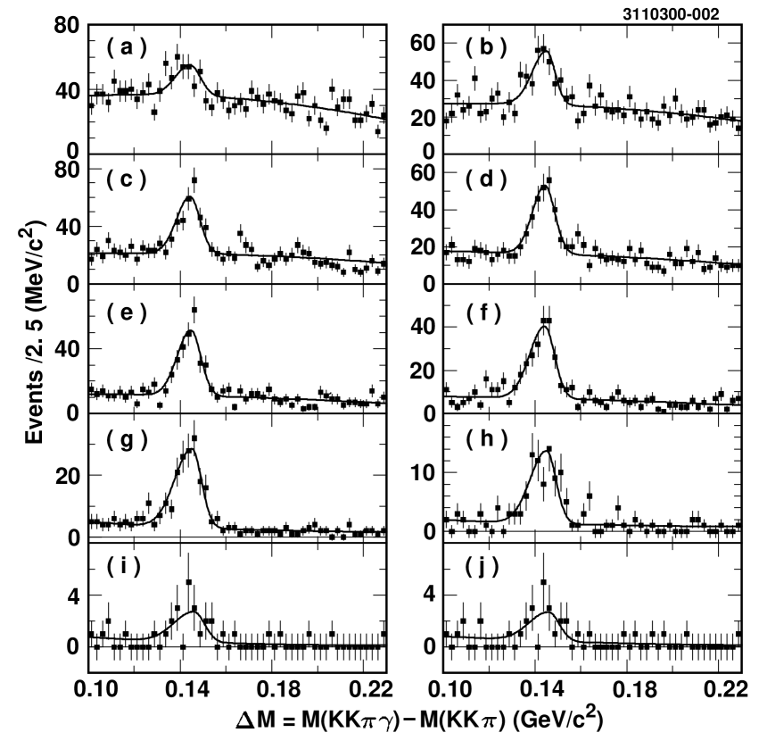
FIG. 2.: Fits to the $\Delta M=M(KK\pi\gamma)-M(KK\pi)$ distributions for candidate $D_{s}^{*+}$ events that are used to determine the $D_{s}^{*+}$ yields in the ten $x(D_{s}^{+})$ ranges (a) $0.44-0.50$, (b) $0.50-0.56$, (c) $0.56-0.62$, (d) $0.62-0.68$, (e) $0.68-0.74$, (f) $0.74-0.80$, (g) $0.80-0.86$, (h) $0.86-0.92$, (i) $0.92-0.98$, and (j) $0.92-1.00$.

The $M(KK\pi)$ distributions in data and the signal Monte Carlo sample are simultaneously fit to the sum of a double Gaussian with common mean for the $D_{s}^{+}$ signal, a Gaussian for the $D^{+}$ signal, two straight lines joined by a quadratic for the combinatoric background in data, and a first order Chebyshev polynomial for the small amount of background in the Monte Carlo sample. The fits to data used to determine the $D_{s}^{+}$ yields in the selected regions of $x(D_{s}^{+})$ are shown in Fig. 3.

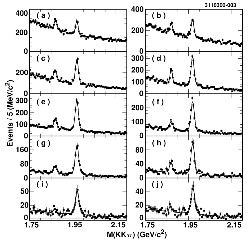
FIG. 3.: Fits to the $M(KK\pi)$ distributions for candidate $D_{s}^{+}$ events that are used to determine the $D_{s}^{+}$ yields in the ten $x(D_{s}^{+})$ ranges (a) $0.44-0.50$, (b) $0.50-0.56$, (c) $0.56-0.62$, (d) $0.62-0.68$, (e) $0.68-0.74$, (f) $0.74-0.80$, (g) $0.80-0.86$, (h) $0.86-0.92$, (i) $0.92-0.98$, and (j) $0.92-1.00$.

IV Efficiencies

The $D_{s}^{+}$ and $D_{s}^{*+}$ detection efficiencies are estimated using a sample of Monte Carlo events that contains signal as well as background events and is independent of the signal Monte Carlo sample used in the fitting procedure. The $D_{s}^{*+}$ efficiency values in the $x(D_{s}^{*+})$ regions are listed in Table I, while the $D_{s}^{+}$ and $D_{s}^{*+}$ efficiencies in the $x(D_{s}^{+})$ regions are listed in Table II.

$x(D_{s}^{*+})$ region	$D_{s}^{*+}$ Efficiency
0.50 - 0.56	$0.172\pm 0.008$
0.56 - 0.62	$0.175\pm 0.006$
0.62 - 0.68	$0.178\pm 0.005$
0.68 - 0.74	$0.181\pm 0.004$
0.74 - 0.80	$0.184\pm 0.004$
0.80 - 0.86	$0.187\pm 0.005$
0.86 - 0.92	$0.190\pm 0.006$
0.92 - 0.98	$0.193\pm 0.008$
(0.92 - 1.00)	($0.194\pm 0.008$)

TABLE I.: $D_{s}^{*+}$ detection efficiencies in the specified regions of $x(D_{s}^{*+})$, where the efficiency has been smoothed using a fit to the raw efficiency spectrum with a first order Chebyshev polynomial. The values that are in parentheses are used only for the calculation of the total $D_{s}^{*+}$ yield and cross-section for $x(D_{s}^{*+})>0.5$.

$x(D_{s}^{+})$ region	$D_{s}^{+}$ Efficiency	$D_{s}^{*+}$ Efficiency
0.44 - 0.50	$0.366\pm 0.010$	$0.180\pm 0.009$
0.50 - 0.56	$0.369\pm 0.008$	$0.179\pm 0.007$
0.56 - 0.62	$0.373\pm 0.007$	$0.178\pm 0.006$
0.62 - 0.68	$0.376\pm 0.005$	$0.177\pm 0.005$
0.68 - 0.74	$0.379\pm 0.005$	$0.176\pm 0.004$
0.74 - 0.80	$0.382\pm 0.005$	$0.175\pm 0.005$
0.80 - 0.86	$0.386\pm 0.007$	$0.174\pm 0.006$
0.86 - 0.92	$0.389\pm 0.008$	$0.140\pm 0.027$
0.92 - 0.98	$0.392\pm 0.010$	$0.248\pm 0.107$
(0.92 - 1.00)	($0.393\pm 0.011$)	($0.248\pm 0.106$)

TABLE II.: $D_{s}^{+}$ and $D_{s}^{*+}$ detection efficiencies in the specified regions of $x(D_{s})$ where the efficiency has been smoothed using a fit to the raw efficiency spectrum with a first order Chebyshev polynomial. The values that are in parentheses are used for the calculation of $P_{V}(D_{s})$. The $D_{s}^{*+}$ efficiency values with $x(D_{s}^{+})>0.86$ are excluded from the smoothing process because they are not expected to be modeled by the same function used for $x(D_{s}^{+})<0.86$.

For the $D_{s}^{*+}$ production study, the efficiency for each $x(D_{s}^{*+})$ bin is measured using the fitting procedure described above. The binned raw efficiency values within the range $0.50<x(D_{s}^{*+})<0.98$ are fit with a first order Chebyshev polynomial to provide a smoothly varying efficiency as a function of $x(D_{s}^{*+})$. The smoothed efficiency value at the center of each $x(D_{s}^{*+})$ region is used to calculate the efficiency corrected $D_{s}^{*+}$ yield and cross-section.

For the $D_{s}^{+}$ fragmentation study, the $D_{s}^{+}$ and $D_{s}^{*+}$ efficiencies are measured in each $x(D_{s}^{+})$ bin using the fitting procedure described above. The binned raw $D_{s}^{+}$ efficiencies within the range $0.44<x(D_{s}^{+})<0.98$ are fit with a first-order Chebyshev and the smoothed efficiency values are used to calculate the efficiency corrected $D_{s}^{+}$ yields. The binned raw $D_{s}^{*+}$ efficiencies with $0.44<x(D_{s}^{+})<0.86$ are fit with a first-order Chebyshev polynomial but the efficiencies in the region $x(D_{s}^{+})>0.86$ are excluded from the fit because of expected efficiency loss due to the larger proportion of photons in that region with energies less than 100 MeV. The smoothed efficiency values are used to calculate the efficiency corrected $D_{s}^{*+}$ yields for $x(D_{s}^{+})<0.86$, while the raw efficiency values are used for $x(D_{s}^{+})>0.86$.

V Results

The $D_{s}^{*+}$ yields, efficiency corrected yields and cross-sections in the eight $x(D_{s}^{*+})$ regions are all listed in Table III. These same quantities for $D_{s}^{+}$ and $D_{s}^{*+}$ in the nine $x(D_{s}^{+})$ regions are listed in Tables IV and V, respectively. The calculated primary $D_{s}^{+}$ yields and cross-sections are presented in Table VI.

	Measured	Efficiency Corrected
$x(D_{s}^{*+})$ region	$D_{s}^{*+}$ Yield	$D_{s}^{*+}$ Yield	${\cal B}\cdot\sigma(D_{s}^{*+})$(pb)
0.50 - 0.56	$84\pm 18$	$488\pm 116$	$0.10\pm 0.02$
0.56 - 0.62	$159\pm 19$	$911\pm 138$	$0.19\pm 0.03$
0.62 - 0.68	$173\pm 19$	$972\pm 137$	$0.21\pm 0.03$
0.68 - 0.74	$183\pm 17$	$1014\pm 131$	$0.21\pm 0.03$
0.74 - 0.80	$202\pm 17$	$1095\pm 135$	$0.23\pm 0.03$
0.80 - 0.86	$172\pm 16$	$918\pm 117$	$0.19\pm 0.02$
0.86 - 0.92	$148\pm 13$	$778\pm 100$	$0.16\pm 0.02$
0.92 - 0.98	$84\pm 10$	$434\pm 65$	$0.09\pm 0.01$
(0.92 - 1.00)	($99\pm 11$)	($511\pm 74$)	($0.11\pm 0.02$)
0.50 - 1.00	$1219\pm 47$	$6687\pm 260\pm 497$	$1.42\pm 0.06\pm 0.11$

TABLE III.: $D_{s}^{*+}$ yields, efficiency corrected yields and cross sections in the specified regions of $x(D_{s}^{*+})$, where ${\cal B}\equiv{\cal B}(D_{s}^{*+}\to D_{s}^{+}\gamma){\cal B}(D_{s}^{+}\to\phi\pi^{+}){\cal B}(\phi\to K^{+}K^{-})$. The uncertainty in the efficiency corrected yields and cross-sections includes both statistical and systematic error. When two errors are presented, the first is statistical while the second is systematic.

	Measured	Efficiency Corrected
$x(D_{s}^{+})$ region	$D_{s}^{+}$ Yield	$D_{s}^{+}$ Yield	${\cal B}\cdot\sigma(D_{s}^{+})$(pb)
0.44 - 0.50	$546\pm 43$	$1491\pm 140$	$0.32\pm 0.03$
0.50 - 0.56	$663\pm 40$	$1795\pm 139$	$0.38\pm 0.03$
0.56 - 0.62	$933\pm 40$	$2504\pm 160$	$0.53\pm 0.03$
0.62 - 0.68	$1019\pm 38$	$2712\pm 160$	$0.57\pm 0.03$
0.68 - 0.74	$1080\pm 40$	$2847\pm 166$	$0.60\pm 0.04$
0.74 - 0.80	$925\pm 36$	$2418\pm 145$	$0.51\pm 0.03$
0.80 - 0.86	$759\pm 31$	$1968\pm 122$	$0.42\pm 0.03$
0.86 - 0.92	$404\pm 24$	$1038\pm 79$	$0.22\pm 0.02$
0.92 - 0.98	$170\pm 14$	$433\pm 42$	$0.09\pm 0.01$
(0.92 - 1.00)	($187\pm 17$)	($476\pm 50$)	($0.10\pm 0.01$)
0.44 - 1.00	$6516\pm 106$	$17250\pm 281\pm 528$	$3.65\pm 0.06\pm 0.11$

TABLE IV.: $D_{s}^{+}$ yields and cross-sections in the specified regions of $x(D_{s}^{+})$, where ${\cal B}\equiv{\cal B}(D_{s}^{+}\to\phi\pi^{+}){\cal B}(\phi\to K^{+}K^{-})$. The $D_{s}^{+}$ yields are efficiency corrected using smoothed efficiency values. The uncertainty in the efficiency corrected yields and cross-sections includes both statistical and systematic error. When two errors are presented, the first is statistical while the second is systematic.

	Measured	Efficiency Corrected
$x(D_{s}^{+})$ region	$D_{s}^{*+}$ Yield	$D_{s}^{*+}$ Yield	${\cal B}\cdot\sigma(D_{s}^{*+})$(pb)
0.44 - 0.50	$104\pm 21$	$577\pm 129$	$0.13\pm 0.03$
0.50 - 0.56	$145\pm 19$	$808\pm 133$	$0.18\pm 0.03$
0.56 - 0.62	$200\pm 20$	$1122\pm 152$	$0.25\pm 0.03$
0.62 - 0.68	$181\pm 18$	$1020\pm 138$	$0.23\pm 0.03$
0.68 - 0.74	$208\pm 18$	$1180\pm 148$	$0.27\pm 0.03$
0.74 - 0.80	$182\pm 16$	$1040\pm 133$	$0.23\pm 0.03$
0.80 - 0.86	$149\pm 14$	$852\pm 113$	$0.19\pm 0.03$
0.86 - 0.92	$70\pm 9$	$501\pm 202$	$0.11\pm 0.05$
0.92 - 0.98	$16\pm 5$	$63\pm 39$	$0.01\pm 0.01$
(0.92 - 1.00)	($15\pm 5$)	($60\pm 37$)	($0.01\pm 0.01$)
0.44 - 1.00	$1253\pm 49$	$7160\pm 279\pm 550$	$1.61\pm 0.06\pm 0.11$

TABLE V.: $D_{s}^{*+}$ yields and cross-sections in the specified regions of $x(D_{s}^{+})$, where ${\cal B}\equiv{\cal B}(D_{s}^{+}\to\phi\pi^{+}){\cal B}(\phi\to K^{+}K^{-})$. The first seven $D_{s}^{*+}$ yields are efficiency corrected using the smoothed efficiency values while the efficiencies for $x(D_{s}^{+})>0.86$ are corrected using the raw efficiency values. The uncertainty in the efficiency corrected yields and cross-sections includes both statistical and systematic error. When two errors are presented the first is statistical while the second systematic.

$x(D_{s}^{+})$ region	Primary $D_{s}^{+}$ Yield	Primary ${\cal B}\cdot\sigma(D_{s}^{+})$(pb)
0.44 - 0.50	$878\pm 197$	$0.19\pm 0.04$
0.50 - 0.56	$937\pm 200$	$0.20\pm 0.04$
0.56 - 0.62	$1313\pm 230$	$0.28\pm 0.05$
0.62 - 0.68	$1630\pm 219$	$0.35\pm 0.05$
0.68 - 0.74	$1594\pm 231$	$0.34\pm 0.05$
0.74 - 0.80	$1315\pm 204$	$0.28\pm 0.04$
0.80 - 0.86	$1063\pm 173$	$0.23\pm 0.04$
0.86 - 0.92	$506\pm 229$	$0.11\pm 0.05$
0.92 - 0.98	$370\pm 57$	$0.08\pm 0.01$
(0.92 - 1.00)	($417\pm 64)$	($0.09\pm 0.01$)
0.44 - 1.00	$9652\pm 408\pm 760$	$2.05\pm 0.09\pm 0.16$

TABLE VI.: Calculated primary $D_{s}^{+}$ yields and cross sections in the specified regions of $x(D_{s}^{+})$. The cross-section is presented as ${\cal B}\cdot\sigma$ where ${\cal B}\equiv{\cal B}(D_{s}^{+}\to\phi\pi^{+}){\cal B}(\phi\to K^{+}K^{-})$. The errors in each $x(D_{s}^{+})$ bin include both statistical and systematic uncertainty. When two errors are presented, the first is statistical while the second is systematic.

By summing the efficiency corrected $D_{s}^{*+}$ and primary $D_{s}^{+}$ yields listed in Tables III and VI, respectively, Eq. (1) could be used to calculate $P_{V}$ for $x(D_{s}^{(*)+})>0.5$. However, the uncertainties in the $D_{s}^{*+}$ yields are essentially counted twice due to the subtraction used to calculate the primary $D_{s}^{+}$ yields. $P_{V}$ can however be calculated in a way that avoids this subtraction. Since all observed $D_{s}^{*+}$ mesons are assumed to be primary, all observed $D_{s}^{+}$ mesons are assumed to be either primary or $D_{s}^{*+}$ daughters, and all $D_{s}^{*+}$ are expected to decay to a $D_{s}^{+}$, Eq. (1) can be rewritten as

$$P_{V}=\frac{T(D_{s}^{*+})}{T(D_{s}^{+})}~{},$$ (6)

where $T(M)$ is the total number of $M$ mesons in the CLEO II data sample. In terms of the quantities measured using the decay modes chosen for this analysis,

$$P_{V}=\frac{n(D_{s}^{*+})}{n(D_{s}^{+}){\cal B}(D_{s}^{*+}\to D_{s}^{+}\gamma)}~{},$$ (7)

where $n(M)$ is the efficiency corrected yield of $M$ mesons in a particular $x(D_{s}^{+})$ region. Using this method, $P_{V}(x(D_{s}^{+})>0.44){\cal B}(D_{s}^{*+}\to D_{s}^{+}\gamma)=0.42\pm 0.02$. Using the value ${\cal B}(D_{s}^{*+}\to D_{s}^{+}\gamma)=(94.2\pm 2.5)\%$ [6] leads to $P_{V}(x(D_{s})>0.44)=0.44\pm 0.02(stat.)\pm 0.01(br.)$.

VI Systematic Uncertainty

The systematic error for the total $D_{s}^{+}$ and $D_{s}^{*+}$ yields is determined by varying the selection and fitting procedures as described below and taking the variance in the total yield as the estimate of the error. The variance is also determined on a bin-by-bin basis and the average percentage variance in the individual bins is taken as the estimated systematic uncertainty for all bins. The uncertainties in the $D_{s}^{*+}$ yields for the range $0.86<x(D_{s}^{+})<1.0$ are averaged separately since those values are not smoothed and the errors are quite large due to the limited number of $D_{s}^{*+}$ events in that region. Systematic uncertainties on the various yields are listed in Tables VII and VIII.

Variation	Percent Variance
$D_{s}^{+}$ peak in $M(KK\pi)$ fit with Gaussian	2%(3%)
$D^{+}$ peak in $M(KK\pi)$ fit with double Gaussian	1%(1%)
$D_{s}^{+}$ background fit with quadratic	2%(3%)

TABLE VII.: Percent variance in total(bin-by-bin) $D_{s}^{+}$ yields compared to the nominal yields due to the listed sources of systematic error.

Variation	Percent Variance
15 MeV/$c^{2}$ wide $M(KK\pi)$ signal region	1%(3%)
25 MeV/$c^{2}$ wide $M(KK\pi)$ signal region	1%(2%)
$\Delta M$ peak fit with Gaussian	1%(1%)
$\Delta M$ peak fit with double bifurcated Gaussian	2%(3%)
$\cos\theta_{s}<0.6$	6%(6%)
$E(\gamma)>90,110$ MeV	2%(3%)
Uncertainty in $\gamma$ efficiency from ${\cal B}(\eta\to\gamma\gamma)/{\cal B}(\eta\to 3\pi^{0})$ study	3%(3%)

TABLE VIII.: Percent variance in total(bin-by-bin) $D_{s}^{*+}$ yields compared to the nominal yields due to the listed sources of systematic error.

The acceptance angles for showers implicitly alter the acceptance of tracks since there is a high degree of correlation between the flight directions of the $D_{s}^{+}$ and the photon in the detector. There is also a correlation between the photon energy and the decay angle of the $D_{s}^{*+}$. Varying the shower acceptance angles to $|\cos\theta_{s}|<0.5$ changes the total $D_{s}^{*+}$ yields and the bin-by-bin yields by approximately 6%, while changing the minimum shower energy to either 90 MeV or 110 MeV changes the total $D_{s}^{*+}$ yield by approximately 2% and the bin-by-bin yields by approximately 3%. A 3% overall systematic uncertainty in photon reconstruction has been estimated by comparing the world average value of ${\cal B}(\eta\to\gamma\gamma)/{\cal B}(\eta-3\pi^{0})$ [1] with the relative yields of $\eta\to\gamma\gamma$ and $\eta\to 3\pi^{0}$ in data and Monte Carlo.

Additional uncertainty exists because of differences in invariant mass distributions between data and Monte Carlo and possible inadequacies of the fitting functions used to determine the yields. This uncertainty is estimated by altering the fitting shapes used to obtain the $D_{s}^{+}$ and $D_{s}^{*+}$ yields. Varying the fitting technique for the $M(KK\pi)$ projections by e.g. using a Gaussian for the $D_{s}^{+}$ signal peak, a double Gaussian with common mean for the $D^{+}$ signal peak, or a second-order polynomial for the background alters the total $D_{s}^{+}$ yield by approximately 3% and the bin-by-bin yields by approximately 4%. Using a single Gaussian or double bifurcated Gaussian with a common mean for the peak in the $\Delta M$ distribution alters the total $D_{s}^{*+}$ yield by approximately 2% and the bin-by-bin yields by approximately 3%.

There is also an uncertainty related to the requirement that $M(KK\pi)$ be within 20 MeV/$c^{2}$ of its nominal value. Widening this requirement to 25 MeV/$c^{2}$ and narrowing it to 15 MeV/$c^{2}$ has resulted in an approximate 2% error in the total $D_{s}^{*+}$ yield and an approximate 4% error in the bin-by-bin yields.

The uncertainties in the efficiency values shown in Tables I and II vary for each region of $x(D_{s}^{+})$ and $x(D_{s}^{*+})$ due to limited Monte Carlo statistics and the smoothing process. For instance, the errors in the smoothed efficiency values near the limits of the $x$ region studied are higher than those in the middle of the region due to the uncertainty in the slope of the function used in the smoothing process. The errors in the efficiency contribute to the systematic uncertainty on a bin-by-bin basis and the percentage errors are added in quadrature for the determination of the percentage error for the total yields.

All of the individual systematic uncertainties associated with a given yield are added together in quadrature with the percentage error in the efficiency to determine the total systematic uncertainty in the $D_{s}^{+}$ and $D_{s}^{*+}$ yields. These systematic uncertainties are already included in the errors in the yields in Tables III, IV, V and VI. After including the total systematic uncertainty, $P_{V}(x(D_{s}^{+})>0.44)=0.44\pm 0.02(stat.)\pm 0.03(syst.)\pm 0.01(br.)$.

VII Discussion of Results

The momentum distributions of hadrons created in the fragmentation process are commonly modeled with either the Andersson et al. symmetric fragmentation function [7] or the Peterson et al. fragmentation function [8]. Both of these functions depend upon $z=\frac{E_{h}+p_{\parallel}}{E+p}$, where $E_{h}$ is the energy of the hadron, $p_{\parallel}$ is the hadron momentum parallel to $p$, the momentum of the primary quark from the production process, and $E$ is the energy of the primary quark. The Andersson function is

$$f(z)\propto z^{-1}(1-z)^{a}\exp(-b\ m_{\bot}^{2}/z)~{},$$ (8)

where $a$ and $b$ are free parameters, $m_{\bot}=\sqrt{m_{q}^{2}+p_{\bot}^{2}}$, $m_{q}$ is the mass of the primary quark and $p_{\bot}$ is the hadron momentum perpendicular to $p$. The Peterson function is

$$f(z)\propto\frac{1}{z[1-(1/z)-\epsilon_{P}/(1-z)]^{2}}~{},$$ (9)

where $\epsilon_{P}$ is the single free parameter.

To properly compare fragmentation models with data it is necessary to use the above functions in a full Monte Carlo simulation that incorporates photon radiation, gluon radiation and other effects. To facilitate comparison with other experimental results, $x$ is used as an approximation of $z$ and a binned $\chi^{2}$ fit to the data is performed using these two functions as shown in Figs. 4 and 5. Since the parameters $b$ and $m_{\bot}$ only appear in Eq. (8) as a product, the constraint $b=1$ has been used for the fit, thereby changing the interpretation of the value of $m_{\bot}$. The numerical results from the fits are listed in Table IX. The normalizations of these fits are not used to calculate a value of $P_{V}$ due to differences between $x$ and $z$ that are non-negligible in the low $D_{s}$ momentum regime.

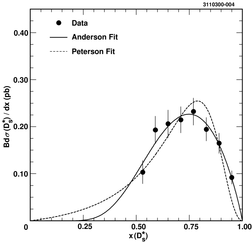
FIG. 4.: ${\cal B}\cdot\sigma(D_{s}^{*+})$ spectrum fit with the Andersson et al. and Peterson et al. fragmentation functions, where ${\cal B}\equiv{\cal B}(D_{s}^{*+}\to D_{s}^{+}\gamma){\cal B}(D_{s}^{+}\to\phi\pi^{+}){\cal B}(\phi\to K^{+}K^{-})$.

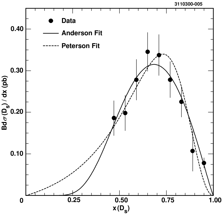
FIG. 5.: Primary ${\cal B}\cdot\sigma(D_{s}^{+})$ spectrum fit with the Andersson et al. and Peterson et al. fragmentation functions, where ${\cal B}\equiv{\cal B}(D_{s}^{+}\to\phi\pi^{+}){\cal B}(\phi\to K^{+}K^{-})$.

	Fit Results	$\chi^{2}$/d.o.f.
Andersson:
$D_{s}^{*+}$:	$a=0.9\pm 0.2$, $m_{\bot}=1.7\pm 0.1$	1.9/5
$D_{s}^{+}$:	$a=1.1\pm 0.2$, $m_{\bot}=1.5\pm 0.1$	3.2/6
Peterson:
$D_{s}^{*+}$:	$\epsilon_{P}=0.056\pm 0.008$	20.5/6
$D_{s}^{+}$:	$\epsilon_{P}=0.10\pm 0.02$	17.4/7

TABLE IX.: Results of fits to the $D_{s}^{*+}$ and $D_{s}^{+}$ spectra in $x(D_{s}^{*+})$ and $x(D_{s}^{+})$, respectively, with the Anderson et al. and Peterson et al. analytical fragmentation functions.

The fragmentation spectra for charm mesons has been studied previously by the CLEO collaboration[9] and input parameters for the Andersson et al. model were determined using measured fragmentation distributions for $D^{*+}$, $D^{0}$, $D^{+}$, $D_{s}$ and $\Lambda_{c}$. A comparison of the data presented here with a Monte Carlo distribution using the parameters determined in that study, $a=0.60$ and $b=0.52$, is shown in Figure 6. The use of these values as input parameters for charm fragmentation into $D_{s}$ mesons clearly result in a momentum distribution that is too soft, which is not surprising since P-wave charm meson decays to $D^{*+}$, $D^{0}$ and $D^{+}$ were not excluded in the prior study.

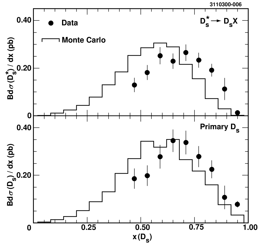
FIG. 6.: ${\cal B}\cdot\sigma(D_{s}^{*+})$ and ${\cal B}\cdot\sigma(D_{s}^{+})$ for primary $D_{s}$ compared to the Monte Carlo production spectrum using the Andersson et al. fragmentation function parameters $a=0.60$ and $b=0.52$ [9], where ${\cal B}\equiv{\cal B}(D_{s}^{+}\to\phi\pi^{+}){\cal B}(\phi\to K^{+}K^{-})$.

High levels of combinatoric background at low values of $x(D_{s}^{+})$ prohibit a good measurement of $P_{V}$ for the full range of allowed $D_{s}^{+}$ momenta. Based on Monte Carlo simulations and the data presented, approximately $75-85\%$ of all $D_{s}^{*+}$ and $D_{s}^{+}$ are expected to have $x(D_{s}^{+})>0.44$ and the value of $P_{V}$ presented here is not expected to differ much from $P_{V}$(all $x$).

It is possible to make a model-dependent extrapolation of $P_{V}$(all $x$) using

$$P_{V}(x>0)=\frac{1}{1+\left(\frac{1}{P_{V}(x>0.44)}-1\right)\frac{Q_{V}}{Q_{P}}}~{},$$ (10)

where $Q_{V}$ is the percentage of $D_{s}^{*+}$ that decay to a $D_{s}^{+}$ with $x(D_{s}^{+})>0.44$ and $Q_{P}$ is the fraction of primary $D_{s}^{+}$ that have $x(D_{s}^{+})>0.44$. Since only about one fifth of either fragmentation spectra lies below $x(D_{s}^{+})=0.44$, and because both distributions approach zero smoothly as $x(D_{s}^{+})\to 0$, the ratio $Q_{V}/Q_{P}$ is expected to be close to unity and to only depend weakly upon the chosen fragmentation parameters.

Using the Andersson et al. model with the parameters $a=0.60$ and $b=0.52$ results in $Q_{V}=0.773$, $Q_{P}=0.795$, $Q_{V}/Q_{P}=0.972$, and from Eq. (10), $P_{V}$(all $x(D_{s}^{+}))=0.45\pm 0.05$. Changing the input parameters to provide a harder spectrum has a very small effect on $Q_{V}/Q_{P}$. A distribution created with $a=0.4$ and $b=0.9$, for example, provides a much improved representation of the data and results in $Q_{V}=0.860$, $Q_{P}=0.875$, $Q_{V}/Q_{P}=0.983$ and $P_{V}$(all $x(D_{s}^{+}))=0.45\pm 0.05$. This clearly shows that the dependence of the $P_{V}$ extrapolation on the choice of fragmentation parameters is indeed weak.

Based on the results of varying the input parameters for the two models, a systematic uncertainty of 3% is estimated for the model-dependent extrapolation resulting in a final extrapolated value of $P_{V}$(all $x(D_{s}^{+}))=0.45\pm 0.05$, which is significantly different than the expected result based on spin counting.

Other measurements of $P_{V}$ for charm and bottom mesons have been presented [10, 11, 12, 13, 14], but it is difficult to make direct comparisons between those results and the one presented here because of differences in methodology and center-of-mass energies in the other analyses. Nonetheless, measurements of $P_{V}(B)$ are generally close to the spin-counting expectation while measurements of $P_{V}(D)$ are well below that value as shown in Table X.

Collaboration	Result
ALEPH [10]	$P_{V}(D_{s})=0.60\pm 0.19$
ALEPH [10]	$P_{V}(D)=0.60\pm 0.05$
OPAL [11]	$P_{V}(D)=0.57\pm 0.06$
SLD [12]	$P_{V}(D)=0.57\pm 0.07$
L3 [13]	$P_{V}(B)=0.76\pm 0.10$
OPAL [14]	$P_{V}(B)=0.76\pm 0.09$

TABLE X.: Results of previous measurements of $P_{V}$ for heavy quark mesons at other experiments. All of these measurements used data samples collected at $Z^{0}$ resonance.

VIII Conclusion

In summary, studies of $D_{s}^{*+}$ and $D_{s}^{+}$ fragmentation in $e^{+}e^{-}$ annihilations at $\sqrt{s}=10.5$ GeV have been presented. $P_{V}(x(D_{s})>0.44)$ has been measured to be $0.44\pm 0.02(stat.)\pm 0.03(syst.)\pm 0.01(br.)$. When extrapolated to the entire available momentum region this measurement deviates significantly from $P_{V}=0.75$, the expected result based on simple spin counting.

IX Acknowledgements

We gratefully acknowledge the effort of the CESR staff in providing us with excellent luminosity and running conditions. J.R. Patterson and I.P.J. Shipsey thank the NYI program of the NSF, M. Selen thanks the PFF program of the NSF, M. Selen and H. Yamamoto thank the OJI program of DOE, J.R. Patterson, K. Honscheid, M. Selen and V. Sharma thank the A.P. Sloan Foundation, M. Selen and V. Sharma thank the Research Corporation, F. Blanc thanks the Swiss National Science Foundation, and H. Schwarthoff and E. von Toerne thank the Alexander von Humboldt Stiftung for support. This work was supported by the National Science Foundation, the U.S. Department of Energy, and the Natural Sciences and Engineering Research Council of Canada.

REFERENCES

- [1] Particle Data Group, C. Caso et al., Eur. Phys. J. C 3, 1 (1998).
- [2] CLEO Collaboration, G. Brandenburg et al., Phys. Rev. D 58,052003 (1998).
- [3] P.V. Chliapnikov, Phys. Lett. B 470, 263 (1999); A. F. Falk and M. E. Peskin, Phys. Rev. D 49, 3320 (1994); E. Braatan, K. Cheung, S. Fleming and T.C. Yuan, Phys. Rev. D 51 4819 (1995); F. Becattini, Z. Phys. C 69 485 (1996); Y. Pei, Z. Phys. C 72 39 (1996).
- [4] CLEO Collaboration, Y. Kubota et al., Nucl. Instrum. Methods Phys. Res., Sec. A 320, 66 (1992).
- [5] T. Sjöstrand, Comput. Phys. Commun. 82, 47 (1994); T. Sjöstrand and M. Bengston ibid 43, 367 (1987); T. Sjöstrand, ibid 39, 347 (1986).
- [6] CLEO Collaboration, J. Gronberg et al., Phys. Rev. Lett. 75, 3232 (1995).
- [7] B. Andersson et al., Z. Phys. C 20, 317 (1983).
- [8] C. Peterson et al., Phys. Rev. D 27, 105 (1983).
- [9] CLEO Collaboration, D. Bortoletto et al., Phys. Rev. D 37, 1719 (1988). 62, 1 (1994).
- [10] ALEPH Collaboration, R. Barate et al., Submitted to Eur. Phys. J. C, hep-ex/9909032.
- [11] OPAL Collaboration, K. Ackerstaff et al., Eur. Phys. J. C 5, 1 (1998).
- [12] SLD Collaboration, K. Abe et al., presented at International Europhysics Conference on High-Energy Physics (HEP97), Jerusalem, Israel, 1997, Report No. SLAC-PUB 7574.
- [13] L3 Collaboration, M. Acciarri et al., Phys. Lett. B 345, 589 (1995).
- [14] OPAL Collaboration, K. Ackerstaff et al., Z. Phys. C 74, 413 (1997). (1994). University, Baltimore, Maryland, 1995, hep-ph/9505365.