DETERMINATION OF THE QCD COUPLING $\alpha_{\rm s}$

Abstract

Theoretical basics and experimental determinations of the coupling parameter of the Strong Interaction, $\alpha_{\rm s}$, are reviewed. The world average value of $\alpha_{\rm s}$, expressed at the energy scale of the rest mass of the $\rm Z^{0}$ boson, is determined from analyses which are based on complete NNLO perturbative QCD. The result is $\alpha_{\rm s}(M_{\rm Z^{0}})=0.1184\pm 0.0031$. No significant deviations or systematic biases of subsamples of experimental results are found. From the observed energy dependence of $\alpha_{\rm s}$, which is in excellent agreement with the expectations of QCD, the number of colour degrees of freedom can be constrained to $N_{c}=3.03\pm 0.12$.

1 Preface

The coupling strength $\alpha_{\rm s}$ is the basic free parameter of Quantum Chromodynamics (QCD), the theory of the Strong Interaction [1] which is one of the four fundamental forces of nature. QCD describes the interaction of quarks through the exchange of an octet of massless vector gauge bosons, the gluons, using similar concepts as known from Quantum Electrodynamics, QED. QCD, however, is more complex than QED because quarks and gluons, the analogues to electrons and photons in QED, are not observed as free particles but are confined inside hadrons.

Confinement implies that the coupling strength $\alpha_{\rm s}$, the analogue to the fine structure constant $\alpha$ in QED, becomes large in the regime of large-distance or low-momentum transfer interactions. Conversely, quarks and gluons are probed to behave like free particles, for short time intervals, in high-energy or short-distance reactions; they are said to be “asymptotically free”, i.e. $\alpha_{\rm s}\ \rightarrow$ 0 for momentum transfers $Q\ \rightarrow\ \infty$.

Within QCD, the phenomenology of confinement and of asymptotic freedom is realized by introducing a new quantum number, called “colour charge”. Quarks carry one out of three different colour charges, while hadrons are colourless bound states of 3 quarks or 3 antiquarks (“baryons”), or of a quark and an anti-quark (“mesons”). Gluons, in contrast to photons which do not carry (electrical) charge by themselves, have two colour charges. This concept leads to the process of gluon self-interaction, which in turn, through the effect of gluon vacuum polarization, gives rise to asymptotic freedom, i.e. the decrease of $\alpha_{\rm s}$ with increasing momentum transfer.

As in the case of QED, QCD predicts the energy dependence of $\alpha_{\rm s}$, while the actual value of $\alpha_{\rm s}$, at a given energy or four momentum transfer scale $Q$, is not predicted but must be determined from experiment.

Determining $\alpha_{\rm s}$ at a specific energy scale $Q$ is therefore a fundamental measurement, to be compared with measurements of the electromagnetic coupling $\alpha$, of the elementary electric charge, or of the gravitational constant. Testing QCD as such, however, requires the measurement of $\alpha_{\rm s}$ at least at two different energy scales, and/or at different processes: one measurement fixes the free parameter and thus provides accurate predictions for the value of $\alpha_{\rm s}$ at other energy scales and/or at other processes.

In general, $\alpha_{\rm s}$ can be determined in dynamic particle reactions involving in- or outgoing quarks and gluons, which manifest themselves as hadrons. Examples of Feynman diagrams describing hadronic final states in deep inelastic lepton-nucleon scattering (DIS), electron-positron annihilation (${\rm e^{+}\rm e^{-}}$), hadron collisions and quarkonia decays are shown in figure 1.

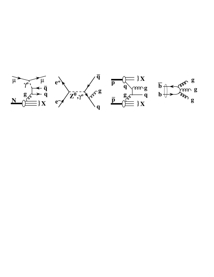
Figure 1: Examples of Feynman diagrams describing hadronic final states in processes which are used to measure $\alpha_{\rm s}$.

In this report, at the turn of the millennium, the current status of measurements of $\alpha_{\rm s}$ is reviewed. Theoretical basics of $\alpha_{\rm s}$ and QCD are given in Section 2. Measurements of $\alpha_{\rm s}$ from deep inelastic scattering, from ${\rm e^{+}\rm e^{-}}$ annihilation processes, from hadron colliders and from heavy quarkonia decays are discussed in Sections 3 to 6, respectively. A global summary of these results, a determination of the world average value of $\alpha_{\rm s}(M_{\rm Z^{0}})$ and quantitative studies of the energy dependence of $\alpha_{\rm s}$ are presented in Section 7. Section 8 concludes and gives an outlook to future developments.

2 QCD and $\alpha_{\rm s}$: basic theoretical predictions

The concepts of QCD are described in many text books and review articles, see e.g. references [2, 3]. A brief review of the basics of perturbative QCD and of the coupling strength $\alpha_{\rm s}$, like the concepts of renormalization, asymptotic freedom and confinement, the $\Lambda$ parameter, the treatment of quark masses and thresholds, perturbative predictions of physical observables and renormalization scale dependence, and of nonperturbative methods like lattice calculations will be presented in the following subsections.

2.1 Renormalization

In quantum field theories like QCD and QED, dimensionless physical quantities $\cal{R}$ can be expressed by a perturbation series in powers of the coupling parameter $\alpha_{\rm s}$ or $\alpha$, respectively. Consider $\cal{R}$ depending on $\alpha_{\rm s}$ and on a single energy scale $Q$. This scale shall be larger than any other relevant, dimensionful parameter such as quark masses. In the following, these masses are therefore set to zero.

When calculating $\cal{R}$ as a perturbation series in $\alpha_{\rm s}$, ultraviolet divergencies occur. Because $\cal{R}$ must retain physical values, these divergencies are removed by a procedure called “renormalization”. This introduces a second mass or energy scale, $\mu$, which represents the point at which the subtraction to remove the ultraviolet divergencies is actually performed. As a consequence of this procedure, $\cal{R}$ and $\alpha_{\rm s}$ become functions of the renormalization scale $\mu$. Since $\cal{R}$ is dimensionless, we assume that it only depends on the ratio $Q^{2}/\mu^{2}$ and on the renormalized coupling $\alpha_{\rm s}(\mu^{2})$:

$${\cal R}\equiv{\cal R}(Q^{2}/\mu^{2},\alpha_{\rm s});\ \alpha_{\rm s}\equiv\alpha_{\rm s}(\mu^{2}).$$

Because the choice of $\mu$ is arbitrary, however, $\cal{R}$ cannot depend on $\mu$, for a fixed value of the coupling, such that

$$\mu^{2}\frac{{\rm d}}{{\rm d}\mu^{2}}{\cal R}(Q^{2}/\mu^{2},\alpha_{\rm s})=\left(\mu^{2}\frac{\partial}{\partial\mu^{2}}+\mu^{2}\frac{\partial\alpha_{\rm s}}{\partial\mu^{2}}\frac{\partial}{\partial\alpha_{\rm s}}\right){\cal R}=^{\hskip-5.0pt!}\ 0\ ,$$ (1)

where the convention of multiplying the whole equation with $\mu^{2}$ is applied in order to keep the expression dimensionless. Equation 1 implies that any explicit dependence of $\cal{R}$ on $\mu$ must be cancelled by an appropriate $\mu$-dependence of $\alpha_{\rm s}$. It would therefore be natural to identify the renormalization scale with the physical energy scale of the process, $\mu^{2}=Q^{2}$, eliminating the uncomfortable presence of a second and unspecified scale. In this case, $\alpha_{\rm s}$ transforms to the “running coupling constant” $\alpha_{\rm s}(Q^{2})$, and the energy dependence of $\cal{R}$ enters only through the energy dependence of $\alpha_{\rm s}(Q^{2})$.

2.2 $\alpha_{\rm s}$ and its energy dependence

While QCD does not predict the actual size of $\alpha_{\rm s}$ at a particular energy scale, its energy dependence is precisely determined. If the renormalized coupling $\alpha_{\rm s}(\mu^{2})$ can be fixed (i.e. measured) at a given scale $\mu^{2}$, QCD definitely predicts the size of $\alpha_{\rm s}$ at any other energy scale $Q^{2}$ through the renormalization group equation

$$Q^{2}\frac{\partial\alpha_{\rm s}(Q^{2})}{\partial Q^{2}}=\beta\left(\alpha_{\rm s}(Q^{2})\right)\ .$$ (2)

The perturbative expansion of the $\beta$ function, including higher order loop corrections to the bare vertices of the theory, is calculated to complete 4-loop approximation [4]:

$$\beta(\alpha_{\rm s}(Q^{2}))=-\beta_{0}\alpha_{\rm s}^{2}(Q^{2})-\beta_{1}\alpha_{\rm s}^{3}(Q^{2})-\beta_{2}\alpha_{\rm s}^{4}(Q^{2})-\beta_{3}\alpha_{\rm s}^{5}(Q^{2})+{\cal O}(\alpha_{\rm s}^{6})\ ,$$ (3)

where

$$\beta_{0} = \frac{33-2N_{f}}{12\pi}\ ,$$

$$\beta_{1} = \frac{153-19N_{f}}{24\pi^{2}}\ ,$$

$$\beta_{2} = \frac{77139-15099N_{f}+325N_{f}^{2}}{3456\pi^{3}}\ ,$$

$$\beta_{3} \approx \frac{29243-6946.3N_{f}+405.089N_{f}^{2}+1.49931N_{f}^{3}}{256\pi^{4}}\ ,$$ (4)

and $N_{f}$ is the number of active quark flavours at the energy scale $Q$. The numerical constants in equation 2.2 are functions of the group constants $C_{A}$ and $C_{F}$, which for QCD — exhibiting $SU(3)$ symmetry — have values of $C_{A}=3$ and $C_{F}=4/3$ (see e.g. [2] for more details). $\beta_{0}$ and $\beta_{1}$ are independent of the renormalization scheme, while all higher order $\beta$ coefficients are scheme dependent.

2.3 Asymptotic freedom and confinement

A solution of equation 3 in 1-loop approximation, i.e. neglecting $\beta_{1}$ and higher order terms, is

$$\alpha_{\rm s}(Q^{2})=\frac{\alpha_{\rm s}(\mu^{2})}{1+\alpha_{\rm s}(\mu^{2})\beta_{0}\ln{\frac{Q^{2}}{\mu^{2}}}}\ .$$ (5)

Apart from giving a relation between $\alpha_{\rm s}(Q^{2})$ and $\alpha_{\rm s}(\mu^{2})$, equation 5 also demonstrates the property of asymptotic freedom: if $Q^{2}$ becomes large and $\beta_{0}$ is positive, i.e. if $N_{f}<17$, $\alpha_{\rm s}(Q^{2})$ will decrease to zero.

Likewise, equation 5 indicates that $\alpha_{\rm s}(Q^{2})$ grows to large values and actually diverges to infinity at small $Q^{2}$: for instance, with $\alpha_{\rm s}(\mu^{2}\equiv M^{2}_{\rm Z^{0}})=0.12$ and for typical values of $N_{f}=2\ ...\ 5$, $\alpha_{\rm s}(Q^{2})$ exceeds unity for $Q^{2}\leq\cal{O}\rm{(100~{}MeV~{}...~{}1~{}GeV)}$. Clearly, this is the region where perturbative expansions in $\alpha_{\rm s}$ are not meaningful anymore, and we may regard energy scales of $\mu^{2}$ and $Q^{2}$ below the order of 1 GeV as the nonperturbative region where confinement sets in, and where equations 3 and 5 cannot be applied.

Including $\beta_{1}$ and higher order terms, similar but more complicated relations for $\alpha_{\rm s}(Q^{2})$, as a function of $\alpha_{\rm s}(\mu^{2})$ and of $\ln{\frac{Q^{2}}{\mu^{2}}}$ as in equation 5, emerge. They can be solved numerically, such that for a given value of $\alpha_{\rm s}(\mu^{2})$, choosing a suitable reference scale like the mass of the $\rm Z^{0}$ boson, $\mu=M_{\rm Z^{0}}$, $\alpha_{\rm s}(Q^{2})$ can be accurately determined at any energy scale $Q^{2}\geq 1~{}\rm{GeV}^{2}$.

2.4 The $\Lambda$ parameter

Alternatively, as another parametrization of $\alpha_{\rm s}(Q^{2})$, a parameter called $\Lambda$ is introduced as a constant of integration of the $\beta$-function, such that, in leading order,

$$\alpha_{\rm s}(Q^{2})=\frac{1}{\beta_{0}\ln(Q^{2}/\Lambda^{2})}\ .$$ (6)

Equations 5 and 6 are equivalent with each other if

$$\Lambda^{2}=\frac{\mu^{2}}{e^{1/\left(\beta_{0}\alpha_{\rm s}(\mu^{2})\right)}}\ .$$

Hence, $\alpha_{\rm s}(\mu^{2})$ is replaced by a suitable choice of the $\Lambda$ parameter, which technically is identical to the energy scale $Q$ where $\alpha_{\rm s}(Q^{2})$ diverges to infinity, $\alpha_{\rm s}(Q^{2})\rightarrow\infty$ for $Q^{2}\rightarrow\Lambda^{2}$. To give a numerical example, $\Lambda\approx 0.1$ GeV for $\alpha_{\rm s}(M_{\rm Z^{0}}\equiv 91.2\ \rm{GeV})=0.12$ and $N_{f}$ = 5.

The parametrization of the running coupling $\alpha_{\rm s}(Q^{2})$ with $\Lambda$ instead of $\alpha_{\rm s}(\mu^{2})$ has become a common standard, see e.g. reference [5], and will also be adapted in this review. While being a convenient and well-used choice, however, this parametrization has several shortcomings which the user should be aware of.

First, requiring that $\alpha_{\rm s}(Q^{2})$ must be continuous when crossing a quark threshold, $\Lambda$ actually depends on the number of active quark flavours. Secondly, $\Lambda$ depends on the renormalization scheme, see e.g. reference [6]. In this review, the so-called “modified minimal subtraction scheme” ($\overline{\mbox{MS}}$) [7] will be adopted, which also has become a common standard [5]. $\Lambda$ will therefore be labelled $\Lambda_{\overline{\mbox{\scriptsize MS}}}^{(N_{f})}$ to indicate these peculiarities.

In complete 4-loop approximation and using the $\Lambda$-parametrization, the running coupling is thus given [8] by

$$\alpha_{\rm s}(Q^{2}) = \frac{1}{\beta_{0}L}-\frac{1}{\beta_{0}^{3}L^{2}}\beta_{1}\ln L$$

$$+ \frac{1}{\beta_{0}^{3}L^{3}}\left(\frac{\beta_{1}^{2}}{\beta_{0}^{2}}\left(\ln^{2}L-\ln L-1\right)+\frac{\beta_{2}}{\beta_{0}}\right)$$

$$+ \frac{1}{\beta_{0}^{4}L^{4}}\left(\frac{\beta_{1}^{3}}{\beta_{0}^{3}}\left(-\ln^{3}L+\frac{5}{2}\ln^{2}L+2\ln L-\frac{1}{2}\right)-3\frac{\beta_{1}\beta_{2}}{\beta_{0}^{2}}\ln L+\frac{\beta_{3}}{2\beta_{0}}\right)$$

(7)

where $L=Q^{2}/\Lambda_{\overline{\mbox{\scriptsize MS}}}^{2}$. The first line of equation 2.4 includes the 1- and the 2-loop coefficients, the second line is the 3-loop and the third line is the 4-loop correction, respectively.

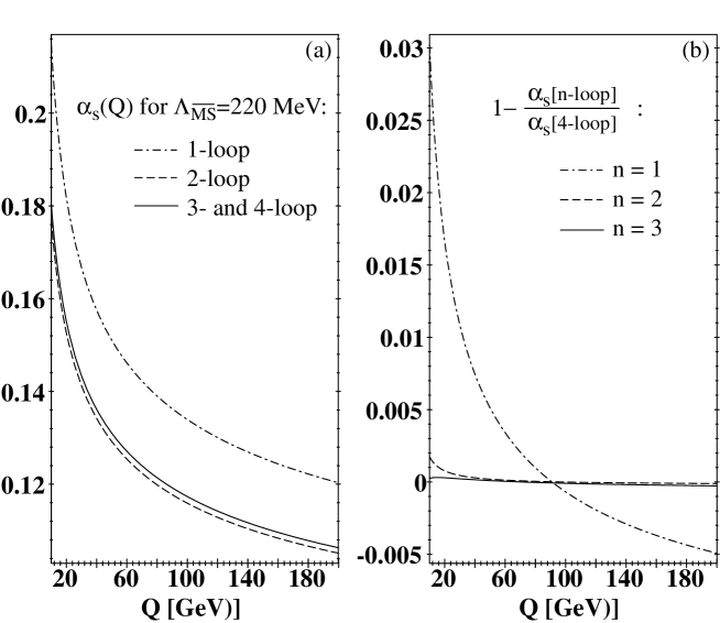
Figure 2: (a) The running of $\alpha_{\rm s}(Q)$, according to equation 2.4, in 1-, 2- and 3-loop approximation, for $N_{f}=5$ and with an identical value of $\Lambda_{\overline{\mbox{\scriptsize MS}}}=0.22$ GeV. The 4-loop prediction is indistinguishable from the 3-loop curve. (b) Fractional difference between the 4-loop and the 1-, 2- and 3-loop presentations of $\alpha_{\rm s}(Q)$, for $N_{f}=5$ and $\Lambda_{\overline{\mbox{\scriptsize MS}}}$ chosen such that, in each order, $\alpha_{\rm s}(M_{\rm Z^{0}})=0.119$.

The functional form of $\alpha_{\rm s}(Q)$, for the 1-, the 2- and the 3-loop approximation of equation 2.4, each with $\Lambda=0.220$ GeV, is shown in figure 2(a). As can be seen, there is an almost 15% decrease of $\alpha_{\rm s}$ when changing from 1-loop to 2-loop approximation, for the same value of $\Lambda$. The difference between the 2-loop and the 3-loop prediction is only about 1-2%, and is less than 0.01% between the 3-loop and the 4-loop presentation which cannot be resolved in the figure.

The fractional difference in the energy dependence of $\alpha_{\rm s}$, $\frac{(\alpha_{\rm s}^{(4-loop)}-\alpha_{\rm s}^{(n-loop)})}{\alpha_{\rm s}^{(4-loop)}}$, for $n$ = 1, 2 and 3, is presented in figure 2(b). Here, in contrast to figure 2(a), the values of $\Lambda_{\overline{\mbox{\scriptsize MS}}}$ were chosen such that $\alpha_{\rm s}(M_{\rm Z^{0}})=0.119$ in each order, i.e., $\Lambda_{\overline{\mbox{\scriptsize MS}}}=93$ MeV (1-loop), $\Lambda_{\overline{\mbox{\scriptsize MS}}}=239$ MeV (2-loop), and $\Lambda_{\overline{\mbox{\scriptsize MS}}}=220$ MeV (3- and 4-loop). Only the 1-loop approximation shows sizeable differences of up to several per cent, in the energy and parameter range chosen, while the 2- and 3-loop approximation already reproduce the energy dependence of the best, i.e. 4-loop, prediction quite accurately.

2.5 Quark masses and thresholds

So far in this discussion, finite quark masses $m_{q}$ were neglected, assuming that both the physical and the renormalization scales $Q^{2}$ and $\mu^{2}$, respectively, are larger than any other relevant energy or mass scale involved in the problem. This is, however, not entirely correct, since there are several QCD studies and $\alpha_{\rm s}$ determinations at energy scales around the charm- and bottom-quark masses of about 1.5 and 4.7 GeV, respectively.

Finite quark masses may have two major effects on actual QCD studies: Firstly, quark masses will alter the perturbative predictions of observables $\cal{R}$. While phase space effects which are introduced by massive quarks can often be studied using hadronization models and Monte Carlo simulation techniques, explicit quark mass corrections in higher than leading perturbative order are available only for jet production [9] and for total hadronic cross sections [10, 11] in ${\rm e^{+}\rm e^{-}}$ annihilation.

Secondly, any quark-mass dependence of $\cal{R}$ will add another term $\mu^{2}\frac{\partial m}{\partial\mu^{2}}\frac{\partial}{\partial m}{\cal R}$ to equation 1, which leads to energy-dependent, running quark masses, $m_{q}(Q^{2})$, in a similar way as the running coupling $\alpha_{\rm s}(Q^{2})$ was obtained, see e.g. reference [2].

In addition to these effects, $\alpha_{\rm s}$ indirectly also depends on the quark masses, through the dependence of the $\beta$ coefficients on the effective number of quarks flavours, $N_{f}$, with $m_{q}\ll\mu$. Constructing an effective theory for, say, ($N_{f}$-1) quark flavours which must be consistent with the $N_{f}$ quark flavours theory at the heavy quark threshold $\mu^{(N_{f})}\sim{\cal O}(m_{q})$, results in matching conditions for the $\alpha_{\rm s}$ values of the ($N_{f}$-1)- and the $N_{f}$-quark flavours theories [12].

In leading and in next-to-leading order, the matching condition is $\alpha_{\rm s}^{(N_{f}-1)}=\alpha_{\rm s}^{N_{f}}$. In higher orders and the $\overline{MS}$ scheme, however, nontrivial matching conditions apply [12, 13, 8]. Formally these are, if the energy evolution of $\alpha_{\rm s}$ is performed in $n^{th}$ order, of order ($n-1$).

The matching scale $\mu^{(N_{f})}$ can be chosen in terms of the (running) $\overline{MS}$ mass $m_{q}(\mu_{q})$, or of the constant, so-called pole mass $M_{q}$. For both cases, the relevant matching conditions in NNLO are given in [8]. These expressions have a particluarly simple form for the choice $\mu^{(N_{f})}=m_{q}(m_{q})$ or $\mu^{(N_{f})}=M_{q}$. In this report, the latter choice will be used to perform 3-loop matching at the heavy quark pole masses, in which case the matching condition reads, with $a=\alpha_{\rm s}^{(N_{f})}/\pi$ and $a^{\prime}=\alpha_{\rm s}^{(N_{f}-1)}/\pi$:

$$\frac{a^{\prime}}{a}=1+C_{2}\ a^{2}+C_{3}\ a^{3}\ ,$$ (8)

where $C_{2}=-0.291667$ and $C_{3}=-5.32389+(N_{f}-1)\cdot 0.26247$ [8].

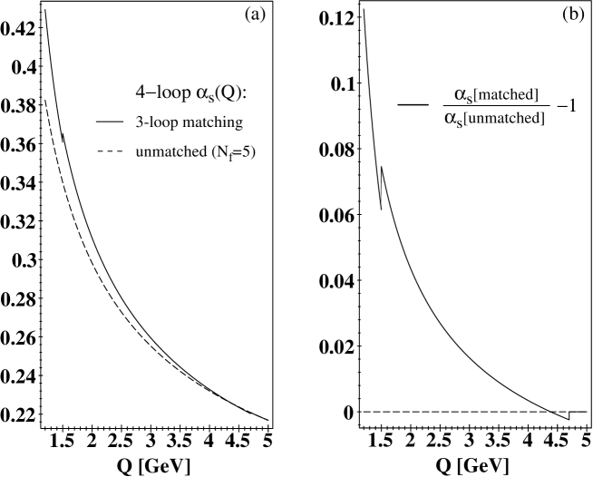
Figure 3: (a) 4-loop running of $\alpha_{\rm s}(Q)$ with 3-loop quark threshold matching according to equations 2.4 and 8, with $\Lambda_{\overline{\mbox{\scriptsize MS}}}^{(N_{f}=5)}$ = 220 MeV and charm- and bottom-quark thresholds at the pole masses, $\mu^{(N_{f}=4)}_{c}\equiv M_{c}=1.5$ GeV and $\mu^{(N_{f}=5)}_{b}\equiv M_{b}=4.7$ GeV (full line), compared with the unmatched 4-loop result (dashed line). (b) The fractional difference between the two curves in (a).

The 4-loop prediction for the running $\alpha_{\rm s}$, using equation 2.4 with $\Lambda_{\overline{\mbox{\scriptsize MS}}}^{(N_{f}=5)}$ = 220 MeV and 3-loop matching at the charm- and bottom-quark pole masses, $\mu^{(N_{f}=4)}_{c}=M_{c}=1.5$ GeV and $\mu^{(N_{f}=5)}_{b}=M_{b}=4.7$ GeV, is illustrated in figure 3a (full line). Small discontinuities at the quark thresholds can be seen, such that $\alpha_{\rm s}^{(N_{f}-1)}<\alpha_{\rm s}^{(N_{f})}$ by about 2 per mille at the bottom- and about 1 per cent at the charm-quark threshold. The corresponding values of $\Lambda_{\overline{\mbox{\scriptsize MS}}}$ are $\Lambda_{\overline{\mbox{\scriptsize MS}}}^{(N_{f}=4)}=305$ MeV and $\Lambda_{\overline{\mbox{\scriptsize MS}}}^{(N_{f}=3)}=346$ MeV [134]. Comparison with the 4-loop prediction, without applying threshold matching and for $\Lambda_{\overline{\mbox{\scriptsize MS}}}^{(N_{f}=5)}$ = 220 MeV and $N_{f}$ = 5 throughout (dashed line) demonstrates that, in spite of the discontinuities, the matched calculation shows a steeper rise towards smaller energies because of the larger values of $\Lambda_{\overline{\mbox{\scriptsize MS}}}^{(N_{f}=4)}$ and $\Lambda_{\overline{\mbox{\scriptsize MS}}}^{(N_{f}=3)}$.

The size of discontinuities and the changes of slopes are more clearly demonstrated in figure 3b, where the fractional difference between the two curves from figure 3a, i.e. between the matched and the unmatched calculation, is presented. Note that the step function of $\alpha_{\rm s}$ is not an effect which can be measured — the steps are artifacts of the truncated perturbation theory and the requirement that predictions for observables at energy scales around the matching point must be consistent and independent of the two possible choices of (neighbouring) values of $N_{f}$.

2.6 Perturbative predictions of physical quantities

In practice, $\alpha_{\rm s}$ is not an ‘observable’ by itself. Values of $\alpha_{\rm s}(\mu^{2})$ are determined from measurements of observables $\cal{R}$ for which perturbative predictions exist. These are usually given by a power series in $\alpha_{\rm s}(\mu^{2})$, like

$${\cal R}(Q^{2}) = P_{l}\sum_{n}R_{n}\alpha_{\rm s}^{n}$$ (9)

$$= P_{l}\left(R_{0}+R_{1}\alpha_{\rm s}(\mu^{2})+R_{2}(Q^{2}/\mu^{2})\alpha_{\rm s}^{2}(\mu^{2})+...\right)\ ,$$

where $R_{n}$ are the $n_{th}$ order coefficients of the perturbation series and $P_{l}R_{0}$ denotes the lowest-order value of $\cal R$.

For processes which involve gluons already in lowest order perturbation theory, $P_{l}$ itself may include (powers of) $\alpha_{\rm s}$. For instance, this happens in case of the hadronic decay width of heavy Quarkonia, $\Gamma(\Upsilon\rightarrow ggg\rightarrow\ hadrons)$ for which $P_{l}\propto\alpha_{\rm s}^{3}$. If no gluons are involved in lowest order, as e.g. in ${\rm e^{+}\rm e^{-}}\rightarrow\ q\overline{q}\rightarrow\ hadrons$ or in deep inelastic scattering processes, $P_{l}R_{0}$ is a constant and the usual choice is $P_{l}\equiv 1$. $R_{0}$ is called the lowest order coefficient and $R_{1}$ is the leading order (LO) coefficient. Following this naming convention, $R_{2}$ is the next-to-leading order (NLO) and $R_{3}$ is the next-to-next-to-leading order (NNLO) coefficient.

QCD calculations in NLO perturbation theory are available for many observables $\cal{R}$ in high energy particle reactions; calculations including the complete NNLO are available for some totally inclusive quantities, like the total hadronic cross section in ${\rm e^{+}\rm e^{-}}\rightarrow\ hadrons$, moments and sum rules of structure functions in deep inelastic scattering processes and the hadronic decay width of the $\tau$ lepton. The complicated nature of QCD, due to the process of gluon self-coupling and the resulting large number of Feynman diagrams in higher orders of perturbation theory, so far limited the number of QCD calculations in complete NNLO.

An alternative approach to calculating higher order corrections is based on the resummation of leading logarithms which arise from soft and collinear singularities in gluon emission [14]. In such a case, the effective expansion parameter is $\alpha_{\rm s}L^{2}$ rather than $\alpha_{\rm s}$, where $L=\ln(1/\cal{R})$ and $\cal{R}$ is some generic observable which tends to zero in lowest order. For small values of $\cal{R}$, $\alpha_{\rm s}L^{2}$ becomes large, and therefore these terms should be known to all orders in $\alpha_{\rm s}$ if a reliable prediction of $\cal{R}$ is to be obtained. For certain observables it has proved possible to sum up both the leading and next-to-leading logarithms, which is referred to as the ‘Next-to-Leading Log Approximation’ or NLLA.

For observables $\cal{R}$ for which resummation is possible, the $cumulative$ cross-section $\Sigma(\cal{R})$ may be written as

$$\Sigma({\cal R})\equiv\int_{0}^{\cal R}\frac{1}{\sigma}\frac{d\sigma}{d{\cal R}}d{\cal R}=C(\alpha_{\rm s})\exp\left[G(\alpha_{\rm s},L)\right]+D(\alpha_{\rm s},{\cal R})\ ,$$ (10)

where $D(\alpha_{\rm s},\cal{R})$ is a remainder function which should vanish as ${\cal R}\rightarrow 0$, and

$$C(\alpha_{\rm s}) = 1+\sum_{n=1}^{\infty}C_{n}\hat{\alpha}_{s}^{n}$$ (11)

$$G(\alpha_{\rm s},L) = \sum_{n=1}^{\infty}\sum_{m=1}^{n+1}G_{nm}\hat{\alpha}_{s}^{n}L^{m}$$

$$\equiv Lg_{1}(\alpha_{\rm s}L)+g_{2}(\alpha_{\rm s}L)+\alpha_{\rm s}g_{3}(\alpha_{\rm s}L)+\alpha_{\rm s}^{2}g_{4}(\alpha_{\rm s}L)\cdots\ ,$$

with $\hat{\alpha}_{s}\equiv(\alpha_{\rm s}/2\pi)$. The functions $Lg_{1}$ and $g_{2}$ represent the sums of the leading and next-to-leading logarithms respectively, to all orders in $\alpha_{\rm s}$.

Resummation of leading and next-to-leading logarithms provides predictions which include leading terms of all perturbative orders; however, they are not complete in the sense of fixed-order predictions because the latter also include sub-leading logarithms and non-logarithmic terms. This is illustrated in Table 1, where the NLLA calculations provide the sum of all terms of the first two columns, while NLO (${\cal O}(\alpha_{\rm s}^{2})$) calculations yield the sums of the terms in the first two rows.

Table 1: Decomposition of the cumulative cross-section, $\ln\Sigma({\cal R})$, in powers of $\hat{\alpha}_{s}=(\alpha_{\rm s}/2\pi)$ and $L=\ln(1/{\cal R})$.

	Leading	Next-to-	Subleading	Non-log.
	logs	Leading logs	logs	terms
$\ln\Sigma(\cal{R})$ =	$G_{12}\hat{\alpha}_{s}L^{2}$	$+\,G_{11}\hat{\alpha}_{s}L$		$+\,\alpha_{\rm s}\cal O$(1)	${\cal O}(\alpha_{\rm s})$
	$+\,G_{23}\hat{\alpha}_{s}^{2}L^{3}$	$+\,G_{22}\hat{\alpha}_{s}^{2}L^{2}$	$+\,G_{21}\hat{\alpha}_{s}^{2}L$	$+\,\alpha_{\rm s}^{2}\cal O$(1)	${\cal O}(\alpha_{\rm s}^{2})$
	$+\,G_{34}\hat{\alpha}_{s}^{3}L^{4}$	$+\,G_{33}\hat{\alpha}_{s}^{3}L^{3}$	$+\,G_{32}\hat{\alpha}_{s}^{3}L^{2}+\cdots$	$+\cdots$	${\cal O}(\alpha_{\rm s}^{3})$
	$+\cdots$	$+\cdots$	$+\cdots$	$+\cdots$	⋮
=	$Lg_{1}(\alpha_{\rm s}L)$	$+\,g_{2}(\alpha_{\rm s}L)$	$+\cdots$	$+\cdots$

If the maximum available information from both resummed and fixed order calculations shall be utilized, they must be added such that double counting of terms which are common to both these calculations is avoided. This can be achieved involving several (approximate) ‘matching schemes’. For instance, terms to ${\cal O}(\alpha_{\rm s}^{2})$ in the NLLA expression for $\ln\Sigma({\cal R})$ (c.f. table 1) can be removed and replaced by the full expression in exact ${\cal O}(\alpha_{\rm s}^{2})$. This procedure is called ‘$\ln R$ matching’; it results in ‘resummed ${\cal O}(\alpha_{\rm s}^{2})$’ predictions which should be superior to the fixed ${\cal O}(\alpha_{\rm s}^{2})$ case because more higher order correction terms are included.

The perturbative order up to which QCD predictions for different processes and observables are available, is indicated in Table 6, at the end of this review.

2.7 Renormalization scale dependence - infinite discomfort in finite order.

The principal independence of a physical observable $\cal{R}$ from the choice of the renormalization scale $\mu$ was expressed in equation 1. Replacing $\alpha_{\rm s}$ by $\alpha_{\rm s}(\mu^{2})$, using equation 2, and inserting the perturbative expansion of $\cal{R}$ (equation 9) into equation 1 results in

$$0=\mu^{2}\frac{\partial R_{0}}{\partial\mu^{2}}+\alpha_{\rm s}(\mu^{2})\mu^{2}\frac{\partial R_{1}}{\partial\mu^{2}} + \alpha_{\rm s}^{2}(\mu^{2})\left[\mu^{2}\frac{\partial R_{2}}{\partial\mu^{2}}-R_{1}\beta_{0}\right]$$ (12)

$$+ \alpha_{\rm s}^{3}(\mu^{2})\left[\mu^{2}\frac{\partial R_{3}}{\partial\mu^{2}}-[R_{1}\beta_{1}+2R_{2}\beta_{0}]\right]$$

$$+ {\cal O}(\alpha_{\rm s}^{4})\ .$$

Solving this relation requires that the coefficients of $\alpha_{\rm s}^{n}(\mu^{2})$ vanish for each order $n$. With an appropriate choice of integration limits one thus obtains

$$R_{0} ={\rm const.}\ ,$$ (13)

$$R_{1} ={\rm const.}\ ,$$

$$R_{2} \left(\frac{Q^{2}}{\mu^{2}}\right)=R_{2}(1)-\beta_{0}R_{1}\ln\frac{Q^{2}}{\mu^{2}}\ ,$$

$$R_{3} \left(\frac{Q^{2}}{\mu^{2}}\right)=R_{3}(1)-[2R_{2}(1)\beta_{0}+R_{1}\beta_{1}]\ln\frac{Q^{2}}{\mu^{2}}+R_{1}\beta_{0}^{2}\ln^{2}\frac{Q^{2}}{\mu^{2}}$$

as a solution of equation 12.

In other words, invariance of the complete perturbation series against the choice of the renormalization scale $\mu^{2}$ implies that the coefficients $R_{n}$, except $R_{0}$ and $R_{1}$, explicitly depend on $\mu^{2}$. In infinite order, the renormalization scale dependence of $\alpha_{\rm s}$ and of the coefficients $R_{n}$ cancel; in any finite (truncated) order, however, the cancellation is not perfect, such that all realistic perturbative QCD predictions include an explicit dependence on the choice of the renormalization scale.

This renormalization scale dependence is most pronounced in leading order QCD because $R_{1}$ does not depend on $\mu$ and thus, there is no cancellation of the (logarithmic) scale dependence of $\alpha_{\rm s}(\mu^{2})$ at all. Only in next-to-leading and higher orders, the scale dependence of the coefficients $R_{n}$, for $n\geq 2$, partly cancels that of $\alpha_{\rm s}(\mu^{2})$. In general, the degree of cancellation improves with the inclusion of higher orders in the perturbation series of $\cal{R}$.

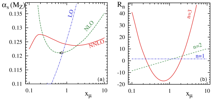
Figure 4: (a) $\alpha_{\rm s}(M_{\rm Z^{0}})$ determined from the scaled hadronic width of the $\rm Z^{0}$, $R_{\rm Z}=20.768$, in leading, next-to-leading and in next-to-next-to leading order QCD, as a function of the renormalization scale factor $x_{\mu}=\mu/M_{\rm Z^{0}}$. NLO solutions according to the PMS ($\bullet$), the EC ($\circ$) and the BLM ($\diamond$) scale optimization methods are marked. (b) Scale dependence of the QCD coefficients $R_{n}$ of $R_{\rm Z}$.

A practical example of the scale dependence of $\alpha_{\rm s}$, determined from the measured value of the scaled hadronic decay width of the $\rm Z^{0}$ boson [15],

$$R_{\rm Z}=\frac{\Gamma(\rm Z^{0}\rightarrow{\rm hadrons})}{\Gamma(\rm Z^{0}\rightarrow{\rm leptons})}=20.768\pm 0.0024\ ,$$ (14)

is shown in figure 4. QCD predictions of $R_{\rm Z}$ are available in complete NNLO [16]. Including further corrections like quark mass and non-factorizable electroweak and QCD effects, these predictions can be parametrised [17] to

$$R_{\rm Z}=19.934\left[1+1.045\frac{\alpha_{\rm s}(\mu)}{\pi}+0.94\left[\frac{\alpha_{\rm s}(\mu)}{\pi}\right]^{2}-15\left[\frac{\alpha_{\rm s}(\mu)}{\pi}\right]^{3}\right]\ ,$$ (15)

for $\mu\equiv M_{\rm Z^{0}}$; see section 4.3 for more details. In order to demonstrate the scale dependence of $\alpha_{\rm s}$, $\alpha_{\rm s}(\mu)$ is determined from equations 14 and 15 in LO, in NLO and in NNLO, as a function of the scaled renormalization scale, $x_{\mu}=\mu/M_{\rm Z^{0}}$, using the appropriate, scale dependent QCD coefficients $R_{n}$ according to equation 13. $\alpha_{\rm s}(M_{\rm Z^{0}})$ is then calculated from $\alpha_{\rm s}(\mu)$ using equation 2.4 in 1-loop expansion for the LO, in 2-loop for the NLO and in 3-loop for the NNLO case.

The resulting scale dependence of $\alpha_{\rm s}(M_{\rm Z^{0}})$ is displayed in figure 4(a); the scale dependence of the QCD coefficients $R_{1}$, $R_{2}$ and $R_{3}$ is given in figure 4(b). The scale dependence of $\alpha_{\rm s}$ is visibly reduced if higher orders are included: limiting renormalization scales to factors from 1/5 to 5 of the “physical” scale $Q\equiv M_{\rm Z^{0}}$, results in changes of $\alpha_{\rm s}(M_{\rm Z^{0}})$ of about 40% in LO, 8% in NLO and 2.5% in NNLO. Beyond these limits, however, the scale dependence even in NNLO QCD diverges, such that it seems not to be meaningful to consider yet larger ranges of scale factors $x_{\mu}$ - although there is no rule, from first principles, which limits scale variations to a definite range.

There are several proposals to optimize or to fix the renormalization scale in finite order perturbation theory. An intuitive approach is to apply the general scale insensitivity requirement, equation 1, which is strictly valid in infinite order, to calculations in any finite (beyond leading) order. This is Stevenson’s principle of minimal sensitivity (PMS)[18], where, for each observable $\cal{R}$, the optimal scale is defined by d$\cal{R}/\rm{d}\mu^{2}=0$. The PMS solution for $R_{\rm Z}$ in NLO is marked in figure 4(a) [filled circle].

In the “effective charge” method (EC) of Grunberg [19], all higher (i.e. beyond leading) order coefficients $R_{n}$ vanish. The EC solution in NLO is also marked in figure 4(a) [open circle].

Brodsky, Lepage and Mackenzie (BLM) [20] propose to choose $\mu$ such that the NLO coefficient $R_{2}$ is independent of $N_{f}$, the number of active quark flavours. The BLM solution is marked in figure 4(a) [open rhombus].

PMS, EC and BLM all provide unambiguous solutions in NLO; in the case of $R_{\rm Z}$, they are very close to each other but the NNLO prediction does not exactly match these results: the value of $\alpha_{\rm s}$ from “optimized” NLO can only be reached in NNLO at very small values of $x_{\mu}$.

While in NLO QCD it is sufficient to vary the renormalization scale in order to assess the full spectrum of variation offered by the renormalization procedure, in NNLO $both$ scale- and scheme-dependences must be taken into account. PMS, EC and BLM can then be generalized to NNLO and beyond, however do not lead to unambiguous results anymore. The whole issue of theoretical scale optimizations was and still is vividly discussed in the literature, see e.g. [21].

Another approach is motivated by an experimental point of view: ideally, the optimal choice of $\mu$ in a given order of perturbation theory should reproduce or, at least, closely approach the unknown all-order result. Measurements of observables should inherently include all orders of perturbation theory; therefore it may be possible to extract the optimal choice of $\mu$ in a given, finite order calculation from fits to the experimental data. Indeed, experimental scale optimization is possible in cases where $\alpha_{\rm s}$ is determined from differential $distributions$ of observables, and often leads to a remarkable consistency between results obtained from different observables [22, 23, 24, 25].

So far, none of the methods described above was generally accepted as $the$ preferred method to optimize or fix renormalistaion scales in finite order calculations. Instead, in experimental determinations of $\alpha_{\rm s}$, systematic uncertainties due to unknown higher order contributions are usually defined by allowing the renormalization scale $\mu$ to vary in “reasonable” ranges.

Unfortunately, there is no common agreement on what should be a reasonable range, and the significance and interpretation of such procedures is unclear. Furthermore, as indicated above, scale changes alone are not sufficient to investigate higher order uncertainties in NNLO predictions, where renormalization scheme dependences should also be accounted for.

2.8 Lattice QCD

At large distances or low momentum transfers, $\alpha_{\rm s}$ becomes large and application of perturbation theory becomes inappropriate. In this regime, nonperturbative methods must be used to describe processes of the Strong Interaction. Lattice QCD is one of the most developed nonperturbative methods which is used to calculate, for instance, hadron masses, hadron mass splittings and QCD matrix elements. In Lattice QCD, field operators are applied on a discrete, 4-dimensional Euclidean space-time of hypercubes with side length $a$.

Energy levels of heavy quarkonia systems ($Q\overline{Q}$) calculated using lattice QCD depend on the heavy quark mass $M_{Q}$ and on $\alpha_{\rm s}$. Comparison with measurements of quarkonia mass splittings then allows to determine $\alpha_{\rm s}$, which at this point is not given in the $\overline{\mbox{MS}}$ renormalization scheme but is based on other suitable definitions of $\alpha_{\rm s}$ on the lattice. Conversion from the lattice to the $\overline{\mbox{MS}}$ coupling at high energies can be done using an expansion in second or in third order perturbation theory. A review of methods to determine $\alpha_{\rm s}$ from lattice investigations is given in [26]

So far, calculations exist which either neglect light quark loop contributions ($N_{f}$=0; “quenched approximation”) or which include two light quark flavours ($N_{f}$=2); the latter allow extrapolation to $N_{f}$=3. Uncertainties in this extrapolation, the limited order to which the conversion to the $\overline{\mbox{MS}}$ scheme is known, limited Monte-Carlo statistics and corrections for light quark masses lead to theoretical uncertainties of final ($\overline{\mbox{MS}}$) values of $\alpha_{\rm s}(M_{\rm Z^{0}})$.

3 Results from deep inelasting scattering processes

Measurements of the violation of Bjorken scaling in deep inelastic lepton-nucleon scattering belong to the earliest methods to determine $\alpha_{\rm s}$. The first significant determinations of $\alpha_{\rm s}$, i.e. those based at least on next-to-leading order (NLO) perturbative QCD prediction, started to emerge in 1979 [27].

Today, a large number of results is available, from data in the energy ($Q^{2}$) range of a few to several thousand GeV², using electron-, muon- and neutrino-beams on various fixed target materials (H, D, C, Fe and CaCO₃), as well as electron-proton or positron-proton colliding beams at HERA. In addition to scaling violations of structure functions, $\alpha_{\rm s}$ is also determined from moments of structure functions, from QCD sum rules and — as in ${\rm e^{+}\rm e^{-}}$ annihilation — from hadronic jet production and event shapes.

3.1 Scaling violations and moments of structure functions

Cross sections of physical processes in lepton-nucleon scattering and in hadron-hadron collisions depend on the quark- and gluon-densities in the nucleon. Assuming factorization between short-distance, hard scattering processes which can be calculated using QCD perturbation theory, and low-energy or long-range processes which are not accessible by perturbative methods, such cross sections are parametrized by a set of structure functions $F_{i}$ ($i$= 1,2,3). The transition between the long- and the short-range regimes is defined by an arbitrary factorization scale $\mu_{f}$, which — in general — is independent from the renormalization scale $\mu$, but has similar features as the latter: the higher order coefficients of the perturbative QCD series for physical cross sections depend on $\mu_{f}$ in such a way that the cross section to all orders must be independent of $\mu_{f}$, i.e. $\partial\sigma/\partial\mu_{f}=0$. To simplify application of theory to experimental measurements, the assumption $\mu_{f}=\mu$ is usually made, with $\mu\equiv Q$ as the standard choice of scales.

In the naive quark-parton model, i.e. neglecting gluons and QCD, the differential cross sections for electromagnetic charged lepton (electron or muon) or weak neutrino-proton scattering off an unpolarized proton target are written

$$\frac{{\rm d}^{2}\sigma^{em}}{{\rm d}x{\rm d}y} \sim \frac{1+(1-y)^{2}}{2}2xF_{1}+(1-y)(F^{em}_{2}-2xF^{em}_{1})-\frac{M}{2E}xyF^{em}_{2}\ ;$$

$$\frac{{\rm d}^{2}\sigma^{\nu}}{{\rm d}x{\rm d}y} \sim \left(1-y-\frac{M}{2E}xy\right)F^{\nu}_{2}+y^{2}xF^{\nu}_{1}+y\left(1-\frac{1}{2}y\right)xF^{\nu}_{3}\ ,$$ (16)

where $x=\frac{Q^{2}}{2M(E-E^{\prime})}$ is the momentum fraction of the nucleon carried by the struck parton, $y=1-E^{\prime}/E$, $Q^{2}$ is the negative quadratic momentum transfer in the scattering process, and $M$, $E$ and $E^{\prime}$ are the mass of the proton and the lepton energies before and after the scattering, respectively, in the rest frame of the proton. In the quark-parton model, these structure functions consist of combinations of the quark- and antiquark densities $q(x)$ and $\overline{q}(x)$ for both valence- (u,d) and sea-quarks (s,c).

In QCD, the gluon content of the proton as well as higher order diagrams describing photon/gluon scattering, $\gamma g\rightarrow q\overline{q}$, and gluon radiation off quarks must be taken into account. Quark- and gluon-densities, the structure functions $F_{i}$ and physical cross sections become energy ($Q^{2}$) dependent. QCD thus predicts, departing from the naive quark-parton model, scaling violations in physical cross sections, which are associated with the radiation of gluons. While perturbative QCD cannot predict the functional form of parton densities and structure functions, their energy evolution is described by the so-called DGLAP equations [28, 29].

Structure functions contain, apart from terms whose energy dependence is given by perturbative QCD, which so far is known up to complete NLO [30], so-called “higher twist” contributions (HT). The leading higher twist terms are proportional to $1/Q^{2}$; they are numerically important at low $Q^{2}<\cal{O}$(few GeV${}^{2})$ and at very large $x\simeq 1$.

Historically, precise results of $\alpha_{\rm s}$, from the logarithmic slopes of $F_{2}(x,Q^{2})$ and in NLO QCD, were obtained from a combined analysis [31] of SLAC and BCDMS data, in a $Q^{2}$ range from 0.5 to 260 GeV², giving $\alpha_{\rm s}(M_{\rm Z^{0}})=0.113\pm 0.005$. The error includes theoretical (scale) uncertainties of $\pm 0.004$ [32]. Higher twist terms as well as the gluon distribution were simultaneously determined in this analysis.

The CCFR colaboration obtained $\alpha_{\rm s}$ from $\nu$-nucleon scattering and a fit to the non-singlet structure function $F_{3}(x,Q^{2})$ [33], which is independent of the poorly known gluon distribution. In order to increase statistical precision, $F_{3}$ was substituted by $F_{2}$ at large $x$ where gluons do not contribute much, giving $\alpha_{\rm s}(M_{\rm Z^{0}})=0.111\pm 0.002{\rm(stat.)}\pm 0.003{\rm(sys.)}\pm 0.004{\rm(theo.)}$.

These two results were, for several years, the most significant from deep inelastic lepton-nucleon scattering. Because they were numerically smaller than typical values obtained from ${\rm e^{+}\rm e^{-}}$ annihilation, $\alpha_{\rm s}(M_{\rm Z^{0}})\sim 0.120$ (see Section 4), speculations about possible reasons for such differences arose. These speculations came to a halt, at least partly, when the CCFR collaboration corrected their previous result — due to a new energy calibration of the detector — to $\alpha_{\rm s}(M_{\rm Z^{0}})=0.119\pm 0.005$ [34]. Further results from $F_{2}$, in a study [35] of the HERA data at small $x$ and $Q^{2}<100~{}{\rm GeV}^{2}$, based on NLO QCD including summations of all leading and subleading logarithms of $Q^{2}$ and $1/x$, lead to $\alpha_{\rm s}(M_{\rm Z^{0}})=0.120\pm 0.005\pm 0.009$, where the first error is experimental and the second theoretical. Finally, a reanalysis of the SLAC, BCDMS and NMC data on $F_{2}$, taking proper account of point-to-point correlations, resulted in an increase of $\alpha_{\rm s}(M_{\rm Z^{0}})$ from 0.113 to 0.118 [36]. A continuation of this analysis, including recent HERA data and careful studies of the effects of higher twist terms, was reported to result in $\alpha_{\rm s}(M_{\rm Z^{0}})=0.116\pm 0.003$ [37].

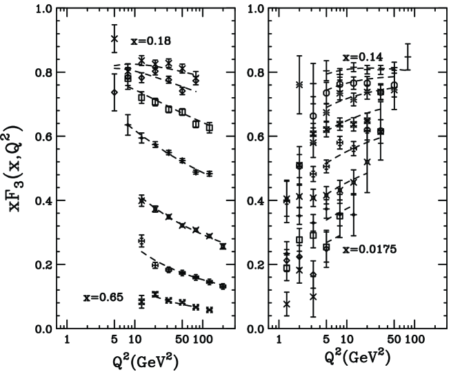
Figure 5: Comparison of CCFR data [34] with NNLO QCD fits [38].

Significant progress in this field was achieved with the availability of NNLO QCD predictions for the non-singlet structure function $F_{3}$ as well as for moments of $F_{2}$. A new analysis [38] of the CCFR data, now in NNLO QCD and from $xF_{3}$ alone, resulted in

$$\alpha_{\rm s}(M_{\rm Z^{0}})=0.118\pm 0.002{\rm(stat.)}\pm 0.005{\rm(sys.)}\pm 0.003{\rm(theo.)}\ ;$$

see figure 5. This value is taken as the currently most significant result from structure functions in neutrino-nucleon deep inelastic scattering, and is included in the final summary, see Table 6. Another recent study was based on Bernstein polynomials and moments of ${\rm F}_{2}$ from electron- and muon-scattering data, including fixed target as well as HERA colliding beam data in the $Q^{2}$ range of 2.5 to 230 GeV². The result [39] was

$$\alpha_{\rm s}(M_{\rm Z^{0}})=0.1172\pm 0.0017\pm 0.0017\ ,$$

where the first error is experimental and the second theoretical. The theoretical error includes higher twist effects and an estimate of the NNNLO corrections. This result is taken as the final value from $F_{2}$ in DIS and is added to the summary in section 7.

From scaling violations of polarized structure functions, based on data from SLAC and SMC, $\alpha_{\rm s}$ was determined [40] in NLO QCD, resulting in

$$\alpha_{\rm s}(M_{\rm Z^{0}})=0.120^{+0.004}_{-0.005}{\rm(exp.)}^{+0.009}_{-0.006}{\rm(theo.)}\ ,$$

which is also added to the final summary.

3.2 Sum Rules

Perturbative corrections to two inclusive measurements, namely the Gross-Llewellyn Smith (GLS) sum rule [41] for deep inelastic neutrino scattering and the Bjorken sum rule [42] for polarized structure functions, have been determined to complete NNLO QCD [43, 44]. The GLS sum rule,

$${\rm GLS}=\int^{1}_{0}F_{3}(x,Q^{2}){\rm d}x\ \equiv\ 3(1-\frac{\alpha_{\rm s}}{\pi}+\dots),$$ (17)

when fitted to data of the CCFR collaboration [45] at $Q^{2}=3\ {\rm GeV}^{2}$, resulted in [43] $\alpha_{\rm s}(1.73\ {\rm GeV})=0.32\pm 0.05$. A recent update of the data and analysis from CCFR [46], in the $Q^{2}$ range from 1 to 15.5 GeV², gave

$$\alpha_{\rm s}(1.73\ {\rm GeV})=0.28\pm 0.035{\rm(stat.)}\pm 0.050{\rm(sys.)}^{+0.035}_{-0.030}{\rm(theo.)}\ .$$

The systematic uncertainty is dominated by the extrapolation of the GLS integral to the regions $x<0.01$ where no measurements exist, and to $x>0.5$ which is substituted by $F_{2}$ from SLAC data, see figure 6. The theoretical error is dominated by uncertainties in the higher twist corrections.

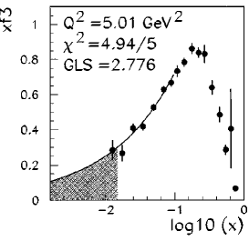
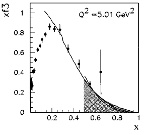
Figure 6: $xF_{3}$ as a function of $x$ at $Q^{2}=5$ GeV², with a power law fit to the region $x<0.1$ (left figure; logarithmic $x$-scale) and the shape of the SLAC $F_{2}$ data for $x>0.5$ (right figure; linear $x$-scale) which are used to calculate the GLS integral in the shaded regions (figures from [46]).

The Bjorken polarized sum rule determines that

$$\int_{0}^{1}\left[g_{1}^{p}(x)-g_{1}^{n}(x)\right]{\rm d}x=\frac{1}{3}\left|\frac{g_{A}}{g_{V}}\right|\left(1-\frac{\alpha_{\rm s}}{\pi}+\dots\right),$$ (18)

where the polarized structure functions $g_{1}(x)$ for protons (superscript $p$) and neutrons ($n$) are derived from the difference of cross sections for parallel and antiparallel polarized targets and ($\mu$ or e) beams; $g_{A}$ and $g_{V}$ are the constants of the neutron weak decay, $g_{A}/g_{V}=-1.26$. A study [47] of the CERN SMC [48] and the SLAC E142 [49] data obtained

$$\alpha_{\rm s}(1.58\ {\rm GeV})=0.375^{+0.062}_{-0.081}.$$

No explicit corrections for nonperturbative higher twist where applied to derive this result, however an estimate of the size of the ${\cal O}(\alpha_{\rm s}^{4})$ terms [50] was taken into account.

3.3 Jet Production and Event Shapes

Observables parametrizing hadronic event shapes and jet production rates are the classical inputs for $\alpha_{\rm s}$ studies in ${\rm e^{+}\rm e^{-}}$ annihilation. In recent years, these observables were also studied in high energetic electron- and positron-proton collisons at HERA, leading to significant determinations of $\alpha_{\rm s}$.

In detail, inclusive as well as differential jet production rates were studied in the energy range of $Q^{2}\sim 10$ up to 10000 GeV² [51], using variants of jet algorithms from ${\rm e^{+}\rm e^{-}}$ annihilation which are decribed, in more detail, in section 4. In leading order $\alpha_{\rm s}$, 2 + 1 jet events in deep inelastic $ep$ scattering arise from photon-gluon fusion and from QCD compton processes. The term ‘2 + 1 jet’ denotes events where two resolved jets can be identified, in addition to the beam jet from the remnants of the incoming proton. Previous NLO QCD predictions [52] which were shown to be imprecise are now replaced by more recent calculations [53].

The results of $\alpha_{\rm s}$ from jet production at HERA [51] can be summarized to

$$\alpha_{\rm s}(M_{\rm Z^{0}})=0.118\pm 0.002{\rm(stat.)}\pm 0.008{\rm(sys.)}\pm 0.007{\rm(theo.)}\ .$$

The systematic error contains uncertainties from using different jet algorithms and hadronization models, and the theoretical error is dominated by uncertainties from structure functions and from scale variations.

So far, studies of $\alpha_{\rm s}$ from hadronic event shape distributions at HERA [54] are based on fits to the energy ($Q^{2}$) evolution of mean values of shape distributions, using NLO QCD predictions together with parametrizations of power corrections $1/Q^{p}$ [55]. These methods do not yet lead to consistent results of $\alpha_{\rm s}$ from different shape observables [54] — at least not to the degree of precision which is obtained from “classical” studies of $\alpha_{\rm s}$ from event shape distributions, as e.g. in ${\rm e^{+}\rm e^{-}}$ annihilation; see Section 4.1 for further discussion. Awaiting further progress in theoretical understanding of power corrections to event shapes, the $\alpha_{\rm s}$ results of these studies will not yet be included in the final summary of $\alpha_{\rm s}$.

4 Results from ${\rm e^{+}\rm e^{-}}$ annihilation

In ${\rm e^{+}\rm e^{-}}$ annihilation reactions, $\alpha_{\rm s}$ is classically determined from hadronic event shapes, jet production rates and energy correlations for which complete NLO QCD calculations are available [56, 57, 58]. The first data analysis of this type, from jet rates observed at the PETRA ${\rm e^{+}\rm e^{-}}$ collider, emerged in 1982 [59]. Reviews of early results on $\alpha_{\rm s}$ from ${\rm e^{+}\rm e^{-}}$ annihilations can be found e.g. in references [60, 61].

More recently, this field was extensively covered by the experiments at the LEP and SLC colliders, see e.g. [62, 63, 64, 65, 66] for reviews of the first few years of LEP operation. Using data from LEP and from earlier ${\rm e^{+}\rm e^{-}}$ colliders at lower c.m. energies, $\alpha_{\rm s}$ can be determined from scaling violations of fragmentation functions. Most importantly, precise determinations of $\alpha_{\rm s}$ are now obtained from the hadronic partial width of $\rm Z^{0}$ decays, from overall fits to precision electroweak data and from hadronic branching fractions of $\tau$ lepton decays, which are calculated in complete NNLO QCD.

4.1 Event shapes, jet rates and energy correlations

4.1.1 Observables in (resummed) NLO QCD

Hadronic event shape variables, jet rates and energy correlations are tools to study both the amount of gluon radiation and details of the hadronization process. The definitions of observables which are applied to hadronic final states of ${\rm e^{+}\rm e^{-}}$ annihilations, like Thrust, Thrust Major and Minor, Oblateness, jet masses, the jet broadening measures, energy correlations and jet production rates, are summarized elsewhere; see e.g. [57, 67, 68, 69]. Only two of these, the Thrust observable and the JADE jet algorithm shall be described here in some more detail:

The Thrust $T$ [70] is the normalized sum of the momentum components $\vec{p}_{i}\vec{n}$ of all particles $i$ of a given event along a specific axis $\vec{n}$; the axis is chosen such that $T$ is maximized:

$$T={\rm max}\left(\frac{\sum_{i}|\vec{p}_{i}\vec{n}|}{\sum_{i}|\vec{p}_{i}|}\right)\ .$$

Thrust assumes values of $T=1$ for perfectly aligned momentum vectors, i.e. for an ideal event ${\rm e^{+}\rm e^{-}}\rightarrow q\overline{q}$ with two narrow back-to-back jets, down to $T=0.5$ for a completely spherical distribution of momentum vectors in the limit of events with many gluons radiated off the initial $q\overline{q}$ pair.

Within the JADE jet algorithm [71], the scaled pair mass of two resolvable jets $i$ and $j$, $y_{ij}=M_{ij}^{2}/E_{vis}^{2}$, is required to exceed a threshold value $y_{cut}$, where $E_{vis}$ is the sum of the measured energies of all particles of an event. In a recursive process, the pair of particles or clusters of particles $n$ and $m$ with the smallest value of $y_{nm}$ is replaced by (or “recombined” into) a single jet or cluster $k$ with four-momentum $p_{k}=p_{n}+p_{m}$, as long as $y_{nm}<y_{\rm cut}$. The procedure is repeated until all pair masses $y_{ij}$ are larger than the jet resolution parameter $y_{\rm cut}$, and the remaining clusters of particles are called jets.

Several jet recombination schemes and definitions of $M_{ij}$ exist [57, 67, 72]; the original JADE scheme with $M_{ij}^{2}=2\cdot E_{i}\cdot E_{j}\cdot(1-\cos{\theta_{ij}})$, where $E_{i}$ and $E_{j}$ are the energies of the particles and $\theta_{ij}$ is the angle between them, and the “Durham” scheme [73, 67] with $M_{ij}^{2}=2\cdot{\rm min}(E_{i}^{2},E_{j}^{2})\cdot(1-\cos{\theta_{ij}})$, were most widely used at LEP, due to their superior features like small sensitivity to hadronization and particle mass effects [67].

QCD predictions for hadronic event shapes, of jet production rates and of energy correlations are available in complete NLO [56, 57, 58]. Differential distributions of such observables $y$ are parametrized as

$$\frac{1}{\sigma_{0}}\frac{{\rm d}\sigma}{{\rm d}y}=R_{1}(y)\alpha_{\rm s}(\mu^{2})+R_{2}(y,Q^{2}/\mu^{2})\alpha_{\rm s}^{2}(\mu^{2})\ ,$$ (19)

where $\sigma_{0}$ is the total hadronic cross section in leading order. In addition, for some of the observables, resummation of the leading and next-to-leading logarithms (NLLA) is available [14] which can be matched with the NLO expressions (resummed NLO); see section 2.6.

In a typical study, measured distributions are corrected for effects of limited detector acceptance and resolution. Fits of QCD predictions to the data are performed after applying hadronization corrections, as predicted from hadronization models, to the data or to the theoretical predictions. Systematic uncertainties due to these corrections, from renormalization scale variations and from different matching procedures, are studied and included in the overall error of the fitted value of $\alpha_{\rm s}$. No common agreement exists, however, about the range of variations used to estimate these uncertainties.

Early determinations of $\alpha_{\rm s}$ from event shapes, jet rates and energy correlations obtained from experiments at the PETRA and PEP colliders were summarized to $\alpha_{\rm s}=0.14\pm 0.02$ at $Q^{2}=E_{cm}^{2}\sim(34\ {\rm GeV})^{2}$ [60, 61], in NLO QCD. The results which led to this average did not include estimates of theoretical uncertainties; however the error was determined from the scatter of the single results which were based on different observables, and thus gave a first estimate of theoretical uncertainties.

4.1.2 Results in resummed NLO

A reanalysis of PETRA data, using refined analysis techniques, resummed NLO QCD calculations, modern model calculations and including new observables, quite similar to recent analyses at LEP, resulted in [74]

$$\alpha_{\rm s}\left(22\ {\rm GeV}\right) = 0.161\pm 0.009\pm^{+0.014}_{-0.006}\ ,$$

$$\alpha_{\rm s}\left(35\ {\rm GeV}\right) = 0.145\pm 0.002^{+0.012}_{-0.007}\ ,\ {\rm and}$$

$$\alpha_{\rm s}\left(44\ {\rm GeV}\right) = 0.139\pm 0.004^{+0.010}_{-0.007},$$

where the first errors are statistical and experimental systematic, added in quadrature, and the second are theoretical uncertainties. These values are taken as the final results in the PETRA energy range and are included in the summary table 6. Similar analyses from experiments at the TRISTAN collider, around c.m. energies of 58 GeV, gave [75]

$$\alpha_{\rm s}\left(58\ {\rm GeV}\right)=0.132\pm 0.008\ ,$$

which is also included in the summary.

Figure 7: Differential Thrust distributions measured at various c.m. energies at LEP (symbols), together with resummed NLO QCD fits (lines; figure adapted from [76]).

At the LEP collider, all four experiments (ALEPH, DELPHI, L3 and OPAL) have contributed a multitude of studies based on the high statistics data samples around the $\rm Z^{0}$ resonance (LEP-I; $E_{cm}\sim 91.2$ GeV) and at the higher energies of the LEP-II running phase ($E_{cm}\sim 133,\ 161,\ 172,\ 183$ and 189 GeV). The SLD experiment at the SLAC Linear Collider (SLC) contributed similar studies at $E_{cm}\sim M_{\rm Z^{0}}$. As an example of the precise description of data by the CQD fits, the Thrust distributions as measured by ALEPH at LEP-I and LEP-II energies are shown in figure 7, together with the corresponding fits of the resummed NLO QCD calculations.

The most current results from LEP and SLC, based on resummed NLO QCD calculations, are taken from [76, 77, 78, 79, 80] and are combined to obtain one single value of $\alpha_{\rm s}$ at each c.m. energy. This is done by calculating weighted averages of the results quoted by each experiment, with the inverse quadratic total error taken as the weight. The experimental uncertainties are combined assuming that no correlation exists between the experiments. Theoretical uncertainties are assumed to be common to all experiments, however different methods and definitions were used to estimate these in each case. Therefore, a linear average of the theoretical uncertainties quoted by the experiments is used to define the theoretical error of the combined results. This gives

$$\alpha_{\rm s}\left(91.2\ {\rm GeV}\right) = 0.121\pm 0.001\pm 0.006\ ,$$

$$\alpha_{\rm s}\left(133\ {\rm GeV}\right) = 0.113\pm 0.003\pm 0.006\ ,$$

$$\alpha_{\rm s}\left(161\ {\rm GeV}\right) = 0.109\pm 0.004\pm 0.005\ ,$$

$$\alpha_{\rm s}\left(172\ {\rm GeV}\right) = 0.104\pm 0.004\pm 0.005\ ,$$

$$\alpha_{\rm s}\left(183\ {\rm GeV}\right) = 0.109\pm 0.002\pm 0.004\ ,$$

$$\alpha_{\rm s}\left(189\ {\rm GeV}\right) = 0.110\pm 0.001\pm 0.004\ ,$$

where the first errors are experimental and the second theoretical. These results are included in the final summary table 6. Note, however, that some of the averages at LEP-II energies contain results which are still preliminary, see [76, 77, 78, 79].

The energy dependence of $\alpha_{\rm s}$ from studies of event shape observables is clearly seen in the results presented above. This is also demonstrated in a dedicated analysis of the L3 Collaboration [81] which includes a study of radiative events recorded at LEP-I. Such events are effectively produced at reduced hadronic centre of mass energies; they can therefore be used to determine $\alpha_{\rm s}$ at energy scales below the nominal collider energy. The statistical precision at these reduced energies is, however, limited.

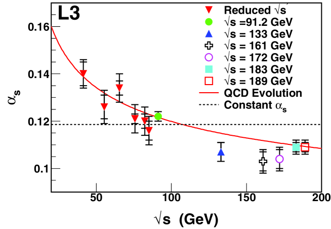
Figure 8: Running of $\alpha_{\rm s}$ from hadronic event shapes at LEP, measured by L3. The results at energies below 91 GeV are from radiative events at $2E_{beam}\approx M_{\rm Z^{0}}$ (figure from reference [81]).

The results of the L3 study are shown in figure 8, demonstrating the agreement of the data with the QCD expectation of a running coupling. Note that, in order to judge the significance for the running, only the innermost, experimental errors must be taken into account, since theoretical uncertainties are highly correlated between the different data points. The running of $\alpha_{\rm s}$ was also demonstrated in a recent study of jet production rates at PETRA and at LEP energies, using the same consistent analysis method and data from two experiments comprising similar detector techniques, JADE and OPAL [82].

Before the advent of resummed QCD calculations for event shape observables, determinations of $\alpha_{\rm s}$ were done in pure NLO, see e.g. [23, 24]. Studies of theoretical uncertainties typically included scale variations from $x_{\mu}=1$ down to the best fit values of $x_{\mu}$, from two-parameter fits, or the optimized scales given by the methods discussed in Section 2.7 . These ranges were quite large, down to $x_{\mu}\sim 0.01$, which lead to rather large scale uncertainties in case of some of the observables. Resummed NLO results, however, had smaller dependencies on scale variations, as theoretically expected, which is why they developed as a standard in $\alpha_{\rm s}$ determinations from event shape studies.

4.1.3 Pure NLO results

Fits of pure NLO QCD to experimental event shape and jet rate distributions are known to provide a consistent description of the data if - in addition to $\alpha_{\rm s}$ - also the renormalization scale is treated as a free parameter of the fit [22]. While the fitted scale factor $x_{\mu}$ assumes different values for different observables, indicating that the amount of unknown, higher order contributions is different in each case, the resulting value of $\alpha_{\rm s}$ appears to be “universal” and in much better agreement than applying a single and fixed choice of scale [23, 24].

These findings are corroborated in a recent re-analysis of DELPHI data at LEP-I [83], which also demonstrates that experimentally optimized NLO calculations can provide a more consistent description of the data than resummed NLO at fixed scale $x_{\mu}=1$. Defining a scale range, for each observable, of a factor of 2 around the experimental fit value of $x_{\mu}^{2}$, results in $\alpha_{\rm s}(M_{\rm Z^{0}})=0.1174\pm 0.0026$, which includes both experimental and theoretical uncertainties. This method of optimizing renormalization scales and defining the size of the remaining theoretical uncertainties seems logical from an experimental point of view, see the discussion in Section 2.7, but carries intrinsic theoretical problems:

Firstly, the resulting scale factors are rather small, down to $\cal{O}$(0.01) or smaller, such that large logarithms appear in the NLO coefficients, see equation 13. Secondly, there is no common agreement about the significance of $one$ overall scale for each distribution because theoretical scale optimizations predict $x_{\mu}$ to depend on the value of the observable itself. The issue of experimental scale optimization therefore requires further investigation and discussion.

4.1.4 Power corrections

In the past few years, analytical approaches were pursued to approximate nonperturbative hadronization effects by means of perturbative methods, introducing a universal, non-perturbative parameter

$$\alpha_{0}(\mu_{I})=\frac{1}{\mu_{I}}\int^{\mu_{I}}_{0}{\rm d}k\ \alpha_{\rm s}(k)$$

to parametrize the unknown behaviour of $\alpha_{\rm s}(Q)$ below a certain infrared matching scale $\mu_{I}$ [84]. Divergent soft gluon contributions to the perturbative predictions of event shapes are removed and, as a consequence of these techniques, lead to corrections which are proportional to powers of $1/Q$. Power corrections are regarded as an alternative approach to describe hadronization effects on event shape distributions, instead of using phenomenological hadronization models as in the studies discussed in the previous sections.

The energy dependence of event shape distributions and of their integrated mean values, in the c.m. energy range from 14 to 183 GeV, were analysed and compared with perturbative QCD calculations plus added power corrections [74, 85, 76, 77]. Two-parameter fits of $\alpha_{0}$ and $\alpha_{\rm s}(M_{\rm Z^{0}})$ to the data provide a consistent description of the shapes and the energy evolution of the data; however the scatter between results from different shape observables is larger than the typical uncertainties would suggest. The non-perturbative parameter $\alpha_{0}$ turns out to be universal for all studied observables within about 20%, and values of $\alpha_{\rm s}(M_{\rm Z^{0}})$ seem to be close to but systematically smaller than those from fits using conventional methods of hadronization corrections [85].

Power corrections, as an analytical ansatz to compute nonperturbative QCD corrections to event shape observables, offer a rather promising alternative to the use of phenomenological hadronization models in determinations of $\alpha_{\rm s}$; however more experience, confidence and further developments are necessary before actual fit results of $\alpha_{\rm s}$ can supersede the results from “classical” event shape analyses described above.

4.2 $\alpha_{\rm s}$ from scaling violations of fragmentation functions

The total cross section of ${\rm e^{+}\rm e^{-}}$ annihilations into charged hadrons $h$, ${\rm e^{+}\rm e^{-}}\rightarrow h+X$, can be factorized into a perturbative and a nonperturbative regime, describing processes of hard gluon radiation and of hadronization, respectively. The perturbative part can be calculated in terms of so-called coefficient functions, while the non-perturbative part is parametrized by phenomenological fragmentations functions. The separation of these two regimes is performed at an energy scale $\mu_{f}$, the factorisation scale, which — as in DIS — enters as a second, arbitrary energy scale, in addition to the renormalization scale $\mu$. According to the factorization theorem, the cross section can then be written [86]:

$$\frac{{\rm d}\sigma}{{\rm d}x}({\rm e^{+}\rm e^{-}}\rightarrow h+X)=\sum_{i}\int^{1}_{x}\frac{{\rm d}z}{z}\ C_{i}\left(z,\alpha_{\rm s}(\mu^{2}),\mu^{2}/Q^{2}\right)\ D_{i}\left(x/z,\mu_{f}^{2}\right)\ ,$$ (20)

where $C_{i}$ are the coefficient functions for creating a parton with flavour $i$ and momentum fraction $z=p_{parton}/p_{beam}$, $D_{i}$ represent the probability that parton $i$ fragments into a hadron $h$ with momentum fraction $x/z$, and $x=p_{hadron}/p_{beam}$.

In lowest order, the coefficient functions $C_{i}$ are given by the electroweak couplings for quarks; they vanish for gluons. Higher order QCD corrections apply to the quark coefficient functions and lead to finite functions for gluons, too. These corrections are known up to complete NLO [87], however only the LO corrections were available and used in currently existing analyses.

The fragmentation functions $D_{i}$ are not given by perturbation theory; however — as in the case of parton densities and structure functions (c.f. Section 3.1) — their energy dependence is described by QCD via complicated integro-differential equations and the DGLAP evolution functions [28, 29].

The ALEPH [88] and the DELPHI [89] collaborations at LEP have both published detailed analyses of the charged hadron fragmentation functions, using data samples from the PETRA, PEP and LEP colliders spanning c.m. energy ranges from 14 to 91.2 GeV. At LEP, ALEPH and DELPHI extracted differential $x$ distributions separately for initial b-, c- and uds-quark events, and obtained the corresponding gluon-jet distribution from tagged gluon jet event samples. Assuming a certain parametrization of the “bare” fragmentation functions at a “starting energy scale” $Q_{0}$, $\alpha_{\rm s}(M_{\rm Z^{0}})$, the free parameters of the starting fragmentation functions for gluons and the different quark flavours, as well as a parameter allowing for additional, nonperturbative power law corrections, are determined in fits to all experimental $x$-distributions.

Combining both the ALEPH and the DELPHI results, which are based on comparable data sets and analysis strategies, leads to

$$\alpha_{\rm s}(M_{\rm Z^{0}})=0.125^{+0.006}_{-0.007}\ {\rm(exp.)}\ \pm 0.009\ {\rm(theo.)}\,$$

where the theoretical uncertainty includes variations of both the factorization and the renormalization scales.

4.3 $\alpha_{\rm s}$ from total hadronic cross sections

Because of its inclusive nature, the total cross section of the process ${\rm e^{+}\rm e^{-}}\rightarrow$ hadrons was the first quantity for which QCD corrections up to complete NNLO were known [90, 91]. For c.m. energies in the ${\rm e^{+}\rm e^{-}}$ continuum, far below the $\rm Z^{0}$ pole and for $\mu\equiv E_{cm}$, the normalized cross section is given by

$$R_{\gamma}=\frac{\sigma({\rm e^{+}\rm e^{-}}\rightarrow{\rm hadrons})}{\sigma({\rm e^{+}\rm e^{-}}\rightarrow\mu^{+}\mu^{-})}=3\sum_{i}q_{i}^{2}\left(1+\frac{\alpha_{\rm s}}{\pi}+1.441\left(\frac{\alpha_{\rm s}}{\pi}\right)^{2}-12.8\left(\frac{\alpha_{\rm s}}{\pi}\right)^{3}\right)\ ,$$ (21)

where $q_{i}$ are the electrical charges of quark flavours $i$ which are produced, i.e. for which $2M_{q}\ll E_{cm}$.

Because of the above functional form of $R_{\gamma}(\alpha_{\rm s})$, $relative$ errors of $R_{\gamma}$ lead to $absolute$ errors in $\alpha_{\rm s}$ of about the same size, $\Delta R/R\sim\Delta\alpha_{\rm s}$, such that precise measurements of $R$ still lead to rather large errors in $\alpha_{\rm s}$. As another complication, electroweak corrections due to real $\rm Z^{0}$ exchange and due to $\gamma-\rm Z^{0}$ interference must be applied to the data in the c.m. energy range above 20 GeV. These corrections are negligible at $E_{cm}$ = 14 GeV, but at $E_{cm}$ =46 GeV they amount to about the same size as the QCD corrections [92].

A combination of the cross section measurements of all four PETRA experiments, in the c.m. energy range of 14 to 46.8 GeV, accounting for correlated experimental uncertainties, electroweak corrections and leading order initial state radiation effects, resulted in $\alpha_{\rm s}{\rm(34\ GeV)}=0.169\pm 0.025$ [92], in NLO QCD. Applying the full NNLO QCD prediction which was not yet available at that time results in $\alpha_{\rm s}{\rm(34\ GeV)}=0.175\pm 0.028$ or — equivalently — in $\alpha_{\rm s}(M_{\rm Z^{0}})=0.143\pm 0.018$. Two groups have analysed and combined ${\rm e^{+}\rm e^{-}}$ hadronic cross sections measured in the c.m. energy ranges from 7 to 57 GeV [93] and from 2.65 to 52 GeV [94]. They both used an initially erroneous value of the NNLO QCD coefficient of $R_{\gamma}$, +64.8 instead of -12.8; when corrected for this mistake, they result in $\alpha_{\rm s}(34\ {\rm GeV})=0.165\pm 0.022$ [93] and in $\alpha_{\rm s}(31.6\ {\rm GeV})=0.158\pm 0.019$ [94]. Combining the two gives $\alpha_{\rm s}(34\ {\rm GeV})=0.160\pm 0.019\ {\rm(exp.+sys.)}$ or $\alpha_{\rm s}(M_{\rm Z^{0}})=0.133\pm 0.013$.

A re-analysis [95] of PETRA and TRISTAN data, in the c.m. energy range of 20 to 65 GeV, took better account of higher order QED and electroweak corrections and used the mass of the $\rm Z^{0}$ measured from LEP experiments. In NLO QCD, this study resulted in $\alpha_{\rm s}(M_{\rm Z^{0}})=0.124\pm 0.021$, where the error includes experimental and systematical uncertainties, added in quadrature. Re-applying the NNLO QCD correction this gives

$$\alpha_{\rm s}{\rm(42.4\ GeV)}=0.175\pm 0.028\ \ {\rm or}\ \ \alpha_{\rm s}(M_{\rm Z^{0}})=0.126\pm 0.022\ ,$$

which is included in the final summary section 7. A more recent determination of $\alpha_{\rm s}$ from the total ${\rm e^{+}\rm e^{-}}$ hadronic cross section measured by CLEO at $E_{cm}=10.52$ GeV [96] resulted in

$$\alpha_{\rm s}{\rm(10.52\ GeV)}=0.130\ ^{+\ 0.021\ }_{-\ 0.029\ }$$

and is also added to the final summary.

On top and around the $\rm Z^{0}$ resonance, the LEP experiments have collected large statistics data samples which allow accurate determinations of $\alpha_{\rm s}$. At the $\rm Z^{0}$ pole, equation 21 must be modified according to the dominant electroweak couplings of the $\rm Z^{0}$ to the quarks, resulting in NNLO QCD predictions of the hadronic decay width of the $\rm Z^{0}$ [16]. Quark mass corrections in NLO [10] and partly to NNLO [11], non-factorizable electroweak and QCD corrections [97], top quark effects and other electroweak corrections apply in addition, rendering numerical expressions for $R_{\rm Z}=\Gamma(\rm Z^{0}\rightarrow{\rm hadrons})/\Gamma(\rm Z^{0}\rightarrow{\rm leptons})$ rather complicated; see e.g. ref. [98] for a comprehensive report about QCD corrections on $R_{\gamma}$ and $R_{\rm Z}$.

In this review, a recent parametrisation of the NNLO QCD prediction of $R_{\rm Z}$ [17], including all known corrections indicated above, is applied to determine $\alpha_{\rm s}$ from $R_{\rm Z}$. This parametrisation, as given in equation 15, is also used by the LEP collaborations in their combined studies of electroweak precision data [15]. The coefficients given in equation 15 are calculated for a Higgs mass $M_{H}$ of 300 GeV, a top quark mass $M_{t}$ of 174.1 GeV and for $M_{\rm Z^{0}}$ = 91.19 GeV. With the latest combined LEP result, $R_{\rm Z}=20.768\pm 0.024$ [15], this gives $\alpha_{\rm s}(M_{\rm Z^{0}})=0.124\pm 0.004\ {\rm(exp.)}$.

Table 2: Estimates of errors in the determination of $\alpha_{\rm s}(M_{\rm Z^{0}})$ from $R_{\rm Z}$, caused by different sources of uncertainties.

error source	$\Delta\alpha_{\rm s}(M_{\rm Z^{0}})$
$\Delta M_{\rm Z^{0}}=\pm 0.0021\ {\rm GeV}$	$\pm 0.00003$
$\Delta M_{t}=\pm 5\ {\rm GeV}$	$\pm 0.0002$
$M_{H}=100\ ...\ 1000\ {\rm GeV}$	$\pm 0.0017$
$\mu=\left(\frac{1}{4}\ ...\ 4\right)\ M_{\rm Z^{0}}$	${}^{+\ 0.0028}_{-\ 0.0004}$
renormalization schemes	$\pm 0.0002$
total	${}^{+\ 0.003}_{-\ 0.002}$

Errors in $\alpha_{\rm s}(M_{\rm Z^{0}})$ from different sources, namely from changes of $M_{\rm Z^{0}}$ and $M_{t}$ within their current uncertainties, from $M_{H}$ in the range of 100 GeV (the current experimental lower limit from LEP) to 1000 GeV, and from renormalization scale uncertainties, varying $\mu$ from 1/4 to 4$M_{\rm Z^{0}}$, are given in Table 2. The estimate of the $scheme$ dependence, which in NNLO must be considered in addition to the renormalization $scale$ dependence, was taken from reference [99]. Neglecting the tiny errors from $M_{\rm Z^{0}}$ and from $M_{t}$, the overall theoretical uncertainty on $\alpha_{\rm s}(M_{\rm Z^{0}})$ from $R_{\rm Z}$ is estimated to be $\pm 0.002$ from $M_{H}$ and $M_{t}$ and ${}^{+\ 0.003}_{-\ 0.001}$ from higher order QCD contributions. Therefore, the final result from $R_{\rm Z}$, to be added to the overall summary, is

$$\alpha_{\rm s}(M_{\rm Z^{0}})=0.124\pm 0.004{\rm(exp.)}\pm 0.002(M_{H},M_{t})^{+\ 0.003}_{-\ 0.001}{\rm(QCD)}\ .$$

Note that the precision of this result crucially depends on the assumption that the predictions of the electroweak Standard Model are strictly valid; small deviations from these predictions can produce large systematic shifts of $\alpha_{\rm s}(M_{\rm Z^{0}})$ from $R_{\rm Z}$. The LEP data, however, are in excellent overall agreement with the Standard Model predictions [15], such that the uncertainties quoted above seem realistic.

A combined fit to all data from LEP-I and LEP-II, including the measurement of the mass of the W boson, $M_{W}$, and all measured cross sections and asymmetries, instead of $R_{\rm Z}$ alone, results in $\alpha_{\rm s}(M_{\rm Z^{0}})=0.120\pm 0.003{\rm(exp.)}$; a fit to all data including those from $p\overline{p}$ collider and lepton-nucleon scattering experiments gives $\alpha_{\rm s}(M_{\rm Z^{0}})=0.118\pm 0.003{\rm(exp.)}$ [15]. These fits include simultaneous determinations of $M_{H}$ and $M_{t}$, such that only the QCD uncertainty must be added. Because of their complicated nature, however, these results are only mentioned for completeness, but are not taken to replace the above value of $\alpha_{\rm s}(M_{\rm Z^{0}})$ from $R_{\rm Z}$ for the final summary.

4.4 $\alpha_{\rm s}$ from $\tau$ decays

An important quantity to determine $\alpha_{\rm s}$ from measurements at small energy scales is the normalized hadronic branching fraction of $\tau$ lepton decays,

$$R_{\tau}=\frac{\Gamma(\tau\rightarrow{\rm hadrons}\ \nu_{\tau})}{\Gamma(\tau\rightarrow{\rm e}\nu_{e}\nu_{\tau})}\ ,$$ (22)

which is predicted to be [100]

$$R_{\tau}=3.058(1.001+\delta_{\rm pert}+\delta_{\rm nonpert})\ .$$ (23)

Here, $\delta_{\rm pert}$ and $\delta_{\rm nonpert}$ are perturbative and nonperturbative QCD corrections; $\delta_{\rm pert}$ was calculated to complete ${\cal O}(\alpha_{\rm s}^{3})$ and is of similar structure to the one for $R_{\rm Z}$ [90, 100, 101]:

$$\delta_{\rm pert}=\frac{\alpha_{\rm s}(M_{\tau})}{\pi}+5.20\left(\frac{\alpha_{\rm s}(M_{\tau})}{\pi}\right)^{2}+26.37\left(\frac{\alpha_{\rm s}(M_{\tau})}{\pi}\right)^{3}\ ,$$ (24)

and parts of the $4^{th}$ order coefficient are also known [102]. Based on the operator product expansion (OPE) [103], the nonperturbative correction was estimated to be small [100], $\delta_{\rm nonpert}=-0.007\pm 0.004$.

The most comprehensive determinations of $\alpha_{\rm s}$ from $\tau$ decays are based on recent studies from LEP, making use of the large data statistics available at LEP-I. The ALEPH [104] and the OPAL [105] Collaborations presented measurements of the vector and the axial-vector contributions to the differential hadronic mass distributions of $\tau$ decays, which allow simultaneous determination of $\alpha_{\rm s}$ and of the nonperturbative corrections (in terms of the OPE). These corrections were found to be small and to largely cancel in the total sum of $R_{\tau}$, in good agreement with the theoretical estimates.

Table 3: Results of $\alpha_{\rm s}(M_{\tau})$ from $R_{\tau}$, for different variants of NNLO QCD calculations.

	ALEPH [104]			OPAL [105]
Theory	$\alpha_{\rm s}(M_{\tau})$	exp.	theo.	$\alpha_{\rm s}(M_{\tau})$	exp.	theo.
CIPT	0.345	$\pm 0.007$	$\pm 0.017$	0.348	$\pm 0.010$	$\pm 0.019$
FOPT	0.322	$\pm 0.005$	$\pm 0.019$	0.324	$\pm 0.006$	$\pm 0.013$
RCFT	—			0.306	$\pm 0.005$	$\pm 0.011$

The final results of $\alpha_{\rm s}(M_{\tau})$ are listed in Table 3, obtained for different variants of the NNLO QCD predictions: fixed order perturbation theory (FOPT) [100], contour improved perturbation theory (CIPT) [102], expressing $\delta_{\rm pert}$ by contour integrals in the complex $s$-plane, and renormalon chain improved perturbation theory (RCPT) [106], where leading terms of the $\beta$-functions are resummed by inserting so-called renormalon chains, i.e. gluon lines with many loop insertions. The two groups agree well on their $\alpha_{\rm s}$ results and — approximately — on the estimated uncertainties, however different theoretical approaches give systematic differences in $\alpha_{\rm s}$. The FOPT results seem to represent the mean of these theoretical approaches. Therefore the final result from $R_{\tau}$, to be included in the final summary section 7, is taken to be

$$\alpha_{\rm s}(M_{\tau})=0.323\pm 0.005{\rm(exp.)}\pm 0.030{\rm(theo.)}\ ,$$

where the average between ALEPH and OPAL was taken and an additional error of $\pm 0.020$, accommodating the shift between different theoretical approaches, was added in quadrature to the theoretical uncertainties given by ALEPH and OPAL. When extrapolated to the energy scale $M_{\rm Z^{0}}$, using the 4-loop $\beta$-function and 3-loop matching at the bottom quark pole mass, this results in $\alpha_{\rm s}(M_{\rm Z^{0}})=0.1181\pm 0.0007{\rm(exp.)}\pm 0.0030{\rm(theo.)}$.

5 Results from hadron colliders

Significant determinations of $\alpha_{\rm s}$ from hadron collider data are obtained from $b\overline{b}$ production cross sections, from prompt photon production, from inclusive jet production cross sections and from the ratio of $W+(1-jet)$ and $W+(0-jet)$ production cross section, all of which are calculated in complete NLO QCD. The latter topic, $W+jet$ production, will not be discussed further here, because early measurements [108], giving $\alpha_{\rm s}(M_{W})=0.123\pm 0.025$, were put in question by new analyses showing bad disagreement between data and QCD, see e.g. [109].

Hard scattering cross sections initiated by two hadrons with four-momenta $P_{1}$ and $P_{2}$ can be written as

$$\sigma(P_{1},P_{2})=\sum_{i,j}\int{\rm d}x_{1}{\rm d}x_{2}f_{i}(x_{1},\mu_{f}^{2})f_{j}(x_{2},\mu_{f}^{2})\cdot\sigma_{ij}\left(p_{1},p_{2},\alpha_{\rm s}(\mu^{2}),Q^{2}/\mu_{f}^{2}\right)\ ,$$ (25)

where $p_{1}=x_{1}P_{1}$ and $p_{2}=x_{2}P_{2}$ are the momenta of the interacting partons, $f_{i}$ and $f_{j}$ are the QCD quark and gluon distributions, $Q$ is the characteristic scale of the hard scattering, and $\sigma_{ij}$ is the short-distance cross section of the hard scattering between partons of type $i$ and $j$. This parametrization again is based — as in DIS — on the assumption of factorization between the short- and the long-range regimes of the scattering process, the transition between both being defined at the factorization scale $\mu_{f}$.

In general, determinations of $\alpha_{\rm s}$ from hadron-hadron-collisions are less precise than those from ${\rm e^{+}\rm e^{-}}$ annihilation or deep inelastic scattering processes, due to larger uncertainties associated with incoming hadrons: parton distributions and soft remnants from spectator partons, which do not participate in the hard scattering process, substantially add to the overall uncertainties.

5.1 $\alpha_{\rm s}$ from $b\overline{b}$ cross sections

The first theoretically well-defined determination of $\alpha_{\rm s}$ from a purely hadronic production process was presented by the UA1 collaboration [110], obtained from a measurement of the cross section of the process $p\overline{p}\rightarrow b\overline{b}X$ for which NLO QCD predictions exist [111]. $b$-quarks were detected through their semileptonic decays into muons which yield high transverse momenta $p_{T}$ with respect to the beam axis. A strong correlation between the decay muons and the original $b$-quark allows determination of the $b$-quark production cross section without application of a jet algorithm, thus avoiding systematic effects from spectator partons (or the “underlying event”). The LO QCD contribution is of ${\cal O}(\alpha_{\rm s}^{2})$ and leads to a back-to-back (in azimuth) $b\overline{b}$ configuration; virtual corrections to this state and the emission of a third (gluon) jet are of ${\cal O}(\alpha_{\rm s}^{3})$, predicted in NLO QCD.

Comparison of the measured cross-section for 2-body final states with NLO QCD predictions yielded

$$\alpha_{\rm s}(20\ {\rm GeV})=0.145^{+\ 0.012}_{-\ 0.010}\ {\rm(exp.)}^{+\ 0.013}_{-\ 0.016}\ {\rm(theo.)}\ ,$$

where the theoretical error includes uncertainties due to different sets of structure functions, renormalization/factorization scale uncertainties and the b-quark mass [110].

5.2 $\alpha_{\rm s}$ from prompt photon production

Production of high transverse momentum direct (“prompt”) photons in hadron collisions is well suited to test perturbative QCD and to determine $\alpha_{\rm s}$, because photons, in contrast to quarks, do not hadronize and their energies and directions can — in general — be measured with higher accuracy than those of hadron jets. In leading order, however, prompt photon production is of $\cal{O}(\alpha\alpha_{\rm s})$, compared to ${\cal O}(\alpha_{\rm s}^{2})$ for hadron jets, and therefore suffers from relatively small production cross sections. In addition, there is a sizeable background of photons from $\pi^{0}$ and $\eta$ decays, such that quantitative tests of QCD from prompt photon production are not trivial, from an experimental point of view.

Using complete ${\cal O}(\alpha\alpha_{\rm s}^{2})$ QCD predictions [112], the UA6 collaboration determined $\alpha_{\rm s}$ from a measurement of the cross sections difference $\sigma(p\overline{p}\rightarrow\gamma X)-\sigma(pp\rightarrow\gamma X)$ [113], where the poorly known contributions of the sea quarks and the gluon distributions in the proton cancel. The result is

$$\alpha_{\rm s}(24.3\ {\rm GeV})=0.135\pm 0.006\ ({\rm exp.})^{+\ 0.011}_{-\ 0.005}\ ({\rm theo.})\ ,$$

where the theoretical error includes uncertainties from the scale choice and from variation of the parton distribution functions.

5.3 $\alpha_{\rm s}$ from inclusive jet cross sections

The definition and reconstruction of particle jets in hadron collisions traditionally has followed other strategies than those used in ${\rm e^{+}\rm e^{-}}$ annihilation. In hadron collisions, so-called cone jet finders are employed which allow particles, ideally those which originate from the proton remnants, not to be associated with any of the reconstructed jets — in contrast to the clustering algorithms used in ${\rm e^{+}\rm e^{-}}$ annihilation where $all$ particles are assigned to jets; c.f. section 4.1. Nowadays, almost all of the jet studies at hadron collider experiments follow the “Snowmass” definition of jets [114]. Here, jets are defined by concentrations of transverse energy $E_{T}=|E\sin\theta|$ in cones of radius

$$R=\sqrt{(\Delta\eta)^{2}+(\delta\phi)^{2}}\ ,$$

where $\eta=-\ln\tan(\theta/2)$ is the pseudorapidity, $\phi$ is the azimuthal and $\theta$ is the polar angle of a particle or an energy cluster in the calorimeter of the detector, measured w.r.t. the point of beam crossing.

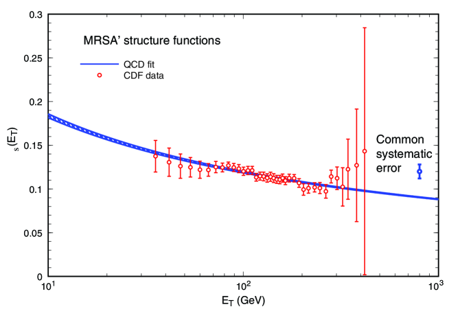
Figure 9: Values of $\alpha_{\rm s}(E_{T})$ extracted from CDF inclusive jet cross section data (figure adapted from [115]).

Giele, Glover and Yu determined $\alpha_{\rm s}$ [115] by fitting the NLO parton level Monte Carlo JETRAD [116], which is based on the QCD matrix elements of reference [117] and the MRSA’ parton density functions [118], to the single inclusive jet cross sections measured by CDF [119] for a cone size of $R=0.7$. In each bin of $E_{T}$, $\alpha_{\rm s}$ is determined for the scale choice $\mu\equiv E_{T}$. The resulting values of $\alpha_{\rm s}(E_{T})$ are displayed in figure 9, where the error bars represent the combined statistical and theoretical uncertainties; the size of an additional, overall (experimental) systematic error is also indicated. The results are in good agreement with the QCD expectation of the running $\alpha_{\rm s}$. A corresponding overall QCD fit, in NLO, gives

$$\alpha_{\rm s}(M_{\rm Z^{0}})=0.121\pm 0.001\ {\rm(stat.)}\pm 0.008\ {\rm(sys.)}\pm 0.005\ {\rm(theo.)}\ \pm 0.002\ {\rm(pdf)}\,$$

where the theoretical error was obtained from a variation of $\mu$ between 0.5 and $2\cdot E_{T}$, and the last error represents the uncertainty from using different parton density functions.

This study was basically meant to introduce a general method and possibility to determine $\alpha_{\rm s}$ from hadron collider jet cross sections, rather than to present a complete and final analysis. For instance, the parton density functions used in this study were extracted from (mainly deep inelastic scattering) data for a fixed input value of $\alpha_{\rm s}(M_{\rm Z^{0}})=0.113$, while a coherent determination of $\alpha_{\rm s}$ should allow $\alpha_{\rm s}$ to vary in the density functions, too. Although the data statistics — and hopefully also the experimental systematic errors — must have improved significantly with respect to the previous data sample of reference [119], and although there exist new parametrizations of density functions for different input values of $\alpha_{\rm s}$, no update of the measurement of $\alpha_{\rm s}$ from hadron collider jets was published so far. Therefore the above result is retained in the final summary — keeping in mind, however, that the quoted uncertainties constitute lower limits rather than a complete assessment of the overall error.

6 Results from heavy quarkonia decays and masses

The mass spectra and partial decay widths of heavy quark-antiquark bound states are a good testing ground for QCD. For quark masses $m_{Q}\gg\Lambda_{QCD}$, the short- and long-range effects on the decay widths can be factorized, and the short-range part can be calculated by perturbative QCD. Mass splittings of heavy quarkonia states can be calculated using nonperturbative methods like lattice gauge theory, which also provide means to extract values of $\alpha_{\rm s}$.

6.1 $\alpha_{\rm s}$ from quarkonia decay branching fractions

Partial decay widths of heavy quarkonia, like $\Gamma^{\mu\mu}=\Gamma(Q\overline{Q}\rightarrow\mu^{+}\mu^{-})$, $\Gamma^{\gamma gg}$ and $\Gamma^{ggg}$ are calculated in NLO QCD [120]. The expressions contain the (unknown) radial wave function at the origin, which can be eliminated by forming the ratios

$$R_{\mu} \equiv \frac{\Gamma^{ggg}}{\Gamma^{\mu\mu}}=\frac{10(\pi^{2}-9)}{9\pi}\frac{\alpha_{\rm s}^{3}(\mu^{2})}{\alpha^{2}}\left(1+\left[0.4-6.3\ln\left(\frac{m_{b}^{2}}{\mu^{2}}\right)\right]\frac{\alpha_{\rm s}(\mu^{2})}{\pi}\right)$$

$$R_{\gamma} \equiv \frac{\Gamma^{\gamma gg}}{\Gamma^{ggg}}=\frac{4}{5}\frac{\alpha}{\alpha_{\rm s}(\mu^{2})}\left(1-\left[2.6-2.1\ln\left(\frac{m_{b}^{2}}{\mu^{2}}\right)\right]\frac{\alpha_{\rm s}(\mu^{2})}{\pi}\right)\ .$$ (26)

An early, comprehensive fit of $\alpha_{\rm s}$ from the $J/\Psi$ and the $\Upsilon$ branching ratios was presented in reference [121], resulting in $\alpha_{\rm s}(M_{\rm Z^{0}})=0.113^{+0.007}_{-0.005}$. This study included estimates of the higher order QCD uncertainties and of relativistic corrections.

More recently, sum rules for the $\Upsilon$ system were analysed with resummation of QCD Coulomb effects which are responsible for the growth of the perturbative coefficients in NLO QCD [122], resulting in $\alpha_{\rm s}(M_{\rm Z^{0}})=0.118\pm 0.006$. Similar methods were already applied in ealier studies [123] but have led to conflicting results. Application of NNLO QCD predictions resulted in [124]

$$\alpha_{\rm s}(M_{\rm Z^{0}})=0.118\pm 0.006\ ,$$

which is included in the final summary of $\alpha_{\rm s}$. It should be noted that further studies of $\Upsilon$ sum rules in NNLO QCD [125] obtained similar results of $\alpha_{\rm s}$, however with a much more conservative estimate of the theoretical uncertainties — the resulting, large uncertainties of $\alpha_{\rm s}$ may indicate that $\Upsilon$ sum rules do not appear to provide competitive results of $\alpha_{\rm s}$.

6.2 $\alpha_{\rm s}$ from lattice calculations of mass splittings

Early determinations of $\alpha_{\rm s}$ from heavy quarkonia mass splittings were based on quenched approximations of lattice QCD calculations, neglecting light quark flavour loops ($N_{f}=0$). When evolved to the $\overline{\mbox{MS}}$ coupling at the scale $M_{\rm Z^{0}}$, these methods led to $\alpha_{\rm s}(M_{\rm Z^{0}})=0.105\pm 0.004$ [126], where the error included statistical as well as estimates of systematic errors.

Refined nonrelativistic QCD calculations with $N_{f}=0$ and $N_{f}=2$ allowed extrapolation to the physically correct number of light quarks, $N_{f}=3$, and included advanced (3-loop) perturbative extrapolation from the lattice to the $\overline{\mbox{MS}}$ coupling. A detailed study of various mass splittings of $\Upsilon$ ($b\overline{b}$) states, which are precisely known from corresponding measurements, was presented in [127]. Technically, the lattice calculation for a given value of the “bare” lattice coupling $\alpha_{lat}$ gave a value for the dimensionless quantity $a\Sigma$, where $a$ is the lattice spacing and $\Sigma$ is the mass splitting of suitable quarkonium states. From this result, divided by the measured value of $\Sigma$, the lattice spacing $a$ was obtained. From QCD perturbation theory, the $\overline{\mbox{MS}}$ coupling $\alpha_{\rm s}$ at the energy scale $a^{-1}$ is given as a function of $\alpha_{lat}$ [128]. Extraction of $\alpha_{\rm s}(a^{-1})$ and extrapolation to $\alpha_{\rm s}(M_{\rm Z^{0}})$ resulted in $\alpha_{\rm s}(M_{\rm Z^{0}})=0.1174\pm 0.0024$ [127], where the error included statistical as well as systematic uncertainties which include variations of light quark masses and estimates of truncation errors in the extraction of the $\overline{\mbox{MS}}$ coupling using perturbation theory.

More recently, a study based on similar lattice calculations and the same $\Upsilon$ mass splittings as in reference [127], however using a different discretization scheme, derived a lower value, $\alpha_{\rm s}(M_{\rm Z^{0}})=0.1118\pm 0.0017$ [129]. This is about three standard deviations smaller than the result from reference [127], which led to the conclusion that the “true” systematic uncertainty must be three to four times larger than estimated before.

Following this suggestion, the result on $\alpha_{\rm s}$ from nonperturbative lattice calculations to be considered in the final summary section is chosen to be the average of the two results discussed above, with the overall uncertainty increased by a factor of 3, giving

$$\alpha_{\rm s}(M_{\rm Z^{0}})=0.115\pm 0.006.$$

7 Summing up …

A summary of the $\alpha_{\rm s}$ measurements discussed in the previous sections is presented in table 6 at the end of this review. The results are given, if applicable, at the relevant energy scale $Q$ of the process, $\alpha_{\rm s}(Q)$, and at the standard “reference” scale of the $\rm Z^{0}$ mass, $\alpha_{\rm s}(M_{\rm Z^{0}})$. The conversion between these two cases was done [134] using the 4-loop QCD expression for the running $\alpha_{\rm s}$, equation 2.4, with 3-loop matching at the c- and b-quark pole masses of 1.5 and 4.7 GeV, respectively, as discussed in section 2.5. The splitting of the overall uncertainties of $\alpha_{\rm s}(M_{\rm Z^{0}})$, $\Delta\alpha_{\rm s}(M_{\rm Z^{0}})$, into experimental and theoretical errors is given in the $5^{th}$ and the $6^{th}$ columns of table 6, and the last column indicates the level of theoretical calculations on which these results are based.

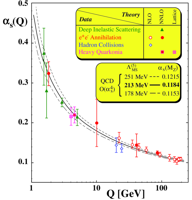
Figure 10: Summary of $\alpha_{\rm s}(Q)$ .

The results for $\alpha_{\rm s}(Q)$, given in the $3^{rd}$ column of table 6, are presented in figure 10, together with fits of the 4-loop QCD prediction for the running $\alpha_{\rm s}$ (equation 2.4) with 3-loop matching at the quark pole masses. Results which were obtained from data in large ranges of $Q$ are not displayed in this figure. The data are in very good agreement with the theoretical expectation, and prove the running of $\alpha_{\rm s}$ with high significance. The latter point will be analysed in more detail in section 7.2.

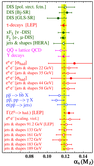
Figure 11: Summary of $\alpha_{\rm s}(M_{\rm Z^{0}})$ (filled symbols represent results based on complete NNLO QCD).

The values of $\alpha_{\rm s}(M_{\rm Z^{0}})$ are presented in figure 11. Within their assigned total erros, all results agree well with each other and with a weighted average value of $\alpha_{\rm s}(M_{\rm Z^{0}})=0.1184$, which is indicated by the vertical line in figure 11. The overall $\chi^{2}$ of all results with this average is 7.2 for 25 degrees of freedom, which indicates that the individual errors must be highly correlated. Therefore, the determination of the average value of $\alpha_{\rm s}(M_{\rm Z^{0}})$ and its overall uncertainty requires special treatment and discussion.

7.1 World average $\overline{\alpha_{\rm s}}(M_{\rm Z^{0}})$ and its overall uncertainty $\Delta\overline{\alpha_{\rm s}}$

The errors of most $\alpha_{\rm s}$ results are dominated by theoretical uncertainties, which are estimated using a variety of different methods and definitions. The significance of these nongaussian errors is largely unclear. Furthermore, there are large correlations between different results, due to common theoretical uncertainties, as e.g. for event shape measurements in ${\rm e^{+}\rm e^{-}}$ annihilations. Correlations between $\alpha_{\rm s}$ determinations from different processes, such as DIS and ${\rm e^{+}\rm e^{-}}$ annihilations, or between different procedures and observables used within the same class of processes may be present, too. Standard statistical methods therefore do not apply when averaging these results. Several methods are employed to derive an estimate of the average value $\overline{\alpha_{\rm s}}(M_{\rm Z^{0}})$ and its overall uncertainty, $\Delta\overline{\alpha_{\rm s}}$. The results are summarized in table 4:

• An error weighted average and an “optimized correlation” error is calculated from the error covariance matrix, assuming an overall correlation factor between the total errors of all measurements. This factor is adjusted so that the overall $\chi^{2}$ equals one per degree of freedom [130]. The resulting mean values, overall uncertainties and optimized correlation factors are given in columns 3 to 5 of Table 4, respectively.

• For illustrative purposes only, an overall error is calculated assuming that all measurements are entirely uncorrelated and all quoted errors are gaussian. The results are displayed in column 6.

• The simple, unweighted root mean squared of the mean values of all measurements is calculated and shown in column 7, labelled “simple rms”.

• Assuming that each result of $\alpha_{\rm s}(M_{\rm Z^{0}})$ has a rectangular-shaped rather than a gaussian probability distribution, the resulting weights (the inverse of the square of the total error) are summed up in a histogram, and the resulting $rms$ of that distribution is quoted as “rms box” [131].

All of these methods have certain advantages but also include inherent problems. The “simple rms” indicates the scatter of all results around their common mean, but does not depend on the individual errors quoted for each measurement. The “box rms”, which takes account of the errors and of their nongaussian nature, was criticized as being too conservative an estimate of the overall uncertainty of $\alpha_{\rm s}$. The “optimized correlation” method — in the absence of a detailed knowledge of these correlations — over-simplifies by the assumption of one overall correlation factor. Moreover, if correlations are present, $\chi^{2}$ does not have the same mathematical and probabilistic meaning as in the case of uncorrelated data. In the extreme, $\chi^{2}$ may even be negative.

Table 4: Average values of $\overline{\alpha_{\rm s}}(M_{\rm Z^{0}})$ and averaged uncertainties, for several methods to estimate the latter, and for several subsamples of the available data.

			opt. corr.	overall	uncorrel.	simple rms	rms box
row	sample (entries)	$\overline{\alpha_{\rm s}}(M_{\rm Z^{0}})$	$\Delta\overline{\alpha_{\rm s}}$	correl.	$\Delta\overline{\alpha_{\rm s}}$	$\Delta\overline{\alpha_{\rm s}}$	$\Delta\overline{\alpha_{\rm s}}$
1	all (26)	0.1191	0.0045	0.71	0.0012	0.0043	0.0057
2	$\Delta\alpha_{\rm s}\leq 0.010$ (20)	0.1191	0.0041	0.66	0.0012	0.0037	0.0051
3	$\Delta\alpha_{\rm s}\leq 0.008$ (18)	0.1190	0.0039	0.62	0.0012	0.0038	0.0050
4	$\Delta\alpha_{\rm s}\leq 0.006$ (9)	0.1188	0.0033	0.64	0.0014	0.0029	0.0038
5	$\Delta\alpha_{\rm s}\leq 0.005$ (4)	0.1189	0.0022	0.28	0.0017	0.0034	0.0033
6	NNLO only (9)	0.1185	0.0035	0.78	0.0016	0.0045	0.0048
7	$\Delta\alpha_{\rm s}\leq 0.008$ (6)	0.1184	0.0031	0.68	0.0016	0.0026	0.0032
8	$\Delta\alpha_{\rm s}\leq 0.005$ (3)	0.1184	0.0022	0.27	0.0018	0.0037	0.0028
9	$\Delta\alpha_{\rm s}\leq 0.004$ (2)	0.1175	0.0026	0.95	0.0019	0.0006	0.0019
10	only DIS (6)	0.1178	0.0040	0.94	0.0020	0.0014	0.0047
11	only ${\rm e^{+}\rm e^{-}}$ (15)	0.1209	0.0051	0.79	0.0016	0.0038	0.0054
12	only $p\overline{p}$ (3)	0.1135	0.0074	0.60	0.0051	0.0059	0.0068
13	$Q\leq 10$ GeV (9)	0.1177	0.0040	0.93	0.0016	0.0017	0.0042
14	$10<\frac{Q}{{\rm GeV}}<90$ (9)	0.1202	0.0064	0.56	0.0029	0.0062	0.0077
15	$Q\geq 90$ GeV (8)	0.1213	0.0056	0.78	0.0023	0.0035	0.0050

With these reservations in mind, all four methods do provide some estimate of $\Delta\overline{\alpha_{\rm s}}$. Apart from the method to calculate $\Delta\overline{\alpha_{\rm s}}$, the result also depends on the significance of the data included in the averaging process: in all cases except the “uncorrelated” error estimate, $\Delta\overline{\alpha_{\rm s}}$ is largest if all data are included, and tends to smaller values if the averaging is restricted to results with errors $\Delta\alpha_{\rm s}\leq\Delta\alpha_{\rm s}^{(max)}$, i.e. if only the most significant results are taken into account. This is demonstrated in rows 1 to 5 of table 4. The dependence of $\Delta\overline{\alpha_{\rm s}}$ on $\Delta\alpha_{\rm s}^{(max)}$ is illustrated in figure 12b, where the rightmost results correspond to the first row of table 4 which includes all 26 $\alpha_{\rm s}$ measurements summarized in table 6. Figure 12a illustrates the distribution of $\alpha_{\rm s}(M_{\rm Z^{0}})$ and the total errors of all these measurements.

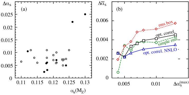
Figure 12: (a) Results of $\alpha_{\rm s}(M_{\rm Z^{0}})$ versus their respective overall errors; full symbols are based on complete NNLO QCD. (b) Dependence of $\Delta\overline{\alpha_{\rm s}}$ on the selection of results with errors $\Delta\alpha_{\rm s}(M_{\rm Z^{0}})\leq\Delta\alpha_{\rm s}^{(max)}$, for different methods to calculate $\overline{\alpha_{\rm s}}(M_{\rm Z^{0}})$. The rightmost data points correspond to no cut on $\Delta\alpha_{\rm s}^{(max)}$.

On first sight it seems logical to restrict the determination of $\overline{\alpha_{\rm s}}(M_{\rm Z^{0}})$, and especially of $\Delta\overline{\alpha_{\rm s}}$, to the most significant data, if the inclusion of less significant measurements only enlarges $\Delta\overline{\alpha_{\rm s}}$. Taken to the extreme, one may even be tempted to take the one result with the smallest quoted error as the final world average value of $\overline{\alpha_{\rm s}}(M_{\rm Z^{0}})$. However, the errors on $\alpha_{\rm s}(M_{\rm Z^{0}})$ estimated in individual studies are very often lower limits because unknown and additional systematic effects can only increase the total error. In some cases, small total errors can be due to fortunate coincidences, to ignorance, over-optimism and/or neglect of certain error sources. In order to ensure and to test consistency of the results, it is therefore mandatory not to rely on a single determination alone but to possibly include several different, significant measurements in the averaging process.

The averaging procedures discussed so far include results which are based on different orders and types of QCD calculations, namely on lattice gauge theory and on perturbation theory in NLO, resummed NLO and in NNLO. Comparing and averaging these different types of results is nevertheless justified because all of them include estimates of the relevant uncertainties, such that they should be compatible with a common average within their given errors. In order to achieve the highest precision and confidence in a combined average value $\overline{\alpha_{\rm s}}(M_{\rm Z^{0}})$, however, it may be beneficial not to include results which are, for instance, based on calculations in lower than the maximum available order of perturbation theory.

In this sense, the averaging procedure is applied only to those results which are based on complete NNLO QCD perturbation theory. Only very recently the number, the precision and the diversity of such measurements reached a level where such a restriction still provides a solid basis for a meaningful averaging process which includes sufficient freedom for internal consistency checks. Table 6 contains 9 measurements which are based on NNLO QCD; the results of averaging these are given in rows 6 to 9 of table 4, for different subsamples defined by selecting measurements with a total error $\Delta\alpha_{\rm s}\leq\Delta\alpha_{\rm s}^{(max)}$. The combined errors, $\Delta\overline{\alpha_{\rm s}}$, using the optimized correlation method, are displayed in figure 12b.

Requiring $\Delta\alpha_{\rm s}\leq 0.008$ rejects those $\alpha_{\rm s}$ measurements which are dominated by large experimental uncertainties, leaving the 5 most significant NNLO results from which one obtains, using the optimized correlation method,

$$\overline{\alpha_{\rm s}}(M_{\rm Z^{0}})=0.1184\pm 0.0031\ .$$

This value is taken as the currently best estimate of the world average of $\alpha_{\rm s}(M_{\rm Z^{0}})$. According to equations 2.4 and 8, in 4-loop approximation and with 3-loop threshold matching at $M_{b}=4.7$ GeV, this corresponds to $\Lambda_{\overline{\mbox{\scriptsize MS}}}^{(N_{f}=5)}=\left(213^{+38}_{-35}\right)$ MeV and $\Lambda_{\overline{\mbox{\scriptsize MS}}}^{(N_{f}=4)}=\left(296^{+46}_{-44}\right)$ MeV.

Each of the 26 single results summarized in table 6 is compatible with this average, to within about one standard deviation of its assigned uncertainty or less. In order to investigate possible systematic deviations or trends between and within subsets of these measurements, the averaging procedure was repeated for deep inelastic scattering data, for ${\rm e^{+}\rm e^{-}}$ annihilation and for hadron collider data alone, see rows 10 to 12 of table 4, and for 3 energy ranges as shown in rows 13 to 15. Within the overall uncertainties (e.g. those derived from the optimized correlation method), all results agree well with each other and with the world average value derived above. Small but insignificant systematic differences between DIS and ${\rm e^{+}\rm e^{-}}$ results and between those obtained from low and from high energy data may be visible; these may well be accidental or may be caused, for example, by different methods of treating renormalization and factorization scales.

7.2 Quantifying the running of $\alpha_{\rm s}$: determination of $\beta_{0}$, of $N_{c}$ and of the functional $Q$-dependence

The precision of the experimental results, the large energy range for which data are available, and the good agreement of the measurements with the QCD expectation of a running $\alpha_{\rm s}$, see figure 10, suggest actually fitting the functional form of the energy dependence from the data. For this purpose, a subset of data is selected which ensures maximal independence between the data chosen and which is based on the most significant measurements in the largest possible energy range (c.f. table 6 and figure 10), namely:

• $\alpha_{\rm s}$ from $\tau$ decays: $\alpha_{\rm s}(1.778\ {\rm GeV})=0.323\pm 0.030$;

• $\alpha_{\rm s}$ from moments of $F_{2}$: $\alpha_{\rm s}(2.96\ {\rm GeV})=0.252\pm 0.011$;

• $\alpha_{\rm s}$ from scaling violations of $F_{3}$: $\alpha_{\rm s}(5.0\ {\rm GeV})=0.214\pm 0.021$;

• $\alpha_{\rm s}$ from the hadronic width of the $\rm Z^{0}$: $\alpha_{\rm s}(91.2\ {\rm GeV})=0.124\pm 0.005$;

• $\alpha_{\rm s}$ from hadronic event shapes: $\alpha_{\rm s}(189\ {\rm GeV})=0.110\pm 0.004$.

All these results are based on complete NNLO QCD predictions — with the exception of the latter which includes resummed NLO calculations — and represent the most precise $\alpha_{\rm s}$ results of their class. The nature of their experimental and theoretical uncertainties ensures a maximum of independence between them.

Table 5: Functional fits of $\alpha_{\rm s}(Q^{2})$, in the energy range of $1.778~{}{\rm GeV}\leq Q\leq 189~{}{\rm GeV}$. The LO QCD expectation for $B\equiv 1/\beta_{0}$, with $N_{c}=3$ and $N_{f}=5$, is 1.64.

$\alpha_{\rm s}(Q)=...$	A	B	C	$\chi^{2}$ / d.o.f.	prob.
$B\left(\ln\frac{Q^{2}}{C^{2}}\right)^{-1}$	—	$1.62\pm 0.09$	$0.125\pm 0.032$	0.63 / 3	0.89
$A+C*Q$	$0.201\pm 0.007$	—	$(-5.3\pm 0.5)\cdot 10^{-4}$	78 / 3	$10^{-16}$
$A+C/Q$	$0.113\pm 0.003$	—	$0.41\pm 0.03$	4.6 / 3	0.20

Table 5 summarizes some of the functional fits which were performed with these selected data. The general idea was to obtain qualitative measures for the functional form of the energy dependence of $\alpha_{\rm s}$, as well as numeric fit values for the coefficient $\beta_{0}$ of the QCD $\beta$-function, see equation 3, and eventually for one of the main parameters of QCD, the number of colour degrees of freedom $N_{c}\equiv C_{A}$ which is an integral part of $\beta_{0}$:

$$\beta_{0}=\frac{11C_{A}-2N_{f}}{12\pi}\ .$$ (27)

Because of its simplicity and in order to avoid too many QCD-inspired biases, the functional form of the leading order QCD expression for the running $\alpha_{\rm s}$ ( c.f. equation 2.4), without quark threshold matching, was fitted to the data. Higher order corrections to the running affect $\alpha_{\rm s}$ at the smallest energy scales, $Q\sim M_{\tau}$, by less than $10\%$, which is well within the error of $\alpha_{\rm s}$ in this energy regime.

The results of this fit are given in the first row of table 5, with $B\equiv 1/\beta_{0}=1.62\pm 0.09$, and $C\equiv\Lambda=0.125\pm 0.032$ (in units of GeV). The $\chi^{2}$ of this fit is 0.63 for 3 degrees of freedom, which corresponds to a probability of 0.89. Within QCD, with $N_{c}=3$ and $N_{f}=5$, $1/\beta_{0}=1.64$, which is in excellent agreement with the fit value of the parameter $B$. $\Lambda=0.125$ GeV corresponds, in LO QCD, to $\alpha_{\rm s}(M_{\rm Z^{0}})=0.124$ and to $\alpha_{\rm s}(M_{\tau})=0.31$ (without threshold matching and with $N_{f}=5$ throughout). From the fit value of $B\equiv 1/\beta_{0}$ one can derive, according to equation 27 and for $N_{f}=5$ quark flavours,

$$N_{c}=3.03\pm 0.12\ ,$$

which is an excellent and precise verification of the QCD group structure which implies $N_{c}=3$. Alternatively, because this functional fit actually constrains the ratio $B/n$, where $n$ is the power of $Q/C$ inside the logarithm, the fit determines, when $B$ is fixed to its QCD value of 1.64, that $n=2.03\pm 0.12$.

Other functional forms of the energy dependence of $\alpha_{\rm s}$, which are not predicted by any consistent theory but which are added to demonstrate the significance of the logarithmic decrease of $\alpha_{\rm s}(Q^{2})$, are fitted and presented in the last two rows of table 5: a straight-line fit is clearly excluded by the unacceptable $\chi^{2}$ of 78 for 3 d.o.f., while a $1/Q$ energy dependence is disfavoured but cannot be excluded with the current data.

8 Conclusions

This review of experimental determinations of the coupling parameter of the Strong Interaction, $\alpha_{\rm s}$, summarized a topical and still ongoing field of activities in the high energy physics community. Due to impressive theoretical developments and experimental efforts during the past 10 years, $\alpha_{\rm s}$ could be determined from a large variety of physical observables and processes with steadily increasing precision. Current state-of-the-art measurements reach experimental uncertainties down to a few per cent, and theoretical calculations which are complete up to NNLO perturbative QCD obey higher order uncertainties of a few per cent in $\alpha_{\rm s}(M_{\rm Z^{0}})$, too. While not all of the available studies reach both these levels of precision, the most significant determinations of $\alpha_{\rm s}$, based on complete NNLO QCD calculations, can be summarized to a new world average value of

$$\overline{\alpha_{\rm s}}(M_{\rm Z^{0}})=0.1184\pm 0.0031\ .$$

The overall uncertainty is slightly larger than the smallest total errors quoted for some of the measurements, which is due to the following facts:

• The errors of single results contain different estimates of theoretical uncertainties, which are not uniquely defined.

• Many (if not all) results rely on assumptions which ultimately cannot be proven, like factorization between perturbative and nonperturbative effects, the nature and size of the latter, neglect of quark masses, exact realization of the electro-weak theory including the existence of a Standard Model Higgs boson, reaching of the continuum limit in lattice calculations etc.; the quoted theoretical uncertainties must therefore rather be viewed as lower limits instead of complete estimates.

• Many of the results and their theoretical uncertainties are highly correlated, however mostly to an unknown degree. This applies not only to their quoted errors, but also to the unproven assumptions mentioned under the previous item.

A realistic determination of the world average value of $\alpha_{\rm s}$ must therefore be based on comparing several different measurements of similar precision. It must account for possible correlations between them and allow for underestimates and fortunate cancellations of errors in some cases. In the absence of any “exact” method to account for all these effects, the “optimized correlation” method [130] was used to calculate the world average $\overline{\alpha_{\rm s}}(M_{\rm Z^{0}})$ and its overall remaining uncertainty as given above. The total error depends on the averaging method chosen - alternative procedures or preselections of data resulted in values ranging from $\pm 0.0022$ to $\pm 0.0057$.

All values of $\alpha_{\rm s}$ summarized in table 6 agree well, within their quoted uncertainties, with the world average. Averages obtained from various subsamples of these data, like those from deep inelastic scattering, from ${\rm e^{+}\rm e^{-}}$ annihilations and from hadron colliders, as well as subsamples from different energy ranges, do not show significant biases or shifts. In fact, the measured energy dependence of $\alpha_{\rm s}(Q^{2})$ is in excellent agreement with the QCD expectation and significantly proves the running of $\alpha_{\rm s}$.

Functional fits to data in the energy range from 1.78 to 189 GeV provide evidence for a logarithmic (in contrast to e.g. a linear) energy dependence, and the fitted logarithmic slope — if interpreted in terms of $\beta_{0}$, the LO coefficient of the QCD $\beta$-function — provides an accurate value for the number of colour degrees of freedom, $N_{c}=3.03\pm 0.12$. This is not actually a measurement of $N_{c}$, because many of the $\alpha_{\rm s}$ determinations are based on theoretical predictions of observables which inherently include the QCD value of $N_{c}=3$. Nevertheless, the fit result of $N_{c}$ from the measured energy dependence of $\alpha_{\rm s}$ constitutes an important consistency check between data and QCD.

The total uncertainty of $\overline{\alpha_{\rm s}}(M_{\rm Z^{0}})$ quoted above is $2.6\%$. This precision is a remarkable success. The error on $\overline{\alpha_{\rm s}}(M_{\rm Z^{0}})$, however, is much larger than those on other fundamental “constants” of nature, like the fine structure constant $\alpha$, the weak mixing angle $\sin^{2}\theta_{W}$ or the gravitational constant [5].

Any further reduction of the uncertainties on $\alpha_{\rm s}$ will require large theoretical as well as experimental efforts:

• New and higher order QCD calculations at least for some observables will be mandatory to understand, specify and possibly reduce theoretical uncertainties; most wishful candidates would be complete NNLO calculations for jet rates and hadronic event shapes in ${\rm e^{+}\rm e^{-}}$ annihilation and in DIS, which are well understood experimentally.

• The precision and theoretical understanding of parton density functions and their correlations with extracted values of $\alpha_{\rm s}$ must be significantly improved. Future high statistics and high energy runs of the Tevatron hadron collider will hopefully provide this important input. New theoretical developments to understand and predict structure functions from basic principles, for instance through application of classical string theory, see e.g. reference [132], are mandatory.

• So far, the neglect of finite (heavy) quark masses in almost all higher order QCD calculations potentially limits the reliability especially of results based on data which are close to these thresholds. While phase-space effects can be experimentally examined, only complete higher order QCD calculations for massive quarks, see e.g. reference [9], can close this gap of potentially large systematic uncertainties.

• The rôle of nonperturbative, long distance effects and the application of factorization in many processes and $\alpha_{\rm s}$ determinations must be further investigated and understood. Power corrections replacing or supplementing hadronization models, see e.g. references [84, 85], or higher twist corrections from lattice QCD, see e.g. reference [133], are promising new developments which have the potential for new, significant insights and improvements.

The physics of hadronic interactions at high energy colliders is rich and colourful. Much has been achieved in the past, however there are still many fundamental and open questions. Further and more precise determinations of the strong coupling parameter $\alpha_{\rm s}$ will continue to concern and employ many motivated scientists in the future.

Table 6: World summary of measurements of $\alpha_{\rm s}$ (DIS = deep inelastic scattering; GLS-SR = Gross-Llewellyn-Smith sum rule; Bj-SR = Bjorken sum rule; (N)NLO = (next-to-)next-to-leading order perturbation theory; LGT = lattice gauge theory; resum = resummed NLO).

	Q			$\Delta\alpha_{\rm s}(M_{\rm Z^{0}})$
Process	[GeV]	$\alpha_{s}(Q)$	$\alpha_{\rm s}(M_{\rm Z^{0}})$	exp.	theor.	Theory
DIS [pol. strct. fctn.]	0.7 - 8		$0.120\ ^{+\ 0.010}_{-\ 0.008}$	${}^{+0.004}_{-0.005}$	${}^{+0.009}_{-0.006}$	NLO
DIS [Bj-SR]	1.58	$0.375\ ^{+\ 0.062}_{-\ 0.081}$	$0.121\ ^{+\ 0.005}_{-\ 0.009}$	–	–	NNLO
DIS [GLS-SR]	1.73	$0.280\ ^{+\ 0.070}_{-\ 0.068}$	$0.112\ ^{+\ 0.009}_{-\ 0.012}$	${}^{+0.008}_{-0.010}$	$0.005$	NNLO
$\tau$-decays	1.78	$0.323\pm 0.030$	$0.1181\pm 0.0031$	0.0007	0.0030	NNLO
DIS [$\nu$; $x{\rm F_{3}}$]	5.0	$0.214\pm 0.021$	$0.118\pm 0.006$	$0.005$	$0.003$	NNLO
DIS [e/$\mu$; ${\rm F_{2}}$]	2.96	$0.252\pm 0.011$	$0.1172\pm 0.0024$	$0.0017$	$0.0017$	NNLO
DIS [e-p; jets]	6 - 100		$0.118\pm 0.011$	$0.002$	$0.011$	NLO
${\rm Q\overline{Q}}$ states	4.1	$0.216\pm 0.022$	$0.115\pm 0.006$	0.000	0.006	LGT
$\Upsilon$ decays	4.75	$0.22\pm 0.02$	$0.118\pm 0.006$	–	–	NNLO
${\rm e^{+}\rm e^{-}}$ [$\sigma_{\rm had}$]	10.52	$0.20\ \pm 0.06$	$0.130\ ^{+\ 0.021\ }_{-\ 0.029\ }$	$\ {}^{+\ 0.021\ }_{-\ 0.029\ }$	0.002	NNLO
${\rm e^{+}\rm e^{-}}$ [jets & shapes]	22.0	$0.161\ ^{+\ 0.016}_{-\ 0.011}$	$0.124\ ^{+\ 0.009}_{-\ 0.006}$	0.005	${}^{+0.008}_{-0.003}$	resum
${\rm e^{+}\rm e^{-}}$ [jets & shapes]	35.0	$0.145\ ^{+\ 0.012}_{-\ 0.007}$	$0.123\ ^{+\ 0.008}_{-\ 0.006}$	0.002	${}^{+0.008}_{-0.005}$	resum
${\rm e^{+}\rm e^{-}}$ [$\sigma_{\rm had}$]	42.4	$0.144\pm 0.029$	$0.126\pm 0.022$	$0.022$	0.002	NNLO
${\rm e^{+}\rm e^{-}}$ [jets & shapes]	44.0	$0.139\ ^{+\ 0.011}_{-\ 0.008}$	$0.123\ ^{+\ 0.008}_{-\ 0.006}$	0.003	${}^{+0.007}_{-0.005}$	resum
${\rm e^{+}\rm e^{-}}$ [jets & shapes]	58.0	$0.132\pm 0.008$	$0.123\pm 0.007$	0.003	0.007	resum
$\rm p\bar{\rm p}\rightarrow{\rm b\bar{b}X}$	20.0	$0.145\ ^{+\ 0.018\ }_{-\ 0.019\ }$	$0.113\pm 0.011$	${}^{+\ 0.007}_{-\ 0.006}$	${}^{+\ 0.008}_{-\ 0.009}$	NLO
${\rm p\bar{p},\ pp\rightarrow\gamma X}$	24.3	$0.135\ ^{+\ 0.012}_{-\ 0.008}$	$0.110\ ^{+\ 0.008\ }_{-\ 0.005\ }$	0.004	${}^{+\ 0.007}_{-\ 0.003}$	NLO
${\sigma(\rm p\bar{p}\rightarrow\ jets)}$	30 - 500		$0.121\pm 0.010$	0.008	0.005	NLO
${\rm e^{+}\rm e^{-}}$ [$\Gamma(\rm Z^{0}\rightarrow{\rm had.})$]	91.2	$0.124\pm 0.005$	$0.124\pm 0.005$	$0.004$	${}^{+0.003}_{-0.002}$	NNLO
${\rm e^{+}\rm e^{-}}$ scaling viol.	14 - 91.2		$0.125\pm 0.011$	${}^{+\ 0.006}_{-\ 0.007}$	0.009	NLO
${\rm e^{+}\rm e^{-}}$ [jets & shapes]	91.2	$0.121\pm 0.006$	$0.121\pm 0.006$	$0.001$	$0.006$	resum
${\rm e^{+}\rm e^{-}}$ [jets & shapes]	133.0	$0.113\pm 0.008$	$0.120\pm 0.007$	0.003	0.006	resum
${\rm e^{+}\rm e^{-}}$ [jets & shapes]	161.0	$0.109\pm 0.007$	$0.118\pm 0.008$	0.005	0.006	resum
${\rm e^{+}\rm e^{-}}$ [jets & shapes]	172.0	$0.104\pm 0.007$	$0.114\pm 0.008$	0.005	0.006	resum
${\rm e^{+}\rm e^{-}}$ [jets & shapes]	183.0	$0.109\pm 0.005$	$0.121\pm 0.006$	0.002	0.005	resum
${\rm e^{+}\rm e^{-}}$ [jets & shapes]	189.0	$0.110\pm 0.004$	$0.123\pm 0.005$	0.001	0.005	resum

References

-
[1]
H. Fritzsch, M. Gell-Mann and H. Leutwyler
Phys. Lett. B47 (1973) 365;
D.J. Gross, F. Wilczek, Phys. Rev. Lett. 30 (1973) 1343; Phys. Rev. D8 (1973) 3633;
H.D. Politzer, Phys. Rev. Lett. 30 (1973) 1346. - [2] R.K. Ellis, W.J. Stirling and B.R. Webber, QCD and Collider Physics, Cambridge University Press, 1996.
- [3] F.J. Yndurain, The Theory of Quark and Gluon Interactions, Ed., Springer-Verlag, 1999.
- [4] T. van Ritbergen, J.A.M. Vermaseren, S.A. Larin, Phys. Lett. B400 (1997) 379.
- [5] Review of Particle Properties, Eur. Phys. J. C3 (1998).
- [6] J.C. Collins, Renormalization, Cambridge University Press, 1984.
- [7] W.A. Bardeen et al., Phys. Rev. D18 (1978) 3998.
- [8] K.G. Chetyrkin, B.A. Kniehl and M. Steinhauser, Phys. Rev. Lett. 79 (1997) 2184.
-
[9]
W. Bernreuther, A. Brandenburg, P. Uwer, Phys. Rev. Lett. 79 (1997) 189;
G. Rodrigo, A. Santamaria, M. Bilenkii, Phys. Rev. Lett. 79 (1997) 193;
P. Nason, C. Oleari, Nucl. Phys. B521 (1998) 237. -
[10]
A.H. Hoang, J.H. Kühn, T. teubner, Nucl. Phys. B452 (1995) 173;
K.G. Chetyrkin, J.H. Kühn, M. Steinhauser, Nucl. Phys. B482 (1996) 213, Nucl. Phys. B505 (1997) 40. - [11] K.G. Chetyrkin, J.H. Kühn, Phys. Lett. B406 (1997) 102.
- [12] W. Bernreuther and W. Wetzel, Nucl. Phys. B197 (1982) 228.
- [13] S.A. Larin, T. van Ritbergen and J.A.M. Vermaseren, Nucl. Phys. B438 (1995) 278.
- [14] S. Catani, L. Trentadue, G. Turnock, B.R. Webber, Nucl. Phys. B407 (1993) 3.
- [15] The LEP Electroweak Working Group, CERN-EP/2000-016.
-
[16]
S.A.Larin, T. van Ritbergen, J.A.M. Vermaseren, Phys. Lett. B320 (1994) 159;
K.G. Chetyrkin, O.V. Tarasov, Phys. Lett. B327 (1994) 114. - [17] E. Tournefier, Proc. of the Quarks ’98 Int. Seminar, Suzdal, Russia, May 1998; hep-ex/9810042.
- [18] P.M. Stevenson, Phys. Rev. D23 (1981) 2916.
- [19] G. Grunberg, Phys. Rev. D29 (1984) 2315.
- [20] S.J. Brodsky, G.P. Lepage and P.B. Mackenzie, Phys. Rev. D28 (1983) 228.
-
[21]
G. Grunberg and A. Kataev, Phys. Lett. B279 (1992) 352;
J. Chyla, Phys. Lett. B356 (1995) 341;
L.R. Surguladze and M.A. Samuel, Rev. Mod. Phys. 68 (1996) 259;
C.J. Maxwell, hep-ph/9908463. - [22] S. Bethke, Z. Phys. C43 (1989), 331.
- [23] DELPHI Collaboration, P. Abreu et al., Z. Phys. C54 (1992) 55 .
- [24] OPAL Collaboration, P.D. Acton et al., Z. Phys. C55 (1992) 1.
- [25] DELPHI Collaboration, CERN-EP/99-133/revised, acc. by Eur. Phys. J. C.
- [26] P. Weisz, Nucl. Phys. B (Proc. Suppl.) 47 (1996) 71; hep-lat/9511017.
- [27] A. Gonzales-Arroyo, C. Lopez and F.J. Yndurain, Nucl. Phys. B153 (1979) 161.
-
[28]
V.N. Gribov and L.N. Lipatov, Sov. J. Nucl. Phys. 15 (1972) 438;
Yu.L. Dokshitzer, Sov. Phys. JETP 46 (1977) 641. - [29] G. Altarelli and G. Parisi, Nucl. Phys. B126 (1977) 298.
- [30] W. Furmanski and R. Petronzio, Z. Phys. C11 (1982) 293.
- [31] M. Virchaux and A. Milsztajn, Phys. Lett. B274 (1992) 221.
- [32] A.D. Martin, R.G Roberts and W.J. Stirling, Phys. Lett. B266 (1991) 173.
- [33] CCFR Collaboration, P.Z. Quintas et al., Phys. Rev. Lett. 71 (1993) 1307.
- [34] CCFR Collaboration, W.G. Seligman et al., Phys. Rev. Lett. 79 (1997) 1213.
- [35] R. Ball, S. Forte, Phys. Lett. B358 (1995) 365.
- [36] S. Alekhin, hep-ph/9907350.
- [37] S. Alekhin, hep-ph/9910490.
- [38] A.L. Kataev, G. Parente and A.V. Sidorov, hep-ph/9905310.
- [39] J. Santiago and F.J. Yndurain, Nucl. Phys. B(563) (1999) 45.
- [40] G. Altarelli, R.D. Ball, S. Forte and G. Ridolfi, Nucl. Phys. B496 (1997) 337; Acta Phys. Polon. B29 (1998) 1145.
- [41] D. Gross and C. Llewellyn Smith, Nucl. Phys. B14 (1969) 337.
- [42] J. Bjorken, Phys. Rev. D1 (1970) 1376.
- [43] J. Chyla and A.L. Kataev, Phys. Lett. B297 (1992) 385.
- [44] S.A. Larin, F.V. Tkachev and J.A.M. Vermaseren, Phys. Rev. Lett. 66 (1991) 862; S.A. Larin and J.A.M. Vermaseren, Phys. Lett. B259 (1991) 345.
- [45] CCFR Collaboration, W.C. Leung et al., Phys. Lett. B317 (1993) 655.
- [46] CCFR Collaboration, J.H. Kim et al., Phys. Rev. Lett. 81 (1998) 3595.
- [47] J. Ellis and M. Karliner, Phys. Lett B341 (1995) 397.
- [48] D. Adams et al., Phys. Lett. B329 (1994) 399.
- [49] E143 Collaboration, R. Arnold et al., Conf. on Intersections of Particle and Nuclear Physics, St. Petersburg, Florida, June 1994; Phys. Rev. Lett. 74 (1995) 346.
- [50] A.L. Kataev and V. Starshenko, CERN-TH-7198/94; hep-ph/9405294.
-
[51]
H1 Collaboration, T. Ahmed et al., Phys. Lett. B346 (1995) 415;
ZEUS Collaboration, M. Derrick et al., Phys. Lett. B363 (1995) 201;
H1 Collaboration, C. Adloff et al., Eur. Phys. J. C5 (1998) 625;
H1 Collaboration, C. Adloff et al., Eur. Phys. J. C6 (1999) 575. -
[52]
T. Brodkorb, J.G. Korner, E. Mirkes, G.A. Schuler, Z. Phys.
C44 (1989) 415;
D. Graudenz, Phys. Rev. D49 (1994) 3291. -
[53]
E. Mirkes and D. Zeppenfeld, Phys. Lett B380 (1996) 205;
S. Catani, M.H. Seymour, Nucl. Phys. B 485 (1997) 291. -
[54]
H1 Collaboration, C. Adloff et al., Phys. Lett. B406 (1997) 256;
H1 Collaboration, C. Adloff et al., hep-ex/9912052, acc. by Eur. Phys. J. C. - [55] M. Dasgupta, B.R. Webber, Eur. Phys. J. C1 (1998) 539; JHEP 9810 (1998) 1.
- [56] R.K. Ellis, D.A. Ross and A.E. Terrano, Nucl. Phys, B178 (1981) 421.
- [57] P. Nason and Z. Kunszt, in Z Physics at LEP-I, eds. G. Altarelli et al., CERN 89-08 (1989).
- [58] S. Catani, M.H. Seymour, Nucl. Phys. B485 (1997) 291; erratum ibid. B510 (1997) 503.
- [59] JADE Collaboration, W. Bartel et al., Phys. Lett. B119 (1982) 239.
- [60] S.L. Wu, Phys. Rep. 107 (1984) 59.
- [61] S. Bethke, Proc. of the Workshop on the Standard Model at the Energy of Present and Future Accelerators, June 1989, Budapest; LBL-28112 (1989).
- [62] S. Bethke and S. Catani, Proc. of the XXVIIth Rencontre de Moriond, Les Arcs, France, 1992; CERN-TH.6484/92.
- [63] G. Altarelli, Proc. of the “QCD – 20 Years Later” workshop at Aachen (1992), World Scientific; CERN-TH.6623/92.
- [64] T. Hebbeker, Phys. Rep. 217 (1992) 69.
- [65] S. Bethke and J. Pilcher, Ann. Rev. Nucl. Part. Sci. 42 (1992) 251.
- [66] S. Bethke, Proc. XXVI Int. Conf. on HEP, Dallas, Texas, August 1992; HD-PY 92/13.
- [67] S. Bethke, Z. Kunszt, D.E. Soper, W.J. Stirling, Nucl. Phys. B370 (1992) 310; erratum-ibid. B523 (1998) 681.
- [68] S. Bethke, Proc. Scottish Universities Summer School in Physics, August 1993, St. Andrews; HD-PY 93/7.
- [69] S. Bethke, Proc. Intern. Summer School on Particle Production Spanning MeV and TeV Energies, Nijmegen, Netherlands, 8-20 Aug 1999, MPI-PHE-2000-02, hep-ex/0001023.
-
[70]
S. Brandt et al., Phys. Lett. 12 (1964) 57;
E. Farhi, Phys. Rev. Lett. 39 (1977) 1587. -
[71]
JADE Collaboration, W. Bartel et al., Z. Phys. C33 (1986), 23;
JADE Collaboration, S. Bethke et al., Phys. Lett. B213 (1988), 235. - [72] S. Moretti, L. Lønnblad, T. Sjøstrand, JHEP 08 (1998) 1.
-
[73]
Yu. Dokshitzer, in Workshop on Jet Studies at LEP and HERA, Durham 1990;
see J. Phys. G17 (1991) 1572 ff;
N. Brown and W.J. Stirling, Z. Phys. C53 (1992) 629. -
[74]
P.A. Movilla Fernández et al., JADE Collaboration, Eur. Phys. J. C1
(1998) 461;
O. Biebel, P.A. Movilla-Fernandez, S. Bethke and the JADE Collaboration, Phys. Lett. B459 (1999) 326. - [75] TOPAZ Collaboration, Y. Ohnishi et al. Phys. Lett. B 313 (1993) 475.
-
[76]
ALEPH Collaboration, R. Barate et al., Phys. Rep. 294 (1998) 1;
CERN-OPEN-99-310 (1999); ALEPH-99-023. -
[77]
DELPHI Collaboration, P. Abreu et al., Phys. Lett B456 (1999) 322;
DELPHI-99-114. - [78] L3 Collaboration, M. Acciarri et al., Phys. Lett B444 (1998) 569; Phys. Lett. B404 (1997) 390; L3 note 2414.
- [79] OPAL Collaboration, G. Abbiendi et al., CERN-EP/99-178, subm. to Eur. Phys. J. C; Z. Phys. C75 (1997) 193; Z. Phys. C72 (1996) 191; Z. Phys. C59 (1993) 1.
- [80] SLD Collaboration, K. Abe et al., Phys. Rev. D51 (1995) 962.
-
[81]
L3 Collaboration, M. Acciarri et al., Phys. Lett B411 (1997) 339;
L3 note 2304 (1998). - [82] The JADE and the OPAL Collaborations, P. Pfeifenschneider et al., CERN-EP/99-175, hep-ex/0001055, subm. to Eur. Phys. J. C.
- [83] DELPHI Collaboration, CERN-EP/99-133, subm. to Eur. Phys. J. C.
-
[84]
Yu.L. Dokshitzer, B.R. Webber, Phys. Lett. B352 (1995) 451;
Yu.L. Dokshitzer, G. Marchesini, B.R. Webber, Nucl. Phys. B469 (1996) 93;
Yu.L. Dokshitzer, B.R. Webber, Phys. Lett. B404 (1997) 321;
S. Catani, B.R. Webber, Phys. Lett. B427 (1998) 377;
Yu.L. Dokshitzer, A. Lucenti, G. Marchesini, G.P. Salam, Nucl. Phys. B 511 (1998) 396; JHEP 05 (1998) 003. - [85] P.A. Movilla Fernández, O. Biebel, S. Bethke, hep-ex/9906033.
- [86] P. Nason, B.R. Webber, Nucl. Phys. B421 (1994) 473; Erratum-ibid. B480 (1996) 480.
- [87] J. Binnewies, hep-ph/9707269.
- [88] ALEPH Collaboration, D. Buskulic et al., Phys. Lett. B357 (1995) 487; Erratum-ibid. B364 (1995) 247.
- [89] DELPHI Collaboration, P. Abreu et al., Phys. Lett. B398 (1997) 194.
-
[90]
S.G. Gorishny, A.L. Kataev and S.A. Larin, Phys. Lett. 259B (1991) 144;
L.R. Surguladze and M.A. Samuel, Phys. Rev. Lett. 66 (1991) 560, Erratum ibid. 2416. - [91] K.G. Chetyrkin, Phys. Lett. B391 (1997) 402.
- [92] CELLO Collaboration, H. Behrend et al., Phys. Lett. B183 (1987) 400.
- [93] G. D’Agostini, W. de Boer and G. Grindhammer, Phys. Lett. B229 (1989) 160.
- [94] R. Marshall, Z. Phys. C43 (1989) 595.
- [95] D. Haidt, in Directions in High Energy Physics Vol 14, Precision Tests of the Standard Electroweak Model, ed. P. Langacker, World Scientific, 1995.
- [96] CLEO Collaboration, R. Ammar et al., Phys. Rev. D57 (1998) 1350.
-
[97]
A. Czarnecki, J. Kühn, Phys. Rev. Lett 77 (1996) 3955;
R. Harlander, T. Seidensticker, M. Steinhauser, Phys. lett. B426 (1998) 125. - [98] K.G. Chetyrkin, J.H. Kühn, A. Kwiatkowski, Physics report 277 (1996) 189.
- [99] A.L. Kataev, V.V. Starshenko, Mod. Phys. Lett. A10 (1995) 235.
- [100] E. Braaten, S. Narison and A. Pich, Nucl. Phys. B373 (1992) 581.
- [101] F. Le Diberder and A. Pich, Phys. Lett. B286 (1992) 147.
- [102] F. Le Diberder and A. Pich, Phys. Lett. B289 (1992) 165.
- [103] M.A. Shifman, L.A. Vainshtein, V.I. Zakharov, Nucl. Phys. B147 (1979) 385.
- [104] ALEPH Collaboration, R. Barate et al., Eur. Phys. J. C4 (1998) 409.
- [105] OPAL Collaboration, K. Ackerstaff et al., Eur. Phys. J C7 (1999) 571.
- [106] P. Ball, M. Beneke, V.M. Braun, Nucl. Phys. B452 (1995) 563.
- [107] M. Neubert, Nucl. Phys. B463 (1996) 511.
-
[108]
UA2 Collaboration, J. Alitti et al., Phys. Lett. B263 (1991) 563;
M. Lindgren et al., Phys. Rev. D45 (1992) 3038. - [109] D0 Collaboration, B. Abbott et al., FERMILAB-Conf-97/369-E.
- [110] UA1 Collaboration, C. Albajar et al., Phys. Lett. B369 (1996) 46.
- [111] M.L. Mangano, P. Nason, G. Ridolfi, Nucl. Phys. B373 (1992) 295.
- [112] P. Aurenche, R. Baier, M. Fontannaz, D. Schiff, Nucl. Phys. B297 (1988) 661.
- [113] UA6 Collaboration, M. Werlen et al., Phys. Lett. B452 (1999) 201.
- [114] J. Huth et al., in Research Directions for the Decade, ed. by E.L. Berger, World Scientific, Singapore, 1992.
- [115] W.T. Giele, E.W.N. Glover, J. Yu, Phys. Rev. D53 (1996) 120.
- [116] W.T. Giele, E.W.N. Glover, D.A. Kosower, Phys. Rev. Lett 73 (1994) 2019.
- [117] R.K. Ellis, J. Sexton, Nucl. Phys. B269 (1986) 445.
- [118] A.D. Martin, R.G. Roberts, W.J. Stirling, Phys. Rev. D50 (1994) 6734.
- [119] CDF Collaboration, F. Abe et al., Phys. Rev. Lett 68 (1992) 1104.
-
[120]
R. Barbieri, E. d’Emilio, G. Curci, E. Remiddi, Nucl. Phys. B154 (1979) 535;
P.B. Mackenzie, G.P. Lepage, Phys. Rev. Lett. 47 (1981) 1244;
P.B. Mackenzie, G.P. Lepage, in Proc. of Conf. on Pert. QCD, Tallahassee 1981; CLNS 81/498. - [121] M. Kobel, Proc. of the XXVII Rencontres de Moriond, Les Arcs, France, 1992.
- [122] J.H. Kühn, A.A. Penin and A.A. Pivovarov, Nucl. Phys. B534 (1998) 356.
-
[123]
M. Voloshin, Int. Jour. Mod. Phys. A10 (1995) 2865;
M. Jamin, A. Pich, Nucl. Phys. B507 (1997) 334. - [124] A. Penin, A.A. Pivovarov, Phys. Lett. B435 (1998) 413.
- [125] A.H. Hoang, Phys. Rev. D59 (1999), 014039; Phys. Rev. D61 (2000) 034005.
- [126] A.X. El-Khadra, G. Hockney, A.S. Kronfeld and P.B. Mackenzie, Phys. Rev. Lett. 69 (1992) 729.
- [127] C. Davies et al., Phys. Rev. D56 (1997) 2755; hep-lat/9706002.
-
[128]
B. Alles, M. Campostrini, A. Feo, H. Panagopoulos, Phys. Lett. B324 (1994)
433.
M. Luscher and P. Weisz, Phys. Lett B349 (1995) 165; Nucl. Phys. B452 (1995) 234. - [129] A. Spitz et al., Phys. Rev. D60 (1999) 074502.
- [130] M. Schmelling, Phys. Scripta 51 (1995) 676.
- [131] S. Bethke, Proc. QCD Euroconference 97, Montpellier, France, July (1997), Nucl. Phys. B (Proc.Suppl.) 64 (1998) 54; hep-ex/9710030.
- [132] D.E. Malov, A.S. Umar, D.J. Ernst, D.J. Dean, Phys. Rev. C 59 (1999) 2289.
- [133] S. Capitani et al., hep-ph/9906320.
- [134] A software package was developed to calculate and convert values of and of at different energy scales , performing automatic matching at the heavy quark flavour thresholds, incorporating equation 2.4 in 1- to 4-loop and up to 3-loop threshold matching according to equation 8. The program runs on Macintosh compatible computers and requires the “Hypercard” reader (version 2.0 or higher). It can be downloaded from http://home.cern.ch/~siggi/as4.Hqx .