Resonance structure of $\tau^{-}\to K^{-}\pi^{+}\pi^{-}\nu_{\tau}$ decays

Abstract

Using a sample of 4.7 fb^-1 integrated luminosity accumulated with the CLEO II detector at the Cornell Electron Storage Ring (CESR), we investigate the mass spectrum and resonant structure in $\tau^{-}\to K^{-}\pi^{+}\pi^{-}\nu_{\tau}$ decays. We measure the relative fractions of $K_{1}(1270)$ and $K_{1}(1400)$ resonances in these decays, as well as the $K_{1}$ masses and widths. Our fitted $K_{1}$ resonances are somewhat broader than previous hadroproduction measurements, and in agreement with recent LEP results from tau decay. The larger central value of our measured width supports models which attribute the small $\tau^{-}\to K^{-}\pi^{+}\pi^{-}\nu_{\tau}$ branching fraction to larger $K_{1}$ widths than are presently tabulated. We also determine the $K_{a}-K_{b}$ mixing angle $\theta_{K}$.

PACS numbers: 13.10+q, 13.35.Dx, 14.40.Aq

D. M. Asner,¹ A. Eppich,¹ J. Gronberg,¹ T. S. Hill,¹ D. J. Lange,¹ R. J. Morrison,¹ R. A. Briere,² B. H. Behrens,³ W. T. Ford,³ A. Gritsan,³ J. Roy,³ J. G. Smith,³ J. P. Alexander,⁴ R. Baker,⁴ C. Bebek,⁴ B. E. Berger,⁴ K. Berkelman,⁴ F. Blanc,⁴ V. Boisvert,⁴ D. G. Cassel,⁴ M. Dickson,⁴ P. S. Drell,⁴ K. M. Ecklund,⁴ R. Ehrlich,⁴ A. D. Foland,⁴ P. Gaidarev,⁴ R. S. Galik,⁴ L. Gibbons,⁴ B. Gittelman,⁴ S. W. Gray,⁴ D. L. Hartill,⁴ B. K. Heltsley,⁴ P. I. Hopman,⁴ C. D. Jones,⁴ D. L. Kreinick,⁴ M. Lohner,⁴ A. Magerkurth,⁴ T. O. Meyer,⁴ N. B. Mistry,⁴ C. R. Ng,⁴ E. Nordberg,⁴ J. R. Patterson,⁴ D. Peterson,⁴ D. Riley,⁴ J. G. Thayer,⁴ P. G. Thies,⁴ B. Valant-Spaight,⁴ A. Warburton,⁴ P. Avery,⁵ C. Prescott,⁵ A. I. Rubiera,⁵ J. Yelton,⁵ J. Zheng,⁵ G. Brandenburg,⁶ A. Ershov,⁶ Y. S. Gao,⁶ D. Y.-J. Kim,⁶ R. Wilson,⁶ T. E. Browder,⁷ Y. Li,⁷ J. L. Rodriguez,⁷ H. Yamamoto,⁷ T. Bergfeld,⁸ B. I. Eisenstein,⁸ J. Ernst,⁸ G. E. Gladding,⁸ G. D. Gollin,⁸ R. M. Hans,⁸ E. Johnson,⁸ I. Karliner,⁸ M. A. Marsh,⁸ M. Palmer,⁸ C. Plager,⁸ C. Sedlack,⁸ M. Selen,⁸ J. J. Thaler,⁸ J. Williams,⁸ K. W. Edwards,⁹ R. Janicek,¹⁰ P. M. Patel,¹⁰ A. J. Sadoff,¹¹ R. Ammar,¹² A. Bean,¹² D. Besson,¹² R. Davis,¹² I. Kravchenko,¹² N. Kwak,¹² X. Zhao,¹² S. Anderson,¹³ V. V. Frolov,¹³ Y. Kubota,¹³ S. J. Lee,¹³ R. Mahapatra,¹³ J. J. O’Neill,¹³ R. Poling,¹³ T. Riehle,¹³ A. Smith,¹³ J. Urheim,¹³ S. Ahmed,¹⁴ M. S. Alam,¹⁴ S. B. Athar,¹⁴ L. Jian,¹⁴ L. Ling,¹⁴ A. H. Mahmood,^14, M. Saleem,¹⁴ S. Timm,¹⁴ F. Wappler,¹⁴ A. Anastassov,¹⁵ J. E. Duboscq,¹⁵ K. K. Gan,¹⁵ C. Gwon,¹⁵ T. Hart,¹⁵ K. Honscheid,¹⁵ D. Hufnagel,¹⁵ H. Kagan,¹⁵ R. Kass,¹⁵ T. K. Pedlar,¹⁵ H. Schwarthoff,¹⁵ J. B. Thayer,¹⁵ E. von Toerne,¹⁵ M. M. Zoeller,¹⁵ S. J. Richichi,¹⁶ H. Severini,¹⁶ P. Skubic,¹⁶ A. Undrus,¹⁶ S. Chen,¹⁷ J. Fast,¹⁷ J. W. Hinson,¹⁷ J. Lee,¹⁷ N. Menon,¹⁷ D. H. Miller,¹⁷ E. I. Shibata,¹⁷ I. P. J. Shipsey,¹⁷ V. Pavlunin,¹⁷ D. Cronin-Hennessy,¹⁸ Y. Kwon,^18, A.L. Lyon,¹⁸ E. H. Thorndike,¹⁸ C. P. Jessop,¹⁹ H. Marsiske,¹⁹ M. L. Perl,¹⁹ V. Savinov,¹⁹ D. Ugolini,¹⁹ X. Zhou,¹⁹ T. E. Coan,²⁰ V. Fadeyev,²⁰ Y. Maravin,²⁰ I. Narsky,²⁰ R. Stroynowski,²⁰ J. Ye,²⁰ T. Wlodek,²⁰ M. Artuso,²¹ R. Ayad,²¹ C. Boulahouache,²¹ K. Bukin,²¹ E. Dambasuren,²¹ S. Karamov,²¹ S. Kopp,²¹ G. Majumder,²¹ G. C. Moneti,²¹ R. Mountain,²¹ S. Schuh,²¹ T. Skwarnicki,²¹ S. Stone,²¹ G. Viehhauser,²¹ J.C. Wang,²¹ A. Wolf,²¹ J. Wu,²¹ S. E. Csorna,²² I. Danko,²² K. W. McLean,²² Sz. Márka,²² Z. Xu,²² R. Godang,²³ K. Kinoshita,^23, I. C. Lai,²³ S. Schrenk,²³ G. Bonvicini,²⁴ D. Cinabro,²⁴ L. P. Perera,²⁴ G. J. Zhou,²⁴ G. Eigen,²⁵ E. Lipeles,²⁵ M. Schmidtler,²⁵ A. Shapiro,²⁵ W. M. Sun,²⁵ A. J. Weinstein,²⁵ F. Würthwein,^25, D. E. Jaffe,²⁶ G. Masek,²⁶ H. P. Paar,²⁶ E. M. Potter,²⁶ S. Prell,²⁶ and V. Sharma²⁶

I Introduction

Decays of the $\tau$ lepton into three pseudoscalars have been actively studied over the last several years. Lately, a number of relatively precise measurements of the branching fractions for $\tau^{-}\to K^{-}\pi^{+}\pi^{-}\nu_{\tau}$ have become available from the ALEPH, CLEO and OPAL collaborations[1, 2, 3, 4]. However, the resonance substructure of these decays has not yet been measured with high precision.

The decay $\tau^{-}\to K^{-}\pi^{+}\pi^{-}\nu_{\tau}$, with its simple and well-understood initial state provides information on low-$Q^{2}$ QCD. The effects of $SU(3)_{f}$ symmetry breaking can be observed, the decay constants of the $K_{1}$ resonances can be measured, and the hadronic resonance substructure can be studied from an analysis of the final state invariant mass spectra [5, 6]. Other interesting topics include resonance parameters (such as the widths of the $K_{1}$ states), tests of isospin relations, and measurements of the Wess-Zumino anomaly. Current models of this decay [7, 8] are based on Chiral Perturbation Theory (ChPT) calculations. The question of the $K_{1}$ widths is of special interest because the theoretical models based on ChPT [8] provide predictions for the $\tau^{-}\to K^{-}h^{+}h^{-}\nu_{\tau}$ branching fractions that are significantly larger than current experimental values[2, 3]. This discrepancy can be resolved if the $K_{1}$ resonances in $\tau$ decays are much wider than presently measured values. In the non-strange sector, it has long been realized that the $a_{1}$ width is considerably larger as measured in $\tau^{-}\to a_{1}^{-}\nu_{\tau}$ compared to hadronic production of the $a_{1}$. The primary goal of this analysis is to measure the relative amplitudes of the $K_{1}(1270)$ and $K_{1}(1400)$ resonances that are believed to dominate $\tau^{-}\to K^{-}\pi^{+}\pi^{-}\nu_{\tau}$ decays[7, 8] and to determine the parameters of the $K_{1}$ resonances.

II Theoretical aspects of $\tau^{-}\to K^{-}\pi^{+}\pi^{-}\nu_{\tau}$ decays

In the Standard Model, the general form for the semileptonic $\tau$-decay matrix element can be written [9] as

$${\cal M}=\frac{G}{\sqrt{2}}\bar{u}(p_{\nu})\gamma^{\mu}(1-\gamma_{5})u(p_{\tau})J_{\mu},$$ (1)

where $J_{\mu}\equiv\langle K\pi\pi|V_{\mu}-A_{\mu}|0\rangle$ is the hadronic current and $p_{\nu}$ and $p_{\tau}$ are the four-momenta of the $\tau$ neutrino and the $\tau$ lepton, respectively.

General considerations based on Lorentz invariance and conservation of energy and momentum lead to the conclusion that only four independent form-factors are needed to describe the hadronic current in $\tau^{-}\to K^{-}\pi^{+}\pi^{-}\nu_{\tau}$. One parameterization[7, 8] describes this process as

$$J^{\mu}= [F_{1}(s_{1},s_{2},Q^{2})(p_{2}-p_{3})_{\nu}+F_{2}(s_{1},s_{2},Q^{2})(p_{1}-p_{3})_{\nu}]T^{\mu\nu}$$ (2)

$$+F_{a}(s_{1},s_{2},Q^{2})\epsilon^{\mu\nu\rho\sigma}p_{1\nu}p_{2\rho}p_{3\sigma}+F_{s}(s_{1},s_{2},Q^{2})Q^{\mu},$$ (3)

where $F_{i}$ are form-factors, $Q^{\mu}$ is the $K\pi\pi$ 4-vector, $s_{1}$ is expressed in terms of the final state hadrons’ momenta $p_{i}$ ($i$=1 for the $K^{-}$, $i$=2 for $\pi^{+}$ and $i$=3 for $\pi^{-}$) as $s_{1}=(p_{2}+p_{3})^{2}$, $s_{2}=(p_{1}+p_{3})^{2}$ and $T^{\mu\nu}=(g^{\mu\nu}-Q^{\mu}Q^{\nu}/Q^{2})$. Here, there are two axial vector form-factors $F_{1}$ and $F_{2}$, an anomalous vector form-factor $F_{a}$, and a scalar form-factor $F_{s}$.

To derive specific expressions for the form-factors, some assumptions have to be made. It is believed [7, 8] that this decay is dominated by the lowest-mass resonances. There are two axial vector resonances which can produce the $K^{-}\pi^{+}\pi^{-}$ final state. These are the weak eigenstates ${}^{3}P_{1}$ and ${}^{1}P_{1}$ $(u\bar{s})$, called $K_{a}$ and $K_{b}$. The $K_{b}$ couples to the $W$ analagous to a “second class” current, violating $SU(3)_{f}$ symmetry. These two weak eigenstates mix with mixing angle $\theta_{K}$ to form the observable mass eigenstates, $K_{1}(1270)$ and $K_{1}(1400)$ [5]. The $K_{1}(1270)$ subsequently decays into $K^{*}\pi$, $K\rho$ or $K\rho^{\prime}$, while the $K_{1}(1400)$ decays almost entirely to $K^{*}\pi$.

Within the context of ChPT, the form-factors can be written[8] as

$$F_{1}=\frac{\sqrt{2}}{3}\cdot BW_{K_{1}(1270)}\frac{BW_{\rho}+\xi BW_{\rho^{\prime}}}{1+\xi}$$ (4)

$$F_{2}=-\frac{\sqrt{2}}{3}\cdot\frac{\eta BW_{K_{1}(1270)}+BW_{K_{1}(1400)}}{(1+\eta)}\cdot BW_{K^{*}},$$ (5)

where $BW$ denotes a Breit-Wigner mass distribution. The parameter $\eta$ is estimated to be 0.33 in [8]. The coefficients preceding the Breit-Wigner expressions are fixed by ChPT. In the first form-factor, the coefficient $\xi$ is taken to be -0.145 based on application of the Conserved Vector Current (CVC) to $e^{+}e^{-}\to\pi^{+}\pi^{-}$ data [8, 10].

In the chiral limit, the scalar form-factor $F_{s}$ is zero. The vector form-factor $F_{a}$ is expected to be numerically small compared to $F_{1}$ and $F_{2}$; it is only non-zero due to the Wess-Zumino anomaly. The vector contribution is approximately $5.5\%$ as calculated using the decay amplitudes found in [9]. For this analysis, we will assume that the vector contribution is zero, and include our uncertainty in this term as a systematic error.

ChPT has found widespread application in tau decays. A model similar to this is used for our analysis of the invariant mass distributions in $\tau^{-}\to K^{-}\pi^{+}\pi^{-}\nu_{\tau}$, as will be described in the following sections.

III Data sample and event selection

Our data sample contains approximately 4.3 million $\tau$-pairs produced in $e^{+}e^{-}$ collisions, corresponding to an integrated luminosity of 4.7 fb^-1. The data were collected with the CLEO II detector[11] at the Cornell Electron Storage Ring, operating at a center-of-mass energy approximately 10.58 GeV.

The CLEO II detector is a general-purpose solenoidal magnet spectrometer and calorimeter. The detector was designed for efficient triggering and reconstruction of two-photon, tau-pair, and hadronic events. Measurements of charged particle momenta are made with three nested coaxial drift chambers consisting of 6, 10, and 51 layers, respectively. These chambers fill the volume from $r$=3 cm to $r$=1 m, with $r$ the radial coordinate relative to the beam (${\hat{z}}$) axis. This system is very efficient ($\epsilon\geq$98%) for detecting tracks that have transverse momenta ($p_{T}$) relative to the beam axis greater than 200 MeV/$c$, and that are contained within the good fiducial volume of the drift chamber ($|\cos\theta|<$0.94, with $\theta$ defined as the polar angle relative to the beam axis). This system achieves a momentum resolution of $(\delta p/p)^{2}=(0.0015p)^{2}+(0.005)^{2}$ ($p$ is the momentum, measured in GeV/$c$). Pulse-height measurements in the main drift chamber provide specific ionization ($dE/dx$) resolution of 5.5% for Bhabha events, giving good $K/\pi$ separation for tracks with momenta up to 700 MeV/$c$ and nearly 2$\sigma$ separation in the relativistic rise region above 2 GeV/$c$. Outside the central tracking chambers are plastic scintillation counters, which are used as a fast element in the trigger system and also provide particle identification information from time-of-flight measurements.

Beyond the time-of-flight system is the electromagnetic calorimeter, consisting of 7800 thallium-doped CsI crystals. The central “barrel” region of the calorimeter covers about 75% of the solid angle and has an energy resolution which is empirically found to follow:

$$\frac{\sigma_{\rm E}}{E}(\%)=\frac{0.35}{E^{0.75}}+1.9-0.1E;$$ (6)

$E$ is the shower energy in GeV. This parameterization includes effects such as noise, and translates to an energy resolution of about 4% at 100 MeV and 1.2% at 5 GeV. Two end-cap regions of the crystal calorimeter extend solid angle coverage to about 95% of $4\pi$, although energy resolution is not as good as that of the barrel region. The tracking system, time of flight counters, and calorimeter are all contained within a superconducting coil operated at 1.5 Tesla. Flux return and tracking chambers used for muon detection are located immediately outside the coil and in the two end-cap regions.

We select $e^{+}e^{-}\to\tau^{+}\tau^{-}$ events having a 1-prong vs. 3-prong topology in which one $\tau$ lepton decays into one charged particle (plus possible neutrals), and the other $\tau$ lepton decays into 3 charged hadrons (plus possible neutrals). An event is separated into two hemispheres based on the measured event thrust axis. Loose cuts on ionization measured in the drift chamber, energy deposited in the calorimeter and the maximum penetration depth into the muon detector system are applied to charged tracks in the signal (3-prong) hemisphere to reject leptons. Backgrounds from non-signal $\tau$ decays and hadronic events with $K_{S}^{0}$ are suppressed by requirements on the impact parameters of charged tracks. To reduce the background from two-photon collisions ($e^{+}e^{-}\to e^{+}e^{-}\gamma\gamma$ with $\gamma\gamma\to$hadrons or $\gamma\gamma\to l^{+}l^{-}$), cuts on visible energy ($E_{vis}$) and total event transverse momentum ($P_{t}$) are applied: $2.5$ GeV $<E_{vis}<10$ GeV, and $P_{t}>$0.3 GeV/$c$. We also require the invariant mass of the tracks and showers in the 3-prong hemisphere, calculated under the $\pi^{-}\pi^{+}\pi^{-}$ hypothesis, to be less than 1.7 GeV/$c$. Events are accepted for which the tag hemisphere (1-prong side) is consistent with one of the following four decays: $\tau^{+}\rightarrow e^{+}\nu_{e}{\overline{\nu}_{\tau}}$, $\tau^{+}\rightarrow\mu^{+}\nu_{\mu}{\overline{\nu}_{\tau}}$, $\tau^{+}\rightarrow\pi^{+}{\overline{\nu}_{\tau}}$, or $\tau^{+}\rightarrow\rho^{+}{\overline{\nu}_{\tau}}$.

Candidate events are distinguished from background $\tau$ decays with $\pi^{0}$’s and continuum hadronic background ($e^{+}e^{-}\to q\bar{q}$) by the characteristics of showers in the electromagnetic calorimeter. A photon candidate is defined as a shower in the barrel region of the electromagnetic calorimeter with energy above 100 MeV having an energy deposition pattern consistent with true photons. It must be separated from the closest charged track by at least 30 cm. $\tau^{-}\to K^{-}\pi^{+}\pi^{-}\nu_{\tau}$ candidates are defined as those events having zero photon candidates in the 3-prong hemisphere.

The event selection described above provides a sample of events that contains $\tau^{-}\to\pi^{-}\pi^{+}\pi^{-}\nu_{\tau}$, $\tau^{-}\to K^{-}\pi^{+}\pi^{-}\nu_{\tau}$ and $\tau^{-}\to K^{-}K^{+}\pi^{-}\nu_{\tau}$. In this analysis we neglect possible contributions from the decays $\tau^{-}\rightarrow\pi^{-}K^{+}\pi^{-}\nu_{\tau}$ and $\tau^{-}\rightarrow K^{-}\pi^{+}K^{-}\nu_{\tau}$ because they are unphysical in the Standard Model and have not been experimentally observed. We also neglect the $\tau^{-}\rightarrow K^{-}K^{+}K^{-}\nu_{\tau}$ final state. This rate is expected to be $\sim 1\%$ relative to that for $\tau^{-}\rightarrow K^{-}\pi^{+}\pi^{-}\nu_{\tau}$ due to the limited phase space and the low probability of forming an $(s\bar{s})$ pair from the vacuum.

IV Reconstruction of invariant mass spectra

Due to the very small fraction of kaons in $\tau^{-}\to h^{-}h^{+}h^{-}\nu_{\tau}$ events and the limited particle identification capabilities of the CLEO II detector, it is difficult to identify individual $\tau^{-}\to K^{-}\pi^{+}\pi^{-}\nu_{\tau}$ decays. In this analysis, a statistical approach is used in which the number of $\tau^{-}\to K^{-}h^{+}\pi^{-}\nu_{\tau}$ events in any given sample is determined using the $dE/dx$ information of the two same-sign tracks in the signal hemisphere. The $dE/dx$ analysis is described in detail in [3].

For each $h^{-}h^{+}h^{-}$ candidate the invariant mass of the three hadrons is calculated under two hypotheses for the first and the third tracks, corresponding to the $K^{-}\pi^{+}\pi^{-}$ and $\pi^{-}\pi^{+}K^{-}$ mass assignments. Each of these two sub-samples is divided into bins of invariant mass. The bins are 100 MeV/$c^{2}$ wide, spanning the region $0.8-1.7$ GeV/$c^{2}$. After binning in mass, the sub-samples that correspond to the same mass bin are combined.

The $dE/dx$ analysis provides the number of kaons in each mass bin, which is equal to the number of $\tau^{-}\to K^{-}h^{+}\pi^{-}\nu_{\tau}$ events in that mass interval. The invariant mass spectrum of the $K^{-}\pi^{+}\pi^{-}$ system is thereby reconstructed. This distribution contains a contribution from $\tau^{-}\to K^{-}K^{+}\pi^{-}\nu_{\tau}$ decays which must be subtracted, as will be discussed in Sec.V.

In a similar way the invariant mass spectra of $K^{-}\pi^{+}$ and $\pi^{+}\pi^{-}$ are reconstructed in ten bins over the range $0.5$ GeV/$c^{2}<M_{K^{-}\pi^{+}}<1.5$ GeV/$c^{2}$ and $0.2$ GeV/$c^{2}<M_{\pi^{+}\pi^{-}}<1.2$ GeV/$c^{2}$, respectively. The reconstructed mass spectra are shown in Fig. 1.

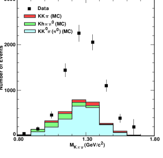
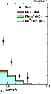
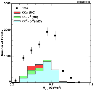
FIG. 1.: Reconstructed mass spectra (data) and backgrounds predicted from Monte Carlo simulations.

V Background and efficiency

There are two main types of background: continuum hadronic events ($e^{+}e^{-}\to q\bar{q}\to hadrons$) and non-signal $\tau$ decays. Hadronic background is estimated from a continuum hadronic Monte Carlo sample (using the JETSET v7.3 [12] event generator and GEANT[13] detector simulation code). This background is subtracted as described in [3]. The level of hadronic background is approximately 3%.

$\tau$-related background comes primarily from $\tau^{-}\to K^{-}K^{+}\pi^{-}\nu_{\tau}$ decays. These events comprise approximately $27\%$ of the events in our reconstructed invariant mass distributions. Smaller background contributions arise from $\tau^{-}\to K^{-}h^{+}\pi^{-}\pi^{0}\nu_{\tau}$ with incomplete $\pi^{0}$ reconstruction and also tau decays to the $K^{-}\pi^{+}\pi^{-}(\pi^{0})\nu_{\tau}$ final state through an intermediate $K^{0}_{S}$. These two backgrounds comprise 5% and 3% of the events in the $K^{-}\pi^{+}\pi^{-}$ invariant mass spectra, respectively. The invariant mass distributions for backgrounds are found using Monte Carlo simulations to obtain the shape; the normalization is set by the measured branching fractions [3, 14]. Background predictions are shown in Fig. 1. The invariant mass distributions for all backgrounds are subtracted from the corresponding invariant mass spectra reconstructed from data.

The efficiency of event reconstruction depends slightly on the invariant mass. Therefore, it is necessary to introduce a mass-dependent efficiency correction. This correction is calculated from $\tau$ Monte Carlo using the KORALB event generator [9]. The maximum variation in efficiency across the mass interval of interest is of order 10%.

VI Fitting method

The hadronic structure of the $K^{-}\pi^{+}\pi^{-}$ system is investigated by simultaneously fitting three invariant mass distributions: $M_{K^{-}\pi^{+}\pi^{-}}$, $M_{K^{-}\pi^{+}}$ and $M_{\pi^{+}\pi^{-}}$. The fitting function is based upon a model similar to the one described in Sec. I, and now outlined in greater detail.

A Parameterization of form-factors

In this analysis, we write the following expression for the axial vector form-factors $F_{1}$ and $F_{2}$:

$$F_{1}=\frac{1}{\sqrt{3}}(A\cdot BW_{1270}+B\cdot BW_{1400})\frac{BW_{\rho}+\xi BW_{\rho^{\prime}}}{1+\xi}$$ (7)

$$F_{2}=(-\frac{2}{3})(C\cdot BW_{1270}+D\cdot BW_{1400})BW_{K^{*}}$$ (8)

that contain the four real parameters $A-D$. Of these, 3 are independent; the fourth is fixed by the normalization requirement that the squared sum of the $\tau^{-}\to K_{1}^{-}(1270)\nu_{\tau}$ and $\tau^{-}\to K_{1}^{-}(1400)\nu_{\tau}$ amplitudes must saturate the total $\tau^{-}\to K^{-}\pi^{+}\pi^{-}\nu_{\tau}$ rate. The coefficients $A$ and $B$ correspond to production of the $K\rho$ final state through either $K_{1}$(1270) ($A$) or $K_{1}$(1400) ($B$), modulo a factor which includes the appropriate phase space weighting for various final states (denoted as “$R_{A}$”, or “$R_{B}$”). In our analysis, we fix $B$ to be zero, consistent with current measurements [14]. Similarly, $C$ and $D$ designate production of the $K^{*}\pi$ final state through the $K_{1}(1270)$ and $K_{1}(1400)$ resonances. The decay amplitude parameters in Eqs. (7)-(8) therefore correspond to the possible decay chains as

$$\tau\to K_{1}(1270)\nu\to K\rho\nu\to K^{-}\pi^{+}\pi^{-}\nu_{\tau}: ``A^{\prime\prime}$$ (9)

$$\tau\to K_{1}(1270)\nu\to K^{*}\pi\nu\to K^{-}\pi^{+}\pi^{-}\nu_{\tau}: ``C^{\prime\prime}= A\cdot\sqrt{\frac{16}{42}}\cdot{\sqrt{\frac{R_{A}}{R_{C}}}}$$ (10)

$$\tau\to K_{1}(1400)\nu\to K^{*}\pi\nu\to K^{-}\pi^{+}\pi^{-}\nu_{\tau}: ``D^{\prime\prime}= \sqrt{1-A^{2}-C^{2}}$$ (11)

In Eqs. (9)-(10) we have imposed constraints that follow from the tabulated branching fractions of the $K_{1}$ resonances [14]: ${\cal B}({K_{1}(1270)\to K^{*}\pi})=(16\pm 5)$% and ${\cal B}({K_{1}(1270)\to K\rho})=(42\pm 6)$%.

Thus, in our parameterization of the matrix element one unknown parameter $A$ defines all four amplitudes. In addition, the masses and widths of the $K_{1}$ resonances $\Gamma_{K_{1}(1270)}$, $\Gamma_{K_{1}(1400)}$, $M_{K_{1}(1270)}$, $M_{K_{1}(1400)}$ are considered unknown and left as free parameters in the fit. The Breit-Wigner distributions for the $K_{1}$ resonances are defined following the approach of [9] as

$$BW(s,m_{K_{1}},\Gamma_{K_{1}})=\frac{m_{K_{1}}^{2}-im_{K_{1}}\Gamma_{K_{1}}}{m_{K_{1}}^{2}-s-im_{K_{1}}\Gamma_{K_{1}}}\;\;.$$ (12)

The Breit-Wigner distributions for the $K^{*}$ and $\rho$ resonances contain mass-dependent widths:

$$BW(s,m,\Gamma)=\frac{m^{2}}{m^{2}-s-i\sqrt{s}\Gamma(s)},$$ (13)

where the mass-dependence is defined by Eq. (22) in [9]:

$$\Gamma(s)=\Gamma_{0}\frac{m_{0}^{2}}{s}\left(\frac{p(s)}{p(m_{0}^{2})}\right)^{\frac{3}{2}}.$$ (14)

Here, $m_{0}$ and $\Gamma_{0}$ are the nominal mass and width of a particle, $p$ is the momentum of the particle, and the variable $s$ is the three- or two-body invariant mass, as appropriate.

The constants $R_{X}$ (where $X=A,...,D$) in Eqs. (9), (10), and (11) depend on the masses and widths of the 2- and 3-body resonances in this decay and are calculated by numerical integration of the appropriate matrix element. Since we are interested in the ratios of quantities (e.g., branching fractions), the overall normalization of the $R_{X}$ parameters is arbitrary.

In this analysis, we have determined the numerical coefficients for the Breit-Wigner terms [$\sqrt{\frac{1}{3}}$ and $-\frac{2}{3}$ in Eqs. (7)-(8)] using isospin relations rather than taking the chiral limit as in [8]. The Wess-Zumino anomaly term is set to zero in our model; this term is numerically small enough that it can be neglected at our level of accuracy. Appropriate systematic errors are assigned to reflect the possible magnitude of this contribution. Note, however, that if the Wess-Zumino anomaly is much larger than expected, the $K^{*^{\prime}}$ may contribute events to the region of $M_{K^{-}\pi^{+}\pi^{-}}$ invariant mass close to 1.4 GeV/$c^{2}$, affecting our measurement of $A-D$. Note also that we explicitly assume all $\tau^{-}\to K^{-}\pi^{+}\pi^{-}\nu_{\tau}$ decays proceed through either $K_{1}(1270)$ or $K_{1}(1400)$.

In principle, there may be a phase shift between the terms in the form-factors $F_{1}$ and $F_{2}$. Such phase differences may appear between various decay chains producing the final state $K^{-}\pi^{+}\pi^{-}$. This may cause additional constructive or destructive interference and, for example, enhance or suppress the $\rho$ peak in the distribution of $\pi\pi$ invariant mass. In the most general approach, one would introduce three independent phase angles $\theta_{1}$, $\theta_{2}$ and $\theta_{3}$, corresponding to the possible interfering decay chains. However, due to limited statistics, we have neglected such possible interference effects, and take into account only the inherent phase of the Breit-Wigner distributions (as described above).

B Calculation of the observables

The interesting observables that we would like to measure are the relative branching fractions to the different $K_{1}$ resonances and the amounts of $K^{*}$ and $\rho$ in this decay. The decay rate for any individual decay chain is proportional to $X^{2}R_{X}$. For example, the decay rate for the chain in Eq. 9 is proportional to $A^{2}R_{A}$. In calculating the ratios we choose to normalize to the sum of the separate contributions (not including interference effects). With this convention, the fractions of different contributions add to 100%.

With the above definitions we write

$$f_{1270}\equiv\frac{{\cal B}(\tau\to K_{1}(1270)\nu)}{{\cal B}(\tau\to K_{1}(1270)\nu)+{\cal B}(\tau\to K_{1}(1400)\nu)}=\frac{A^{2}R_{A}+C^{2}R_{C}}{A^{2}R_{A}+C^{2}R_{C}+D^{2}R_{D}}$$ (15)

and

$$f_{\rho}\equiv\frac{{\cal B}(\tau\to K\rho\nu)}{{\cal B}(\tau\to K\pi\pi\nu)}=\frac{A^{2}R_{A}}{A^{2}R_{A}+C^{2}R_{C}+D^{2}R_{D}}.$$ (16)

C Fitting function

We use a Monte Carlo based fitting procedure, in which a large number (200,000) of simulated events are used to simultaneously fit the data distributions for $M_{K\pi\pi}$, $M_{K\pi}$ and $M_{\pi\pi}$. From a binned $\chi^{2}$ fit, we determine the input values of $A$, $\Gamma_{K_{1}(1270)}$, $\Gamma_{K_{1}(1400)}$, $M_{K_{1}(1270)}$ and $M_{K_{1}(1400)}$ which give the best simultaneous match to these mass spectra. As outlined above, our event generator is identical to KORALB [9] except that our form-factors [Eqs.(7)-(8)] are used and the Wess-Zumino form-factor is set to zero. To take into account finite resolution effects we introduce Gaussian smearing of the calculated mass equal to the smearing found from the full GEANT-based [13] simulation of the detector. This smearing is typically 5-10 MeV/$c^{2}$.

VII Fit results

The result of our fit is shown in Figure 2; the best values for the fit parameters are tabulated in Table I. In the same table the values of $R_{X}$ obtained from numerical integration and the derived values for $f_{1270}$ and $f_{\rho}$ are also given. The first error in the Table is statistical and the second is systematic (discussed in Sec. VIII). The statistical errors on $A$, the masses and widths are calculated using HESSE in MINUIT[18] and take into account correlations between the fit parameters. The asymmetric statistical errors, where appropriate, are also evaluated from the fit.

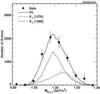
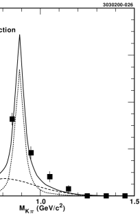
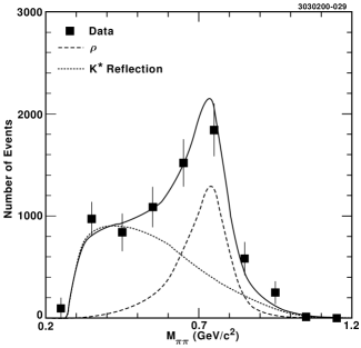
FIG. 2.: Fit to the distributions of $M_{K\pi\pi}$, $M_{K\pi}$ and $M_{\pi\pi}$ with individual components overlaid, after subtracting the non-signal backgrounds in Fig. 1, and after correcting for the relative efficiency as a function of mass. In the upper left plot, the solid line represents the sum of the $\tau\to K_{1}(1270)\nu_{\tau}$ + $\tau\to K_{1}(1400)\nu_{\tau}$ mass spectra and the dashed and dotted lines represent the individual $K_{1}$(1270) and $K_{1}$(1400) contributions. Similarly, the upper right and bottom plots show the $K^{*}\pi$ contributions (dotted) and the $K\rho$ contributions (dashed) to the $K\pi\pi$ final state. The limited statistics of the fitting function is evident in the non-smoothness of the solid curve in these three figures.

TABLE I.: Results for the full fit. In the fit, the parameter $B$ is set to zero and the parameters $C$ and $D$ are constrained by the branching fractions[14] into the $K^{*}\pi$ final state from the $K_{1}(1270)$ and $K_{1}(1400)$, respectively. The parameters $R_{A}$, $R_{B}$, $R_{C}$ and $R_{D}$ are normalizations returned from the fit, as described in the text. Errors for the fit parameters $M$, $\Gamma$ and $f$ are statistical and systematic (respectively), as described in the text.

$A=0.94\pm 0.03\pm 0.04$	$R_{A}=6917$
$B=0.00$ (fixed)	$R_{B}=12403$
$C=0.20$ (constrained)	$R_{C}=61636$
$D=0.27$ (constrained)	$R_{D}=58027$
$\Gamma_{1270}=0.26^{+0.09}_{-0.07}\pm 0.08$ GeV
$\Gamma_{1400}=0.30^{+0.37}_{-0.11}\pm 0.14$ GeV	$f_{1270}=0.66\pm 0.19\pm 0.13$
$M_{1270}=1.254\pm 0.033\pm 0.034$ GeV/$c^{2}$	$f_{\rho}=0.48\pm 0.14\pm 0.10$
$M_{1400}=1.463\pm 0.064\pm 0.068$ GeV/$c^{2}$

The fit results showing contours of constant $\chi^{2}$ in the $M_{1270}$ vs. $M_{1400}$ and $\Gamma_{1270}$ vs. $\Gamma_{1400}$ planes are shown in Figures 3 and 4. (Note that the constraint $M_{1400}>M_{1270}$ is introduced in obtaining Figures 3-4; we therefore fit only over the region above the dashed line.) In these plots, the curves represent 1$\sigma$, 2$\sigma$, 3$\sigma$ and 4$\sigma$ standard deviation error contours around the best fit point (indicated by a cross).

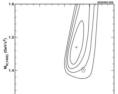
FIG. 3.: Scan of the mass parameter plane showing fit results for the $K_{1}$(1270) mass (horizontal) vs. the $K_{1}$(1400) mass (vertical). Also shown are 1-4 $\sigma$ standard deviation error contours (statistical errors only) around our best fit value (cross) The small open circle shows the present PDG values for the $K_{1}$(1270) and $K_{1}$(1400) masses, with the associated errors (dotted ellipse). The systematic errors for our measurement, although not shown, are nevertheless significant (see text).

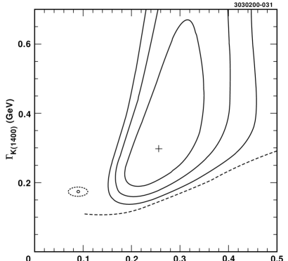
FIG. 4.: Scan of the width parameter plane showing fit results for the $K_{1}$(1270) width (horizontal) vs. the $K_{1}$(1400) width (vertical), as well as contours of constant $\chi^{2}$ (1-3 $\sigma$, statistical errors only). The small open circle shows the present PDG values for the $K_{1}$(1270) and $K_{1}$(1400) widths, with the associated errors (dotted ellipse). The dashed line results from the fitting condition that $M_{K_{1}(1270)}<M_{K_{1}(1400)}$.

We perform a secondary fit, in which the masses and widths of the $K_{1}$ resonances are fixed to world average values [14]. We obtain $f_{1270}=0.40\pm 0.07$, and $f_{\rho}=0.29\pm 0.05$ from this second fit (statistical errors only), to be contrasted with the significantly larger values extracted from our full fit, in which the $K_{1}$ masses and widths are allowed to float as free parameters. It is not surprising that the $f$ values are different in this second fit compared to the original fit, given the high degree of correlation between the $K_{1}$ widths and the relative branching fractions. The $\chi^{2}$ for this second fit is considerably poorer (30.5/22 degrees of freedom) than the primary fit (12.6/18 degrees of freedom).

VIII Systematic uncertainties

Systematic errors are summarized in Table II. The dominant errors are due to the uncertainty in the $K_{1}$ branching fractions and the uncertainty in the background. The errors associated with the uncertainty in the branching fractions of the $K_{1}$ resonances to $K^{*}\pi$ and $K\rho$ are estimated by changing the values for these branching fractions in the form-factors $F_{1}$ and $F_{2}$ by one standard deviation of the PDG values[14]. The resulting spread in the fit values is taken as the corresponding systematic error.

TABLE II.: Summary of systematic error calculations for the full fit. “$K_{1}$ parameters” refers to the uncertainty in the branching fractions, “Model dependence” includes the uncertainty in the kaon momentum spectrum in $\tau^{-}\to K^{-}h^{+}h^{-}\nu_{\tau}$ ($P_{K}$ spectrum). Due to the correlation between momentum and three-prong mass, coupled with the fact that we have good particle identification only over a limited momentum range, uncertainty in $P_{K}$ results in a corresponding uncertainty in the mass spectrum. Other errors are as indicated.

Source		$\Gamma_{1270}$	$\Gamma_{1400}$	$M_{1270}$	$M_{1400}$	$A$	$f_{1270}$	$f_{\rho}$
		GeV	GeV	GeV/$c^{2}$	GeV/$c^{2}$
$K_{1}$ parameters		0.005	0.049	0.005	0.004	0.011	0.016	0.012
Model dependence	$P_{K}$ spectrum	0.057	0.038	0.004	0.020	0.012	0.075	0.055
	$M_{KK\pi}$ shape	0.039	0.107	0.024	0.055	0.010	0.083	0.060
	$\rho^{\prime}$ contribution	0.006	0.001	0.005	0.003	0.012	0.005	0.004
	Vector current	0.015	0.026	0.009	0.005	0.005	0.025	0.025
Background level		0.017	0.054	0.020	0.033	0.028	0.054	0.039
Function and MC statistics		0.019	0.026	0.005	0.006	0.006	0.026	0.019
Total systematic error		0.076	0.140	0.034	0.068	0.037	0.130	0.097

The uncertainty in the background is large because of the uncertainty in the branching fraction of its largest component, $\tau^{-}\to K^{-}K^{+}\pi^{-}\nu_{\tau}$. During the background subtraction the level of all $\tau$-related backgrounds are varied by amounts corresponding to the errors on the branching fractions of these decays [3, 14]. The hadronic background is similarly varied by 100% to determine the systematic error due to our uncertainty in the $q\bar{q}$ background contribution.

Another large error comes from the choice of models in our Monte Carlo simulation. This includes the uncertainty in the shape of the kaon momentum spectrum ($P_{K}$) used to obtain the total number of events with kaons [3], and the uncertainty in the shape of the invariant mass distribution for the $\tau^{-}\to K^{-}K^{+}\pi^{-}\nu_{\tau}$ background. These errors are estimated by using several different models to extract the invariant mass spectra. For $\tau^{-}\to K^{-}\pi^{+}\pi^{-}\nu_{\tau}$, we consider $\tau^{-}\to K_{1}(1270)^{-}\nu_{\tau}$ and $\tau^{-}\to K_{1}(1400)^{-}\nu_{\tau}$ and the model described in [9]; for $\tau^{-}\to K^{-}K^{+}\pi^{-}\nu_{\tau}$, we consider $\tau^{-}\to a^{-}_{1}\nu_{\tau}\to K^{*0}K^{-}\nu_{\tau}$, $\tau^{-}\to\rho(1690)^{-}\nu_{\tau}\to K^{*0}K^{-}\nu_{\tau}$ and the model described in [9].

There are several fitting function uncertainties. The first is the contribution from the $\rho^{\prime}$ which may be different in this decay from that observed in $e^{+}e^{-}\to\pi^{+}\pi^{-}$ data [10] due to the phase space suppression of $\rho^{\prime}$ in our case. Second, the model implemented in our fitting function contains no contribution from the vector current. The corresponding fitting function errors from these two sources are estimated by varying the level of the Wess-Zumino term and the $\rho^{\prime}$ amplitudes from zero to the predictions of [8] and [20]. Another possible source of systematic errors is a phase shift among the interfering decay chains. In this analysis, the parameters $A-D$ in Eqns. (7)-(8) are real. We have done a study of interference effects with additional phase shifts and found that the possible imaginary part of $A-D$ is consistent with zero at our level of sensitivity. Because the fitting function is based upon Monte Carlo, the Monte Carlo statistical error is also included here.

The bias associated with the procedure of fitting the invariant mass distribution is studied using 60 samples of signal Monte Carlo with a full detector simulation. The results of this study show no systematic shift of the fitted parameter values relative to the input values. Additionally, the errors we obtain from analyzing this Monte Carlo sample are fully consistent with statistical expectations.

In this analysis only the shape of the background-subtracted invariant mass distribution is of interest; possible systematic effects that affect the overall normalization of the reconstructed spectra are ignored. Among such effects are trigger and tracking efficiencies, and the photon veto. Non-$\tau$ backgrounds (2-photon events, beam-gas interactions, QED background, e.g.) have been determined to be negligible for the mass spectrum analysis.

IX Discussion of Resonance Structure

A Masses and Widths

As mentioned previously, theoretical predictions for ${\cal B}(\tau\to Kh^{+}h^{-}\nu_{\tau})$ based on ChPT[8] are substantially larger than data. However, if the $K_{1}$ resonances are substantially broader than the PDG values, this discrepancy is resolved. In fact, our data suggest larger $K_{1}$ widths than previous world averages [14] (this is evident from Fig. 2). As indicated in Table I, we extract the masses and widths of the $K_{1}$ resonances from this fit: $\Gamma_{1270}=0.26^{+0.09}_{-0.07}$ GeV, $\Gamma_{1400}=0.30^{+0.37}_{-0.11}$ GeV, $M_{1270}=1.254\pm 0.033$ GeV/$c^{2}$, and $M_{1400}=1.463\pm 0.064$ GeV/$c^{2}$.

In Table III, our result for the widths is compared to the data from ALEPH and DELPHI [15] in their analyses of $\tau$ decays. One observes that all experimental data from $\tau\to K\pi\pi\nu_{\tau}$ for the $K_{1}$ widths are above the current world averages although the errors remain large. The masses of $K_{1}(1270)$ and $K_{1}(1400)$ measured in our analysis are in acceptable agreement with the current world averages [14].

TABLE III.: Current world average and measurements for $\Gamma_{K_{1}}$ from $\tau\to K\pi\pi\nu_{\tau}$.

	$\Gamma_{K_{1}(1270)}$, GeV	$\Gamma_{K_{1}(1400)}$, GeV
PDG [14]	$0.09\pm 0.02$	$0.174\pm 0.013$
ALEPH [15]	$0.37\pm 0.10$	$0.63\pm 0.12$
DELPHI [15]	$0.19\pm 0.07$	$0.31\pm 0.08$
this analysis	$0.26^{+0.09}_{-0.07}\pm 0.08$	$0.30^{+0.37}_{-0.11}\pm 0.14$

B Values of $f_{1270}$ and $f_{\rho}$

As calculated in section VII, our data indicate that there is slightly more $K_{1}(1270)$ than $K_{1}(1400)$ in the axial vector current of the $\tau^{-}\to K^{-}\pi^{+}\pi^{-}\nu_{\tau}$ decay ($f_{1270}=0.66\pm 0.19\pm 0.13$). Other experiments have also investigated the relative contributions of the two $K_{1}$ resonances to $\tau\to s\overline{u}\nu_{\tau}$. One of the first measurements of the $\tau\to K_{1}\nu_{\tau}$ branching fractions was performed by the $TPC/2\gamma$ collaboration in 1994 [16]. Their results are ${\cal B}(\tau\to K_{1}(1270)\nu)=0.41^{+0.41}_{-0.35}$% and ${\cal B}(\tau\to K_{1}(1400)\nu)=0.76^{+0.40}_{-0.33}$%, giving the fraction $f_{1270}=0.35^{+0.73}_{-0.35}$. The results of the $TPC/2\gamma$ experiment suggest that the decay proceeds mostly through $K_{1}(1400)$ although their errors are too large to draw firm conclusions. The latest branching fraction measurements by CLEO [17] and ALEPH [1, 2] as well as this analysis suggest $K_{1}(1270)$ dominance. An analysis of the $K^{-}\pi^{+}$ and $\pi^{-}\pi^{+}$ substructure in $\tau^{-}\to K^{-}\pi^{+}\pi^{-}\nu_{\tau}$ allowed ALEPH[19] to determine $f_{1270}=0.41\pm 0.19\pm 0.15$, based on the known branching fractions of the $K_{1}$ resonances to $K^{*}\pi$ and $K\rho$. Recent measurements therefore favor $K_{1}$(1270) dominance in $\tau^{-}\to K^{-}\pi^{+}\pi^{-}\nu_{\tau}$.

Calculating the amount of $\rho$ in $K\pi\pi$ from the fit parameters we find $f_{\rho}=0.48\pm 0.14$, close to the measurement by ALEPH [19] of $f_{\rho}=0.35\pm 0.11$. This number also agrees with the measurement by ALEPH of another related decay channel, $\tau^{-}\to K^{0}_{S}\pi^{-}\pi^{0}\nu_{\tau}$ where the component $\overline{K}^{0}\rho^{-}$ in the intermediate state is found to be $(64\pm 9\pm 10)\%$, approximately twice that of $K^{-}\rho^{0}$ as expected by isospin symmetries [1].

C $K_{a}-K_{b}$ mixing

From our result for the ratio of $\tau\to K_{1}\nu_{\tau}$ decay amplitudes, information about the mixing of the $K_{a}$ and $K_{b}$ eigenstates can be derived. The mixing between $K_{a}$ and $K_{b}$ is traditionally parameterized in the following way [5]:

$$K_{1}(1400)= K_{a}\cos{\theta_{K}}-K_{b}\sin{\theta_{K}}$$ (17)

$$K_{1}(1270)= K_{a}\sin{\theta_{K}}+K_{b}\cos{\theta_{K}}$$ (18)

In the case of exact $SU(3)_{f}$ symmetry, the second-class current $\tau\to K_{b}\nu_{\tau}$ is forbidden and only $K_{a}$ is produced. However, due to the difference between the masses of the up and strange quarks we may expect symmetry breaking effects of order $|\delta|=(m_{s}-m_{u})/\sqrt{2}(m_{s}+m_{u})\approx 0.18$. Then, instead of pure $K_{a}$ a linear combination $|K_{a}\rangle-\delta|K_{b}\rangle$ is produced and the ratio of decay rates of the $K_{1}$ resonances can be written as [5]:

$$\frac{{\cal B}(\tau\to K_{1}(1270)\nu)}{{\cal B}(\tau\to K_{1}(1400)\nu)}=\left|\frac{\sin{\theta_{K}}-\delta\cos{\theta_{K}}}{\cos{\theta_{K}}+\delta\sin{\theta_{K}}}\right|^{2}\times\Phi^{2}$$ (19)

In this expression, $\Phi$ is the ratio of appropriate kinematical and phase space terms and is calculated by numerical integration. With the parameters measured in this analysis the ratio of branching fractions (Eq. 19) is written as

$$\frac{{\cal B}(\tau\to K_{1}(1270)\nu_{\tau})}{{\cal B}(\tau\to K_{1}(1400)\nu_{\tau})}=\frac{A^{2}R_{A}+C^{2}R_{C}}{D^{2}R_{D}}$$ (20)

From Eqs. (19)-(20), solutions for $\theta_{K}$ can easily be found:

$$\text{(a) }\theta_{K} =(69\pm 16\pm 19)^{\circ}\text{ for $\delta=0.18$},$$ (21)

$$\text{(b) }\theta_{K} =(49\pm 16\pm 19)^{\circ}\text{ for $\delta=-0.18$}.$$ (22)

There is a second pair of solutions that has opposite sign and the same magnitude.

One can also calculate $\theta_{K}$ using the current experimental information on the masses and branching fractions of $K_{1}(1270)$ and $K_{1}(1400)$, independent of their production in $\tau$-decays. There are two possible solutions, $\theta_{K}\approx 33^{\circ}$ and $\theta_{K}\approx 57^{\circ}$ [5]. Our result has the same two-fold ambiguity and is consistent with this calculation.

X Summary and Conclusions

In this analysis we have measured the relative fractions and parameters of the $K_{1}$ resonances in $\tau^{-}\to K^{-}\pi^{+}\pi^{-}\nu_{\tau}$ decays. These measurements are made within the framework of the model described in Sec. VI. Briefly, we assume that $K_{1}$(1270) and $K_{1}$(1400) saturate the $K^{-}\pi^{+}\pi^{-}$ spectrum, and consider only the interference inherent in the Breit-Wigner mass distributions in calculating the relative $\tau^{-}\to K_{1}(1270)\nu_{\tau}$ and $\tau^{-}\to K_{1}(1400)\nu_{\tau}$ branching fractions. Our parameterization of the axial vector form-factors is different from [8] in two respects – our form-factors are motivated by isospin relations, and we assume the Wess-Zumino anomaly to be negligible, as described in Sec. VI. We find $f_{1270}=0.66\pm 0.19\pm 0.13$ and $f_{\rho}=0.48\pm 0.14\pm 0.10$, with $f_{1270}$ and $f_{\rho}$ defined as the $K_{1}(1270)$ and $K\rho$ fractions in $\tau\to K^{-}\pi^{+}\pi^{-}\nu_{\tau}$.

These measurements agree well with the recent results from CLEO and ALEPH (see Sec VII). Our data slightly favor $K_{1}(1270)$ dominance in production of the $K^{-}\pi^{+}\pi^{-}$ final state. The widths that we extract for the $K_{1}$ resonances are considerably larger than previously tabulated values[14]. We also calculate the $K_{a}-K_{b}$ mixing angle, finding $\theta_{K}$ to be consistent with theoretical expectations.

- [1] ALEPH Collaboration, R. Barate et al., Euro. Phys. Jour. C4, 29 (1998).
- [2] ALEPH Collaboration, R. Barate et al., Euro. Phys. Jour. C1, 65 (1998).
- [3] CLEO Collaboration, S. J. Richichi et al., Phys. Rev. D60, 112002 (1999)
- [4] S. Towers, Nuclear Physics B (Proc. Suppl.) C55, 137, 1997; (Proceedings of TAU96: Fourth Workshop on Tau Lepton Physics, Estes Park, Colorado, September 16-19, 1996, ed. J.G. Smith and W. Toki).
- [5] M. Suzuki, Phys. Rev. D47, 1252 (1993).
- [6] A. Weinstein and R. Stroynowski, Ann. Rev. Nucl. Part. Sci. 43, 457 (1993).
- [7] R. Decker, E. Mirkes, R. Sauer, and Z. Was, Z. Phys. C58, 445 (1993).
- [8] M. Finkemeier and E. Mirkes, Z. Phys. C69, 243 (1996).
- [9] S. Jadach, Z.Was, R. Decker and J. H. Kühn, CERN-TH.6793/93.
- [10] J. H. Kühn and A. Santamaria, Z. Phys. C48, 445 (1990).
- [11] CLEO Collaboration, Y. Kubota et al., Nucl. Inst. Meth. 320 66, (1992).
- [12] JETSET 7.3: T. Sjöstrand and M. Bengtsson, Comput. Phys. Commun. 43, 367 (1987).
- [13] R. Brun et al., “GEANT3 Users Guide,” CERN DD/EE/84-1 (1987).
- [14] C. Caso et al., (The Particle Data Group), Eur. Phys. J. C3, 1 (1998)
- [15] J. H. Kühn, E. Mirkes and J. Willibald, hep-ph/9712263 TTP97-53 (presented at International Conference on High Energy Physics, Jerusalem, Israel, 19-26 Aug. 1997).
- [16] D. A. Bauer, Phys. Rev. D50, 10 (1994).
- [17] CLEO Collaboration, T. Coan et al., Phys. Rev. D53, 6037 (1996).
- [18] F. James, CERN Program Library Long Writeup D506 “Function Minimization and Error Analysis Reference Manual”, Version 94.1, CERN, Geneva (1994).
- [19] ALEPH Collaboration, R. Barate et al., Euro. Phys. Jour. C11, 599 (1999).
- [20] B. A. Li, Phys. Rev. D55, 1436 (1997).