Abstract

Two-particle correlations have been measured for identified $\pi^{-}$ from central 158 AGeV Pb+Pb collisions and fitted radii of about 7 fm in all dimensions have been obtained. A multi-dimensional study of the radii as a function of $k_{T}$ is presented, including a full correction for the resolution effects of the apparatus. The cross term $R^{2}_{out-long}$ of the standard fit in the Longitudinally CoMoving System (LCMS) and the $v_{L}$ parameter of the generalised Yano-Koonin fit are compatible with 0, suggesting that the source undergoes a boost invariant expansion.
The shapes of the correlation functions in $Q_{inv}$ and $Q_{space}=\sqrt{Q^{2}_{x}+Q^{2}_{y}+Q^{2}_{z}}$ have been analyzed in detail. They are not Gaussian but better represented by exponentials. As a consequence, fitting Gaussians to these correlation functions may produce different radii depending on the acceptance of the experimental setup used for the measurement.

1 Introduction

The study of Bose-Einstein correlations between pairs of identical hadrons is an essential tool to obtain information on the space-time evolution of the extended hadron sources created in heavy ion collisions [1]. In particular, a strong correlation between the momenta and the space-time production points of the particles suggests expanding sources as predicted by hydrodynamic models [2]. The dynamical evolution of such systems can then be studied with interferometry via selection on the transverse momenta and rapidity of the correlated particle pairs.

In this paper, we present the analysis of two-particle correlations of identified $\pi^{-}$ measured in the WA98 experiment for central 158 AGeV Pb+Pb collisions at the CERN SPS.

2 Experimental setup and data processing

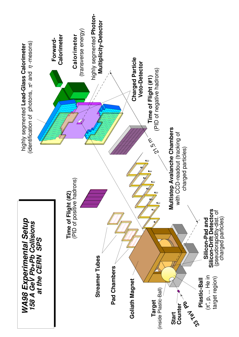
Figure 1: Experimental setup.

The WA98 experiment shown in Fig. 1 combined large acceptance photon detectors with a two arm charged particle tracking spectrometer. The incident 158 AGeV Pb beam interacted with a Pb target near the entrance of a large dipole magnet. Non-interacting beam nuclei, or beam fragments were detected in a forward calorimeter located at zero degree. A mid-rapidity calorimeter measured the total transverse energy in the rapidity region 3.2 $\leq$ $\eta$ $\leq$ 5.4, which was also used in the trigger for online centrality selection. The Plastic-Ball calorimeter measured the fragmentation of the target, and silicon detectors were used to measure the charged particle multiplicity. The photon detectors consisted of a large area photon multiplicity detector and a high granularity lead-glass calorimeter for single photon, $\pi^{0}$, and $\eta$ physics [3].

The charged particle spectrometer made use of a 1.6 Tm dipole magnet with a 2.4$\times$1.6 m² air gap for magnetic deflection of the charged particles in the horizontal plane. The results presented in this paper are taken from the 1995 WA98 data set obtained with the negative particle tracking arm of the charged particle spectrometer. The second tracking arm was added to the spectrometer in 1996 to measure positive particles [4]. The first tracking arm consisted of six multistep avalanche chambers with optical readout [5] located downstream of the magnet. The active area of the first chamber was 1.2$\times$0.8 m², while that of the other five was 1.6$\times$1.2 m². The chambers contained a photoemissive vapour (TEA) which produced UV photons along the path of traversal of the charged particles. These were converted into visible light via wavelength shifter plates. On exit the light was reflected by mirrors at 45^∘ to CCD cameras equipped with two image intensifiers. Each pixel of a CCD viewed a 3.1$\times$3.1 mm² area of a chamber. In addition, a 4$\times$1.9 m² Time of Flight wall positioned behind the chambers at a distance of 16.5 m from the target allowed for particle identification with a time resolution better than 120 ps.

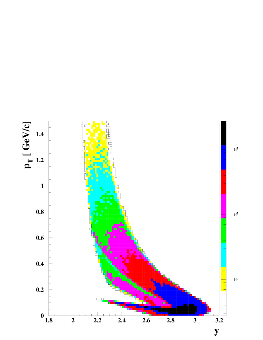
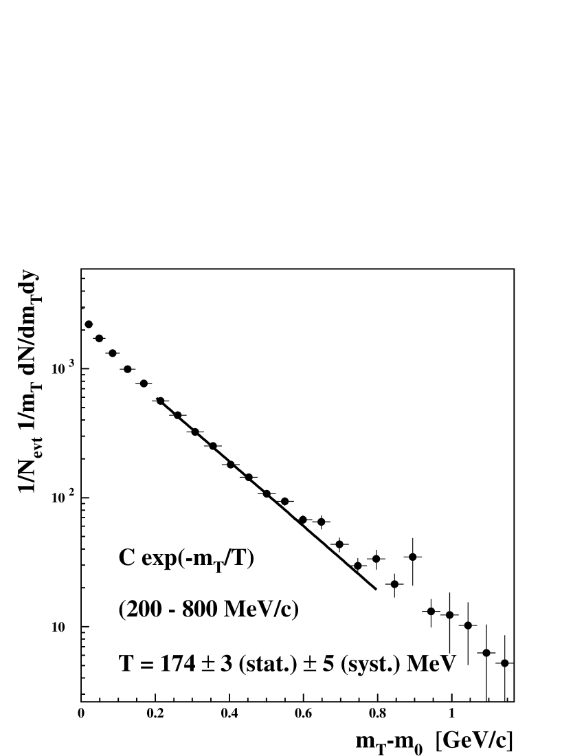
Figure 2: $p_{T}$-rapidity acceptance.

Figure 3: $m_{T}$ distribution (the fit is explained in the text).

Fig. 3 shows the Monte Carlo generated $p_{T}$-rapidity acceptance for $\pi^{-}$. The acceptance ranges from $y$=2.1 to 3.1 with an average at 2.70. The momentum resolution of the spectrometer was $\Delta p/p$=0.005 at $p$=1.5 GeV/c, resulting in an average accuracy better than or equal to 10 MeV/c for all the Q variables used in the interferometry analysis and defined in section 5: ${\sigma}(Q_{inv})$=7 MeV/c, ${\sigma}(Q_{TO})$=10 MeV/c, ${\sigma}(Q_{TS})$=5 MeV/c, ${\sigma}(Q_{L})$=3 MeV/c, ${\sigma}(Q_{T})$=8 MeV/c, ${\sigma}(Q_{0})$=5 MeV/c.

The analysis of the complete 1995 data set is presented here. These data have been taken with the most central triggers corresponding to about 10% of the minimum bias cross section of 6190 mb. Severe track quality cuts were applied at the expense of statistics resulting in final samples of 4.2$\times 10^{6}$ $\pi^{-}$ for the correlation analysis and 4.6$\times 10^{5}$ $\pi^{-}$ for the single particle spectrum.

3 Single particle spectra

The $m_{T}$=$\sqrt{m_{\pi}^{2}+p_{T}^{2}}$ distribution of identified $\pi^{-}$, averaged over the rapidity acceptance, is shown in Fig. 3. The data were corrected for geometrical acceptance and efficiency of the chamber-camera-Time of Flight system using a full simulation of the experimental setup. The parameters of the simulation were optimized in an iterative way by comparing various distributions with the real data. The simulated data were then treated exactly like the real data. The measured $1/m_{T}\,dN/dm_{T}\>dy$ distribution was then fitted to the form $C$exp$(-m_{T}/T)$, expected for a source in thermal equilibrium [6]. Such fits were applied to the data for different ranges of $m_{T}$, such as the one shown in Fig. 3. These fits do not reproduce the overall concave shape of the data, which is partly due to particles originating in resonance decays and could also be an indication of transverse flow [7]. The shape of the $\pi^{-}$ $m_{T}$ distribution was found to be in good agreement with that of $\pi^{0}$ obtained in the lead-glass calorimeter [3].

4 One-dimensional interferometry analysis

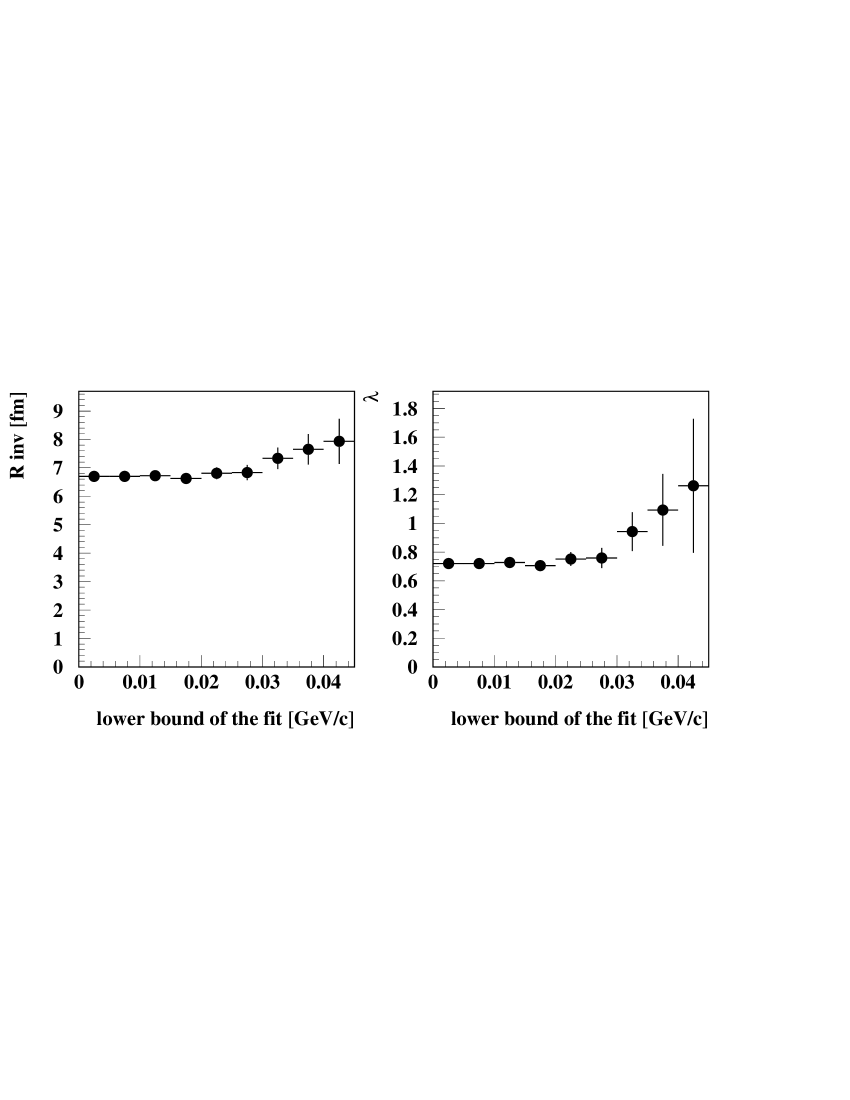
Figure 6: Gaussian fit stability.

Figure 7: Exponential fit stability.

For the Bose-Einstein correlation studies, the data were Coulomb corrected in an iterative way [8]. The Gamow correction was abandoned as it overcorrects the data for $Q_{inv}$ in the range of 0.1 to 0.3 GeV/c. A fit of the form $1+\lambda\mbox{exp}[-Q^{2}_{inv}R^{2}_{inv}]$ was made to the $Q_{inv}$ correlation function yielding $R_{inv}=6.83\pm 0.10$ fm and $\lambda=0.307\pm 0.008$. An expanded view of the correlation distribution (Fig. 5) shows that the Gaussian fit used (full line) is not perfect, especially in the $Q_{inv}$ range of 40 to 80 MeV/c where the tail of the experimental distribution shows an excess which is not well reproduced by the fit. In addition to this Gaussian fit made over the whole range of $Q_{inv}$, Fig. 5 shows also different Gaussian fits using data in the ranges 25 MeV/c $\leq$ $Q_{inv}$ $\leq$ 200 MeV/c (dashed line) and 40 MeV/c $\leq$ $Q_{inv}$ $\leq$ 200 MeV/c (dotted line). These fits do not coincide. Different radii are then obtained for different starting points of the fit because the shape of the distribution is not Gaussian. This effect is independent of the severity of the track selection, and is therefore not due to spurious tracks. This is summarized in Fig. 7 where $R_{inv}$ and the corresponding $\lambda$ are plotted as a function of the lower bound of the fit. There is a statistically significant drop when using a Gaussian fit. A similar behaviour is observed when, instead of $Q_{inv}$, $Q_{space}=\sqrt{Q^{2}_{x}+Q^{2}_{y}+Q^{2}_{z}}$ is used, calculated in the longitudinally comoving system (LCMS) and fitted with 1+$\lambda$exp[-$Q^{2}_{3}R^{2}_{3}]$. This method of fitting in varying ranges has a good sensitivity to the shape. It has been repeated by replacing the Gaussian fit by an exponential fit of the form 1+$\lambda_{e}$exp[-2$Q_{inv}R_{e}]$ where the factor 2 is added to make the radius $R_{e}$ more comparable with $R_{inv}$. The results (Fig. 7) show that the stability is better with the exponential fit. Fig. 5 directly compares the Gaussian and exponential fits for $Q_{inv}$. Although the Gaussian fit still gives an acceptable $\chi^{2}/$d.o.f., the exponential fit is better everywhere. A similar conclusion is reached when the first data point is excluded from the fit. This result is not based on the first bins which might be more affected by systematics due to large Coulomb correction or noise correlated with the true track signals in the chambers. It is rather based on the high statistics tail of the distribution which contributes in a different way to a Gaussian or an exponential fit. This quasi exponential behaviour is expected by different models including resonance decays [9]. As a consequence small acceptance experiments may obtain a larger radius if a Gaussian fit is used because they are less sensitive to the tail. On the contrary large acceptance experiments have higher statistics at large $Q$-values, and the Gaussian fit will yield lower values of the radius.

5 Multi-dimensional interferometry analysis

The multi-dimensional analysis has been done with Gaussian fits to allow comparison with other experiments. Two different parameterizations have been used in the LCMS:

a) The standard fit in the 3-dimensional space of momentum differences $Q_{TS}$ (perpendicular to the beam axis and to the transverse momentum of the pair), $Q_{TO}$ (perpendicular to the beam axis and parallel to the transverse momentum of the pair), and $Q_{L}$ (parallel to the beam axis) [10]. The fitted formula

$$C_{2}=1+\lambda\exp[-Q_{TS}^{2}R_{TS}^{2}-Q_{TO}^{2}R_{TO}^{2}-Q_{L}^{2}R_{L}^{2}-2Q_{TO}Q_{L}R^{2}_{out-long}]$$

includes a cross term in $Q_{TO}Q_{L}$ as predicted [11].

b) The generalized Yano-Koonin (GYK) fit [12] in the $Q_{0}$ (energy difference of the pair), $Q_{T}$,$Q_{L}$ space according to

$$C_{2}=1+\lambda\exp[-Q^{2}_{T}R^{2}_{T}+(Q^{2}_{0}-Q^{2}_{L})R^{2}_{4}-(Q{\cdot}U)^{2}(R^{2}_{0}+R^{2}_{4})]$$

where $U=\gamma(1,0,0,v_{L})$, $\gamma=1/\sqrt{1-v_{L}^{2}}$ with $v_{L}$ in units of c=1.

In the GYK approach, the radius parameters remain invariant under longitudinal Lorentz boost, the parameter $v_{L}$ connecting the “arbitrary” measurement frame (LCMS) to the Yano-Koonin frame. In addition, the extraction of the duration of emission, $R_{0}$, is straightforward.

The consequence of the finite resolution in the measurement of the $Q$ variables is an underestimate of the radii and $\lambda$ parameters. Morever, as the resolution is different for each $Q$ variable, this causes a bias which varies from parameter to parameter, leading to errors in the interpretation of the results in a multi-dimensional analysis. It is therefore essential to take into account the effect of the resolution in the fitting procedure. One way to do this is to replace the formula $C_{2}(\vec{Q})$ used to fit the data by

$$C_{2}^{rc}(\vec{Q})=\int\!\!\int\!\!\int r(\vec{Q},\vec{Q^{\prime}})\>C_{2}(\vec{Q^{\prime}})\>d\vec{Q^{\prime}}$$

which is the convolution of $C_{2}(\vec{Q})$ with the resolution function $r(\vec{Q},\vec{Q^{\prime}})$. The resolution function is chosen to be Gaussian:

$$r(\vec{Q},\vec{Q^{\prime}})=1/(2\pi)^{3/2}\>1/|V|^{1/2}\>\exp[-1/2\>(\vec{Q}-\vec{Q^{\prime}})^{T}\>V^{-1}\>(\vec{Q}-\vec{Q^{\prime}})]$$

The diagonal elements of the covariance matrix $V$ are equal to the square of the resolution of the different $Q$ variables and are estimated separately as a function of $k_{T}=|\vec{p}_{T1}+\vec{p}_{T2}|/2$ of the pairs. The non-diagonal elements are neglected. For the one-dimensional Gaussian fit case with $\vec{Q}=Q_{inv}$, the resolution corrected values of the fitted parameters are $R_{inv}=7.30\pm 0.12$ fm and $\lambda=0.328\pm 0.009$.

Table 1: 3-dimensional analysis

Standard fit in LCMS				Generalized Yano-Koonin fit
$R_{TS}$	=	6.41$\pm$	0.13 fm	$R_{T}$	=	6.54$\pm$	0.11 fm
$R_{TO}$	=	6.60$\pm$	0.16 fm	$R_{0}$	=	0.01$\pm$	0.69 fm
$R_{L}$	=	7.50$\pm$	0.18 fm	$R_{4}$	=	7.51$\pm$	0.18 fm
$\lambda$	=	0.350$\pm$	0.010	$\lambda$	=	0.325$\pm$	0.009
$R^{2}_{out-long}$	=	-1.0$\pm$	1.3 fm2	$v_{L}$	=	0.03$\pm$	0.05
$\chi^{2}/$d.o.f.	=	1.06		$\chi^{2}/$d.o.f.	=	1.02

The results of the multi-dimensional fits are presented in Table 1 for the full 1995 data sample. A multi-dimensional analysis as a function of $k_{T}$, both with the standard 5-parameter fit and with the GYK fit is shown in Figs. 8, 9, and 10.

The $R_{TS}$ and $R_{L}$ parameters from the standard fit are found to be compatible respectively with $R_{T}$ and $R_{4}$ from the GYK fit. The cross term $R^{2}_{out-long}$ from the standard fit and $v_{L}$ from the GYK fit are compatible with 0. In a source undergoing a boost invariant expansion, the local rest frame coincides with the LCMS. Both the cross term and $v_{L}$ estimated in the LCMS are then expected to vanish [12]. As this is the case, it suggests that the source seen within the acceptance of the experiment has a strictly boost invariant expansion. The strong decrease of the longitudinal radius $R_{L}$ or $R_{4}$ with $k_{T}$ compared to the behaviour of the transverse radii $R_{T}$, $R_{TS}$, $R_{TO}$ suggests a longitudinal expansion larger than the lateral expansion. The longitudinal radius $R_{L}$ is shown with a fit of the form 1/$\sqrt{m_{T}}$ with ${m_{T}}$=$\sqrt{m_{\pi}^{2}+k_{T}^{2}}$ inspired by the hydrodynamical expansion model. Using $R_{L}=\tau_{0}\sqrt{T_{0}/m_{T}}$ with a freeze out temperature $T_{0}$ of 120-170 MeV/c, we may extract a freeze out time $\tau_{0}$ in the range of 7.5-8.9 fm/c. Finally, the $R_{0}$ parameter from the GYK fit, which reflects the duration of emission, is compatible with 0 for all $k_{T}$ bins, excluding a long-lived intermediate phase.

Two other experiments, NA49 and NA44, have studied charged particle interferometry in Pb+Pb collisions at CERN energies. The WA98 analysis is in good agreement with the NA49 results[13], when the comparison is made for the same mean $y$ range of 2.70, although WA98 has used identified $\pi^{-}$ while the NA49 analysis used unidentified negative particles. Only the $R_{0}$ parameter tends to be smaller in WA98. The direct comparison with the NA44 experiment is not possible because NA44 and WA98 do not have the same $y$ range. The smaller radii measured by NA44[14] can be explained by the larger $y$ range of its acceptance (3.1$<y<$4.1).

6 Conclusion

The analysis of the two-particle correlation of identified $\pi^{-}$ from central Pb+Pb collisions at 158 AGeV gives fitted radii of about 7 fm. This should be compared to the equivalent rms radius of the initial Pb nucleus of 3.2 fm, which indicates a large final state emission volume.

The one-dimensional correlation functions analyzed in terms of $Q_{inv}$ or $Q_{space}$ are not Gaussian. They are better represented by exponentials. This study is based on the tail of the distributions and not on the first bins which might be subject to systematic effects. One possible explanation is that this behaviour is due to resonance effects. Fitting Gaussians to these correlation functions may produce different results depending on the acceptance of the experimental setup.

The generalized Yano-Koonin analysis gives similar results to within the error bars as the standard 3-dimensional analysis in the LCMS.

The cross term $R^{2}_{out-long}$ is found to be compatible with 0 in the LCMS and the same is true of $v_{L}$ in the GYK fit. This suggests that the source undergoes a boost invariant expansion.

A clear dependence of the longitudinal radius parameter on $k_{T}$ is observed, suggesting a larger longitudinal than transverse expansion of the source. In addition the short duration of emission disfavours any long-lived intermediate phase.

Acknowledgements
    We would like to thank the CERN-SPS accelerator crew for providing an excellent lead beam and the Laboratoire National Saturne for the loan of the magnet Goliath.

This work was supported jointly by the German BMBF and DFG, the U.S. DOE, the Swedish NFR, the Dutch Stichting FOM, the Swiss National Fund, the Humboldt Foundation, the Stiftung für deutsch-polnische Zusammenarbeit, the Department of Atomic Energy, the Department of Science and Technology and the University Grants Commission of the Government of India, the Indo-FRG Exchange Programme, the PPE division of CERN, the INTAS under contract INTAS-97-0158, the Polish KBN under the grant 2P03B16815, and ORISE. ORNL is managed by Lockheed Martin Energy Research Corporation under contract DE-AC05-96OR22464 with the U.S. Department of Energy.

Figure 4: $Q_{inv}$ distribution with Gaussian fits. The full line is a fit made with all the points. The dashed line is a fit for $Q_{inv}\geq 25$ MeV/c and the dotted line is a fit for $Q_{inv}\geq 40$ MeV/c.

Figure 5: $Q_{inv}$ distribution with the Gaussian fit (full line) and the exponential fit (dashed line).

Figure 8: 5-parameter fit as a function of $k_{T}$. The horizontal bars indicate the bin width and the points are plotted at the average $k_{T}$ of the bin. The dashed line in the bottom left figure shows the result of a fit explained in the text.

Figure 9: Comparison of the $R_{TS}$ and $R_{L}$ parameters from the standard fit respectively with $R_{T}$ and $R_{4}$ from the GYK fit as a function of $k_{T}$.

Figure 10: The cross term $R^{2}_{out-long}$ from the standard fit and $v_{L}$ from the GYK fit, both estimated in the LCMS, are compatible with 0 for all $k_{T}$ bins.

References

- [1] W. Zajc et al., Phys. Rev. C29 (1984) 2173 and references therein.
-
[2]
T. Csörgő et al., Phys. Lett. B347
(1995) 354.
T. Csörgő et al., Phys. Lett. B338 (1994) 134. -
[3]
T. Peitzmann et al., Nucl. Phys. A610 (1996) 200c.
M.M. Aggarwal et al., Phys. Rev. Lett. 81 (1998) 4087. -
[4]
L. Carlen et al., Nucl. Instr. and Meth. A412
(1998) 361.
L. Carlen et al., Nucl. Instr. and Meth. A413 (1998) 92. -
[5]
J.M. Rubio et al., Nucl. Instr. and Meth. A367
(1995) 358.
A.L.S. Angelis et al., Nucl. Phys. A566 (1994) 605c.
M. Iżycki et al., Nucl. Instr. and Meth. A310 (1991) 98. - [6] E. Schnedermann et al., Phys. Rev. C48 (1993) 2462.
- [7] M.M. Aggarwal et al., Phys. Rev. Lett. 83 (1998) 926.
- [8] S.Pratt et al., Phys. Rev. C42 (1990) 2646; these calculations were made with a Fortran program supplied by S. Pratt.
-
[9]
S. Padula and M. Gyulassy, Nucl. Phys. A525
(1991) 339.
U.A. Wiedemann et al., Phys. Rev. C53 (1996) 918. -
[10]
S. Pratt, Phys. Rev. D33 (1986) 1314.
G. Bertsch and G.E. Brown, Phys. Rev. C40 (1989) 1830. - [11] S. Chapman et al., Phys. Rev. Lett. 74 (1995) 4400.
- [12] S. Chapman et al., Phys. Rev. C52 (1995) 2694 and references therein.
- [13] H. Appelshäuser et al., Eur. Phys. J. C2 (1998) 661.
- [14] I.G. Bearden et al., Phys. Rev. C58 (1998) 1656.