Enhancing the physical significance of Frequentist confidence intervals

Abstract

It is shown that all the Frequentist methods are equivalent from a statistical point of view, but the physical significance of the confidence intervals depends on the method. The Bayesian Ordering method is presented and confronted with the Unified Approach in the case of a Poisson process with background. Some criticisms to both methods are answered. It is also argued that a general Frequentist method is not needed.

1 Introduction

In this report I will be concerned mainly with the Frequentist (classical) theory of statistical inference, but I think that it is interesting and useful that I express my opinion on the war between Frequentists and Bayesians. To the question

“Are you Frequentist or Bayesian”?

I answer

“I like statistics.”

I think that if one likes statistics, one can appreciate the beauty of both Frequentist and Bayesian theories and the subtleties involved in their formulation and application. I think that both approaches are valid from a statistical as well as physical point of view. Their difference arises from different definitions of probability and their results answer different statistical questions. One can like more one of the two theories, but I think that it is unreasonable to claim that only one of them is correct, as some partisans of that theory claim. These partisans often produce examples in which the other approach is shown to yield misleading or paradoxical results. I think that each theory should be appreciated and used in its limited range of validity, in order to answer the appropriate questions. Finding some example in which one approach fails does not disprove its correctness in many other cases that lie in its range of validity.

My impression is that the Bayesian theory (see, for example, [1]) has a wider range of validity because it can be applied to cases in which the experiment can be done only once or a few times (for example, our thoughts in everyday decisions and judgments seem to follow an approximate Bayesian method). In these cases the Bayesian definition of probability as degree of believe seems to me the only one that makes sense and is able to provide meaningful results.

Let me remind that since Galileo an accepted basis of scientific research is the repeatability of experiments. This assumption justifies the Frequentist definition of probability as ratio of the number of positive cases and total number of trials in a large ensemble. The concept of coverage follows immediately: a $100\alpha\%$ confidence interval for a physical quantity $\mu$ is an interval that contains (covers) the unknown true value of that quantity with a Frequentist probability $\alpha$. In other words, a $100\alpha\%$ confidence interval for $\mu$ belongs to a set of confidence intervals that can be obtained with a large ensemble of experiments, $100\alpha\%$ of which contain the true value of $\mu$.

2 The statistical and physical significance of confidence intervals

I think that in order to fully appreciate the meaning and usefulness of Frequentist confidence intervals obtained with Neyman’s method [2, 3], it is important to understand that the experiments in the ensemble do not need to be identical, as often stated, or even similar, but can be real, different experiments [2, 4]. One can understand this property in a simple way [5] by considering, for example, two different experiments that measure the same physical quantity $\mu$. The $100\alpha\%$ classical confidence interval obtained from the results of each experiment belongs by construction to a set of confidence intervals which can be obtained with an ensemble of identical experiments and contain the true value of $\mu$ with probability $\alpha$. It is clear that the sum of these two sets of confidence intervals, containing the two confidence intervals obtained in the two different experiments, is still a set of confidence intervals that contain the true value of $\mu$ with probability $\alpha$.

Moreover, for the same reasons it is clear that the results of different experiments can also be analyzed with different Frequentist methods [6], i.e. methods with correct coverage but different prescriptions for the construction of the confidence belt. This for me is amazing and beautiful: whatever method you choose you get a result that can be compared meaningfully with the results obtained by different experiments using different methods! It is important to realize, however, that the choice of the Frequentist method must be done independently of the knowledge of the data (before looking at the data), otherwise the property of coverage is lost, as in the “flip-flop” example in Ref. [7].

This property allow us to solve an apparent paradox that follows from the recent proliferation of proposed Frequentist methods [7, 8, 9, 10, 11, 12]. This proliferation seems to introduce a large degree of subjectivity in the Frequentist approach, supposed to be objective, due to the need to choose one specific prescription for the construction of the confidence belt, among several available with similar properties. From the property above, we see that whatever Frequentist method one chooses, if implemented correctly, the resulting confidence interval can be compared statistically with the confidence intervals of other experiments obtained with other Frequentist methods. Therefore, the subjective choice of a specific Frequentist method does not have any effect from a statistical point of view!

Then you should ask me:

Why are you proposing a specific Frequentist method?

The answer lies in physics, not statistics. It is well known that the statistical analysis of the same data with different Frequentist methods produce different confidence intervals. This difference is sometimes crucial for the physical interpretation of the result of the experiment (see, for example, [8, 10]). Hence, the physical significance of the confidence intervals obtained with different Frequentist methods is sometimes crucially different. In other words, the Frequentist method suffers from a degree of subjectivity from a physical, not statistical, point of view.

3 The beauty of the Unified Approach and its pitfalls

The possibility to apply successfully Frequentist statistics to problematic cases in frontier research has received a fundamental contribution with the proposal of the Unified Approach by Feldman and Cousins [7]. The Unified Approach consists in a clever prescription for the construction of “a classical confidence belt which unifies the treatment of upper confidence limits for null results and two-sided confidence intervals for non-null results”.

In the following I will consider the case of a Poisson process with signal $\mu$ and known background $b$. The probability to observe $n$ events is

$$P(n|\mu,b)=\frac{(\mu+b)^{n}e^{-(\mu+b)}}{n!}\,.$$ (1)

The Unified Approach is based on the construction of the acceptance intervals $[n_{1}(\mu),n_{2}(\mu)]$ ordering the $n$’s through their rank given by the relative magnitude of the likelihood ratio

$$R(n,\mu,b)=\frac{P(n|\mu,b)}{P(n|\mu_{\mathrm{best}},b)}=\left(\frac{\mu+b}{\mu_{\mathrm{best}}+b}\right)^{n}e^{\mu_{\mathrm{best}}-\mu}\,,$$ (2)

where $\mu_{\mathrm{best}}$ is the maximum likelihood estimate of $\mu$,

$$\mu_{\mathrm{best}}(n,b)=\mathrm{Max}[0,n-b]\,.$$ (3)

As a result of this construction the confidence intervals are two-sided (i.e. $[\mu_{\mathrm{low}},\mu_{\mathrm{up}}]$ with $\mu_{\mathrm{low}}>0$) for $n\gtrsim b$, whereas for $n\lesssim b$ they are upper limits (i.e. $\mu_{\mathrm{low}}=0$).

The fact that the confidence intervals are two-sided for $n\gtrsim b$ can be understood by considering $n>b$, that gives $\mu_{\mathrm{best}}=n-b$. In this case the likelihood ratio (2) is given by

$$R(n>b,\mu,b)=\left(\frac{\mu+b}{n}\right)^{n}e^{n-(\mu+b)}=\exp\left\{n\left[1+\ln(\mu+b)-\ln{n}\right]-(\mu+b)\right\}\stackrel{{\scriptstyle n\to\infty}}{{\longrightarrow}}0\,.$$ (4)

This implies that the rank of high values of $n$ is very low and they are excluded form the confidence belt. Therefore, the acceptance intervals $[n_{1}(\mu),n_{2}(\mu)]$ are always bounded, i.e. $n_{2}(\mu)$ is finite, and the confidence intervals are two-sided for $n\gtrsim b$, as illustrated in Fig. 2, where the solid lines show the borders of the confidence belt for a background $b=5$ and a confidence level $\alpha=0.90$.

Figure 1: Confidence belt in the Unified Approach for background $b=5$ and confidence level $\alpha=0.90$.

Figure 2: Confidence belt in the Unified Approach for background $b=5$ and confidence level $\alpha=0.50$.

The fact that the confidence intervals are upper limits for $n\lesssim b$ can be understood by considering $n\leq b$, for which we have $\mu_{\mathrm{best}}=0$ and the likelihood ratio that determines the ordering of the $n$’s in the acceptance intervals is given by

$$R(n{\leq}b,\mu,b)=\left(1+\frac{\mu}{b}\right)^{n}\,e^{-\mu}\,.$$ (5)

Considering now the acceptance interval for $\mu=0$, we have $R(n\leq b,\mu=0,b)=1$. Therefore, all $n\leq b$ for $\mu=0$ have highest rank and are guaranteed to lie in the confidence belt. This is illustrated in Fig. 2, where the thick solid segment shows the $n\leq b$ part of the acceptance interval for $\mu=0$, that must lie in the confidence belt. Since $\mu$ is a continuous parameter, also for small values of $\mu$ the $n\leq b$ have rank close to the highest one and lie in the confidence belt. Indeed, for $\mu>0$, the likelihood ratio (2) increases for $n$ going form zero to the largest integer smaller or equal to $b$ and decreases for larger values of $n$. Hence, the largest integer $n_{\mathrm{hr}}$ such that $n_{\mathrm{hr}}\leq b$ has highest rank. If $\mu$ is sufficiently small all $n\leq b$ have rank close to maximum and are included in the confidence belt if the confidence level is large enough, $\alpha\gtrsim 0.60$. For example, $R(n=0,\mu,b)>R(n_{\mathrm{hr}}+1,\mu,b)$ for $\mu<(1+b)e^{-1/(1+b)}-b$. Therefore, the left edge of the confidence belt must change its slope for $n\lesssim b$ and intercept the $\mu$-axis at a positive value of $\mu$, as illustrated in Fig. 2. The value of $\mu$ at which the left edge of the confidence belt intercepts the $\mu$-axis, that corresponds to $\mu_{\mathrm{up}}(n=0)$, depends on the value of the background $b$ and on the value of the confidence level $\alpha$.

However, for small values of $\alpha$ the Unified Approach gives zero-width confidence intervals for $n\ll b$, as illustrated in Fig. 2, where I have chosen $b=5$ and $\alpha=0.50$. One can see that the segment $n\leq b$ is enclosed in the confidence belt for $\mu=0$, but for any value of $\mu>0$ the sum of the probabilities of the $n$’s close to $\mu+b$ is enough to reach the confidence level and low values of $n$ are not included in the confidence belt. Hence, in this case the Unified Approach gives zero-width confidence intervals for $n<2$.

The unification of the treatments of upper confidence limits for null results and two-sided confidence intervals for non-null results obtained with the Unified Approach is wonderful, but it has been noticed that the upper limits obtained with the Unified Approach for $n<b$ are too stringent (meaningless) from a physical point of view [8, 13]. In other words, although these limits are statistically correct from a Frequentist point of view, they cannot be taken as reliable upper bounds to be used in physical applications.

This problem is illustrated in Fig. 3A, where I plotted the 90% CL upper limit $\mu_{\mathrm{up}}$ as a function of $b$ for $n=0,\ldots,5$. The solid part of each line shows where $b\geq n$. One can see that for a given $n$, $\mu_{\mathrm{up}}$ decreases rather steeply when $b$ is increased, until a minimum value close to one is reached. The curves have jumps because $n$ is an integer and generally the desired confidence level cannot be obtained exactly, but with some unavoidable overcoverage.

Figure 3: 90% CL upper limit $\mu_{\mathrm{up}}$ as a function of the background $b$ for $n=0$ (lower lines), $\ldots$, $n=5$ (upper lines). The solid part of each line shows where $b\geq n$.

Let me emphasize that the problem of obtaining too stringent upper limits for $n<b$ is very serious for a scientist that wants to obtain reliable information from experiment and use this information for other purposes (as input for a theory or another experiment). In the past, researchers bearing the same physical point of view refrained to report empty confidence intervals or very stringent upper limits when $n<b$ was measured. These confidence intervals are correct from a statistical point of view, but useless from a physical point of view. Furthermore, the same reasoning lead to prefer the Unified Approach to central confidence intervals or upper limits, because the non-empty confidence interval obtained when $n<b$ is measured is certainly more significant, from a physical point of view, than an empty one, although they are statistically equivalent, as shown in Section 2.

4 A brutal modification of the Unified Approach

In the Unified Approach $\mu_{\mathrm{best}}$ is positive and equal to zero for $n\leq b$. If $\mu_{\mathrm{best}}$ is forced to be always bigger than zero, the $n$’s smaller than $b$ have rank higher than in the Unified Approach. As a consequence, the decrease of the upper limit $\mu_{\mathrm{up}}$ as $b$ increases is weakened. This is illustrated by a “Brutally Modified Unified Approach” (BMUA) in which we take

$$\mu_{\mathrm{best}}=\mathrm{Max}[\mu_{\mathrm{best}}^{\mathrm{min}},n-b]\,,$$ (6)

where $\mu_{\mathrm{best}}^{\mathrm{min}}$ is a positive real number.

In Fig. 5 I plotted the confidence belts for $\mu_{\mathrm{best}}^{\mathrm{min}}=0$ (solid lines), that corresponds to the Unified Approach, $\mu_{\mathrm{best}}^{\mathrm{min}}=1$ (dashed lines) and $\mu_{\mathrm{best}}^{\mathrm{min}}=2$ (dotted lines), for $b=10$. One can see that in the BMUA the upper limits of the confidence intervals are considerably higher than in the Unified Approach. The behavior of $\mu_{\mathrm{up}}$ as a function of $b$ for $n=0$ is shown in Fig. 5, from which it is clear that the decrease of $\mu_{\mathrm{up}}$ when $b$ increases is much weaker in the BMUA (dashed and dotted lines) than in the Unified Approach (solid line) and it is almost absent for $\mu_{\mathrm{best}}^{\mathrm{min}}\gtrsim 2$.

Figure 4: 90% confidence belts for $b=10$ in the Unified Approach ($\mu_{\mathrm{best}}^{\mathrm{min}}=0$, solid lines) and in the Brutally Modified Unified Approach (BMUA) for $\mu_{\mathrm{best}}^{\mathrm{min}}=1$ (dashed lines) and $\mu_{\mathrm{best}}^{\mathrm{min}}=2$ (dotted lines).

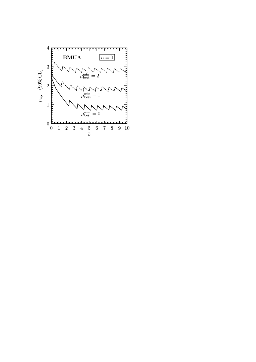
Figure 5: 90% CL upper limit $\mu_{\mathrm{up}}$ as a function of the background $b$ for $n=0$ in the Unified Approach ($\mu_{\mathrm{best}}^{\mathrm{min}}=0$, solid line) and in the BMUA for $\mu_{\mathrm{best}}^{\mathrm{min}}=1$ (dashed line) and $\mu_{\mathrm{best}}^{\mathrm{min}}=2$ (dotted line).

Let me emphasize that

1. The BMUA is a statistically correct Frequentist method and coverage is satisfied.

2. In the BMUA one obtains upper limits for $n\lesssim b$ and central confidence intervals for $n\gtrsim b$, as in the Unified Approach.

3. The BMUA method is not general (although it can be extended in an obvious way at least to the case of a gaussian variable with a physical boundary).

4. I am not proposing the BMUA! (But those that think that the upper limit for $n=0$ should not depend on $b$ may consider the possibility of using the BMUA with $\mu_{\mathrm{best}}^{\mathrm{min}}=2$ instead of resorting to more complicated methods that may even jeopardize the property of coverage.)

As shown in Fig. 5, the right edge of the confidence belt in the BMUA is not very different from the one in the Unified Approach. This is due to the fact that adding small values of $n$ with low probability to the acceptance intervals has little effect. Moreover, it is clear that the acceptance interval for $\mu=0$ is equal for all Frequentist methods with correct coverage that unify the treatment of upper confidence limits and two-sided confidence intervals.

5 Bayesian Ordering

An elegant, natural and general way to obtain automatically $\mu_{\mathrm{best}}^{\mathrm{min}}>0$ is given by the Bayesian Ordering method [8], in which $\mu_{\mathrm{best}}$ is replaced by the Bayesian expectation value for $\mu$, $\mu_{\mathrm{B}}$.

Choosing a natural flat prior, the Bayesian expectation value for $\mu$ in a Poisson process with background is given by

$$\mu_{\mathrm{B}}(n,b)=n+1-\left(\sum_{k=0}^{n}\frac{kb^{k}}{k!}\right)\left(\sum_{k=0}^{n}\frac{b^{k}}{k!}\right)^{-1}=n+1-b\left(\sum_{k=0}^{n-1}\frac{b^{k}}{k!}\right)\left(\sum_{k=0}^{n}\frac{b^{k}}{k!}\right)^{-1}\,.$$ (8)

The obvious inequality $\sum_{k=0}^{n}k\,b^{k}/k!\leq n\sum_{k=0}^{n}b^{k}/k!$ implies that $\mu_{\mathrm{B}}\geq 1$. Therefore, the reference value for $\mu$ in the likelihood ratio

$$R(n,\mu,b)=\frac{P(n|\mu,b)}{P(n|\mu_{\mathrm{B}},b)}=\left(\frac{\mu+b}{\mu_{\mathrm{B}}+b}\right)^{n}e^{\mu_{\mathrm{B}}-\mu}\,,$$ (9)

that determines the construction of the acceptance intervals as in the Unified Approach, is bigger or equal than one. As a consequence, the decrease of the upper confidence limit $\mu_{\mathrm{up}}$ for a given $n$ when the expected background $b$ increases is significantly weaker than in the Unified Approach, as illustrated in Fig. 3B.

Figure 3C shows $\mu_{\mathrm{up}}$ as a function of $b$ in the Bayesian Theory with a flat prior and shortest credibility intervals. One can see that the behavior of $\mu_{\mathrm{up}}$ obtained with the Bayesian Ordering method is intermediate between those in the Unified Approach and in the Bayesian Theory. Although one must always remember that the statistical meaning of $\mu_{\mathrm{up}}$ is different in the two Frequentist methods (Unified Approach and Bayesian Ordering) and in the Bayesian Theory, for scientists using these upper limits it is often irrelevant how they have been obtained. Hence, I think that an approximate agreement between Frequentist and Bayesian results is desirable.

Figure 6: Confidence belt obtained with the Bayesian Ordering for background $b=5$ and confidence level $\alpha=0.90$.

Figure 7: Confidence belt obtained with the Bayesian Ordering for background $b=5$ and confidence level $\alpha=0.50$.

From Eq. (8) one can see that

$$n\gg b \quad\Longrightarrow\quad \mu_{\mathrm{B}}(n,b)\simeq n+1-b\simeq n\,,$$ (12)

$$n\lesssim b\,,\quad b\gg 1 \quad\Longrightarrow\quad \mu_{\mathrm{B}}(n,b)\simeq 1\,.$$ (13)

Therefore, for $n\gg b$ the confidence belt obtained with the Bayesian Ordering method is similar to that obtained with the Unified Approach. The difference between the two methods show up only for $n\lesssim b$. This is illustrated in Figs. 7 and 7, that must be confronted with the corresponding Figures 2 and 2 in the Unified Approach. Notice that, as shown in Fig. 7, contrary to the Unified Approach, the Bayesian Ordering method gives physically significant (non-zero-width) confidence intervals even for low values of the confidence level $\alpha$.

6 Answers to some criticisms

Criticism: Bayesian Ordering is a mixture of Frequentism and Bayesianism. The uncompromising Frequentist cannot accept it.

No! It is a Frequentist method.

Bayesian theory is only used for the choice of ordering in the construction of the acceptance intervals, that in any case is subjective and beyond Frequentism (as, for example, the central interval prescription or the Unified Approach method). The Bayesian method for such a subjective choice is quite natural.

If you belong to the Frequentist Orthodoxy (sort of religion!) and the word “Bayesian” gives you the creeps, you can change the name “Bayesian Ordering” into whatever you like and use its prescription for the construction of the acceptance intervals as a successful recipe.

Criticism: In the Unified Approach (and maybe Bayesian Ordering?) the upper limit on $\mu$ goes to zero for every $n$ as $b$ goes to infinity, so that a low fluctuation of the background entitles to claim a very stringent limit on the signal.

This is not true!

One can see it doing a calculation of the upper limit for $\mu$ as a function of $b$ for large values of $b$. The result of such a calculation in the Unified Approach is shown in Fig. 8A, where the 90% CL upper limit $\mu_{\mathrm{up}}$ is plotted as a function of $b$ in the interval $0\leq b\leq 200$ for $n=0$ (solid line), $n=5$ (dashed line) and $n=10$ (dotted line). One can see that initially $\mu_{\mathrm{up}}$ decreases with increasing $b$, but it stabilizes to about 0.8 for $b\gg n$, with fluctuations due to the discreteness of $n$. Figure 8B shows the same plot obtained with the Bayesian Ordering. One can see that initially $\mu_{\mathrm{up}}$ decreases with increasing $b$, but less steeply than in the Unified Approach, and it stabilizes to about 1.8. For comparison, in Fig. 8C I plotted $\mu_{\mathrm{up}}$ as a function of $b$ in the Bayesian Theory with a flat prior and shortest credibility intervals. One can see that the behavior of $\mu_{\mathrm{up}}$ in the three methods considered in Fig. 8 is rather similar.

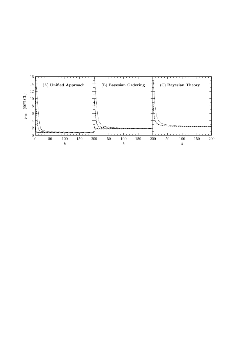
Figure 8: 90% CL upper limit $\mu_{\mathrm{up}}$ as a function of the background $b$ for $n=0$ (solid lines), $n=5$ (dashed lines) and $n=10$ (dotted lines).

Criticism: For $n=0$ the upper limit $\mu_{\mathrm{up}}$ should be independent of the background $b$.

But for $n>0$ the upper limit $\mu_{\mathrm{up}}$ always decreases with increasing $b$! It is true that for $n=0$ one is sure that no background event as well as no signal has been observed. But this is just the effect of a low fluctuation of the background that is present! Should we built a special theory for $n=0$? I think that this is not interesting in the Frequentist framework, because I guess that it leads necessarily to a violation of coverage (that could be tolerated, but not welcomed, only if it is overcoverage).

I think that if one is so interested in having an upper limit $\mu_{\mathrm{up}}$ independent of the background $b$ for $n=0$, one better embrace the Bayesian theory (see Fig. 3C, Fig. 8C and Ref. [14]), which, by the way, may present many other attractive qualities (see, for example, [1]).

Criticism: A (worse) experiment with larger background $b$ should not give a smaller upper limit $\mu_{\mathrm{up}}$ for the same number $n$ of observed events.

But, as shown in Fig. 3, this always happens! Notice that it happens both for $n>b$ (dotted part of lines) and for $n\leq b$ (solid part of lines), in Frequentist methods as well as in the Bayesian Theory (for $n>0$). As far as I know, nobody questions the decrease of $\mu_{\mathrm{up}}$ as $b$ is increased if $n>b$. So why should we question the same behavior when $n\leq b$? The reason for this behavior is simple: the observation of a given number $n$ of observed events has the same probability if the background is small and the signal is large or the background is large and the signal is small.

I think that it is physically desirable that and experiment with a larger background do not give a much smaller upper limit for the same number of observed events, but a smaller upper limit is allowed by statistical fluctuation. Indeed,

upper limits (as confidence intervals, etc.) are statistical quantities that must fluctuate!

I think that the current race of experiments to find the most stringent upper limit is bad, because it induces people to think that limits are fixed and certain. Instead, everybody should understand that

a better experiment can sometimes give a worse upper limit because of statistical fluctuations and there is nothing wrong about it!

7 Conclusions

In this report I have shown that the necessity to choose a specific Frequentist method, among several available, does not introduce any degree of subjectivity from a statistical point of view (Section 2) [6]. In other words, all Frequentist methods are statistically equivalent.

However, the physical significance of confidence intervals obtained with different methods is different and scientists interested in obtaining reliable and useful information on the characteristics of the real world must worry about this problem. Obtaining empty or very small confidence intervals for a physical quantity as a result of a statistical procedure is useless. Sometimes it is even dangerous to present such results, that lead non-experts in statistics (and sometimes experts too) to false believes.

In Section 3 I have discussed some virtues and shortcomings of the Unified Approach [7]. These shortcomings are ameliorated in the Bayesian Ordering method [8], discussed in Section 5, that is natural, relatively easy, and leads to more reliable upper limits.

In conclusion, I would like to emphasize the following considerations:

• One must always remember that, in order to have coverage, the choice of a specific Frequentist method must be done independently of the knowledge of the data.

• Finding some examples in which a method fails does not imply that it should not be adopted in the cases in which it performs well.

• Since all Frequentist methods are statistically equivalent,

  there is no need of a general Frequentist method!

  In each case one can choose the method that works better (basing the judgment on easiness, meaningfulness of limits, etc.). Complicated methods with a wider range of applicability are theoretically interesting, but not attractive in practice.

• Somebody thinks that the physics community should agree on a standard statistical method (see, for example, [15]). In that case, it is clear that this method must be always applicable. But this is not the case, for example, of the Unified Approach, as shown in [16]. Although the Bayesian Ordering method has not been submitted to a similar thorough examination, I doubt that it is generally applicable.

  I do not see why experiments that explore different physics and use different experimental techniques should all use the same statistical method (except a possible ignorance of statistics and blind believe to “authorities”).

  I would recommend that

  instead of wasting time on useless characteristics as generality, the physics community should worry about the usefulness and credibility of experimental results.

References

- [1] G. D’Agostini, CERN Yellow Report 99-03 (available at http://www-zeus.roma1.infn.it/%7Eagostini/prob+stat.html); Am. J. Phys. 67, 1260 (1999) [arXiv:physics/9908014]; arXiv:physics/9906048.
- [2] Philos. Trans. R. Soc. London Sect. A 236, 333 (1937), reprinted in A selection of Early Statistical Papers on J. Neyman, University of California, Berkeley, 1967, p. 250.
- [3] W.T. Eadie, D. Drijard, F.E. James, M. Roos and B. Sadoulet, Statistical Methods in Experimental Physics, North Holland, Amsterdam, 1971.
- [4] R.D. Cousins, Am. J. Phys. 63, 398 (1995).
- [5] C. Giunti, Phys. Rev. D 59, 113009 (1999) [arXiv:hep-ex/9901015].
- [6] C. Giunti and M. Laveder, arXiv:hep-ex/0002020.
- [7] G.J. Feldman and R.D. Cousins, Phys. Rev. D 57, 3873 (1998) [arXiv:physics/9711021].
- [8] C. Giunti, Phys. Rev. D 59, 053001 (1999) [arXiv:hep-ph/9808240].
- [9] S. Ciampolillo, Il Nuovo Cimento A 111, 1415 (1998).
- [10] B.P. Roe and M.B. Woodroofe, Phys. Rev. D 60, 053009 (1999) [arXiv:physics/9812036].
- [11] M. Mandelkern and J. Schultz, arXiv:hep-ex/9910041.
- [12] G. Punzi, arXiv:hep-ex/9912048.
- [13] C. Giunti, in Summary of the NOW’98 Phenomenology Working Group [arXiv:hep-ph/9906251].
- [14] P. Astone and G. Pizzella, these Proceedings [hep-ex/0002028].
- [15] “Panel Discussion” at this this Workshop (http://www.cern.ch/CERN/Divisions/EP/Events/CLW).
- [16] G. Zech, these Proceedings (http://www.cern.ch/CERN/Divisions/EP/Events/CLW).