EUROPEAN ORGANISATION FOR NUCLEAR RESEARCH

CERN-EP/99-175

13th December 1999

QCD Analyses and Determinations of $\alpha_{s}$ in ${\rm e}^{+}{\rm e}^{-}$ Annihilation at Energies between 35 and 189 GeV

The JADE (*) and the OPAL (**) Collaboration

Abstract:

We employ data taken by the JADE and OPAL experiments for an integrated QCD study in hadronic ${\rm e}^{+}{\rm e}^{-}$ annihilations at c.m.s. energies ranging from 35 GeV through 189 GeV. The study is based on jet-multiplicity related observables. The observables are obtained to high jet resolution scales with the JADE, Durham, Cambridge and cone jet finders, and compared with the predictions of various QCD and Monte Carlo models. The strong coupling strength, $\alpha_{s}$, is determined at each energy by fits of ${\cal O}(\alpha_{s}^{2})$ calculations, as well as matched ${\cal O}(\alpha_{s}^{2})$ and NLLA predictions, to the data. Matching schemes are compared, and the dependence of the results on the choice of the renormalization scale is investigated. The combination of the results using matched predictions gives

$$\alpha_{s}(M_{Z^{0}})=0.1187\raisebox{-3.01385pt}{$\stackrel{{\scriptstyle\textstyle+0.0034}}{{-0.0019}}$}.$$

The strong coupling is also obtained, at lower precision, from ${\cal O}(\alpha_{s}^{2})$ fits of the c.m.s. energy evolution of some of the observables. A qualitative comparison is made between the data and a recent MLLA prediction for mean jet multiplicities.

To be submitted to European Physical Journal C

P. Pfeifenschneider¹⁴, O. Biebel^14,i, P.A. Movilla Fernández^14,i and the members of the former JADE Collaboration who are fully listed in Ref. [1]

(**) The OPAL Collaboration

G. Abbiendi², K. Ackerstaff⁸, P.F. Akesson³, G. Alexander²², J. Allison¹⁶, K.J. Anderson⁹, S. Arcelli¹⁷, S. Asai²³, S.F. Ashby¹, D. Axen²⁷, G. Azuelos^18,a, I. Bailey²⁶, A.H. Ball⁸, E. Barberio⁸, R.J. Barlow¹⁶, J.R. Batley⁵, S. Baumann³, T. Behnke²⁵, K.W. Bell²⁰, G. Bella²², A. Bellerive⁹, S. Bentvelsen⁸, S. Bethke^14,i, O. Biebel^14,i, A. Biguzzi⁵, I.J. Bloodworth¹, P. Bock¹¹, J. Böhme^14,h, O. Boeriu¹⁰, D. Bonacorsi², M. Boutemeur³¹, S. Braibant⁸, P. Bright-Thomas¹, L. Brigliadori², R.M. Brown²⁰, H.J. Burckhart⁸, J. Cammin³, P. Capiluppi², R.K. Carnegie⁶, A.A. Carter¹³, J.R. Carter⁵, C.Y. Chang¹⁷, D.G. Charlton^1,b, D. Chrisman⁴, C. Ciocca², P.E.L. Clarke¹⁵, E. Clay¹⁵, I. Cohen²², O.C. Cooke⁸, J. Couchman¹⁵, C. Couyoumtzelis¹³, R.L. Coxe⁹, M. Cuffiani², S. Dado²¹, G.M. Dallavalle², S. Dallison¹⁶, R. Davis²⁸, A. de Roeck⁸, P. Dervan¹⁵, K. Desch²⁵, B. Dienes^30,h, M.S. Dixit⁷, M. Donkers⁶, J. Dubbert³¹, E. Duchovni²⁴, G. Duckeck³¹, I.P. Duerdoth¹⁶, P.G. Estabrooks⁶, E. Etzion²², F. Fabbri², A. Fanfani², M. Fanti², A.A. Faust²⁸, L. Feld¹⁰, P. Ferrari¹², F. Fiedler²⁵, M. Fierro², I. Fleck¹⁰, A. Frey⁸, A. Fürtjes⁸, D.I. Futyan¹⁶, P. Gagnon¹², J.W. Gary⁴, G. Gaycken²⁵, C. Geich-Gimbel³, G. Giacomelli², P. Giacomelli², D.M. Gingrich^28,a, D. Glenzinski⁹, J. Goldberg²¹, W. Gorn⁴, C. Grandi², K. Graham²⁶, E. Gross²⁴, J. Grunhaus²², M. Gruwé²⁵, P.O. Günther³, C. Hajdu²⁹ G.G. Hanson¹², M. Hansroul⁸, M. Hapke¹³, K. Harder²⁵, A. Harel²¹, C.K. Hargrove⁷, M. Harin-Dirac⁴, A. Hauke³, M. Hauschild⁸, C.M. Hawkes¹, R. Hawkings²⁵, R.J. Hemingway⁶, C. Hensel²⁵, G. Herten¹⁰, R.D. Heuer²⁵, M.D. Hildreth⁸, J.C. Hill⁵, P.R. Hobson²⁵, A. Hocker⁹, K. Hoffman⁸, R.J. Homer¹, A.K. Honma⁸, D. Horváth^29,c, K.R. Hossain²⁸, R. Howard²⁷, P. Hüntemeyer²⁵, P. Igo-Kemenes¹¹, D.C. Imrie²⁵, K. Ishii²³, F.R. Jacob²⁰, A. Jawahery¹⁷, H. Jeremie¹⁸, M. Jimack¹, C.R. Jones⁵, P. Jovanovic¹, T.R. Junk⁶, N. Kanaya²³, J. Kanzaki²³, G. Karapetian¹⁸, D. Karlen⁶, V. Kartvelishvili¹⁶, K. Kawagoe²³, T. Kawamoto²³, P.I. Kayal²⁸, R.K. Keeler²⁶, R.G. Kellogg¹⁷, B.W. Kennedy²⁰, D.H. Kim¹⁹, A. Klier²⁴, T. Kobayashi²³, M. Kobel³, T.P. Kokott³, M. Kolrep¹⁰, S. Komamiya²³, R.V. Kowalewski²⁶, T. Kress⁴, P. Krieger⁶, J. von Krogh¹¹, T. Kuhl³, M. Kupper²⁴, P. Kyberd¹³, G.D. Lafferty¹⁶, H. Landsman²¹, D. Lanske¹⁴, I. Lawson²⁶, J.G. Layter⁴, A. Leins³¹, D. Lellouch²⁴, J. Letts¹², L. Levinson²⁴, R. Liebisch¹¹, J. Lillich¹⁰, B. List⁸, C. Littlewood⁵, A.W. Lloyd¹, S.L. Lloyd¹³, F.K. Loebinger¹⁶, G.D. Long²⁶, M.J. Losty⁷, J. Lu²⁷, J. Ludwig¹⁰, A. Macchiolo¹⁸, A. Macpherson²⁸, W. Mader³, M. Mannelli⁸, S. Marcellini², T.E. Marchant¹⁶, A.J. Martin¹³, J.P. Martin¹⁸, G. Martinez¹⁷, T. Mashimo²³, P. Mättig²⁴, W.J. McDonald²⁸, J. McKenna²⁷, T.J. McMahon¹, R.A. McPherson²⁶, F. Meijers⁸, P. Mendez-Lorenzo³¹, F.S. Merritt⁹, H. Mes⁷, I. Meyer⁵, A. Michelini², S. Mihara²³, G. Mikenberg²⁴, D.J. Miller¹⁵, W. Mohr¹⁰, A. Montanari², T. Mori²³, K. Nagai⁸, I. Nakamura²³, H.A. Neal^12,f, R. Nisius⁸, S.W. O’Neale¹, F.G. Oakham⁷, F. Odorici², H.O. Ogren¹², A. Okpara¹¹, M.J. Oreglia⁹, S. Orito²³, G. Pásztor²⁹, J.R. Pater¹⁶, G.N. Patrick²⁰, J. Patt¹⁰, R. Perez-Ochoa⁸, P. Pfeifenschneider¹⁴, J.E. Pilcher⁹, J. Pinfold²⁸, D.E. Plane⁸, B. Poli², J. Polok⁸, M. Przybycień^8,d, A. Quadt⁸, C. Rembser⁸, H. Rick⁸, S.A. Robins²¹, N. Rodning²⁸, J.M. Roney²⁶, S. Rosati³, K. Roscoe¹⁶, A.M. Rossi², Y. Rozen²¹, K. Runge¹⁰, O. Runolfsson⁸, D.R. Rust¹², K. Sachs¹⁰, T. Saeki²³, O. Sahr³¹, W.M. Sang²⁵, E.K.G. Sarkisyan²², C. Sbarra²⁶, A.D. Schaile³¹, O. Schaile³¹, P. Scharff-Hansen⁸, J. Schieck¹¹, S. Schmitt¹¹, A. Schöning⁸, M. Schröder⁸, M. Schumacher²⁵, C. Schwick⁸, W.G. Scott²⁰, R. Seuster^14,h, T.G. Shears⁸, B.C. Shen⁴, C.H. Shepherd-Themistocleous⁵, P. Sherwood¹⁵, G.P. Siroli², A. Skuja¹⁷, A.M. Smith⁸, G.A. Snow¹⁷, R. Sobie²⁶, S. Söldner-Rembold^10,e, S. Spagnolo²⁰, M. Sproston²⁰, A. Stahl³, K. Stephens¹⁶, K. Stoll¹⁰, D. Strom¹⁹, R. Ströhmer³¹, B. Surrow⁸, S.D. Talbot¹, S. Tarem²¹, R.J. Taylor¹⁵, R. Teuscher⁹, M. Thiergen¹⁰, J. Thomas¹⁵, M.A. Thomson⁸, E. Torrence⁸, S. Towers⁶, T. Trefzger³¹, I. Trigger⁸, Z. Trócsányi^30,g, E. Tsur²², M.F. Turner-Watson¹, I. Ueda²³, R. Van Kooten¹², P. Vannerem¹⁰, M. Verzocchi⁸, H. Voss³, D. Waller⁶, C.P. Ward⁵, D.R. Ward⁵, P.M. Watkins¹, A.T. Watson¹, N.K. Watson¹, P.S. Wells⁸, T. Wengler⁸, N. Wermes³, D. Wetterling¹¹ J.S. White⁶, G.W. Wilson¹⁶, J.A. Wilson¹, T.R. Wyatt¹⁶, S. Yamashita²³, V. Zacek¹⁸, D. Zer-Zion⁸

¹School of Physics and Astronomy, University of Birmingham, Birmingham B15 2TT, UK
²Dipartimento di Fisica dell’ Università di Bologna and INFN, I-40126 Bologna, Italy
³Physikalisches Institut, Universität Bonn, D-53115 Bonn, Germany
⁴Department of Physics, University of California, Riverside CA 92521, USA
⁵Cavendish Laboratory, Cambridge CB3 0HE, UK
⁶Ottawa-Carleton Institute for Physics, Department of Physics, Carleton University, Ottawa, Ontario K1S 5B6, Canada
⁷Centre for Research in Particle Physics, Carleton University, Ottawa, Ontario K1S 5B6, Canada
⁸CERN, European Organisation for Particle Physics, CH-1211 Geneva 23, Switzerland
⁹Enrico Fermi Institute and Department of Physics, University of Chicago, Chicago IL 60637, USA
¹⁰Fakultät für Physik, Albert Ludwigs Universität, D-79104 Freiburg, Germany
¹¹Physikalisches Institut, Universität Heidelberg, D-69120 Heidelberg, Germany
¹²Indiana University, Department of Physics, Swain Hall West 117, Bloomington IN 47405, USA
¹³Queen Mary and Westfield College, University of London, London E1 4NS, UK
¹⁴Technische Hochschule Aachen, III Physikalisches Institut, Sommerfeldstrasse 26-28, D-52056 Aachen, Germany
¹⁵University College London, London WC1E 6BT, UK
¹⁶Department of Physics, Schuster Laboratory, The University, Manchester M13 9PL, UK
¹⁷Department of Physics, University of Maryland, College Park, MD 20742, USA
¹⁸Laboratoire de Physique Nucléaire, Université de Montréal, Montréal, Quebec H3C 3J7, Canada
¹⁹University of Oregon, Department of Physics, Eugene OR 97403, USA
²⁰CLRC Rutherford Appleton Laboratory, Chilton, Didcot, Oxfordshire OX11 0QX, UK
²¹Department of Physics, Technion-Israel Institute of Technology, Haifa 32000, Israel
²²Department of Physics and Astronomy, Tel Aviv University, Tel Aviv 69978, Israel
²³International Centre for Elementary Particle Physics and Department of Physics, University of Tokyo, Tokyo 113-0033, and Kobe University, Kobe 657-8501, Japan
²⁴Particle Physics Department, Weizmann Institute of Science, Rehovot 76100, Israel
²⁵Universität Hamburg/DESY, II Institut für Experimental Physik, Notkestrasse 85, D-22607 Hamburg, Germany
²⁶University of Victoria, Department of Physics, P O Box 3055, Victoria BC V8W 3P6, Canada
²⁷University of British Columbia, Department of Physics, Vancouver BC V6T 1Z1, Canada
²⁸University of Alberta, Department of Physics, Edmonton AB T6G 2J1, Canada
²⁹Research Institute for Particle and Nuclear Physics, H-1525 Budapest, P O Box 49, Hungary
³⁰Institute of Nuclear Research, H-4001 Debrecen, P O Box 51, Hungary
³¹Ludwigs-Maximilians-Universität München, Sektion Physik, Am Coulombwall 1, D-85748 Garching, Germany

^a and at TRIUMF, Vancouver, Canada V6T 2A3
^b and Royal Society University Research Fellow
^c and Institute of Nuclear Research, Debrecen, Hungary
^d and University of Mining and Metallurgy, Cracow
^e and Heisenberg Fellow
^f now at Yale University, Dept of Physics, New Haven, USA
^g and Department of Experimental Physics, Lajos Kossuth University, Debrecen, Hungary
^h and MPI München
ⁱ now at MPI für Physik, 80805 München.

1 Introduction

The renormalized strong coupling strength $\alpha_{s}$ of quantum chromodynamics (QCD) is predicted to depend upon the momentum transfer of the interaction under study. It is desirable to perform tests of QCD at different values of this momentum scale. These tests are best performed using uniform experimental conditions since systematic uncertainties may thereby be reduced. Until recently, rather limited sets of definite c.m.s. energies were available for QCD analyses in ${\rm e}^{+}{\rm e}^{-}$ collisions under consistent conditions. Since the start of the “LEP 2” program in 1995, the c.m.s. energy of the LEP collider at CERN has been increased in several steps from its original values close to 91.2 GeV, allowing QCD analyses over a wide range of high c.m.s. energies. However, the inclusion of measurements at lower c.m.s. energies is important as well, because QCD becomes more strongly dependent on the energy scale towards lower energies, and tests of the theory will be most significant here.

This paper presents QCD tests using ${\rm e}^{+}{\rm e}^{-}$ annihilations into hadrons (so-called multihadronic events) from $\sqrt{s}=35$ GeV to 189 GeV. Data recorded at the OPAL experiment at LEP are analyzed in combination with data from the JADE experiment at the PETRA collider at DESY, where ${\rm e}^{+}{\rm e}^{-}$ collisions were studied from 1978 to 1986 at lower c.m.s. energies. The OPAL and JADE detectors are similar in construction, and we have tried to keep the experimental procedure in both analyses as similar as possible.

The observables used are exclusively based on the multiplicities of hadronic jets, defined using standard techniques. In the first part of the present work we present measurements of a large variety of such observables and compare them with several Monte Carlo predictions. The measurements are then employed to determine the strong coupling strength $\alpha_{s}$ and to test the QCD prediction for the momentum transfer dependence, i.e. the “running,” of $\alpha_{s}$. We compare the results from different types of matched ${\cal O}(\alpha_{s}^{2})$ and NLLA predictions as well as pure ${\cal O}(\alpha_{s}^{2})$ predictions and study the dependence of the fit results on the renormalization scale. The individual results are combined into a final value for $\alpha_{s}(M_{Z^{0}})$. Finally, a recent MLLA calculation for the mean jet multiplicity is compared with our measurements without extracting a value for $\alpha_{s}$.

	$\sqrt{s}$ ($\langle\sqrt{s}\rangle$)	period of	integrated	number of
	[GeV]	data taking	luminosity [pb-1]	selected events
J	(34.6)	1982	37.5	8721
A	34.5–35.5 (35.0)	1986	92.3	20793
D
E	43.4–44.3 (43.7)	1984/85	30.3	4110
	91.2	1994	34	1508031
	130		2.6	144
O	136	1995	2.5	140
P	130		2.6	179
A	136	1997	3.3	167
L	161	1996	10.0	281
	172	1996	10.42	224
	183	1997	55.22	1082
	189	1998	186.3	3300

Table 1: Overview of the data samples used in this analysis. The quoted numbers of selected events refer to the standard selection so described in Sect. 3. For the c.m.s. energies of the JADE experiment, the mean value $\langle\sqrt{s}\rangle$, averaged over the selected events, is given in parentheses. The small difference between the event number at $\sqrt{s}=35$ GeV and that given in [6] is due to a somewhat more stringent definition of “long tracks” (see table 7) in this analysis.

2 The Experiments

The ${\rm e}^{+}{\rm e}^{-}$ storage ring PETRA (see e.g. [2]) was operated for physics measurements from 1978 until 1986 at c.m.s. energies ranging from 12 GeV to 46.7 GeV. Extensive energy scans were made between these values. This analysis uses data samples recorded at energies of $\sqrt{s}=35$ and 44 GeV. The precise ranges in c.m.s. energy and the luminosities are given in Table 1.

The LEP ${\rm e}^{+}{\rm e}^{-}$ collider at CERN began operation in 1989 at $\sqrt{s}\approx 91$ GeV, i.e. around the mass of the $Z^{0}$ boson. Since Fall 1995, the energy has been increased in steps from 130 GeV, 136 GeV, 161 GeV, 172 GeV, 183 GeV to 189 GeV in 1998, the last year for which we include data in this study. The luminosities recorded by the OPAL experiment at each of these energies are also listed in Table 1.

Descriptions of the JADE and OPAL detectors can be found in [1, 3] and [4], respectively. Apart from the dimensions, the detectors are very similar in their construction. Both are multi-purpose devices with a large solid angle coverage. Table 2 summarizes some detector parameters. The $r$, $\phi$ and $z$ coordinates refer to a cylindrical coordinate system with the origin lying in the center of the detector and the $z$ axis pointing along the incoming electron beam direction.

The detector components primarily used in this analysis are the tracking systems and the electromagnetic calorimeters. The main parts of the tracking systems of both detectors are drift chambers built with a “jet chamber” geometry. The relative resolution of the transverse track momentum can be parameterized as $\sigma(p_{t})/p_{t}=\sqrt{A_{t}^{2}+(B_{t}\cdot p_{t}\left[GeV\right])^{2}}$. The values of $A_{t}$ and $B_{t}$ for JADE and OPAL are given in Table 2.

The electromagnetic calorimeters (ECAL) of JADE and OPAL are arrays of lead-glass blocks. The relative resolution of the electromagnetic cluster energy $E$ is $\sigma(E)/E=A_{c}+B_{c}/\sqrt{E\left[GeV\right]}$. The parameters $A_{c}$ and $B_{c}$ are given in Table 2 for both detectors.

	Parameter			JADE	OPAL
	overall length			8 m	12 m
Dimensions	overall height			7 m	12 m
		length		2.4 m	4 m
	dimension	outer radius		0.8 m	1.85 m
	transv. momentum		$A_{t}$	0.04	0.02
	resolution $\sigma(p_{t})/p_{t}$		$B_{t}$	0.018	0.0015
	spatial		$r-\phi$	180 $\mu$m (110 $\mu$m)	135 $\mu$m
	resolution		$z$	1.6 cm	4.5—6 cm
	double hit resolution			7.5 mm (2 mm)	2.5 mm
Tracking	gas composition
system	argon/methane/isobutane			88.7%/8.5%/2.8%	88%/9.4%/2.6%
	gas pressure			4 bar	4 bar
	max. no. of hits			48	159
	reachable in			$0.83\cdot 4\pi$	$0.73\cdot 4\pi$
	at least 8 hits
	reachable in			$0.97\cdot 4\pi$	$0.98\cdot 4\pi$
	magnetic field			0.48 T	0.435 T
	energy		$A_{c}$	0.015	0.002
	resolution $\sigma(E)/E$		$B_{c}$	0.04	0.063
	solid angle coverage			90%	98%
	angular resolution			7 mrad	2 mrad
		radial extent		1—1.4 m	2.5—2.8 m
Electromagnetic		length		3.6 m	7 m
calorimetry	barrel	polar angle covered		$32^{\circ}$–$148^{\circ}$	$36^{\circ}$–$144^{\circ}$
		radiation depth		12.5$X_{0}$ (15.7$X_{0}$)	24.6$X_{0}$
		granularity		8.5$\times$10 cm2	10$\times$10 cm2
		outer radius		0.9 m	1.8 m
	endcap	polar angle covered		$11^{\circ}$–$32^{\circ}$/$148^{\circ}$–$169^{\circ}$	$11^{\circ}$–$36^{\circ}$/$144^{\circ}$–$169^{\circ}$
		radiation depth		9.6$X_{0}$	22$X_{0}$
		granularity		14$\times$14 cm2	9$\times$9 cm2

Table 2: Parameters of the JADE and OPAL detectors are compiled from [1, 3, 4, 5]. Wherever a second number is given in parentheses, it refers to a later period of detector operation. The significance of the parameters $A_{t}$, $B_{t}$, $A_{c}$ and $B_{c}$ is described in the text.

3 Data Samples and Multihadronic Event Selection

In the JADE part of the analysis we use “detector level” information from data and Monte Carlo samples as described in [6], obtained from (measured or simulated) detector signals before any corrections are applied. We use data from the 1982 and 1986 runs at $\sqrt{s}=35$ GeV and the 1985 runs at 44 GeV, where Monte Carlo samples including detector level information are available. It was shown in previous reanalyses of JADE data [6, 7] that measurements made in 1986 and before could be reproduced using these data and Monte Carlo samples.

At $\sqrt{s}=M_{Z^{0}}$, we use the complete OPAL run of 1994 which is the largest available homogeneous run without changes in the OPAL experimental set-up.

From the first runs at higher c.m.s. energies in 1995 we combine the two samples at $\sqrt{s}=130$ and 136 GeV, weighting them with their statistical errors. Runs in 1997 at the same two c.m.s. energies are used as well and subjected to the same treatment. The runs from 1995 and 1997 are analyzed independently of each other since changes of the detector were made between the two dates. In both cases, results are quoted at $\sqrt{s}=133$ GeV. For each of the following energy steps we use the full event samples recorded by OPAL and quote results for the respective averaged c.m.s. energies.

In order to reject lepton pairs and two-photon collisions, we apply standard selections from the two experiments. The selection used for the JADE part of the analysis is the same as described in [6] and [8], and is closely related to that of OPAL, taking into account the difference in c.m.s. energies. For the OPAL analysis we apply the criteria given in [9]. Table 3 contains a comparative list of the most important cuts used for the JADE and the OPAL analyses. We shall refer to this set of cuts as the “preselection”.

At c.m.s. energies above $M_{Z^{0}}$, photon radiation in the initial state becomes a significant source of background. In order to reject such “ISR events” we determine the total hadronic mass $\sqrt{s^{\prime}}$ of an event following a procedure based on that described in [10] which takes possible multiple photon radiation into account. We require events to have $\sqrt{s}-\sqrt{s^{\prime}}<10\;\mbox{GeV}$. For systematics studies we apply alternatively a combination of cuts on the visible energy and missing momentum of the event and on the energy of an isolated photon candidate [11]. We shall refer to the former procedure as the “invariant mass” selection and to the latter as the “energy balance” selection.

Reaction to be
suppressed	Cut variable	JADE	OPAL
2-lepton		$\geq 3$ long tracks
events	$n_{ch}$	and $\geq 4$ central tracks	$\geq 7$
	$n_{cal}$	—	$\geq 7$
		$>3.0$ GeV (barrel)
	$E_{shw}$	or $>0.4$ GeV (per endcap)	—
2-photon	$E_{vis}/\sqrt{s}$	$>0.5$	$>0.1$
events	$p_{bal}$	$<0.4$	$<0.6$
	$p_{miss}$	$0.3\cdot\sqrt{s}$	—
other	$|\cos{\theta_{T}}|$	$<0.8$	$<0.9$

Table 3: Comparison of the preselection cut values against two-lepton and two-photon events for the JADE and OPAL experiments. $n_{ch}$, $n_{cal}$ and $E_{shw}$ denote, respectively, the number of charged tracks and calorimeter clusters and the total shower energy deposited in the calorimeters. $E_{vis}$ is the total visible energy, $p_{miss}$ the total missing momentum and $p_{bal}$ the momentum sum in $z$ direction, normalized by $E_{vis}$. Both experiments also apply cuts on the polar angle of the thrust axis, $\theta_{T}$. The terms “long” and “central tracks” are explained in Table 7 in Appendix A.

At $\sqrt{s}=161$ GeV and above, the production of $W^{\pm}$ (and later also $Z^{0}$) pairs with hadronic decays is another source of background. At these higher energies, we reject such reactions by dividing each event into hemispheres using the plane perpendicular to the thrust axis [12]. We denote the heavier and lighter invariant mass of each hemisphere, normalized with the visible energy, by $M_{H}$ and $M_{L}$ [13]. Events with weak boson pairs decaying hadronically usually have larger hemisphere invariant masses. We apply the cut $M_{H}/2+M_{L}<0.35$ and refer to this as the “jet mass selection”. An alternative selection method has been used in previous OPAL analyses (e.g. [14]): the event is resolved into four jets using the Durham jet finder, and the ${\cal O}(\alpha_{s}^{2})$ QCD matrix element for a four-parton final state is calculated using the jet four-momenta $p_{1}$…$p_{4}$. The value of the matrix element is used as a cut variable. This method will be called the “event weight selection” and serves as a systematic check. The jet mass and event weight selections have very similar performance when applied to a sample of Monte Carlo events from PYTHIA [15] (for multihadronic events) and GRC4F [16] (for all relevant four-fermion processes) which have been passed through the preselection and the invariant mass selection.

Table 1 lists the numbers of events which we select at the individual c.m.s. energies using the standard selections.

4 Measurement of Jet Fractions

We present measurements of jet-multiplicity related quantities for various jet finders at c.m.s. energies of 35 through 189 GeV and compare them with predictions of several Monte Carlo models. The measured quantities are corrected for effects of limited detector resolution and acceptance, as well as for inefficiencies of the selection and ISR, i.e. they are presented at the “hadron level,” which is understood to include all charged and neutral particles emerging after all intermediate particles with lifetimes below $3\cdot 10^{-10}$ s have decayed.

4.1 General Analysis Procedure

4.1.1 Reconstruction of Single Particles

For both experiments, the measurements are based on charged tracks and electromagnetic calorimeter clusters. From these the four-vectors of single particles are reconstructed according to techniques which are quite similar in both the JADE and the OPAL part of the analysis. After imposing the quality criteria for charged tracks and electromagnetic calorimeter clusters described in Appendix A, each accepted track is regarded as a charged particle having the measured three-momentum of the track and the mass of a charged pion. If a track can be linked to a particular ECAL cluster an estimate is made of the energy which a charged pion would deposit in the calorimeter; this amount is subtracted from the energy of the cluster. If the entire cluster energy is used up by such subtractions, the cluster is discarded; otherwise, the remaining energy is assumed to have been deposited by an additional neutral particle, and a zero-mass four-vector is constructed from this energy and the position of the cluster.

The set of four-vectors from each selected event is then passed to the jet algorithms. At those c.m.s. energies where initial state photon radiation is large ($\sqrt{s}=133$ GeV and higher), the entire system of vectors is boosted into its own rest frame before the algorithms are applied.

4.1.2 Correction for Experimental Effects

At the c.m.s. energies of the JADE experiment (35 and 44 GeV), corrections rely on existing Monte Carlo samples with full detector simulation, taking into account the changes of the detector with time. The detector level Monte Carlo samples available for this analysis were generated using the JETSET 6.3 program [17] with the standard parameter set of the JADE collaboration [18] and including photon radiation in the initial state. The Monte Carlo samples were shown in previous publications [6, 7] to describe the data well. They were processed in the same way as the data, i.e. subjected to the same selection cuts and single particle reconstruction procedures.

To obtain the corresponding hadron level information we have run the JETSET 6.3 program to generate events at both c.m.s. energies, using the same parameter settings, but without initial state photon radiation. By dividing the hadron level by the detector level prediction, binwise multiplicative correction factors were determined for all observables and then applied to the data.

A similar binwise multiplicative correction procedure is applied to the OPAL data at $\sqrt{s}=91$ GeV. The correction factors were determined from two distinct Monte Carlo samples with detector simulation, generated by JETSET 7.4 [19] and HERWIG 5.9 [20]. The parameter settings for both generators are described in [10, 21]. Initial and final state photon radiation is included in both cases.

For c.m.s. energies of 133 GeV and above, the JETSET Monte Carlo is replaced by PYTHIA 5.7 [15], which has a more accurate modelling of initial state photon radiation. In addition, versions 5.8d (at $\sqrt{s}=161$ GeV) and 5.9 (otherwise) of HERWIG were used to generate multihadronic events. The correction procedure for ISR and detector effects applied at energies of 133 GeV and above was the same as at the lower c.m.s. energies.

At $\sqrt{s}=161$ GeV and above, all relevant four-fermion final states were generated by the GRC4F generator [16] and subjected to detector simulation. The background predicted by GRC4F for each observable is subtracted at the detector level before the multiplicative corrections for residual ISR background and detector effects are applied.

4.1.3 Determination of Systematic Errors

To assess the size of systematic uncertainties inherent to the analysis procedure, the entire analysis was repeated with variations of the selection, of the correction Monte Carlo generators and of the detector components used. For each variation, the deviation of the final result from the standard measurement is taken as a systematic uncertainty. All systematic uncertainties are added quadratically to yield the total systematic error for every bin of each variable.

The influence of the detector components used for the single particle reconstruction (tracking chambers and electromagnetic calorimeter) is estimated by repeating the analysis using only charged tracks. As a consistency check, where there are data sets from two different run periods ($\sqrt{s}=35$ GeV or 133 GeV), the influence of changes in the detectors carried out between the two dates has been investigated, but no effects were found.

A systematic variation of the selection mechanism is done at all energies by tightening the cut on the thrust axis from $|\cos{\theta_{T}}|<0.9$ to $|\cos{\theta_{T}}|<0.7$. In addition, at $\sqrt{s}=35$ GeV and 44 GeV, the cut variations described in [6] are performed: The cut on the total missing three-momentum $p_{miss}$ is either tightened from $0.3\cdot\sqrt{s}$ to $0.25\cdot\sqrt{s}$ or removed; the upper limit on the energy balance in beam direction, $p_{bal}$, is either tightened from 0.4 to 0.3 or removed; the cut on the normalized visible energy $E_{vis}/\sqrt{s}$ is varied from 0.5 to 0.55 and 0.45; a minimum of 7 rather than 3 “long tracks” (as defined in Appendix A) is demanded. For the analysis at $\sqrt{s}=91$ GeV, no further cross-checks aside from the variation of the thrust axis cut are done. At $\sqrt{s}=133$ GeV and above, the influence of the standard invariant mass selection is tested by replacing it by the energy balance selection, and at c.m.s. energies of 161 GeV and higher, the analysis is repeated using the event weight selection rather than the standard jet mass selection.

A variation of the correction Monte Carlo is not possible at JADE energies because no detector level samples aside from the ones used are currently available. At all other energies ($\sqrt{s}\geq 91$ GeV), the analysis is repeated using HERWIG for the determination of the corrections instead of JETSET or PYTHIA. The effect of using the EXCALIBUR generator [22] rather than GRC4F for the background has also been investigated. The deviation from the main result induced by this change was found to be negligible throughout and is therefore not added as an additional uncertainty.

Any systematic variation of the analysis procedure involving changes in the number of events entering the measurement of some numerical value (e.g. some bin) will necessarily generate a statistical deviation from the standard value. This effect becomes significant at c.m.s. energies with low statistics, i.e. at $\sqrt{s}=133$ GeV, 161 GeV and 172 GeV. To obtain a more realistic estimate of the systematic errors at these c.m.s. energies a number of subsamples are created from the respective multihadronic Monte Carlo sample, all of which contain on average the number of events corresponding to the integrated luminosity of the data (cf. [10]). Each of these subsamples is subjected to the same analysis procedure as the data. The standard deviation $\sigma$ of each separate contribution to the systematic error over all subsamples is determined for all measured values and regarded as the statistical component of the systematic error. If $\sigma$ is smaller than the corresponding systematic error contribution $\delta$ measured from the data, the latter is reduced to $\sqrt{\delta^{2}-\sigma^{2}}$. Otherwise, the respective contribution to the systematic error is dropped completely. The procedure is performed separately for each contribution to the systematic error before they are added. The number of Monte Carlo subsamples used is 16 for the 1995 run at 133 GeV and 30 in all other cases.

In order to further reduce fluctuations of the errors between measured values in adjacent bins due to low statistics, the overall systematic errors in all except the extreme bins of each quantity shown are averaged over each three adjacent values of that quantity. The systematic errors of the first and the last bin are subsequently set to the averaged errors of the three first and three last bins, respectively. This method of averaging systematic errors is performed at all c.m.s. energies.

4.2 Description of the Measured Jet Fractions

In the following, measurements are shown for three representative c.m.s. energy values: 35, 91 and 189 GeV. All quantities are plotted versus the parameter(s) of the respective jet algorithm. Error bars represent the quadratic sum of systematic and statistical uncertainties. The latter include effects of limited statistics of the data and of the correction Monte Carlo samples. Listings of the numerical values, including those for the c.m.s. energies which are not shown in the figures, are to appear in the Durham data base [23].

In each plot, the measurements are compared with hadron level predictions from the generators PYTHIA 5.722, HERWIG 5.9, ARIADNE 4.08 [24] and COJETS 6.23 [25], representing different kinds of parton shower and hadronization modelling. The parameter settings for ARIADNE and COJETS are those from [24] and [26]. The predictions are based on samples of multihadronic events without initial state photon radiation, generated independently of those used for the corrections. In the ARIADNE samples, initial states generated by PYTHIA were subjected to the ARIADNE parton shower simulation, in which the hadronization modelling was taken over from JETSET 7.408.

4.2.1 $n$-Jet Fractions

JADE Scheme

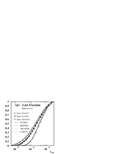
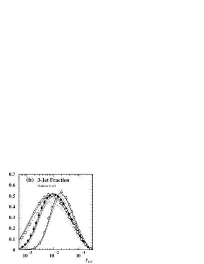
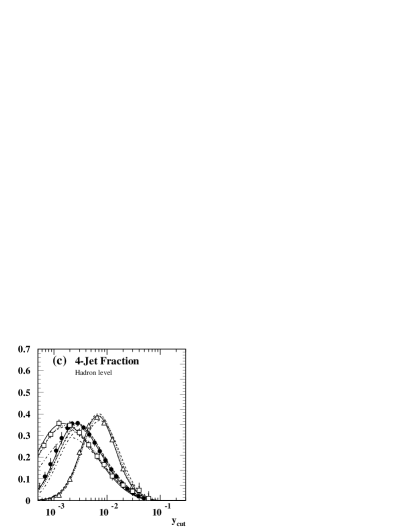
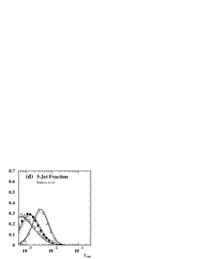
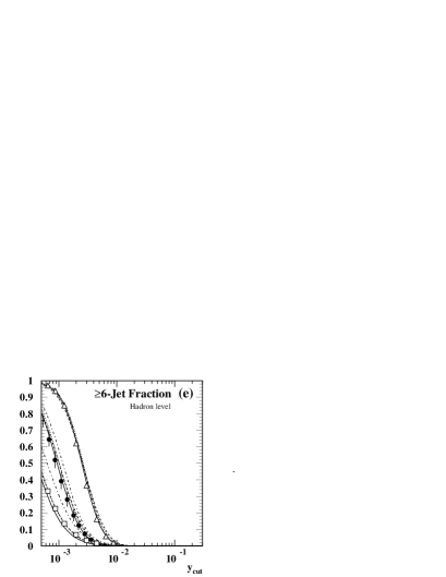
Figure 1: The fractions of events with 2, 3, 4, 5 and more than 5 jets as obtained by the JADE jet algorithm are plotted versus $y_{cut}$ at 35, 91 and 189 GeV. Data points are the measurements by the JADE and OPAL experiments. The error bars represent the total errors. Predictions by PYTHIA, HERWIG, ARIADNE and COJETS are shown using lines of different styles.

We analyze $n$-jet fractions, $R_{n}$, from the JADE [27], Durham [28] and Cambridge [29] jet finders, which reconstruct hadron jets based on different resolution parameters $y_{cut}$ and different procedures to recombine unresolvable jets. Measurements for $n=2$ through $n=5$ and $n\geq 6$ are shown versus $y_{cut}$ in Fig. 1, and in the upper and lower plots of Figs. 2 and 3, respectively. For each variable, the measurements at the three c.m.s. energies are combined in one plot to make changes with energy more visible. The same ranges in abscissa and ordinate were chosen for all c.m.s. energies within one scheme. We also use a cone jet finder.

At the highest c.m.s. energies, systematic effects due to hadronization are smallest. At $\sqrt{s}=35$ GeV and 44 GeV no HERWIG samples were available for the evaluation of the model uncertainties. Thus the apparent systematic errors are largest for the 91 GeV sample. The predictions of PYTHIA, HERWIG and ARIADNE are similar and lie mostly within the uncertainties of the measurements over the range in $y_{cut}$ studied. It is impossible to choose a clear best generator from these three. Since measurements of jet fractions for neighboring $y_{cut}$ values are partially based on the same events, the single bins of each jet fraction are strongly correlated.

The predictions of COJETS are also in many cases in agreement with the data. However, especially at higher c.m.s. energies ($\sqrt{s}\gtrsim 133$ GeV), too many jets are predicted in the low $y_{cut}$ regions. This is likely to be a consequence of the neglect of gluon coherence in the COJETS generator which may lead to an increased number of soft gluons between jets and therefore to high jet multiplicities. Coherence effects have already been observed by OPAL [30].

Scaling violations of both the Monte Carlo predictions and the measurements with $\sqrt{s}$ are visible for all three schemes in form of a reduction of the jet fractions for $n\geq 3$ (and a corresponding increase of $R_{2}$) at higher $\sqrt{s}$, as is expected from the running of $\alpha_{s}$ according to QCD. The resolution parameters $y_{cut}$ are defined in such a way that no scaling violations would be expected for jet rates if $\alpha_{s}$ did not run.

Fig. 4 displays $n$-jet fractions obtained with a cone jet finder described in [31], which reconstructs jets within cones of half angle $R$ having a minimum energy $\epsilon$. Because of the explicit energy cut inherent in the algorithm, results of the jet finding will depend strongly on the total energy $E_{vis}$ of the input particles. In order to remove this dependence, the cone algorithm is run with the scaled energy cut $\epsilon^{\prime}\equiv\epsilon\cdot E_{vis}/\sqrt{s}$. In the upper part of the figure, jet fractions are plotted versus $R$ for $n\leq 2$, $n=3$ and $n\geq 4$ at a fixed minimum jet energy $\epsilon$. A value of $\epsilon=7$ GeV is chosen for $\sqrt{s}=91$ GeV and above. At $\sqrt{s}=35$ GeV and 44 GeV, where typical jet energies are considerably lower, $\epsilon$ is set to 2.5 GeV and 3 GeV. The same jet fractions are shown against $\epsilon$ in the lower part of the figures, where $R$ is kept fixed at 0.7 rad.

As in the case of the clustering algorithms, the predictions of all Monte Carlo programs except that of COJETS are similar for all c.m.s. energies. Again, COJETS deviates from them and from the data above $\sqrt{s}=91$ GeV.

Durham Scheme

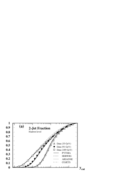
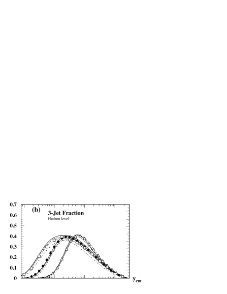
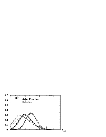
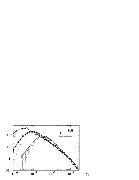
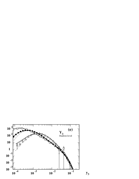
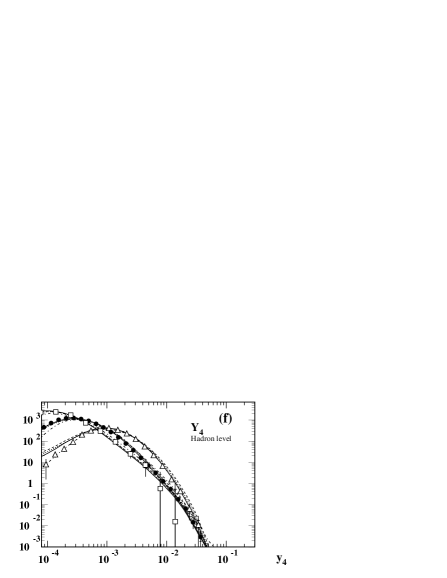
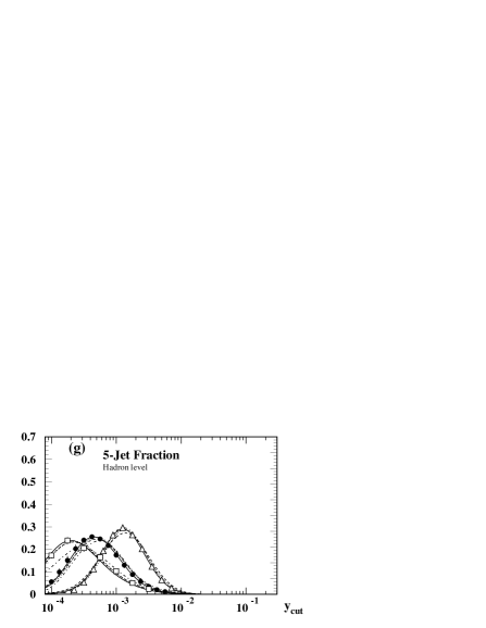
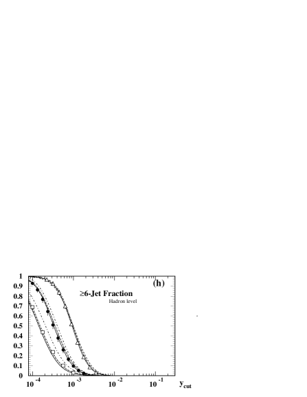
Figure 2: In plots (a), (b), (c), (g) and (h), the fractions of events with 2, 3, 4, 5 and more than 5 jets as obtained by the Durham scheme are plotted versus $y_{cut}$ at 35, 91 and 189 GeV. Diagrams (d) through (f) show the distributions in $y_{n}$ (see Sect. 4.2.2) corresponding to (a), (b) and (c). The presentation is the same as in Fig. 1. Small horizontal ticks indicate the size of the statistical errors.

Cambridge Scheme

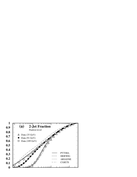
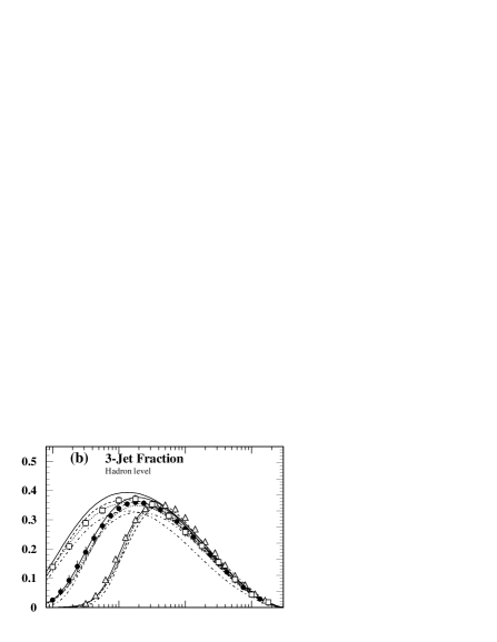
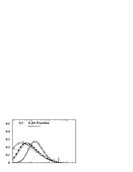
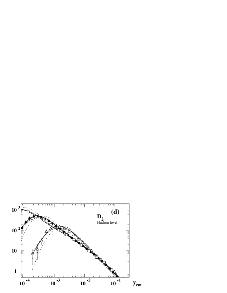
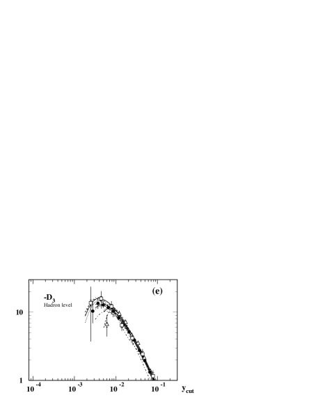
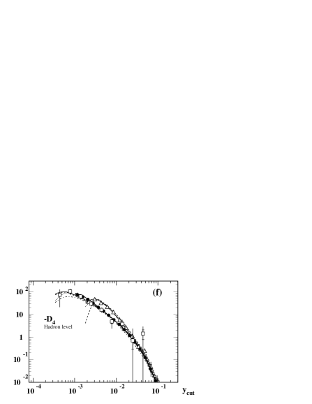
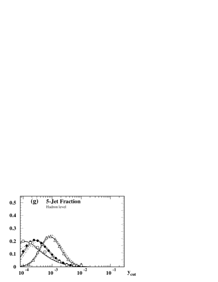
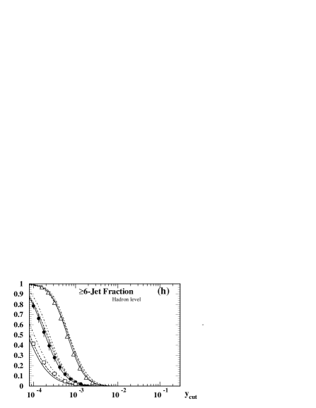
Figure 3: In plots (a), (b), (c), (g) and (h), jet fractions as obtained by the Cambridge scheme are plotted versus $y_{cut}$ at 35, 91 and 189 GeV as in Fig. 2. Diagrams (d) through (f) show the differential jet fractions $D_{n}$ (see section 4.2.2) corresponding to (a), (b) and (c).

Cone Algorithm

           

                 

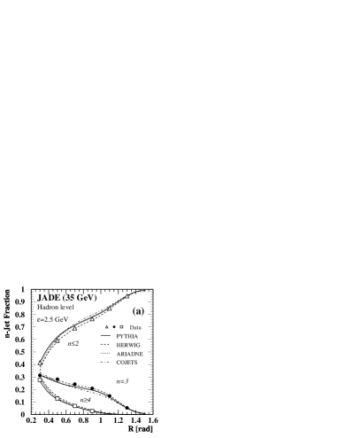
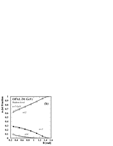
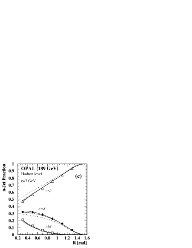
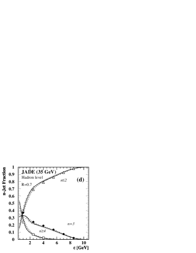
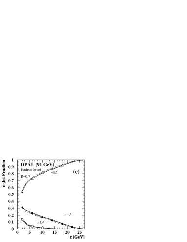
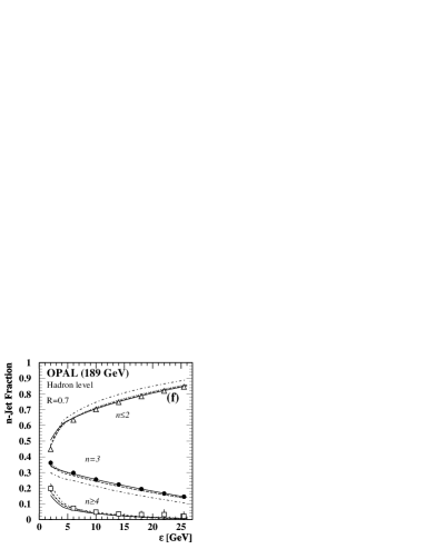
Figure 4: The fractions of events with 2 or less, 3 and more than 3 jets as obtained by the cone algorithm are plotted in the upper row versus the cone half angle $R$ at 35, 91 and 189 GeV, the jet energy cut-off $\epsilon$ being fixed at 2.5 GeV for $\sqrt{s}$=35 GeV or 7 GeV otherwise. The lower plots show the corresponding fractions versus $\epsilon$ with $R$ kept fixed at 0.7 rad. Data and Monte Carlo predictions are presented in the same form as in figures 1 through 3.

4.2.2 $y_{n}$ Distributions and Differential $n$-Jet Fractions

In the context of the JADE and Durham schemes, we shall denote by $y_{n}$ the value of $y_{cut}$ at which a particular event switches from a $n$-jet to an $n+1$-jet configuration. Any one of the quantities $y_{n}$ can be regarded as an event shape variable. We write differential distributions in $y_{n}$ as

$$Y_{n}\equiv\frac{1}{\sigma}\frac{\mbox{d}\sigma}{\mbox{d}y_{n}},$$ (1)

where $\sigma$ denotes the total hadronic cross section. In comparisons with theory, statistical correlations between the values at different parameter settings have to be taken into account. Such correlations are certainly present in $n$-jet fractions since the measurements at neighboring parameter values contain partially the same events. In this respect, the differential distributions $Y_{n}$ are more convenient quantities since they contain each event only once. In the middle row of Fig. 2 we present distributions $Y_{n}$ as obtained from the Durham scheme for $n=2$ through 4.

The Cambridge scheme employs a more complicated procedure for the jet reconstruction than the JADE and Durham schemes, involving two distinct resolution measures. There is therefore no counterpart of the quantities $y_{n}$ in the Cambridge scheme which would allow the interpretation described above (see e.g. [32, 33]). We show instead, in the middle row of Fig. 3, the corresponding “differential $n$-jet fractions,”

$$D_{n}\equiv\frac{1}{\sigma}\frac{\mbox{d}\sigma_{n}}{\mbox{d}y_{cut}},$$ (2)

with $\sigma_{n}$ being the cross section for the production of $n$ jets determined from explicit binwise differentiation of the jet fractions. The relation $D_{n}=Y_{n}-Y_{n-1}$, and in particular $D_{2}=Y_{2}$, holds for conventional cluster algorithms like the JADE or Durham scheme, as long as the condition specified in footnote ¹ is satisfied.

Both for the $y_{n}$ distributions and the differential jet fractions, corrections and error calculation were carried out independently of the measured jet fractions $R_{n}$. All plots show that the Monte Carlo predictions are almost indistinguishable and describe the data well except for COJETS. None of the models is ruled out by the data on the basis of these quantities. There are scaling violations of the differential jet fractions as there were in the jet fractions.

4.2.3 Mean Jet Multiplicities

     

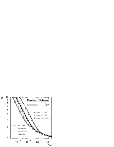
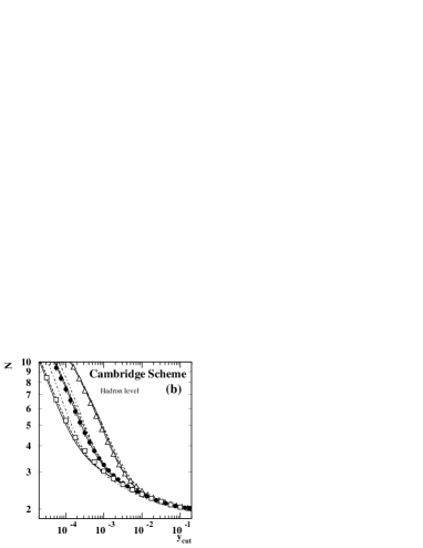
Figure 5: The mean jet multiplicities as obtained by the Durham (a) and Cambridge schemes (b) are plotted versus $y_{cut}$ at 35, 91 and 189 GeV. Data and Monte Carlo predictions are presented in the same form as in the previous figures.

Another relevant quantity in the context of QCD tests is the mean jet multiplicity $N$ defined by

$$N\equiv\frac{1}{\sigma}\sum_{n}n\sigma_{n},$$ (3)

for which various theoretical calculations exist. Measurements of $N$ versus $y_{cut}$ are presented for the Durham and Cambridge schemes in Fig. 5. The most complete theoretical predictions for this observable exist for these two schemes (cf. Appendix B.1.2).

The decrease of the average number of jets at given $y_{cut}$ with rising c.m.s. energy, as predicted by the energy-dependence of the strong coupling, is clearly visible. Differences between the Durham and Cambridge results are predicted by all Monte Carlo programs and confirmed by the data. At and above $\sqrt{s}=133$ GeV, the Durham scheme resolves systematically more jets than the Cambridge scheme.

All Monte Carlo predictions except that of COJETS are almost identical and lie within the error bars of the measurements. The COJETS prediction overshoots the data at $\sqrt{s}=91$ GeV and higher energies in regions of low $y_{cut}$, i.e. in regions of large jet multiplicities, consistent with the explanation suggested in the previous section and with OPAL results from the analysis of charged particle based quantities [10, 11].

4.2.4 Mean values of $y_{n}$

                                                                     

Figure 6: The average of the observables $y_{n}$ is plotted versus the c.m.s. energy $\sqrt{s}$ for the JADE (left) and Durham schemes (right). Data points are the measurements by the JADE and OPAL experiments. The error bars represent the total errors. Small horizontal lines indicate the size of the statistical errors. The curves are spline functions connecting the Monte Carlo predictions at the single c.m.s. energies.

Finally, we consider the mean values of the $y_{n}$ distributions given by

$$\langle y_{n}\rangle\equiv\frac{1}{\sigma}\int y_{n}\frac{\mbox{d}\sigma}{\mbox{d}y_{n}}\mbox{d}y_{n}$$ (4)

Measurements for $n=2$ through 5 for the JADE and Durham schemes are plotted in Fig. 6, against the c.m.s. energy. Hadron level predictions of PYTHIA, HERWIG, ARIADNE and COJETS at each of the eight c.m.s. energies are also shown. To facilitate qualitative comparisons, the respective predicted values at each c.m.s. energy are connected by spline functions to guide the eye. All generators are found in almost equal agreement with the data, except for COJETS.

Higher moments of the observables $y_{n}$ have also been investigated. They have large uncertainties and are not presented.

4.2.5 Summary

The measurements of jet-multiplicity related observables show scaling violations. PYTHIA, HERWIG and ARIADNE describe the data well, but COJETS predicts too many jets at and above $\sqrt{s}=91$ GeV.

5 Tests of Quantum Chromodynamics

5.1 Procedure for $\alpha_{s}$ Determinations

5.1.1 General Description

All jet-multiplicity based quantities considered in this analysis can be expressed as a power series in the strong coupling strength $\alpha_{s}$, where the coefficients of the powers of $\alpha_{s}$ depend on the observable. The approximate methods used here for the calculation of such series, pure ${\cal O}(\alpha_{s}^{2})$ predictions and matched ${\cal O}(\alpha_{s}^{2})$ and next-to-leading logarithmic predictions, are given in Appendix B. The coupling $\alpha_{s}$ will be regarded as unknown quantity, and the tests of perturbative QCD will consist of $\chi^{2}$ fits of the predictions to the measurements over ranges in $y_{cut}$ with $\alpha_{s}$ being fitted. These result in a determination of $\alpha_{s}$ at each c.m.s. energy.

All fits are performed at the hadron level, using only the statistical errors for the calculation of $\chi^{2}$. The error returned by the fit, i.e. the amount by which the fitted parameters may be varied without increasing $\chi^{2}$ by more than 1, defines the statistical errors of the fit results. Statistical correlations between bins in $y_{cut}$ are taken into account in the definition of $\chi^{2}$. At c.m.s. energies where the statistics are sufficient (i.e. $\sqrt{s}$=35 GeV, 44 GeV and 91 GeV) we determine the correlation matrix by subdividing the data sample, and the corresponding Monte Carlo sample used for the correction from detector to hadron level (see section 4.1.2), into $N$ independent subsamples and carrying out the entire analysis for each subsample. We choose $N=30$ at $\sqrt{s}=35$ GeV, $N=15$ at $\sqrt{s}=44$ GeV and $N=80$ at $\sqrt{s}=91$ GeV. At the higher c.m.s. energies we determine the correlations from Monte Carlo subsamples. At $\sqrt{s}=133$, 161 and 172 GeV, 30 subsamples are used. At the two higher c.m.s. energies, we use 50 subsamples each.

For the fits, we use only those observables for which there exist matched predictions of ${\cal O}(\alpha_{s}^{2})$ and NLLA calculations, i.e. the 2-jet fractions and the mean jet multiplicities as measured using the Durham and Cambridge schemes (see Appendix B). Fits are performed to the differential 2-jet fraction $D_{2}$ rather than the 2-jet fraction itself. Throughout the remainder of this chapter, the fitted variables shall be denoted $D_{2}^{D}$, $D_{2}^{C}$, $N^{D}$ and $N^{C}$ where upper indices $D$ and $C$ stand for the “Durham” and “Cambridge” scheme. One aim of the analysis is a comparison between the different types of calculations. The functional expressions to be used in the fits are given for the various matching schemes in (15), (16), (B.1.2) and (18) of Appendix B. Furthermore, fits of the pure ${\cal O}(\alpha_{s}^{2})$ predictions are carried out using (5) and (6). The parameter to be varied is always $\alpha_{s}$ as appearing in the equations. The renormalization scale factor $x_{\mu}\equiv\mu/\sqrt{s}$ is either kept fixed at $x_{\mu}=1$ or fitted simultaneously. Since the matched predictions are more complete than pure second-order calculations, one may expect an increased need for an adapted scale for the latter.

5.1.2 Hadronization Effects

In order to study the influence of hadronization on the quantities to be considered, we compare the predictions of PYTHIA 5.722, HERWIG 5.9 and ARIADNE 4.08 before and after the hadronization step. Each generator represents a different model for either hadronization or the partonic state. The generated event samples are the same as the ones used for the hadron level curves in Sect. 4.2. The COJETS generator which uses independent fragmentation is not considered since it was seen to describe the data badly in certain kinematic regions.

By the “parton level prediction,” we understand quantities determined from the set of particles emerging at the end of the parton shower generation, i.e. immediately before the hadronization step, including possible final state photon radiation. The curves in the lower partitions in Figs. 7, 8 and 9 are the ratios $f$ of the parton level over the hadron level predictions for the differential 2-jet fractions and the mean jet multiplicities as a function of $y_{cut}$ at all c.m.s. energies and for the three generators. The correction factors for PYTHIA, HERWIG and ARIADNE are shown, respectively, as solid, dashed and dotted lines. As is expected, hadronization corrections become notably smaller with rising c.m.s. energy.

We transform the theoretical calculations to hadron level by dividing the calculation for each value of $y_{cut}$ by the factors $f$ shown in the figures. The result is then compared with the hadron level measurement at the given $y_{cut}$. The PYTHIA generator will be used for the quoted central results.

5.1.3 Determination of Fit Ranges

The ranges of $y_{cut}$ for the fits have to be chosen with care. A fundamental limitation is given by the kinematic region over which the respective theoretical predictions can be assumed to be valid. In particular, for pure ${\cal O}(\alpha_{s}^{2})$ fits, the choice of the fit range is limited to large $y_{cut}$ regions. In the fits presented below, the fit range was adjusted separately for each type of calculation used.

In order to be as independent as possible of assumptions on the hadronization process, we require hadronization corrections to be less than 10% in the case of the differential 2-jet rates and less than 5% in the case of the mean jet multiplicity and to be insensitive to changes in hadronization parameters and models. As can be seen from Figs. 7 to 9, these conditions have to be loosened at lower energies and for observables obtained with the Cambridge jet finder, in order to make $\alpha_{s}$ determinations possible at all. The condition of small hadronization corrections turns out to be the most stringent limitation of the fit ranges at low c.m.s. energies. The size of the corrections for experimental effects is also taken into account, but not considered as crucial because the simulation of the detectors is believed to be rather reliable and, in most cases, these corrections are clearly smaller than those for hadronization.

As a further limitation we demand that the value of $\chi^{2}/d.o.f.$ obtained in the fit be not dominated by the contribution from a single bin at the boundary of the fit range. Another necessary check concerns the stability of the fit results under variations of the fit range. The results can only be regarded as reliable if they do not change significantly when the boundaries of the fit range are varied around the chosen values.

Observing all conditions listed, we try to maximize the fit range in order to give the most significant possible results.

5.1.4 Determination of Systematic Errors

The determination of $\alpha_{s}$ is repeated with variations in the details of the analysis procedure. For each variation, the absolute difference between the obtained value for $\alpha_{s}$ and the central value is taken as the systematic error from the respective source. All contributions are added quadratically.

At all energies, the same systematic variations of the selection procedure are performed as in the measurements of the jet quantities themselves (see Sect. 4.1.3), and the fit is repeated using only charged tracks. At the c.m.s. energies of 35 GeV, 44 GeV, 91 GeV and 189 GeV, one observes in some cases a significant dependence of the resulting $\alpha_{s}$ value on the choice of the fit range. In order to estimate this uncertainty, both the upper and the lower boundaries of the fit ranges are varied by one bin in both directions, keeping the respective opposite boundary fixed. All contributions mentioned, added in quadrature, define the total experimental systematic error.

Uncertainties from the hadronization models used for the transformation of the QCD prediction to hadron level are determined by varying the parameters and the Monte Carlo generators used. In particular, the parameter $b$ appearing in the Lund fragmentation function, used for the hadronization of u, d and s quarks by the PYTHIA generator, and the width $\sigma_{q}$ of the transverse momentum distribution of the produced hadrons with respect to the parent parton are each varied in both directions within the uncertainties allowed by the OPAL tunes [21]. At $\sqrt{s}=133$ GeV and below, the parameter $Q_{0}$ defining the end of the parton shower cascade is also varied within its uncertainties around the central value of 1.9 GeV to 1.4 GeV and 2.4 GeV, yielding, on the average, correspondingly smaller and higher numbers of partons at the end of the cascade. At the higher c.m.s. energies, these variations are replaced by a more radical change to $Q_{0}=4$ GeV, and the fits are repeated using HERWIG 5.9 and ARIADNE 4.08 as described in Sect. 5.1.2 instead of PYTHIA.

All theoretical predictions to be used make the assumption of zero quark masses. In an attempt to estimate the effect of this, we repeat the fit using a Monte Carlo sample containing only light primary quarks (u, d, s and c) for the transformation to hadron level. The quadratic sum of all contributions listed defines the overall hadronization uncertainty of the result.

Finally, the uncertainty in the choice of the renormalization scale must be accounted for. In the fits where the scale factor $x_{\mu}$ is kept fixed at 1 for the central results, the fit is repeated with $x_{\mu}=0.5$ and $x_{\mu}=2$. Usually, the choice of a smaller scale will entail a decrease of the fitted $\alpha_{s}$, while a larger scale will give larger values of $\alpha_{s}$. The different deviations obtained from varying $x_{\mu}$ in both directions are then added asymmetrically to the hadronization error to yield the total error from theory. In cases where both variations of $x_{\mu}$ let $\alpha_{s}$ change in the same direction, the average of both deviations is taken and added as symmetric error.

5.2 QCD Tests at Fixed c.m.s. Energies

5.2.1 Fit Results

35 GeV

                                                    

                                                    

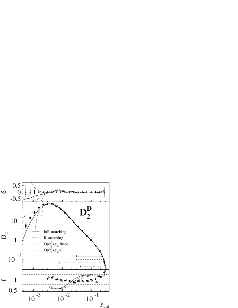
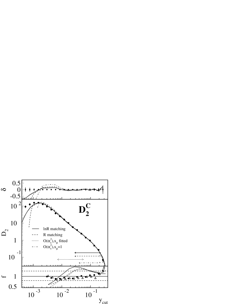
Figure 7: The central parts of the plots display the results of fits of various theoretical predictions (smooth curves) in comparison with hadron level measurements (data points) of the four observables $D_{2}^{D}$, $D_{2}^{C}$, $N^{D}$ and $N^{C}$ at $\sqrt{s}=35$ GeV. The error bars on the data represent the total errors, the small horizontal lines the pure statistical errors which were used in the fits. Horizontal arrows indicate the respective fit ranges. The normalized difference between predictions and the data, $\delta$, is shown above each plot. The small sections below each plot indicate the correction factors $f$ for experimental and hadronization effects. The hadronization corrections are shown as lines and shaded bands as described in the text. The experimental corrections are represented as open triangles and filled circles, respectively, for the 1982 and 1986 runs.

91 GeV

                                                    

                                                    

Figure 8: The fit results at $\sqrt{s}=$91 GeV are shown in the same form as in Fig. 7.

189 GeV

                                                    

                                                    

Figure 9: The fit results at $\sqrt{s}=$189 GeV are shown in the same form as in Fig. 7. At this energy, the statistical fluctuations of the data points are too large to draw any meaningful conclusions from the normalized differences between the predictions and the measurement for $D_{2}^{D}$ and $D_{2}^{C}$. They are therefore not shown in the plot.

Fits of the different matched calculations described in Appendix B.1.2, i.e. the $\ln R$ matching, the $R$ matching and their modified variants, as well as ${\cal O}(\alpha_{s}^{2})$ predictions have been performed for the measured observables $D_{2}^{D}$, $D_{2}^{C}$, $N^{D}$ and $N^{C}$. In the case of the ${\cal O}(\alpha_{s}^{2})$ calculations, fits both with a fixed QCD scale factor of 1 and with a variable scale $x_{\mu}$ were tried. The fitted predictions of the various matching schemes and the ${\cal O}(\alpha_{s}^{2})$ calculations for $\sqrt{s}=35$ GeV, 91 GeV and 189 GeV are shown in the central parts of Figs. 7, 8 and 9 as smooth lines. Similar fits were done at all energies. At $\sqrt{s}=35$ GeV, no stable fits with a fitted QCD scale could be obtained for observables $N^{D}$ and $N^{C}$. The small sections below each plot give the correction factors $f$ for experimental and hadronization effects. In the additional small section above the plots, the differences between the fitted predictions and the data, denoted as $\delta$, is plotted, normalized to the measured value. The relative total and statistical errors on the data are shown along the $\delta=0$ line.

The fitted values for $\alpha_{s}$ are summarized in Figs. 10 and 11 with their total errors (outer bars) and purely experimental errors (inner bars). The $\chi^{2}/d.o.f.$ is given for each result to the right of the plots. For all observables the same systematic pattern of the results from each calculation type used repeats at all c.m.s. energies. Furthermore, the theoretical uncertainties in the predictions resulting from the choice of the calculation type are at least as large as the experimental errors, in particular at $\sqrt{s}=35$ GeV, 91 GeV, 183 GeV and 189 GeV. Further refinements of the experimental procedure and increase of statistics will therefore not lead to significantly more precise results for $\alpha_{s}$ as long as theoretical uncertainties can not be reduced.

Fits of ${\cal O}(\alpha_{s}^{2})$ calculations with a fixed QCD scale of 1 require a limitation of the fit range to regions of large $y_{cut}$ in order to achieve acceptable values of $\chi^{2}/d.o.f.$ The resulting statistical errors are correspondingly large. As can be seen from Fig. 10, the results for $\alpha_{s}$ are generally high at lower c.m.s. energies, while, at $\sqrt{s}\geq 133$ GeV, they are similar to those obtained with the $\ln R$ and modified $R$-matchings.

Allowing the scale factor $x_{\mu}$ to vary allows the fit range to be extended to lower $y_{cut}$. In fact, a wider fit range is required in most cases to obtain stability of the fits. At the lower c.m.s. energies of 35 GeV and 44 GeV, the fit ranges have to be extended into regions where hadronization uncertainties become large, resulting in comparatively large theoretical errors of the results.

In the case of the Durham scheme, the fitted $\alpha_{s}$ values obtained using ${\cal O}(\alpha_{s}^{2})$ predictions with a fitted scale are systematically smaller than the results from fits with a constant $x_{\mu}$. In contrast, in the case of the Cambridge scheme they are somewhat larger. We conclude that a suitable choice of $x_{\mu}$ is able to improve the agreement of the predictions with the measurements.

         $D_{2}^{D}$                                                        $D_{2}^{C}$

                                                                      $\chi^{2}/d.o.f.$                                                  $\chi^{2}/d.o.f.$

                                               

Figure 10: Fitted $\alpha_{s}$ values obtained using the different theoretical predictions described in the text for variable $D_{2}^{D}$ and $D_{2}^{C}$ with the respective experimental (inner) and total (outer) errors. The $\chi^{2}/d.o.f.$ values of each fit are given in the rightmost column.

         $N^{D}$                                                        $N^{C}$

                                                                      $\chi^{2}/d.o.f.$                                                  $\chi^{2}/d.o.f.$

                                               

Figure 11: Fitted $\alpha_{s}$ values obtained using the different theoretical predictions described in the text for variable $N^{D}$ and $N^{C}$, presented as in Fig. 10. At $\sqrt{s}=$35 GeV, no stable fits could be obtained using pure ${\cal O}(\alpha_{s}^{2})$ calculations with a free QCD scale factor.

a) Fit results for the 2-jet fractions
The comparison of the quality of the fits (i.e. the $\chi^{2}/d.o.f.$) does not indicate a clear preference for one of the matching schemes for either one of the variables. The normalized deviations $\delta$ also behave similarly for all matching schemes. Only in the case of the Cambridge scheme at $\sqrt{s}=$91 GeV, they differ somewhat because rather distinct fit ranges had to be chosen for the different schemes.

The results obtained with the $\ln R$ and the modified $\ln R$-matching with $y_{max}=1/3$ turn out to be virtually identical up to at least the third decimal place of the extracted value for $\alpha_{s}$, which is in accordance with the findings of a previous OPAL analysis [34]. The fit results are therefore not shown separately, but only for the $\ln R$-matching. The results of the modified $R$-matching are also generally similar to those of the $\ln R$-matching, but have slightly larger theoretical errors. $R$-matching, however, leads to systematically low values of $\alpha_{s}$ for both jet algorithms. In fact, the $R$-matching results are in most cases the lowest of all calculation types under consideration. As is explained in Appendix B.1.2, the $R$-matching may be expected to describe the data less well than the modified variant because the term $G_{21}L$ is not exponentiated. The observed behaviour seems to indicate that the inclusion of this term has more significance than the choice between $\ln R$ and $R$-matching. We decide to follow the practise of [34] and use the $\ln R$-matching for the final results. The difference plots $\delta$ also indicate that the $\ln R$ matching provides a good description of the data over a wider range in $y_{cut}$ than both the $R$ matching and ${\cal O}(\alpha_{s}^{2})$ calculations.

The stability of the $\ln R$-matching fits under variations of the fit range boundaries turns out to be generally good.

b) Fit results for the mean jet multiplicities
The fits of ${\cal O}(\alpha_{s}^{2})$ predictions for $N^{D}$ and $N^{C}$ with the QCD scale factor fixed at $x_{\mu}=1$ describe the data significantly less well in the regions of low $y_{cut}$ than all the other fits, requiring a corresponding limitation of the fit ranges. Allowing $x_{\mu}$ to vary results in an improved agreement between data and predictions. Only at $\sqrt{s}=35$ GeV, the ${\cal O}(\alpha_{s}^{2})$ calculations with $x_{\mu}=1$ seem to follow the data well even in low $y_{cut}$ regions. A closer inspection reveals, however, that the agreement at higher $y_{cut}$, i.e. within the selected fit range, is worse.

The necessity of keeping hadronization uncertainties small limits the fit ranges rather strongly and leads to somewhat larger statistical errors than in the case of the 2-jet rates. Fig. 11 shows that fits with a free QCD scale always result in values of $\alpha_{s}$ which are smaller than those from any other fits, while those with $x_{\mu}$ fixed to 1 yield usually the largest values.

The agreement between data and theory, according to the normalized differences $\delta$, is again rather similar for all matching schemes. All types of predictions display the property of overshooting the data below some $y_{cut}$, i.e. predicting too many jets.

For both jet algorithms, the fit results for $\alpha_{s}$ turn out to be less dependent on the choice of the matching scheme than is the case for the 2-jet rates, and the corresponding uncertainties are currently much smaller than the experimental errors. The modified $\ln R$-matching of the Durham scheme contains the additional term $LH_{21}$ in the exponent (see Appendix B.1.2) and should therefore be a better description of the measurements than the $\ln R$-matching. As can be seen from Fig. 11, the results obtained by the modified $\ln R$-matching, the $R$-matching and the $\ln R$-matching are always quite similar. Considering the small dependence on the calculation type mentioned above, one could expect to obtain rather precise determinations of $\alpha_{s}$ from these variables if better hadronization models were available which would allow to extend the fit range towards lower $y_{cut}$.

The mean jet multiplicities exhibit a stronger dependence on the choice of the boundaries of the fit ranges than the 2-jet rates, in particular at small c.m.s. energies. The fit range dependence (and therefore also the corresponding systematic error) is larger for the $R$-matching and the modified $\ln{R}$-matching than for $\ln{R}$-matching. We conclude that the latter is a more appropriate description, valid over a wider range in $y_{cut}$, and decide to use it for the main quoted fit results.

5.2.2 Investigation of the renormalization scale dependence

$D_{2}^{D}$                                                              $N^{D}$

                                                                                                               

                                                                                                               

                                                                                                               

Figure 12: Sensitivity of fit results to the scale $x_{\mu}$. The solid and dashed lines are, respectively, the fitted $\alpha_{s}$ and the corresponding $\chi^{2}/d.o.f.$ as a function of the QCD scale $x_{\mu}$ for observables $D_{2}^{D}$ (left) and $N^{D}$ (right). Filled and empty squares denote $\alpha_{s}$ and $\chi^{2}/d.o.f.$ for a fitted scale; circles have the same meaning for a fixed scale of 1. For $D_{2}^{D}$ at $\sqrt{s}=189$ and $N^{D}$ at 35 GeV, results are presented only for the $\ln{R}$-matching scheme. In all other cases, fits of the pure ${\cal O}(\alpha_{s}^{2})$ predictions are also presented in the lower partitions of the plots.

The fits of the ${\cal O}(\alpha_{s}^{2})$ calculations show clearly that the data are better described by fixed order QCD predictions if small renormalization scales are used, with $x_{\mu}$ typically between 0.15 and 0.2 in the case of the 2-jet fractions and between 0.03 and 0.1 in the case of the mean jet multiplicities. Similar results have been obtained in many other analyses involving event shape variables (e.g. [6, 34, 35]). The value of the best scale depends strongly on the observable. Although the fitted value of $x_{\mu}$ does not bear any physical significance, its deviation from unity indicates the importance of neglected higher order contributions in the fixed order calculation for the given observable.

The inclusion of higher order terms in the matched predictions leads one to expect that the dependence of these predictions on the QCD scale factor $x_{\mu}$ will be reduced, as compared with the ${\cal O}(\alpha_{s}^{2})$ calculations. This has, in fact, been confirmed in [6, 34]. As was done in those publications, we have studied the $x_{\mu}$ dependence of the fit results by performing fits for $\alpha_{s}$ at various fixed values of $x_{\mu}$. Examples of the results for $D_{2}^{D}$ and $N^{D}$ are shown in Fig. 12 at $\sqrt{s}=35$, 91 and 189 GeV. The solid lines demonstrate the behaviour of $\alpha_{s}$ as a function of $x_{\mu}$ for both matched and ${\cal O}(\alpha_{s}^{2})$ predictions. The fit ranges used for the matched predictions are the same as for the central values of $\alpha_{s}$ from the previous section. In the case of the ${\cal O}(\alpha_{s}^{2})$ predictions, the fit ranges from the simultaneous fits for $\alpha_{s}$ and $x_{\mu}$ are taken. The shape of the curves depends rather strongly on the fit range, which is why the circular and square markers are sometimes not situated on the corresponding curves. In general, an extension of the fit range causes the minima of the $\chi^{2}$ curves to become more pronounced, though the positions in $x_{\mu}$ of the minima are found to be mostly unaffected by such changes.

At 189 GeV statistics are low, and the fits of the ${\cal O}(\alpha_{s}^{2})$ predictions tend to become unstable under variations of the QCD scale for larger $x_{\mu}$. The corresponding curves are therefore not shown. Stability of the fits requires the limitation of the fit ranges to those used in the previous section for fits with fixed scales. Instabilities are further encountered at $\sqrt{s}=35$ GeV in the case of the matched predictions of the 2-jet fractions at low $x_{\mu}$, as well as for the two-parameter fits of the ${\cal O}(\alpha_{s}^{2})$ calculations for the mean jet multiplicities.

As can be seen in Fig. 12, the dependence of $\alpha_{s}$ on the scale in the vicinity of $x_{\mu}=1$ is generally much smaller with $\ln R$-matching than with ${\cal O}(\alpha_{s}^{2})$ calculations. Furthermore, fits of the matched predictions with a free QCD scale result in very shallow minima in $\chi^{2}$ and correspondingly large errors in the fitted parameters. Sometimes they do not converge at all. In some cases, convergence can be achieved by sufficiently extending the fit range towards low $y_{cut}$. The results for $x_{\mu}$ are then usually found to be closer to 1. We conclude that the matched predictions indeed show little preference for any specific choice of the QCD scale, while the second-order calculations require rather definite values of $x_{\mu}$ to describe the data well. However, as can be seen in the figures, the $x_{\mu}$ dependence of the resulting $\alpha_{s}$ is still sizeable.

                                                                              

Figure 13: The combined results for $\alpha_{s}(Q)$ ($Q=\sqrt{s}$) from fits of the matched predictions plotted versus the c.m.s. energy. Arranged around the combined values are the contributing separate results for each of the four observables under consideration. All results are shown with their total errors (outer error bars) and the purely experimental (inner bars) component of the errors. A three-loop evolution of the current world average [36] is overlaid as solid and dotted lines.

5.2.3 Systematic Errors of the Main Result

Based on the investigations carried out in the previous sections, we use the $\ln{R}$-matching scheme for our final results for all observables. Tables 9 through 11 in Appendix C list the final results for $\alpha_{s}$ for all variables and c.m.s. energies, along with the composition of their errors. We discuss the systematic errors for this scheme.

At all c.m.s. energies, the use of only charged tracks rather than both tracks and electromagnetic clusters has a large effect on the result. At JADE energies, variations of the selections generally contribute little to the systematic errors. At c.m.s. energies of 133 GeV and above, however, the influence of variations in the selections becomes sizeable. This is to be expected since the selections themselves play a more important role here than at the lower energies. The restriction of the cut on the thrust axis, which is applied at all c.m.s. energies, induces mostly small effects.

The hadronization errors of the results are, in particular at lower c.m.s. energies, dominated by differences between the generators (i.e. HERWIG or ARIADNE). This could be anticipated considering the size of the hadronization corrections shown in Figs. 7 to 9. A similar behaviour is seen for the dependence of the results on $x_{\mu}$ which is largest at low c.m.s. energies. The influence of the omission of b quarks in the hadronization model and of varying the termination point of the parton shower is sizeable and relatively independent of the c.m.s. energy. Variations of the hadronization parameters $b$ and $\sigma_{q}$ have very small effects throughout.

5.2.4 Combination of the Fit Results

We combine the results obtained using the four observables, separately at each c.m.s. energy by forming the mean value, taking into account the covariance matrix corresponding to the total errors of the individual values. The statistical correlations are determined from the data/Monte Carlo subsamples of Sect. 5.1.1. The systematic uncertainties are treated as fully correlated, aside from the variations of $x_{\mu}$ and those of the bin boundaries which are considered as uncorrelated and added to the diagonal of the matrix only. To this end, the scale uncertainties are made symmetric by taking the mean value of the two separate deviations. In order to break up the total error into its single components, the mean is determined using, respectively, the covariance matrix corresponding to only statistical, only experimental, and only experimental and hadronization uncertainties. Fig. 13 gives an overview of the combined results, as well as the results from each single observable with their experimental and total errors. The combined results are given in Table 4. The values listed in the right column of the table are three-loop evolutions to $\sqrt{s}=M_{Z^{0}}$. The results are compatible within their errors.

$\sqrt{s}$	$\alpha_{s}(\sqrt{s})$					$\alpha_{s}(M_{Z^{0}})$
[GeV]		(stat.)	(exp. sy.)	(hadron.)	(scale)		(stat.)	(exp. sy.)	(hadron.)	(scale)
35	0.1445 $\pm$	0.0007 $\pm$	0.0029 $\pm$	0.0042 $\pm$	0.0033	0.1226 $\pm$	0.0005 $\pm$	0.0021 $\pm$	0.0030 $\pm$	0.0024
44	0.1287 $\pm$	0.0010 $\pm$	0.0044 $\pm$	0.0039 $\pm$	0.0012	0.1149 $\pm$	0.0008 $\pm$	0.0035 $\pm$	0.0031 $\pm$	0.0009
91	0.1179 $\pm$	0.0001 $\pm$	0.0016 $\pm$	0.0038 $\pm$	0.0021	0.1179 $\pm$	0.0001 $\pm$	0.0016 $\pm$	0.0038 $\pm$	0.0021
133	0.1080 $\pm$	0.0019 $\pm$	0.0054 $\pm$	0.0014 $\pm$	0.0010	0.1139 $\pm$	0.0021 $\pm$	0.0061 $\pm$	0.0016 $\pm$	0.0011
161	0.1040 $\pm$	0.0020 $\pm$	0.0030 $\pm$	0.0019 $\pm$	0.0012	0.1125 $\pm$	0.0023 $\pm$	0.0035 $\pm$	0.0022 $\pm$	0.0014
172	0.1084 $\pm$	0.0037 $\pm$	0.0025 $\pm$	0.0016 $\pm$	0.0024	0.1188 $\pm$	0.0045 $\pm$	0.0031 $\pm$	0.0020 $\pm$	0.0030
183	0.1079 $\pm$	0.0020 $\pm$	0.0024 $\pm$	0.0020 $\pm$	0.0011	0.1193 $\pm$	0.0024 $\pm$	0.0029 $\pm$	0.0024 $\pm$	0.0013
189	0.1081 $\pm$	0.0012 $\pm$	0.0019 $\pm$	0.0021 $\pm$	0.0007	0.1201 $\pm$	0.0015 $\pm$	0.0023 $\pm$	0.0026 $\pm$	0.0008

Table 4: Combined results from fits of matched predictions, along with the statistical, experimental systematic, hadronization and QCD scale errors (left column). The values in the right column are results of a three-loop evolution of each result to $Q=M_{Z^{0}}$.

As can be seen in the Fig. 13, the separate results are distributed in roughly the same pattern at each c.m.s. energy. The solid and dotted lines represent a three-loop evolution of the current world average of $\alpha_{s}(M_{Z^{0}})=0.119\pm 0.004$ [36] with its total error. No significant discrepancies between the curve and any of the fit results can be noted. Our values agree with the world average within their experimental errors. Our results using the 2-jet fraction of the Durham scheme are also in good agreement with previous determinations using resummed calculations at these energies (see, e.g., [6, 10, 11, 34, 37, 38]).

The difference $\Delta\alpha_{s}\equiv\alpha_{s}(Q)-\alpha_{s}(M_{Z^{0}})$ is plotted in Fig. 14. Again, the inner error bars in the plot represent the total experimental errors while the outer bars include also hadronization and QCD scale uncertainties. The statistical and experimental systematic errors are obtained from those quoted in Table 4 assuming that correlations between different energies can be neglected. In order to take correlations of the theoretical errors into account, each difference $\Delta\alpha_{s}$ was calculated separately under each variation of the hadronization model and of the QCD scale. As usual, the difference between the value of $\Delta\alpha_{s}$ obtained after each such variation and its central value was counted as a contribution to the systematic error. The contributions to the hadronization error were combined in quadrature.

Finally, in order to obtain a single result for $\alpha_{s}$, we perform a fit of the three-loop running of $\alpha_{s}$ to the values of Fig. 13, the fitted variable being $\alpha_{s}(M_{Z^{0}})$. We assume that correlations between the total experimental errors can be neglected and use these for the determination of $\chi^{2}$. The resulting fit error is taken as the total experimental error of the final result. The statistical component is assessed by repeating the fit using only statistical errors. The total hadronization and scale errors are then calculated as for $\Delta\alpha_{s}$, i.e. by repeating the fits under each variation. The final result of 0.1187$\stackrel{{\scriptstyle\textstyle\mbox{\scriptsize+0.0034}}}{{\mbox{\scriptsize$-$0.0019}}}$ is given with its individual error contributions and the value of $\chi^{2}/d.o.f.$ in Table 5.

Figure 14: The difference $\Delta\alpha_{s}\equiv\alpha_{s}(Q)-\alpha_{s}(M_{Z^{0}})$ versus $Q=\sqrt{s}$ from $\alpha_{s}$ fits of matched predictions. The definition of the error bars is as in Fig. 13. The solid line represents the current world average.

$\alpha_{s}(M_{Z^{0}})$	0.1187
$\chi^{2}/d.o.f.$	7.85/7
Stat. error	$\pm 0.0001$
Total exp.	$\pm 0.0010$
$b+1\sigma$	$-0.0001$
$b-1\sigma$	$+0.0002$
$\sigma_{q}+1\sigma$	$+0.0001$
$\sigma_{q}-1\sigma$	$<0.0001$
$Q_{0}=2.4$ GeV	$+0.0007$
$Q_{0}=1.4$ GeV	$-0.0004$
udsc only	$+0.0010$
HERWIG	$-0.0010$
ARIADNE	$-0.0002$
Total hadronization	$\pm 0.0016$
$x_{\mu}=0.5$	$-0.0001$
$x_{\mu}=2$	$+0.0028$
	+0.0034
Total error	-0.0019

Table 5: The result for $\alpha_{s}(M_{Z^{0}})$ obtained from a fit of the three-loop running of the strong coupling to the combined values determined using matched QCD calculations at single c.m.s. energies (Table 4), with the individual error contributions. For each systematic variation of Monte Carlo parameters and of the QCD scale, the deviation with respect to the central value is given with a sign indicating the direction of the deviation.

5.3 $\alpha_{s}(M_{Z^{0}})$ from the Energy Evolution of Jet Observables

The availability of measurements performed over a wide range of c.m.s. energy with very similar experimental conditions suggests investigations of the c.m.s. energy dependence of jet-related observables rather than analyses at fixed energies. In Sect. 4, the energy evolution of jet fractions was already qualitatively observed, and the extracted $\alpha_{s}$ values shown in Fig. 13 were seen to be in accordance with the QCD prediction of the running of the strong coupling.

Similar analyses have been done based on data from many ${\rm e}^{+}{\rm e}^{-}$ collision experiments, present and past. For an early test of the running of $\alpha_{s}$, the three-jet fraction was used (e.g. [8]). This is, in lowest order, simply proportional to $\alpha_{s}$. The JADE scheme was employed for these analyses because it has the smallest and least energy-dependent hadronization corrections of all clustering schemes at low c.m.s. energies. More recent measurements have been mainly concerned with the measurements of the energy evolution of event shape moments and of the mean jet multiplicity (e.g. [6, 14, 37, 39]).

In this analysis, the energy evolution of the three-jet fraction $R_{3}$ at a fixed value of $y_{cut}$ and that of the mean values of the observable $y_{2}$ are compared with the predictions of QCD for various clustering algorithms.

5.3.1 Analysis Procedure

Figure 15: Mean values of $y_{2}$ as obtained with the JADE and Durham schemes at parton level versus the c.m.s. energy $\sqrt{s}$. The solid lines represent the fitted ${\cal O}(\alpha_{s}^{2})$ predictions at a fixed QCD scale of 1.

The comparisons between measurement and predictions are done by making $\chi^{2}$ fits to the respective observables over the entire range of c.m.s. energies considered in our analysis, taking $\alpha_{s}(M_{Z^{0}})$ as the fitted variable. The expressions for the ${\cal O}(\alpha_{s})$ and ${\cal O}(\alpha_{s}^{2})$ coefficients in the prediction are taken from [40] for the JADE scheme and from [29] for the Durham and Cambridge schemes. The expression to be fitted to the mean value of $y_{2}$ is given by (7) of Appendix B. The coefficients $A$ and $B$ were obtained from runs of the EVENT2 program [41, 42].

In the case of the fits to the three-jet fractions, a specific value of $y_{cut}$ has to be selected at which the jet fraction is given. Here, we select a value in a region where the sensitivity to changes in the c.m.s. energy is large (see Figs. 1, 2 and 3) and hadronization corrections are small. In the case of the JADE scheme, the value of $y_{cut}=0.08$ from [43] is used. For the Durham and Cambridge schemes, we take $y_{cut}=0.01$.

For the moments of some event shape variables, there exist non-perturbative corrections (also called “power corrections”) to the perturbative calculations [44]. It was found in [6] that corrections of order $1/Q$ as well as $1/Q^{2}$ to the mean values of $y_{2}$ as obtained with the Durham scheme can be neglected at the c.m.s. energies considered in this analysis. Hadronization corrections for the three-jet fractions at the chosen value of $y_{cut}$ are found to be small (between 2% and 11%) for the JADE and Durham schemes, but large (about 25%) for the Cambridge scheme at low c.m.s. energies. We perform the fits for all observables at parton level. The transformation of the measurements from hadron to parton level is done separately at each c.m.s. energy by means of multiplicative factors which are obtained from the same Monte Carlo samples as were used for the $\alpha_{s}$ fits. The factors predicted by the PYTHIA 5.722 Monte Carlo at standard OPAL tune are used to correct the results.

The systematic errors can not be treated by repeating the fits with purely statistical errors for each systematic variation, because the systematic variations applied are essentially different at each c.m.s. energy. We therefore use the total experimental errors of each measurement for the calculation of the $\chi^{2}$ and take the resulting fit error as the overall experimental error of $\alpha_{s}$. Its statistical component is determined by repeating the fit using only statistical errors. Hadronization uncertainties are determined by repeating the fits with variations of the Monte Carlo predictions for the correction factors from hadron to parton level. We apply only the variations leading to the predominant error contributions in the fits of the previous section, i.e. changes to HERWIG and ARIADNE and the removal of the b quark. The absolute differences from the central result are again added in quadrature to get the total hadronization error.

Fits are carried out both with a constant QCD scale factor, fixed at unity, and with $x_{\mu}$ taken as an additional fit parameter. In the first case, systematic variations of $x_{\mu}$ to 0.5 and 2 are performed and added asymmetrically to the hadronization error.

5.3.2 Results from the Energy Evolution Fits

         

         

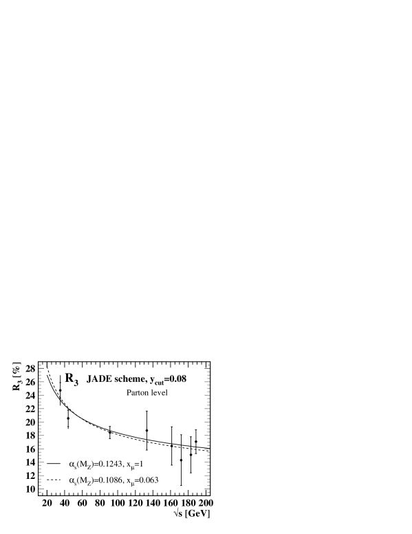
Figure 16: The 3-jet fraction as obtained with the JADE, Durham and Cambridge schemes at parton level versus the c.m.s. energy $\sqrt{s}$. The solid lines represent the fitted ${\cal O}(\alpha_{s}^{2})$ predictions at a fixed QCD scale of 1, the dashed lines are the results obtained with a fitted scale.

Fig. 15 shows the measurements of $\langle y_{2}\rangle$ for the JADE and the Durham scheme at parton level with the result of the fit at fixed $x_{\mu}$. The inner error bars denote the size of the purely experimental errors, the outer bars include also hadronization errors. The obtained values for $\alpha_{s}(M_{Z^{0}})$ from the fits shown are listed in Table 12 of Appendix C with the deviations induced by each systematic variation, as before. The total errors are of the same order of magnitude as from the fits at separate c.m.s. energies. Fits with a free QCD scale $x_{\mu}$ lead to errors of almost 100% in the scale for both observables. We therefore present the results obtained at a fixed scale of 1, performing the usual variations to estimate the error from the scale uncertainty. The somewhat small values of $\chi^{2}/d.o.f.$ indicate correlations in the systematic uncertainties.

The results of the fits to the three-jet fractions are summarized in Table 13 of Appendix C and are displayed in Fig. 16. Unlike the previous fits to the mean values of $y_{2}$, the fits with a free QCD scale lead to smaller errors in $x_{\mu}$. The corresponding prediction is added as a dashed line in the plots. The optimized scales again turn out to be significantly smaller than $x_{\mu}=1$. The fit results for $\alpha_{s}$ with a fitted scale are systematically smaller than with a fixed scale of 1. In order to be able to estimate the error induced by scale uncertainties, we quote central results for $x_{\mu}=1$ and vary the scale to 0.5 and 2.

We combine the separate results with $x_{\mu}=1$ from the five observables into one value for $\alpha_{s}(M_{Z^{0}})$. The combined result is calculated by taking the average of the remaining five single values, weighted with their respective total errors. We assume total experimental errors to be largely unaffected by correlations and determine these also by taking the weighted mean of the single values. The error contributions from each hadronization and QCD scale variation are determined in the same way separately for each variation, resulting in the overall hadronization and asymmetric scale error of the combined value. Table 6 shows the combined result 0.1181$\stackrel{{\scriptstyle\textstyle\mbox{\scriptsize+0.0066}}}{{\mbox{\scriptsize$-$0.0056}}}$ with its single error components.

$\alpha_{s}(M_{Z^{0}})$	0.1181
Stat. error	$\pm 0.0006$
Total exp.	$\pm 0.0020$
udsc only	$+0.0015$
HERWIG	$-0.0035$
ARIADNE	$-0.0011$
Total hadronization	$\pm 0.0039$
$x_{\mu}=0.5$	$-0.0035$
$x_{\mu}=2$	$+0.0048$
	+0.0066
Total error	-0.0056

Table 6: The weighted mean of $\alpha_{s}(M_{Z^{0}})$ as determined from the energy evolution of observables $\langle y_{2}^{J}\rangle$, $\langle y_{2}^{D}\rangle$, $R_{3}^{J}$, $R_{3}^{D}$ and $R_{3}^{C}$, with the single error contributions. For each systematic variation of Monte Carlo parameters and of the QCD scale, the deviation with respect to the central value is given with a sign indicating the direction of the deviation.

5.4 MLLA Prediction for the Mean Jet Multiplicity

                                               

                                               

                                               

                                               

Figure 17: The mean jet multiplicity as obtained with the Durham scheme plotted versus parameter $y_{cut}$ at all energies. The MLLA prediction according to [45] for each energy is the solid line and the same prediction shifted by $Q_{0}^{2}/s$ in $y_{cut}$ as described in the text is the dashed line.

Lastly, we compare our measurements of the mean jet multiplicity of the Durham scheme with a recent hadron level prediction [45]. The calculation was carried out in the framework of the modified leading logarithmic approximation (MLLA) in the form of a cascade of successive parton branchings which is continued until the relative transverse momentum between the two partons emerging from the branching falls below a cut-off $Q_{0}$. Assuming “local parton-hadron duality” to be valid and setting $Q_{0}$ to a value of typical hadron masses, the prediction may be compared with hadron level measurements. The lower portions of each part of Fig. 17 show the hadron level measurement of $N^{D}$ at all c.m.s. energies with their errors as in Fig. 5 and the MLLA prediction [46] as a solid line. The cut-off $Q_{0}$ is fixed by $\ln{(Q_{0}/\Lambda_{QCD})}=0.015$ with $\Lambda_{QCD}=500$ MeV [45]. This value was obtained from fits to measured hadron multiplicities over a c.m.s. energy range from 1.5 GeV to 91 GeV. The smaller captions above each plot show the normalized difference $\delta$ between measurements and predictions, defined as in Sect. 5.2.1. A first observation is that the MLLA curves rise more rapidly than the data below some $y_{cut}$ as a result of the singularity in the strong coupling as the transverse parton momentum comes close to $\Lambda_{QCD}$. The difference seen at low values of $y_{cut}$ becomes smaller for higher c.m.s. energies.

The MLLA prediction assumes quarks to be massless. In order to artificially introduce a hadron mass in the calculation, it is suggested in [45] that one may compare the parton transverse momenta $k_{\perp}$ with the transverse energies of the hadrons given by $E_{\perp}=\sqrt{k_{\perp}^{2}+Q_{0}^{2}}$. In the application of the predictions to the Durham jet multiplicities, this amounts to comparing the measurement at some $y_{cut}$ with the prediction at $y_{cut}+Q_{0}^{2}/s$, i.e. a relative shift by a fixed amount along the $y_{cut}$ axis. The dashed lines in the plots represent the prediction after this shift. At $\sqrt{s}=35$ GeV and 44 GeV, the predictions somewhat undershoot the data after the shift, showing that such a crude method for introducing a hadron mass into the calculations works less well at such low energies.

At all c.m.s. energies, the data fall below the MLLA predictions in the region of medium $y_{cut}$. This behaviour is also observed in [45] for $\sqrt{s}=91$ GeV and is there attributed to the omission of higher loops in the definition of $\alpha_{s}$.

6 Summary

We have performed QCD related measurements at c.m.s. energies of 35, 44, 91.2, 133, 161, 172, 183 and 189 GeV using data from the JADE and OPAL experiments which are very similar in their components used in the analysis. The same measuring techniques were applied in the two experiments, including details of the selections and the method of reconstructing single particle four-momenta. The results of the measurements display the same systematic behaviour over the entire c.m.s. energy range, suggesting that the desired homogeneity of the analysis is indeed realized.

Hadron level measurements of $n$-jet fractions, differential jet fractions, distributions in the variables $y_{n}$ and mean jet multiplicities have been presented up to large jet multiplicities and down to very low values of $y_{cut}$ using the JADE, Durham and Cambridge jet finders. Measurements of jet fractions as obtained with a cone algorithm, varying both of its parameters $R$ and $\epsilon$, have also been performed. The mean values of the $y_{n}$ distributions have been measured. The numerical values will appear in the Durham data base. The measured values were compared qualitatively with the predictions of four Monte Carlo generators, PYTHIA, HERWIG, ARIADNE and COJETS, representing the major currently available models for parton shower evolution and hadronization. All generators except for COJETS were found to be in agreement with the data. COJETS was seen to predict too many jets, in particular in regions of high jet multiplicities (high jet resolution). The discrepancy rises with c.m.s. energy and becomes significant at $\sqrt{s}\gtrsim 91$ GeV. It can be explained by the omission of gluon coherence effects in the generator which will lead to an excess of soft gluons. Qualitatively, all observables based on the clustering schemes display a clear scaling violation with c.m.s. energy, as expected from QCD.

The 2-jet fractions and mean jet multiplicities as obtained with the Durham and Cambridge schemes were used for quantitative tests of QCD. Matched ${\cal O}(\alpha_{s}^{2})$ and NLLA predictions for these observables were fitted to the data at each separate c.m.s. energy over an appropriate range of $y_{cut}$, the fitted parameter being the strong coupling at the respective energy. The $\ln R$ and the $R$-matching schemes, as well as their “modified” variants were used in the fits. In addition, ${\cal O}(\alpha_{s}^{2})$ predictions were fitted, where the QCD scale factor $x_{\mu}$ was taken as an additional free parameter or kept fixed at unity. The fit quality in terms of $\chi^{2}$ was found to be reasonable, confirming the general validity of QCD within the errors of the results. None of the different calculation types could be clearly disqualified on the basis of the $\chi^{2}$ values. To obtain an acceptable $\chi^{2}$, the fits of the ${\cal O}(\alpha_{s}^{2})$ calculations at $x_{\mu}=1$ required a limitation of the fit range to regions of large $y_{cut}$, which is in accordance with the expectation that the omission of higher orders of $\alpha_{s}$ becomes noticeable in regions of high jet multiplicities (low $y_{cut}$). The range of validity of the ${\cal O}(\alpha_{s}^{2})$ calculations can be extended towards lower $y_{cut}$ by choosing an appropriate scale $x_{\mu}$. In agreement with other analyses, the optimized values for $x_{\mu}$ turn out to be significantly lower than 1. At all c.m.s. energies, the resulting $\alpha_{s}$ values display the same relative shifts as a function of the type of prediction chosen. The results using ${\cal O}(\alpha_{s}^{2})$ calculations and $x_{\mu}=1$ tend to be systematically larger and the corresponding results with a fitted scale tend to be smaller than those from the matched predictions. In the case of the 2-jet fractions, the differences between the results using simple and modified $\ln R$-matching are negligible. The results of the modified $R$-matching are also generally comparable with those of the $\ln R$-matching, while the $R$-matching, which is known to be less complete, leads to systematically small values of $\alpha_{s}$. In the case of the mean jet multiplicities, the differences between the matching schemes are less significant. Generally, we observe that at c.m.s. energies with sufficiently high statistics (35 GeV, 91 GeV, 183 GeV and 189 GeV) the precision of the obtained $\alpha_{s}$ is currently limited by the theoretical uncertainties.

The dependence of the results on the QCD scale $x_{\mu}$ has been investigated. Simultaneous fits of $\alpha_{s}$ and $x_{\mu}$, using matched predictions and the same fit ranges as with a fixed scale either do not converge at all or result in values for $x_{\mu}$ around unity affected by very large fit errors. The $\alpha_{s}$ results, however, still depend on the scale, which leads to sizeable contributions to the theoretical errors.

Combinations of the $\ln R$-matching results from the four observables, separately at each c.m.s. energy, are found to be in agreement with a three-loop QCD evolution of the current world average for $\alpha_{s}(M_{Z^{0}})$ of $0.119\pm 0.004$. A fit of the three-loop running expression for $\alpha_{s}$ to the combined results over all c.m.s. energies returned a final value of

$$\alpha_{s}(M_{Z^{0}})=0.1187\raisebox{-3.01385pt}{$\stackrel{{\scriptstyle\textstyle+0.0034}}{{-0.0019}}$}$$

with a $\chi^{2}/d.o.f.$ of 7.85/7.

We have also carried out $\alpha_{s}$ fits to the energy evolution of the mean values $\langle y_{2}\rangle$ as obtained with the JADE and Durham schemes and of the 3-jet fraction of the JADE, Durham and Cambridge schemes, each evaluated at a fixed $y_{cut}$. In all cases, $\alpha_{s}(M_{Z^{0}})$ was fitted for, and predictions of ${\cal O}(\alpha_{s}^{2})$ were used with a fixed QCD scale of unity. The results found are again in agreement with the world average with reasonable $\chi^{2}/d.o.f.$, except for the 3-jet fraction of the Cambridge scheme where a somewhat high value of about $\chi^{2}/d.o.f.=31/7$ is obtained. The differences between the results from different observables turn out to be larger than the overall experimental error. Attempts to fit the QCD scale simultaneously resulted in very large fit errors in the case of the quantities $\langle y_{2}\rangle$, precluding any reasonable fixing of the scale. In the case of the 3-jet fractions, optimized QCD scales were again found smaller than unity and led to systematically smaller results for $\alpha_{s}(M_{Z^{0}})$. The weighted mean value of the $\alpha_{s}$ results of the five observables at $x_{\mu}=1$ is $\alpha_{s}(M_{Z^{0}})=0.1181\raisebox{-1.72218pt}{$\stackrel{{\scriptstyle\textstyle\mbox{\scriptsize+0.0066}}}{{\mbox{\scriptsize$-$0.0056}}}$}.$

Finally, we have tested a hadron level MLLA prediction for the mean jet multiplicity in the Durham scheme, separately at each c.m.s. energy. A qualitative comparison with the data showed that the prediction overshoots the data in regions of medium $y_{cut}$ which may be attributed to the fact that $\alpha_{s}$ is included only in one-loop accuracy. Another significant deviation is seen towards very low $y_{cut}$, where the prediction begins to rise significantly faster than the data due to the singularity in the $\alpha_{s}$ running. This deviation is largest at low c.m.s. energies. Better agreement between the data and the prediction in these regions can be achieved if the prediction is shifted in $y_{cut}$ by an amount corresponding to typical hadron masses.

In summary, this analysis presents a unique investigation of the running of $\alpha_{s}$ in a large c.m.s. energy range of 35 through 189 GeV based on a consistent treatment of the data and employing up-to-date theoretical predictions. The numerical value of $\alpha_{s}$ obtained from our study of jet rates and jet multiplicities is found to be in agreement with the world average, which has been obtained from a large variety of observables and processes. It is of comparable precision.

Acknowledgements:

We particularly wish to thank the SL Division for the efficient operation of the LEP accelerator at all energies and for their continuing close cooperation with our experimental group. We thank our colleagues from CEA, DAPNIA/SPP, CE-Saclay for their efforts over the years on the time-of-flight and trigger systems which we continue to use. In addition to the support staff at our own institutions we are pleased to acknowledge the
Department of Energy, USA,
National Science Foundation, USA,
Particle Physics and Astronomy Research Council, UK,
Natural Sciences and Engineering Research Council, Canada,
Israel Science Foundation, administered by the Israel Academy of Science and Humanities,
Minerva Gesellschaft,
Benoziyo Center for High Energy Physics,
Japanese Ministry of Education, Science and Culture (the Monbusho) and a grant under the Monbusho International Science Research Program,
Japanese Society for the Promotion of Science (JSPS),
German Israeli Bi-national Science Foundation (GIF),
Bundesministerium für Bildung, Wissenschaft, Forschung und Technologie, Germany,
National Research Council of Canada,
Research Corporation, USA,
Hungarian Foundation for Scientific Research, OTKA T-029328, T023793 and OTKA F-023259.

Appendix A Quality Criteria for Charged Tracks and Electromagnetic Clusters

The quality cuts defining acceptable charged tracks are listed for the JADE and OPAL experiments in Table 7. For the JADE part of the analysis, two different types of tracks, “long” and “central” tracks, are defined. In the case of OPAL the criteria used in the preselection differ from those applied in the actual analysis. $n_{hits}$ denotes the number of hits in the respective central jet chamber, and $n_{exp}$ the number of hits which is to be expected taking into account track direction and detector geometry. For the OPAL preselection hits in the entire central detector were counted. The symbol $p$ denotes the reconstructed three-momentum of a track, $p_{\perp}$ its projection onto the $xy$ plane and $\theta$ its polar angle. The beam energy dependent upper limit $p_{max}(E_{beam})$ is taken to be $(1+6\sqrt{0.02^{2}+(0.0015E_{beam})^{2}})E_{beam}$. The upper limits on $p$ are motivated by the occurrence of left-right ambiguities for tracks running close to and parallel to a wire plane. In some cases, this situation leads to the reconstruction of very straight tracks with extremely high momenta. The expression for $p_{max}(E_{beam})$ is the beam energy, augmented by six times the track momentum resolution. $z_{0}$ is the $z$ coordinate of the point of closest approach (p.c.a.) of the fitted track helix to the origin of the coordinate system, and $d_{0}$ and $R_{1}$ are the transverse distances from, respectively, the p.c.a. and the first hit to the origin.

	JADE		OPAL
Variable	“long	“central	preselection	analysis	analysis
	tracks”	tracks”		(tracks only)	(tracks & ECAL)
$n_{hits}$	$\geq 25$	–	$\geq 20$	$\geq 40$	$\geq 20$
$n_{hits}/n_{exp}$	–	–	–	–	$\geq 0.5$
$p$ [GeV]	–	$>0.1$	–	$<90$	$<p_{max}(E_{beam})$
$p_{\perp}$ [GeV]	$>0.5$	–	$>0.05$	$>0.15$	$>0.15$
$|z_{0}|$ [cm]	–	$<35$	$<40$	$<25$	$<30$
$d_{0}$ [cm]	–	$<3$	$<2$	$<2$	$<2.5$
$|\cos{\theta}|$	–	–	$<0.995$	–	$<0.9622$
$R_{1}$ [cm]	–	–	$<60$	–	–

Table 7: Quality criteria for charged tracks at JADE and OPAL

The quality criteria for electromagnetic calorimeter clusters are given in Table 8. In the case of OPAL, the criteria used in the preselection differ again from those applied in the actual analysis. $E_{clust}$ and $n_{bl}$ are, respectively, cluster energy and number of lead-glass blocks contained in the cluster.

Detector	Variable	JADE	OPAL
region			preselection	analysis
barrel	$E_{clust}$ [GeV]	$>0.15$	$>0.1$	$>0.1$
	$n_{bl}$	–	$\geq 1$	$\geq 1$
endcap	$E_{clust}$ [GeV]	$>0.15$	$>0.2$	$>0.25$
	$n_{bl}$	–	$\geq 2$	$\geq 2$

Table 8: Quality criteria for electromagnetic calorimeter clusters at JADE and OPAL

Appendix B Theoretical Calculations for Jet-Multiplicity Related Observables

B.1 Second-Order Approximations

Predictions up to fixed second order in $\alpha_{s}$ are available for the jet fractions and mean jet multiplicities of all jet finders presented in Sect. 4. The perturbative power series for the 2-jet fractions and the mean jet multiplicity can be written in terms of $\bar{\alpha}_{s}\equiv\alpha_{s}/(2\pi)$ as

$$R_{2}^{{\cal O}(\alpha_{s}^{2})}(y_{cut})=1+{\cal A}_{R}(y_{cut})\bar{\alpha}_{s}+{\cal B}_{R}(y_{cut})\bar{\alpha}_{s}^{2}$$ (5)

and

$$N^{{\cal O}(\alpha_{s}^{2})}(y_{cut})=2+{\cal A}_{N}(y_{cut})\bar{\alpha}_{s}+{\cal B}_{N}(y_{cut})\bar{\alpha}_{s}^{2}$$ (6)

where indices “R” and “N” on the coefficient functions indicate the 2-jet fraction and the mean jet multiplicity, respectively. The coefficient functions ${\cal A}$ and ${\cal B}$ may be calculated by integration of the ${\cal O}(\alpha_{s}^{2})$ matrix elements. We employ second-order predictions for the 2-jet fractions and mean jet multiplicities as obtained with the Durham and Cambridge schemes for tests of perturbative QCD. For the Durham scheme, we use values for the respective coefficients obtained for a wide range in $y_{cut}$ [42] from numerical matrix element integration using the program EVENT2 [41]. In the case of the Cambridge scheme, the calculations from [29], valid for $0.001\leq y_{cut}\leq 0.2$, are used.

${\cal O}(\alpha_{s}^{2})$ predictions for the mean values of $y_{n}$ can be obtained for $n=2$ and $n=3$, being, respectively, of next-to-leading and leading order:

$$\langle y_{2}\rangle^{{\cal O}(\alpha_{s}^{2})}=A\bar{\alpha}_{s}+B\bar{\alpha}_{s}^{2}$$ (7)

$$\langle y_{3}\rangle^{{\cal O}(\alpha_{s}^{2})}=C\bar{\alpha}_{s}^{2}$$ (8)

Very recently, calculations of four-jet observables in next-to-leading fixed order (i.e. ${\cal O}(\alpha_{s}^{3})$) approximation have been presented [47]. We do not use these for QCD tests, but we present measurements of the relevant quantities in Sect. 4.

B.1.1 Next-To-Leading Logarithmic Approximations

The truncation of the perturbative series after a fixed order is meaningful as long as the omitted terms can be assumed to be small. For the jet-related observables under consideration, as well as for cumulative cross sections of event shape variables, the coefficients can themselves be written as series in $L\equiv\ln(1/y_{cut})$, which becomes large in the region of small $y_{cut}$. For some observables, reasonable predictions of cross-sections may nevertheless be obtained in these kinematic regions of low $y_{cut}$, because they allow the “resummation” of the largest logarithmic components of the coefficients to all orders in $\alpha_{s}$ [48]. Both the differential 2-jet fraction and the mean jet multiplicities as obtained with the Durham and Cambridge schemes belong to this group of observables, which is why we chose to use them to test QCD.

In the case of the differential 2-jet rates, the feasibility of resummation is closely connected to the fact that the complete prediction can be written in the “exponentiated” form

$$R_{2}(y_{cut})=C(\alpha_{s})\exp G(\alpha_{s},L)+D(\alpha_{s},L)$$ (9)

where

$$C(\alpha_{s})=1+\sum_{n=1}^{\infty}C_{n}\bar{\alpha}_{s}^{n}$$ (10)

and

$$G(\alpha_{s},L) = \sum_{n=1}^{\infty}\sum_{m=1}^{n+1}G_{nm}\bar{\alpha}_{s}^{n}L^{m}$$ (11)

$$\equiv Lg_{1}(\alpha_{s}L)+g_{2}(\alpha_{s}L)+\alpha_{s}g_{3}(\alpha_{s}L)+\alpha_{s}^{2}g_{4}(\alpha_{s}L)+...$$

and the remainder function $D(\alpha_{s},L)$ is assumed to vanish for $y_{cut}\rightarrow 0$. Exponentiation implies that terms with $m>n+1$ are absent in the sum (11). As can be seen from (11), each of the functions $g_{i}$ is defined as an infinite power series in $\alpha_{s}L$. The two functions, $g_{1}$ and $g_{2}$, contributing, respectively, the largest and second-largest logarithmic parts of the coefficients, have been calculated for the 2-jet fractions of the Durham and Cambridge schemes [49], yielding a prediction in “next-to-leading logarithmic” approximation (NLLA). Up to this order, the predictions are identical for both schemes [29]. The coefficient $C_{1}$ can be obtained from the ${\cal O}(\alpha_{s})$ matrix element [49], and $C_{2}$ from integration of the ${\cal O}(\alpha_{s}^{2})$ matrix element and comparison of the result with (9), e.g. by fitting the latter to the first [49].

An improvement of the NLLA prediction suggested in [48] concerns the subleading logarithmic term $G_{21}\bar{\alpha}_{s}^{2}L$, which is included in the second-order prediction and may therefore be determined from a comparison of the NLLA with the ${\cal O}(\alpha_{s}^{2})$ prediction as was done for $C_{2}$. A result is again quoted in [49]. The overall NLLA prediction is then

$$R_{2}^{NLLA}(y_{cut})=(1+C_{1}\bar{\alpha}_{2}+C_{2}\bar{\alpha}_{s}^{2})\exp\left[Lg_{1}(\alpha_{s}L)+g_{2}(\alpha_{s}L)\right].$$ (12)

NLLA predictions have also been derived for the mean jet multiplicities of the Durham scheme [50]. Here, however, the complete prediction does not exponentiate as in (9). One therefore has to include powers of $L$ above $n+1$ and obtains

$$N(y_{cut}) = 2+\sum_{n=1}^{\infty}\sum_{m=0}^{2n}H_{nm}\bar{\alpha}_{s}^{n}L^{m}$$ (13)

$$\equiv 2+h_{1}(L\alpha_{s}^{2})+L^{-1}h_{2}(L\alpha_{s}^{2})+L^{-2}h_{3}(L\alpha_{s}^{2})+...,$$

where the “leading” and “next-to-leading” logarithmic terms are now those with $m=2n$ and $m=2n-1$, respectively. Each function $h_{i}$ is an infinite series in $L\alpha_{s}^{2}$. The complete NLLA predictions are given in [50].

As in the case of the 2-jet fraction, one may additionally obtain the coefficients of subleading logarithmic terms of ${\cal O}(\alpha_{s})$ by comparing them with the fixed order prediction. Here, the terms in question are $H_{22}L^{2}$ and $H_{21}L$. In fact, from expansions of the calculations in [50], an analytic expression for $H_{22}$ can be derived [51]. Determinations of both $H_{22}$ and $H_{21}$ have been performed using fits to ${\cal B}_{N}$ [14, 42]. Including these two terms, the overall NLLA prediction takes the form

$$N^{NLLA}(y_{cut})=2+h_{1}(L\alpha_{s}^{2})+L^{-1}h_{2}(L\alpha_{s}^{2})+H_{22}L^{2}+H_{21}L.$$ (14)

Again, the prediction turns out identical for the Cambridge scheme.

B.1.2 Matched Predictions

Various techniques have been devised to combine fixed-order with logarithmic predictions in order to obtain a prediction which is valid over a wide range of $y_{cut}$. In the most obvious of such combination schemes, generally called the “$R$-matching” scheme, the exponential function in (12) is expanded in its power series and the coefficients $c_{1}$ and $c_{2}$ of the $\alpha_{s}$ and $\alpha_{s}^{2}$ terms are read off. The matched prediction $R_{2}(y_{cut})$ is then formed by subtracting the ${\cal O}(\alpha_{s})$ and ${\cal O}(\alpha_{s}^{2})$ terms from $R^{NLLA}_{2}$ and adding the second-order prediction, yielding

$$R_{2}(y_{cut})=R^{NLLA}_{2}(y_{cut})-c_{1}\bar{\alpha}_{s}-c_{2}\bar{\alpha}_{s}^{2}+R^{{\cal O}(\alpha_{s}^{2})}_{2}(y_{cut}).$$ (15)

The procedure requires the explicit knowledge of $G_{11}$, $G_{12}$, $G_{22}$ and $G_{23}$ whose values can be obtained by expanding function $G(\alpha_{s},L)$ (with the known functions $g_{1}$ and $g_{2}$) in a power series and reading off the appropriate coefficients. We shall follow the convention of [34] and use the expression “$R$-matching” if the $G_{21}$ term is left out in $R_{2}^{NLLA}$ (and consequently also in $c_{2}$). If the term is kept, we shall speak of “modified $R$-matching”. Because of the additionally included subleading term, one may expect the modified variant to be the more precise prediction.

In the corresponding matching procedure for the mean jet multiplicity the ${\cal O}(\alpha_{s})$ and ${\cal O}(\alpha_{s}^{2})$ coefficients which appear in both types of predictions can be read off directly from (13) resulting in the matched prediction

$$N(y_{cut})=N^{NLLA}(y_{cut})-c^{\prime}_{1}\bar{\alpha}_{s}-c^{\prime}_{2}\bar{\alpha}_{s}^{2}+{\cal A}_{N}(y_{cut})\bar{\alpha}_{s}+{\cal B}_{N}(y_{cut})\bar{\alpha}_{s}^{2}.$$ (16)

It does not make any difference in this case whether the subleading terms $H_{22}L^{2}$ and $H_{21}L$ are included or not, because they are subtracted out in any case. The required coefficients $H_{11}$, $H_{12}$, $H_{23}$ and $H_{24}$ have been calculated analytically and are given in equation (8) of [50].

An alternative way of matching the two types of calculations, called “$\ln R$-matching” in [48], applies a similar procedure as before, but now to the logarithms of the predictions. To this end, the logarithms of the two predictions are expanded in their power series and terms of ${\cal O}(\alpha_{s}^{3})$ as well as non-logarithmic terms are omitted. The ${\cal O}(\alpha_{s})$ and ${\cal O}(\alpha_{s}^{2})$ terms are then subtracted from the resulting NLLA expression, and the two logarithms are added to yield the matched prediction

$$\ln R_{2}(y_{cut}) = Lg_{1}(\alpha_{s}L)+g_{2}(\alpha_{s}L)$$

$$-(G_{11}L+G_{12}L^{2})\bar{\alpha}_{s}-(G_{22}L^{2}+G_{23}L^{3})\bar{\alpha}_{s}^{2}$$

$$+{\cal A}_{R}(y_{cut})\bar{\alpha}_{s}+\left[{\cal B}_{R}(y_{cut})-{\scriptsize\frac{1}{2}}{\cal A}_{R}(y_{cut})^{2}\right]\bar{\alpha}_{s}^{2}.$$

The subleading term $G_{21}\bar{\alpha}_{s}^{2}L$ in the NLLA part of the prediction can be ignored since it is removed in the process, being implicitly contained in ${\cal B}_{R}$.

It has been pointed out in [48] that neither the $R$-matching nor the $\ln R$-matching scheme ensures that the resulting prediction for $R_{2}$ tends to 1 in the kinematic limit of $y_{cut}=y_{max}$ where all events are resolved in two jets. In the case of the $\ln R$-matching, this drawback can simply be cured by replacing $L$ with $L^{\prime}\equiv\ln(1/y_{cut}-1/y_{max}+1)$. As in [34], we refer to this variant as “modified $\ln R$-matching”.

The mean jet multiplicity may be subjected to a procedure analogous to the $\ln R$-matching where the logarithm is taken of $N-1$ rather than $N$ itself. The expansion of $\ln(N^{NLLA}-1)$ makes it possible to read off the common ${\cal O}(\alpha_{s})$ and ${\cal O}(\alpha_{s}^{2})$ coefficients $d_{1}$ and $d_{2}$. Combining both predictions and subtracting double terms leads then to the matched result

$$\ln[N(y_{cut})-1] = \ln[N^{NLLA}(y_{cut})-1]$$ (18)

$$-d_{1}\bar{\alpha}_{s}-d_{2}\bar{\alpha}_{s}^{2}+{\cal A}_{N}(y_{cut})\bar{\alpha}_{s}+\left[{\cal B}_{N}(y_{cut})-\frac{1}{2}{\cal A}_{N}(y_{cut})^{2}\right]\bar{\alpha}_{s}^{2}$$

Here, it does make a difference whether the subleading terms $H_{22}L^{2}$ and $H_{21}L$ are left out. We shall speak of “$\ln R$-matching” if only the analytic expression for $H_{22}$ is included, and of a “modified $\ln R$-matching” if the fitted values for both $H_{22}$ and $H_{21}$ are used.

$R$ and $\ln R$-matching differ generally in their assumptions on the unknown subleading and non-logarithmic terms of ${\cal O}(\alpha_{s}^{3})$. In the case of the $R$-matching, these terms are ignored in the predictions for $R_{2}$ and $N$, while, in the case of the $\ln R$-matching, they are assumed to vanish in the logarithms.

Appendix C Fit Results for $\alpha_{s}$

The tables on the subsequent pages summarize the values obtained for $\alpha_{s}$ in Sects. 5.1 and 5.3 and the detailed composition of the systematic errors. For each systematic variation, the deviation with respect to the central result is given with a sign indicating the direction of the deviation.

	$D_{2}^{D}$	$D_{2}^{C}$	$N^{D}$	$N^{C}$
$\alpha_{s}$(35 GeV)	0.1482	0.1438	0.1510	0.1500
Fit range [$\log_{10}(y_{cut})$]	-1.55   —  -0.65	-1.55   —  -0.65	-1.4   —  -0.5	-1.55   —  -0.65
$\chi^{2}$/d.o.f.	5.25/5	7.66/5	0.27/6	0.66/6
Statistical error	$\pm$0.0011	$\pm$0.0013	$\pm$0.0039	$\pm$0.0029
Experimental syst.	$\pm$0.0031	$\pm$0.0036	$\pm$0.0057	$\pm$0.0043
Total hadronization	$\pm$0.0073	$\pm$0.0047	$\pm$0.0046	$\pm$0.0063
$x_{\mu}=0.5$	-0.0003	+0.0007	-0.0038	-0.0019
$x_{\mu}=2$	+0.0055	+0.0044	+0.0068	+0.0054
	+0.0097	+0.0066	+0.0107	+0.0098
Total error	-0.008	-0.0066	-0.0091	-0.0084

	$D_{2}^{D}$	$D_{2}^{C}$	$N^{D}$	$N^{C}$
$\alpha_{s}$(44 GeV)	0.1294	0.1257	0.1353	0.1313
Fit range [$\log_{10}(y_{cut})$]	-1.55   —  -0.65	-1.85   —  -0.95	-1.7   —  -0.5	-1.85   —  -0.65
$\chi^{2}$/d.o.f.	4.21/5	12.36/5	3.56/8	4.58/8
Statistical error	$\pm$0.0013	$\pm$0.0016	$\pm$0.0028	$\pm$0.0017
Experimental syst.	$\pm$0.0066	$\pm$0.0053	$\pm$0.0074	$\pm$0.0062
Total hadronization	$\pm$0.0028	$\pm$0.0067	$\pm$0.0036	$\pm$0.0056
$x_{\mu}=0.5$	-0.0001	+0.0004	-0.0024	-0.0004
$x_{\mu}=2$	+0.0036	+0.0030	+0.0047	+0.0031
	+0.0081	+0.0088	+0.0099	+0.0091
Total error	-0.0073	-0.0088	-0.0090	-0.0085

	$D_{2}^{D}$	$D_{2}^{C}$	$N^{D}$	$N^{C}$
$\alpha_{s}$(91.14 GeV)	0.1214	0.1131	0.1218	0.1163
Fit range [$\log_{10}(y_{cut})$]	-2.125   —  -1.375	-1.5   —  -0.625	-2.25   —  -0.625	-1.625   —  -0.5
$\chi^{2}$/d.o.f.	8.52/5	29.44/6	11.69/13	1.59/9
Statistical error	$\pm$0.0002	$\pm$0.0002	$\pm$0.0003	$\pm$0.0008
Experimental syst.	$\pm$0.0038	$\pm$0.0051	$\pm$0.0037	$\pm$0.0056
Total hadronization	$\pm$0.0032	$\pm$0.0021	$\pm$0.0027	$\pm$0.0022
$x_{\mu}=0.5$	-0.0006	+0.0007	-0.0013	-0.0009
$x_{\mu}=2$	+0.0035	+0.0019	+0.0032	+0.0026
	+0.0061	+0.0056	+0.0056	+0.0066
Total error	-0.0051	-0.0056	-0.0047	-0.0061

Table 9: Results for $\alpha_{s}$ from fits of the $\ln{R}$-matching predictions for the four observables $D_{2}^{D}$, $D_{2}^{C}$, $N^{D}$ and $N^{C}$ at $\sqrt{s}=35$, 44 and 91 GeV

	$D_{2}^{D}$	$D_{2}^{C}$	$N^{D}$	$N^{C}$
$\alpha_{s}$(133 GeV)	0.1066	0.1047	0.1153	0.1126
Fit range [$\log_{10}(y_{cut})$]	-2.5   —  -0.5	-2.25   —  -0.5	-2.5   —  -0.5	-2.25   —  -0.5
$\chi^{2}$/d.o.f.	5.69/7	6.1/6	5.63/8	5.63/7
Statistical error	$\pm$0.0021	$\pm$0.0035	$\pm$0.0028	$\pm$0.0042
Experimental syst.	$\pm$0.0076	$\pm$0.0057	$\pm$0.0078	$\pm$0.0062
Total hadronization	$\pm$0.0024	$\pm$0.0011	$\pm$0.0021	$\pm$0.0017
$x_{\mu}=0.5$	$<$0.0001	+0.0006	-0.0010	-0.0003
$x_{\mu}=2$	+0.0021	+0.0015	+0.0027	+0.0020
	+0.0085	+0.0068	+0.0090	+0.0079
Total error	-0.0082	-0.0068	-0.0086	-0.0077

	$D_{2}^{D}$	$D_{2}^{C}$	$N^{D}$	$N^{C}$
$\alpha_{s}$(161 GeV)	0.1097	0.0991	0.1106	0.1090
Fit range [$\log_{10}(y_{cut})$]	-2.75   —  -0.75	-2.5   —  -0.75	-2.75   —  -0.5	-2.75   —  -0.5
$\chi^{2}$/d.o.f.	8.63/7	13.42/6	5.96/9	4.9/9
Statistical error	$\pm$0.0038	$\pm$0.0039	$\pm$0.0028	$\pm$0.0021
Experimental syst.	$\pm$0.0067	$\pm$0.0047	$\pm$0.0056	$\pm$0.0079
Total hadronization	$\pm$0.0035	$\pm$0.0022	$\pm$0.0023	$\pm$0.0034
$x_{\mu}=0.5$	-0.0006	+0.0001	-0.0009	$<$0.0001
$x_{\mu}=2$	+0.0027	+0.0016	+0.0023	+0.0016
	+0.0089	+0.0066	+0.0070	+0.0089
Total error	-0.0085	-0.0066	-0.0067	-0.0089

	$D_{2}^{D}$	$D_{2}^{C}$	$N^{D}$	$N^{C}$
$\alpha_{s}$(172 GeV)	0.1046	0.0990	0.1075	0.1028
Fit range [$\log_{10}(y_{cut})$]	-2.75   —  -0.75	-2.5   —  -0.75	-2.75   —  -1	-2.75   —  -1.25
$\chi^{2}$/d.o.f.	6.28/7	2.53/6	4.48/7	0.61/6
Statistical error	$\pm$0.0046	$\pm$0.0052	$\pm$0.0037	$\pm$0.0044
Experimental syst.	$\pm$0.0115	$\pm$0.0107	$\pm$0.0053	$\pm$0.0062
Total hadronization	$\pm$0.0037	$\pm$0.0016	$\pm$0.0019	$\pm$0.0026
$x_{\mu}=0.5$	-0.0004	+0.0002	-0.0008	-0.0001
$x_{\mu}=2$	+0.0023	+0.0015	+0.0021	+0.0015
	+0.0131	+0.0120	+0.0070	+0.0082
Total error	-0.0129	-0.0120	-0.0068	-0.0081

Table 10: Results for $\alpha_{s}$ from fits of the $\ln{R}$-matching predictions for the four observables $D_{2}^{D}$, $D_{2}^{C}$, $N^{D}$ and $N^{C}$ at $\sqrt{s}=133$, 161 and 172 GeV

	$D_{2}^{D}$	$D_{2}^{C}$	$N^{D}$	$N^{C}$
$\alpha_{s}$(183 GeV)	0.1076	0.1019	0.1100	0.1048
Fit range [$\log_{10}(y_{cut})$]	-2.75   —  -0.5	-2.5   —  -0.5	-2.75   —  -0.75	-2.75   —  -0.75
$\chi^{2}$/d.o.f.	6.36/8	9.8/7	6.85/8	5.07/8
Statistical error	$\pm$0.0030	$\pm$0.0032	$\pm$0.0021	$\pm$0.0022
Experimental syst.	$\pm$0.0020	$\pm$0.0052	$\pm$0.0029	$\pm$0.0046
Total hadronization	$\pm$0.0025	$\pm$0.0014	$\pm$0.002	$\pm$0.0026
$x_{\mu}=0.5$	-0.0005	+0.0002	-0.0008	-0.0001
$x_{\mu}=2$	+0.0025	+0.0017	+0.0023	+0.0015
	+0.0050	+0.0063	+0.0047	+0.0059
Total error	-0.0044	-0.0063	-0.0042	-0.0057

	$D_{2}^{D}$	$D_{2}^{C}$	$N^{D}$	$N^{C}$
$\alpha_{s}$(189 GeV)	0.1109	0.1062	0.1106	0.1079
Fit range [$\log_{10}(y_{cut})$]	-2.75   —  -0.5	-2.75   —  -0.5	-2.75   —  -0.75	-2.75   —  -0.75
$\chi^{2}$/d.o.f.	11.87/8	5.12/8	5.36/8	6.87/8
Statistical error	$\pm$0.0016	$\pm$0.0015	$\pm$0.0013	$\pm$0.0015
Experimental syst.	$\pm$0.0029	$\pm$0.0021	$\pm$0.0043	$\pm$0.0038
Total hadronization	$\pm$0.0022	$\pm$0.0024	$\pm$0.0017	$\pm$0.0019
$x_{\mu}=0.5$	-0.0005	-0.0001	-0.0008	-0.0001
$x_{\mu}=2$	+0.0028	+0.0022	+0.0023	+0.0017
	+0.0049	+0.0041	+0.0053	+0.0049
Total error	-0.0041	-0.0035	-0.0049	-0.0045

Table 11: Results for $\alpha_{s}$ from fits of the $\ln{R}$-matching predictions for the four observables $D_{2}^{D}$, $D_{2}^{C}$, $N^{D}$ and $N^{C}$ at $\sqrt{s}=183$ and 189 GeV

	$\langle y_{2}\rangle^{D}$	$\langle y_{2}\rangle^{J}$
$\alpha_{s}(M_{Z^{0}})$	0.1217	0.1162
$\chi^{2}/d.o.f.$	2.77/7	1.66/7
Stat. error	$\pm 0.0009$	$\pm 0.0006$
Total exp.	$\pm 0.0025$	$\pm 0.0021$
Total hadronization	$\pm 0.0024$	$\pm 0.0037$
$x_{\mu}=0.5$	$-0.0042$	$-0.0031$
$x_{\mu}=2$	$+0.0056$	$+0.0043$
	+0.0066	+0.0060
Total error	-0.0054	-0.0052

Table 12: Results for $\alpha_{s}(M_{Z^{0}})$ from fits of the ${\cal O}(\alpha_{s}^{2})$ predictions for the energy evolution of $\langle y_{2}\rangle^{D}$ and $\langle y_{2}\rangle^{J}$

	$R_{3}^{J}(y_{cut}=0.08)$	$R_{3}^{D}(y_{cut}=0.01)$	$R_{3}^{C}(y_{cut}=0.01)$
$\alpha_{s}(M_{Z^{0}})$	0.1243	0.1127	0.1137
$x_{\mu}=1$ $\chi^{2}/d.o.f.$	3.63/7	5.18/7	31.16/7
$\alpha_{s}(M_{Z^{0}})$	0.1086	0.1097	0.1123
fitted $x_{\mu}$	0.063	0.310	0.464
$x_{\mu}$ stat. error	$\pm 0.025$	$\pm 0.148$	$\pm 0.172$
$\chi^{2}/d.o.f.$	2.98/6	5.03/6	30.70/6
Stat. error	$\pm 0.0003$	$\pm 0.0002$	$\pm 0.0003$
Total exp.	$\pm 0.0024$	$\pm 0.0011$	$\pm 0.0014$
Total hadronization	$\pm 0.0032$	$\pm 0.0082$	$\pm 0.0072$
$x_{\mu}=0.5$	$-0.0061$	$-0.0024$	$-0.0014$
$x_{\mu}=2$	$+0.0074$	$+0.0037$	$+0.0030$
	+0.0085	+0.0091	+0.0079
Total error	-0.0073	-0.0086	-0.0075

Table 13: Results for $\alpha_{s}(M_{Z^{0}})$ from fits of the ${\cal O}(\alpha_{s}^{2})$ predictions for the energy evolution of $R_{3}^{J}$, $R_{3}^{D}$ and $R_{3}^{C}$

References

- [1] B. Naroska, Phys. Rep. 148 (1987) 67
- [2] S.L. Wu, Phys. Rep. 107 (1984) 59
-
[3]
JADE Collaboration, W. Bartel et al., Phys. Lett. B88 (1979) 171;
JADE Collaboration, W. Bartel et al., Phys. Lett. B129 (1983) 145 - [4] OPAL Collaboration, K. Ahmet et al., Nucl. Instrum. Methods A305 (1991) 275
- [5] O. Biebel et al., Nucl. Instrum. Methods A323 (1992) 169
- [6] P.A. Movilla Fernández et al., Eur. Phys. J. C1 (1998) 461
- [7] O. Biebel et al., Phys. Lett. B459 (1999) 326
- [8] JADE Collaboration, S. Bethke et al., Phys. Lett. B213 (1988) 235
- [9] OPAL Collaboration, G. Alexander et al., Z. Phys. C52 (1991) 182
- [10] OPAL Collaboration, K. Ackerstaff et al., Z. Phys. C75 (1997) 193
- [11] OPAL Collaboration, G. Alexander et al., Z. Phys. C72 (1996) 191
-
[12]
S. Brandt et al., Phys. Lett. 12 (1964) 57;
E. Farhi, Phys. Rev. Lett. 39 (1977) 1587 - [13] T. Chandramohan and L. Clavelli, Nucl. Phys. B184 (1981) 365
- [14] P. Pfeifenschneider, Nucl. Phys. (Proc. Suppl.) B74 (1999) 34
- [15] H.-U. Bengtsson and T. Sjöstrand, Comp. Phys. Comm. 46 (1987) 43
- [16] J. Fujimoto et al., Comp. Phys. Comm. 100 (1997) 128
-
[17]
T. Sjöstrand, Comp. Phys. Comm. 39 (1986) 347;
T. Sjöstrand and M. Bengtsson, Comp. Phys. Comm. 43 (1987) 367 - [18] JADE Collaboration, E. Elsen et al., Z. Phys. C46 (1990) 349
-
[19]
T. Sjöstrand, Comp. Phys. Comm. 82 (1994) 74;
T. Sjöstrand, CERN-TH 7112/93, page 292 - [20] G. Marchesini, B.R. Webber, G. Abbiendi, I.G. Knowles, M.H. Seymour and L. Stanco, Comp. Phys. Comm. 67 (1992) 465
- [21] OPAL Collaboration, G. Alexander et al., Z. Phys. C69 (1996) 543
- [22] F.A. Berends, R. Pittau, and R. Kleiss, Comp. Phys. Comm. 85 (1995) 437
- [23] http://durpdg.dur.ac.uk/HEPDATA/REAC
- [24] L. Lönnblad, Comp. Phys. Comm. 71 (1992) 15
- [25] R. Odorico, Comp. Phys. Comm. 72 (1992) 238
- [26] P. Mazzanti and R. Odorico, Nucl. Phys. B394 (1993) 267
- [27] JADE Collaboration, W. Bartel et al., Z. Phys. C33 (1986) 23
- [28] S. Catani, Yu.L. Dokshitzer, M. Olsson, G. Turnock and B.R. Webber, Phys. Lett. B269 (1991) 432
- [29] Yu.L. Dokshitzer, G.D. Leder, S. Moretti and B.R. Webber, JHEP 9708:001 (1997)
- [30] OPAL Collaboration, R. Akers et al., Z. Phys. C68 (1995) 531
- [31] OPAL Collaboration, R. Akers et al., Z. Phys. C63 (1994) 197;
- [32] S. Bentvelsen and I. Meyer, Eur. Phys. J. C4 (1998) 623
- [33] L. Lönnblad, S. Moretti and T. Sjöstrand, JHEP 9808:001,1998
- [34] OPAL Collaboration, P.D. Acton et al., Z. Phys. C59 (1993) 1
-
[35]
DELPHI Collaboration, P. Abreu et al., Z. Phys. C54 (1992) 55;
DELPHI Collaboration, P. Abreu et al., Z. Phys. C59 (1993) 21 - [36] S. Bethke, hep-ex/9812026; in Proceedings of IVth International Symposium on Radiative Corrections (RADCOR98): Applications of Quantum Field Theory to Phenomenology, J. Sola (editor), Barcelona, World Scientific (1999) 243-260
- [37] ALEPH Collaboration, D. Buskulic et al., Z. Phys. C73 (1997) 409
- [38] ALEPH Collaboration, D. Decamp et al., Phys. Lett. B284 (1992) 163
-
[39]
DELPHI Collaboration, P. Abreu et al., Phys. Lett. B456 (1999) 322;
L3 Collaboration, M. Acciarri et al., Phys. Lett. B404 (1997) 390;
L3 Collaboration, M. Acciarri et al., Phys. Lett. B444 (1998) 569 - [40] S. Bethke, Z. Kunszt, D.E. Soper and W.J. Stirling, Nucl. Phys. B370 (1992) 310; erratum ibid. B523 (1998) 681
- [41] S. Catani and M.H. Seymour, Phys. Lett. B378 (1996) 287
- [42] S. Kluth, private communication
- [43] OPAL Collaboration, M.Z. Akrawy et al., Phys. Lett. B235 (1990) 389
- [44] Yu.L. Dokshitzer and B.R. Webber, Phys. Lett. B352 (1995) 451
- [45] S. Lupia and W. Ochs, Phys. Lett. B418 (1998) 214
- [46] S. Lupia and W. Ochs, private communication
-
[47]
Z. Nagy and Z. Trócsányi, Phys. Rep. D59 (1999) 014020;
J.M. Campbell, M.A. Cullen and E.W.N. Glover, Eur. Phys. J. C9 (1999) 245 - [48] S. Catani, L. Trentadue, G. Turnock and B.R. Webber, Nucl. Phys. B407 (1992) 3
- [49] G. Dissertori and M. Schmelling, Phys. Lett. B361 (1995) 167
- [50] S. Catani, Yu.L. Dokshitzer, F. Fiorani and B.R. Webber, Nucl. Phys. B377 (1992) 445
- [51] B.R. Webber, private communication