Abstract

Selected topics on precision tests of the Standard Model of the Electroweak and the Strong Interaction at the LEP $\rm e^{+}\rm e^{-}$ collider are presented, including an update of the world summary of measurements of $\alpha_{\rm s}$, representing the state of knowledge of summer 1999. This write-up of lecture notes consists of a reproduction of slides, pictures and tables, supplemented by a short descriptive text and a list of relevant references.

1 Introduction

The physics of elementary particles and forces determined the development of the early universe and thus, of the structure of our world today (Fig. 1). According to our present knowledge, three families of quarks and leptons, four fundamental interactions, their respective exchange bosons and a yet-to-discover mechanism to generate particle masses are the ingredients (Fig. 2) which are necessary to describe our universe, both at cosmic as well as at microscopic scales.

Three of the four forces are relevant for particle physics at small distances: the Strong, the Electromagnetic and the Weak Force. They are described by quantum field theories, Quantum Chromodynamics (QCD) for the Strong, Quantum-Electrodynamics (QED) for the Electromagnetic and the so-called Standard Model of the unified Electro-Weak Interactions [1]. The weakest force of the four, gravitation, is the major player only at large distances where the other three are, in general, not relevant any more: the Strong and the Weak Force are short-ranged and thus limited to sub-nuclear distances, the Electromagnetic force only acts between objects whose net electric charge is different from zero.

Of the objects listed in Fig. 2, only the $\tau$-neutrino ($\nu_{\tau}$), the Graviton and the Higgs-boson are not explicitly detected to-date. Besides these particular points of ignorance, the overall picture of elementary particles and forces was completed and tested with remarkable precision and success during the past few years, and the data from the LEP electron-positron collider belong to the major important ingredients in this field.

This lecture reviews selected aspects of Standard Model physics at LEP. The frame of this write-up is not a standard and text-book-like presentation, but rather a collection and reproduction of slides, pictures and tables, similar as presented in the lecture itself. Since most of the slides are self-explanatory, the collection is only accompanied by a short, connecting text, plus a selection of references where the reader can find more detailed information.

2 LEP: machine, detectors and physics

A decade of successful operation of the Large Electron Positron collider, LEP [2] (Fig. 3), provided a whealth of precision data (Fig. 4) on the electroweak and on the strong interactions, through a multitude of $\rm e^{+}\rm e^{-}$ annihilation final states (depicted in Fig. 5) which are recorded by four multi-purpose detectors, ALEPH [3], DELPHI [4], L3 [5] and OPAL [6].

In the phase which is called “LEP-I”, from 1989 to 1995, the four LEP experiments have collected a total of about 17 million events in which an electron and a positron annihilate into a $\rm Z^{0}$ which subsequently decays into a fermion-antifermion-pair (see Figs. 4 and 5). Since 1995, the LEP collider operates at energies above the $\rm Z^{0}$ resonance, $\sqrt{s}\equiv E_{cm}>M_{\rm Z^{0}}\cdot c^{2}$ (“LEP-II”), up to currently more than 200 GeV in the centre of mass system. The different final states of $\rm e^{+}\rm e^{-}$ annihilations can be measured and identified with large efficiency and confidence, due to the hermetic and redundant detector technologies realised by all four experiments.

An example of a hadronic 3-jet event, originating from the process $\rm e^{+}\rm e^{-}\rightarrow\rm Z^{0}\rightarrow q\overline{q}g$ with subsequent fragmentation of quarks and gluon(s) into hadrons, as recorded by the OPAL detector (Fig. 6) [6], is reproduced in Fig. 7.

3 Precision tests of the Electroweak Interaction

The basic predictions of the Standard Model of Electroweak Interactions, for fermion-antifermion production of $\rm e^{+}\rm e^{-}$ annihilations around the $\rm Z^{0}$ resonance, are summarised in Fig. 8 to Fig. 11, see [1] and recent experimental reviews [7, 8, 9] for more details. Cross sections of these processes are energy (“s”-) dependent and contain a term from $\rm Z^{0}$ exchange, another from photon exchange as well as a “$\gamma-\rm Z^{0}$” interference term (Fig. 8). Measurements of s-dependent cross sections around the $\rm Z^{0}$ resonance provide model independent results for the mass of the $\rm Z^{0}$, $M_{\rm Z^{0}}$, of the $\rm Z^{0}$ total and partial decay widths, $\Gamma_{Z}$ and $\Gamma_{f}$, and of the fermion pole cross sections, $\sigma_{f}^{0}$.

Beyond the lowest order “Born Approximation”, photonic and non-photonic radiative corrections must be considered (Fig. 9); the latter can be absorbed into “running coupling constants” (Fig. 10) which, if inserted into the Born Approximation, make the experimental observables depend on the masses of the top quark and of the Higgs Boson, $M_{t}$ and $M_{H}$. Measurements of the fermion final state cross sections as well as of other observables like differential cross sections, forward-backward asymmetries and final state polarisations of leptons (Fig. 11) allow to extract the basic electroweak parameters.

Combined analyses of the data of all 4 LEP experiments by the “LEP Electroweak Working Group” [10] provide very precise results (Fig. 12): for instance, due to the precise energy calibration of LEP [11], $M_{\rm Z^{0}}$ is determined to an accuracy of 23 parts-per-million, and the number of light neutrino generations (and thus, of quark- and lepton-generations in general) is determined to be compatible with 3 within about 1% accuracy. From radiative corrections and a combination of data from LEP-I and LEP-II, $M_{t}$, $M_{H}$, the coupling strength of the Strong Interactions, $\alpha_{\rm s}$, the effective weak mixing angle $sin^{2}\theta_{lept}^{eff}$ and the Mass of the W-boson, $M_{W}$, can be determined with remarkable accuracy (except for $M_{H}$ which only enters logarithmically). A list of the most recent results [9] is given in Fig. 13, where also the deviations of the experimental fits from the theoretical expectations are given by the number of standard deviations (“Pull”).

Graphical representations of some of these results are given in Fig. 14 to Fig. 18. The significance of counting the number of light neutrino families, $N_{\nu}$, from the measurement of the $\rm Z^{0}$ line shape, based on ALEPH data from the 1990 and 1991 scan period, is displayed in Fig. 14. The gain in precision of electroweak parameters between 1987, before the era of LEP, and the LEP results of 1999 is demonstrated in Fig. 15, for the values of the leptonic axial and vector couplings, $g_{a}$ and $g_{v}$.

The fit result of the Higgs mass, $M_{H}$, ist given in Fig. 16, calculated using two different input values for the uncertainty of the hadronic part of the running QED coupling constant, $\Delta\alpha_{had}$ [12, 13], together with the exclusion limit from direct Higgs production searches, $M_{H}>95.2$ GeV (95% confidence level) [9].

The measured cross section for $W$ pair production, $\rm e^{+}\rm e^{-}\rightarrow W^{+}W^{-}(\gamma)$, is presented in Fig. 17, together with the Standard Model prediction and two “toy models” which demonstrate the importance of the $ZWW$ triple gauge boson vertex and the $\nu_{e}$ exchange diagram, see Fig. 5. A summary of the available measurements (top) and indirect determinations, i.e. through radiative corrections (bottom), of the $W$ mass is given in Fig. 18. More results and graphs are available from [9] and from the home page of the LEP Electroweak Working Group [10].

4 Jet Physics and Tests of QCD

A short introduction to the development of hadron physics, from the discovery of the neutron to the development of QCD and the experimental manifestation of gluons, is given in Fig. 19. The basic properties of QCD - in comparison with QED - are summarised in Fig. 20. The energy dependence of the strong coupling strength $\alpha_{\rm s}$, given by the so-called $\beta$-function in terms of the renormalisation scale $\mu$ and the QCD group structure parameters $C_{f}$, $N_{c}\equiv C_{a}$ and $N_{f}$, is described in Fig. 21.

In Fig. 22, the anatomy of the process $\rm e^{+}\rm e^{-}\rightarrow$ hadrons is illustrated. Factorisation is assumed to hold when splitting this process into an electroweak part (annihilation of $\rm e^{+}\rm e^{-}$ into a virtual photon or $\rm Z^{0}$ and subsequent decay into a quark-antiquark pair), the development of a parton (i.e. quark and gluon) shower described by perturbative QCD, a hadronisation phase which can be modelled using various different fragmentation or hadronisation models, and finally a parametrisation of the decays of unstable hadrons (according to measured decay modes and branching fractions) [14, 15, 16].

A list of the most prominent QCD topics covered by the LEP experiments is given in Fig. 23. For a more detailed introduction to QCD and hadronic physics at high energy particle colliders see e.g. [17]; earlier reviews of QCD tests at LEP can be found in [18, 19, 20].

One of the most prominent QCD-related measurements at LEP is the determination of $\alpha_{\rm s}$ from the radiative corrections to the hadronic partial decay width of the $\rm Z^{0}$, which is summarised in Fig. 24. The ratio $R_{Z}=\Gamma_{had}/\Gamma_{lept}$ is a totally inclusive quantity which is independent of hadronisation effects, and QCD corrections are available in complete ${\cal O}(\alpha_{\rm s}^{3})$, i.e. in next-to-next-to-leading order QCD perturbation theory [21, 22]. The determination of $\alpha_{\rm s}$ from $R_{Z}$, however, crucially depends on the validity of the predictions of the Electroweak Standard Model.

The basic principles of the physics of hadrons jets, which are interpreted as the footprints of energetic quarks and gluons, and the definition of hadron jets are described in Fig. 25. The most commonly used jet algorithms in $\rm e^{+}\rm e^{-}$ annihilations are clustering procedures as first introduced by the JADE collaboration [23], and variants of this algorithm [24, 25, 26, 27] as listed in Tab. 1.

For these algorithms, relative production rates of $n$-jet events ($n$ = 2, 3, 4, …) are predicted by QCD perturbation theory, and are therefore well suited to determine $\alpha_{\rm s}$ and to prove the energy dependence of $\alpha_{\rm s}$, see Fig. 26. In particular, the relative rate of 3-jet events, $R_{3}$, is predicted to be proportional to $\alpha_{\rm s}$, in leading order perturbation theory. Corrections in complete next-to-leading order, i.e. in ${\cal O}(\alpha_{\rm s}^{2})$, are available for these algorithms [25, 26].

Hadronisation effects, however, may significantly influence the reconstruction of jets. This can be seen in Fig. 27, where jet production rates are analysed using QCD model (Jetset) events of $\rm e^{+}\rm e^{-}$ annihilation at $\sqrt{s}=91.2$ GeV before and after hadronisation, i.e. at parton- and at hadron-level. The $purity$ of 3-jet reconstruction, i.e. the number of events which are classified as 3-jet both on parton- and at hadron-level, normalised by the number of events classified as 3-jet on hadron level, is displayed in Fig. 28. The energy dependence of hadronisation corrections to measurements of 3-jet event production rates at fixed jet resolution $y_{\rm cut}$ is analysed in Fig. 29. From these studies, the original JADE and the Durham schemes emerge as the most “reliable” algorithms to test QCD in jet production from $\rm e^{+}\rm e^{-}$ annihilations (for a comparative study of the newer Cambridge algorithm, see e.g. [28]).

Especially the JADE algorithm exhibits small and almost energy independent hadronisation corrections. This allows to test the energy dependence of $\alpha_{\rm s}$ and thus, of asymptotic freedom, without actually having to determine numerical values of $\alpha_{\rm s}$, see Fig. 30 [29].

Hadronic event shapes (Fig. 31) are a common tool to study aspects of QCD, and in particular, to determine $\alpha_{\rm s}$. For many of these observables, QCD predictions in next-to-leading order (${\cal O}(\alpha_{\rm s}^{2})$) are available [25], and for some of them, the leading and next-to-leading logarithms were resummed to all orders [30].

The results of one such study, performed by L3 [31] using event shapes of LEP-I and LEP-II data plus radiative events at reduced centre of mass energies, is shown in Fig. 32, demonstrating the running of $\alpha_{\rm s}$. For more details on the determination of $\alpha_{\rm s}$ from hadronic event shape and jet related observables, see eg. [17, 18, 19, 32].

A list of high energy particle processes and observables from which significant determinations of $\alpha_{\rm s}$ are obtained is given in Fig. 33. The most recent measurements, as an update to the world summary of $\alpha_{\rm s}$ from 1998 [33], are listed in Fig. 34.

Table 2 summarises the current status of $\alpha_{\rm s}$ results. The corresponding values of $\alpha_{\rm s}(Q^{2})$, where $Q$ is the typical hard scattering energy scale of the process which was analysed, are displayed in Fig. 35. The data, spanning energy scales from below 1 GeV up to several hundreds of GeV, significantly demonstrate the energy dependence of $\alpha_{\rm s}$, which is in good agreement with the QCD prediction.

Evolving these values of $\alpha_{\rm s}(Q)$ to a common energy scale, $Q=M_{\rm Z^{0}}$, using the QCD $\beta$-function in ${\cal O}(\alpha_{\rm s}^{4})$ with 3-loop matching at the heavy quark pole masses $M_{b}=4.7$ GeV and $M_{c}=1.5$ GeV [34], results in Fig. 36, demonstrating the good agreement between all measurements. From the results based on QCD calculations which are complete to next-to-next-to-leading order (filled symbols in Fig. 36; see also Table 2), a new world average of

$$\alpha_{\rm s}(M_{\rm Z^{0}})=0.119\pm 0.003\ \hskip 28.45274pt{\rm[in\ NNLO]}$$

is determined. The overall error is calculated using a method [35] which introduces an common correlation factor between the errors of the individual results such that the overall $\chi^{2}$ amounts to 1 per degree of freedom. The size of the resulting overall uncertainty depends on the method and philosophy used to determine the world average of $\alpha_{\rm s}(M_{\rm Z^{0}})$, see [33] for further discussion.

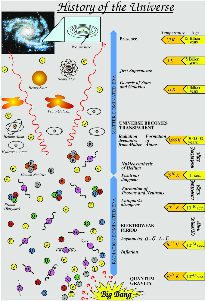
Figure 1.  :

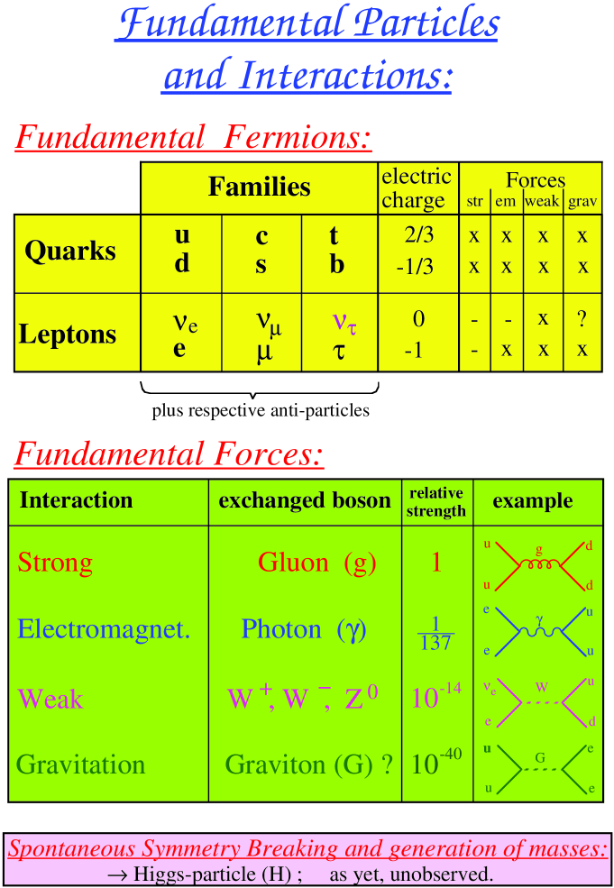
Figure 2.  :

Figure 3.  :

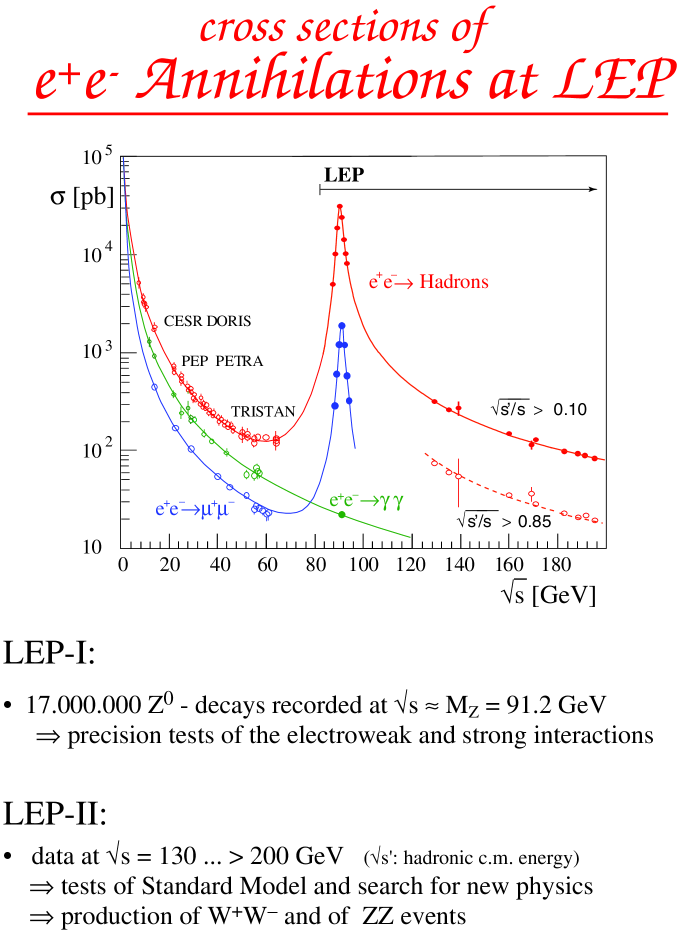
Figure 4.  :

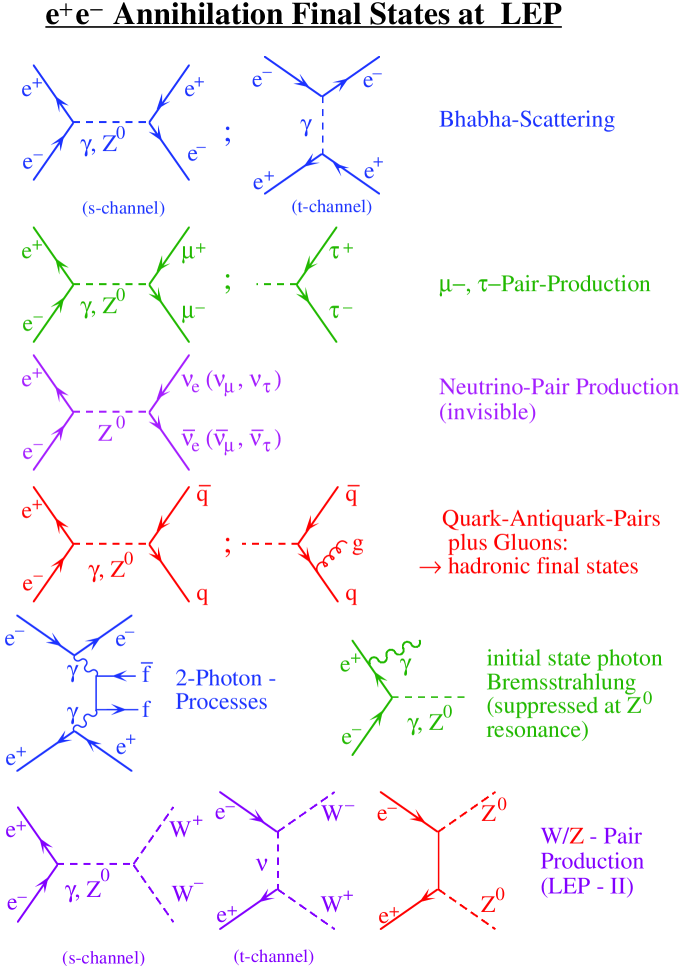
Figure 5.  :

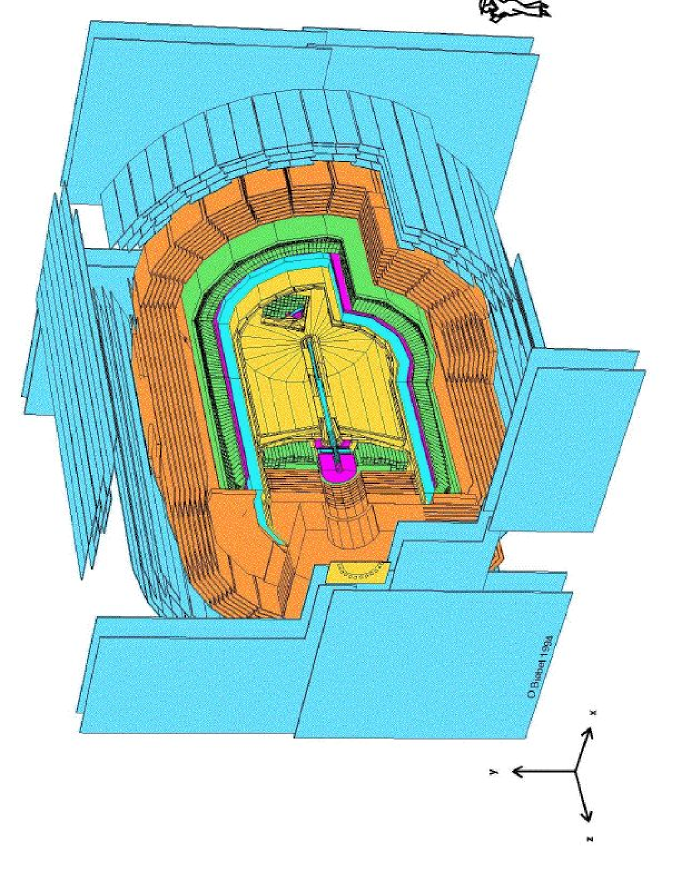
Figure 6.  :

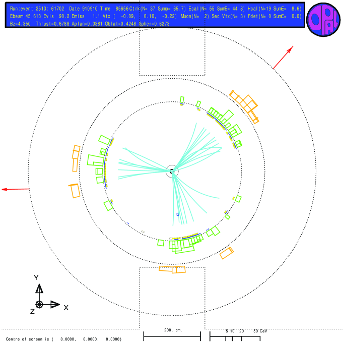
Figure 7.  :

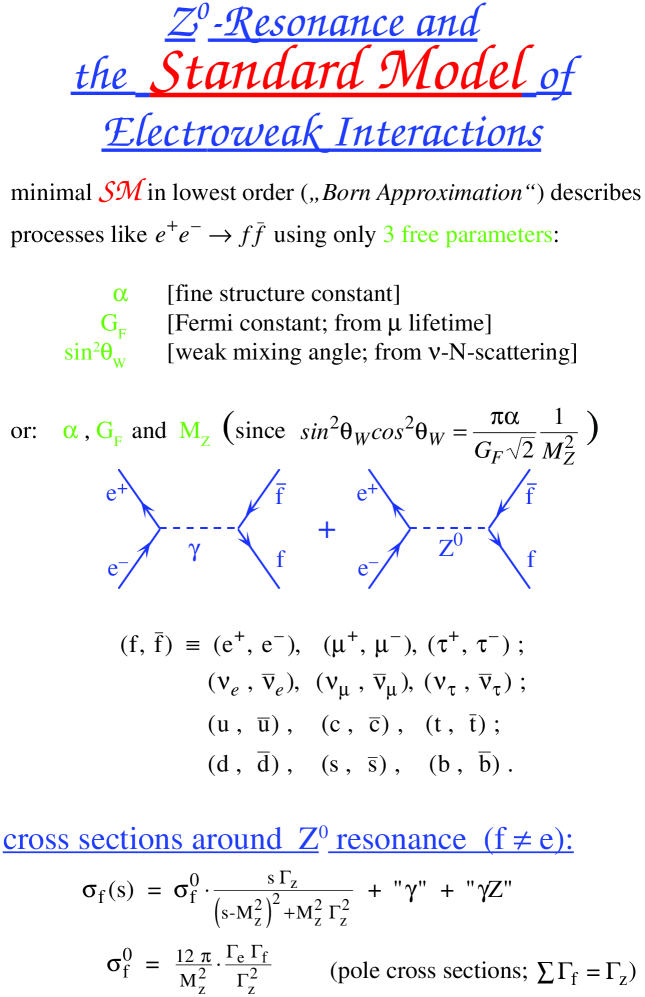
Figure 8.  :

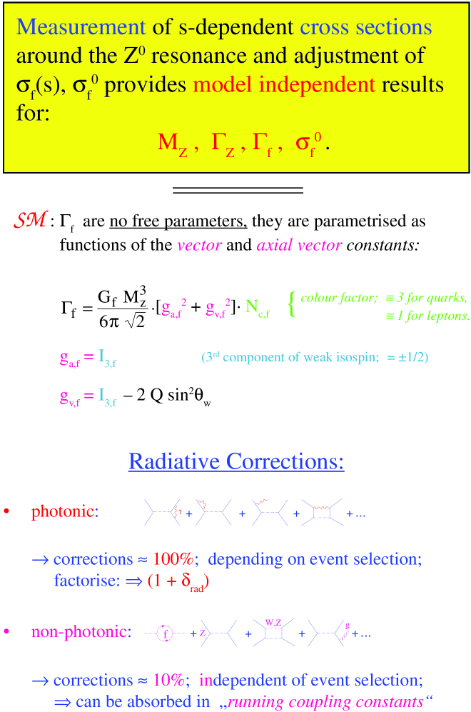
Figure 9.  :

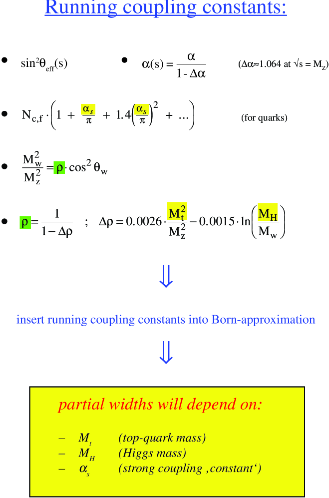
Figure 10.  :

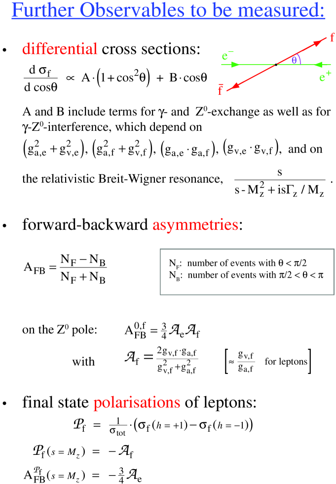
Figure 11.  :

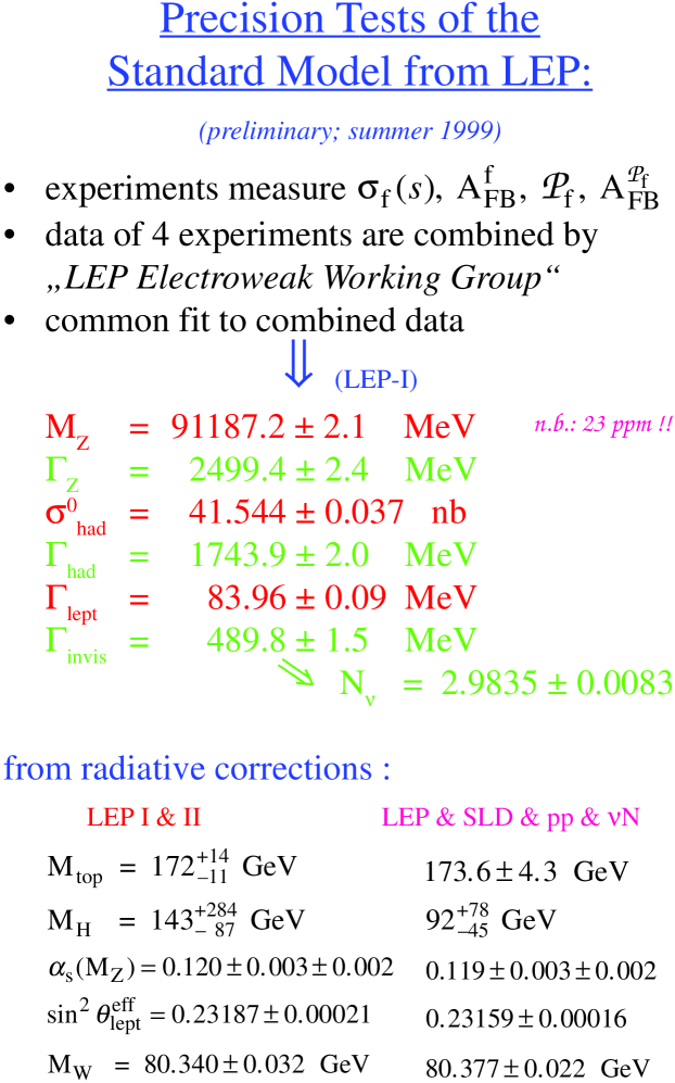
Figure 12.  :

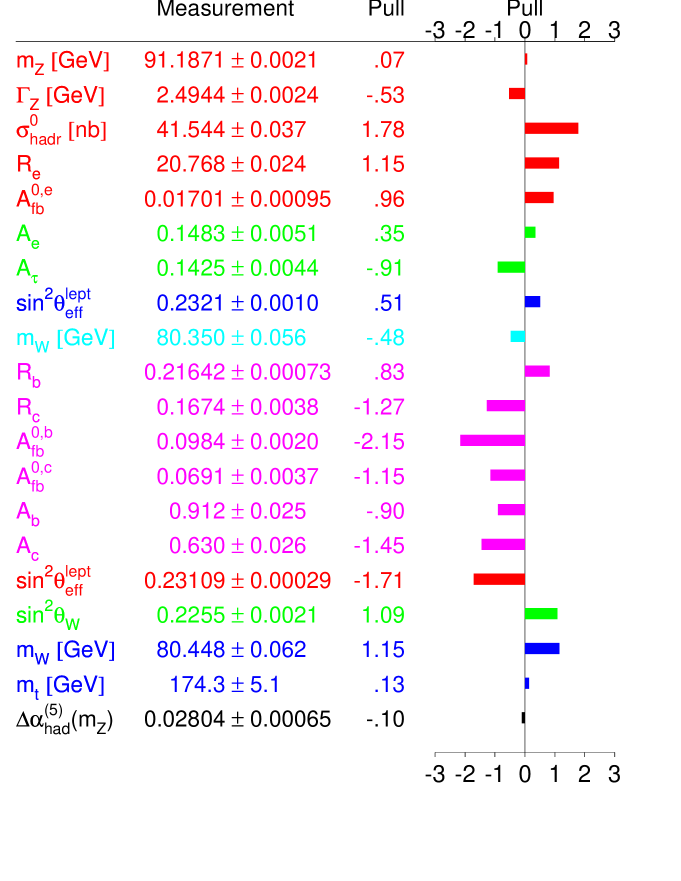
Figure 13.  :

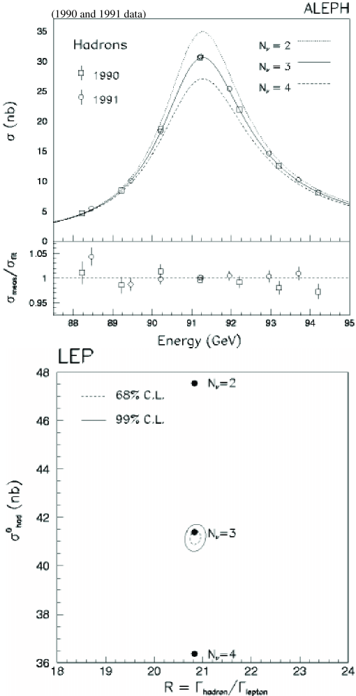
Figure 14.  :

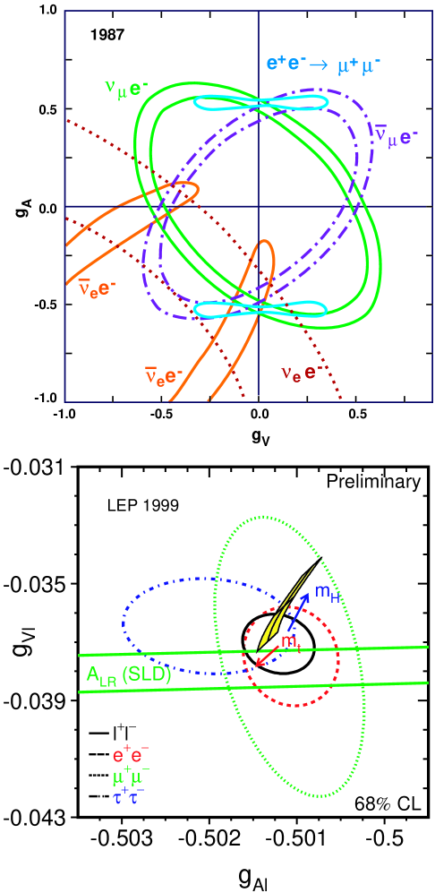
Figure 15.  :

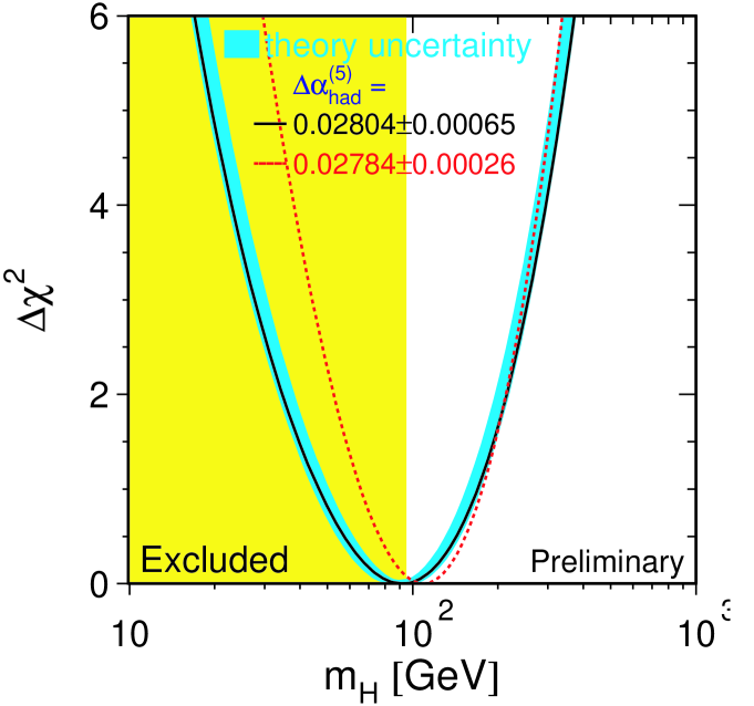
Figure 16.  :

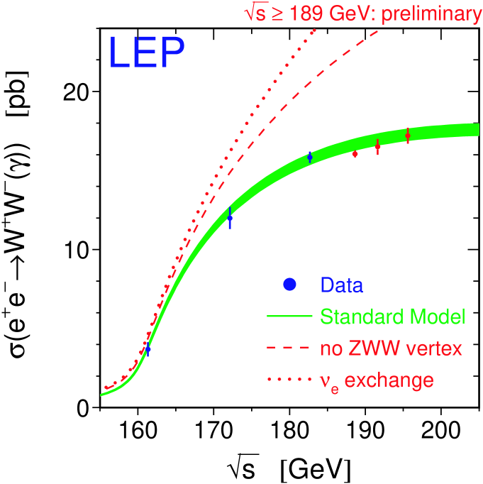
Figure 17.  :

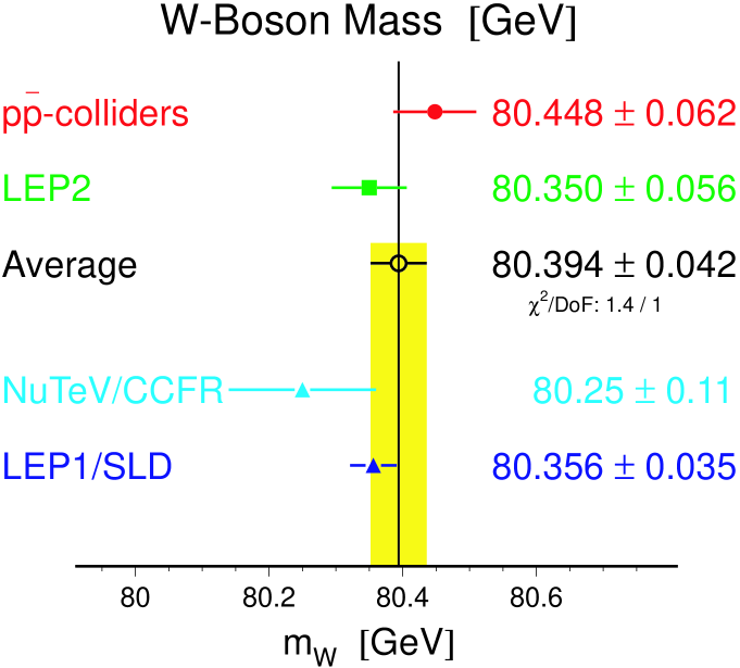
Figure 18.  :

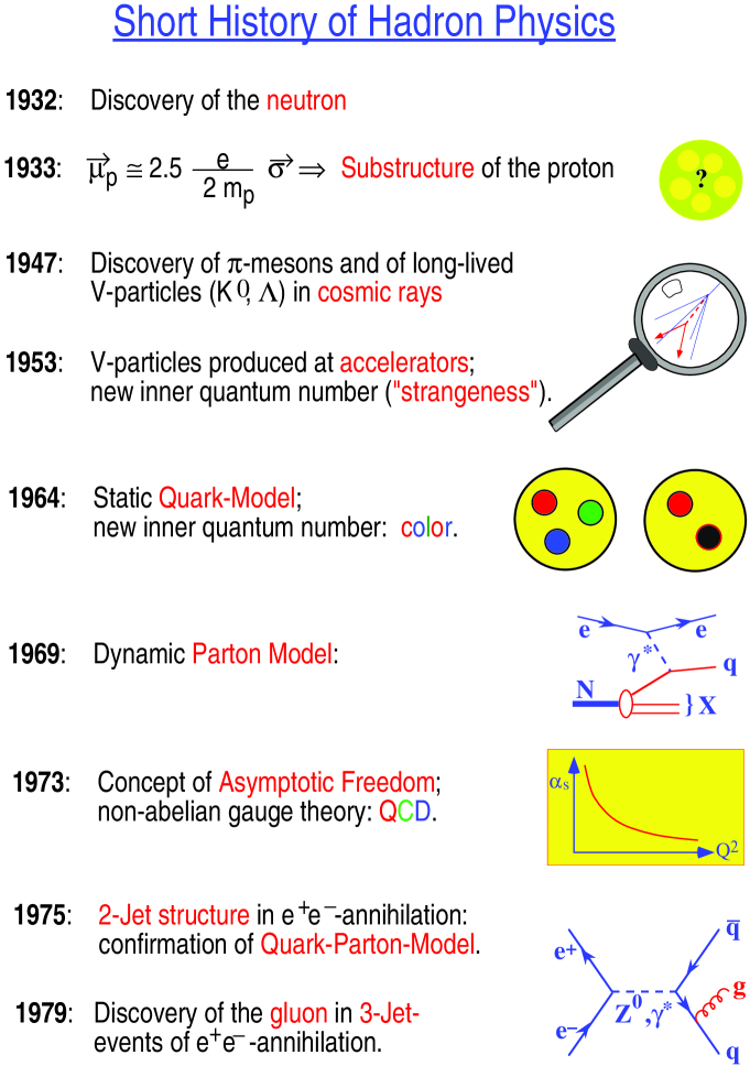
Figure 19.  :

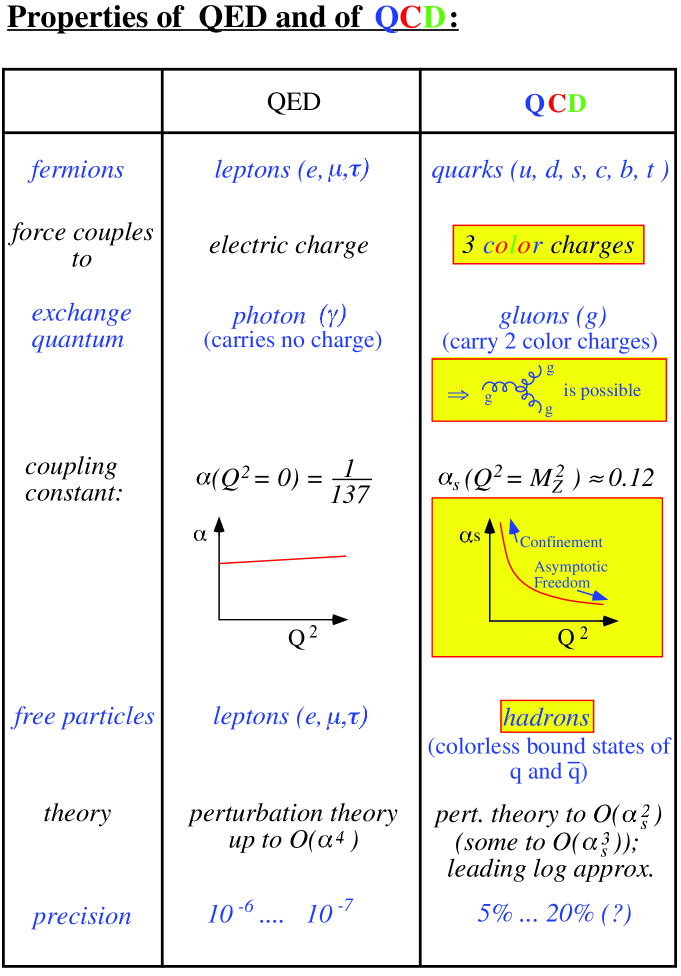
Figure 20.  :

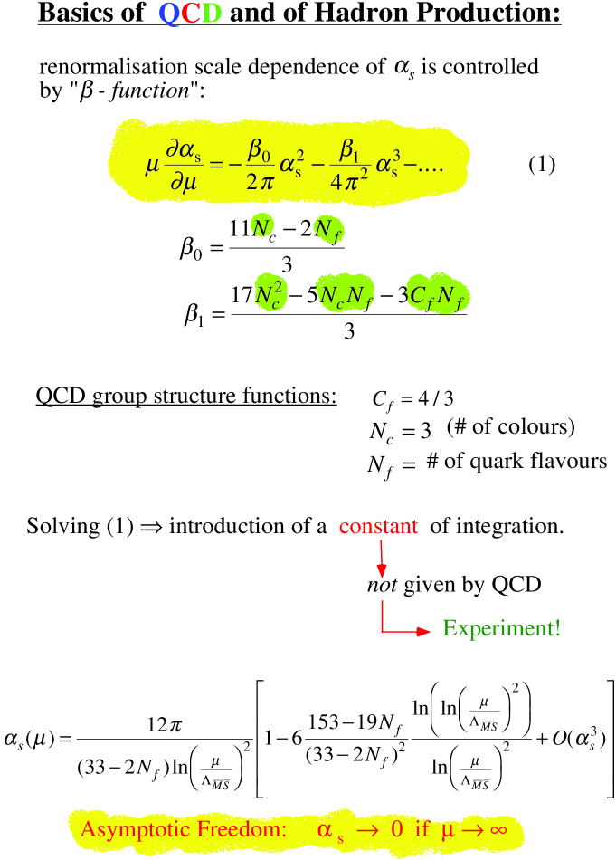
Figure 21.  :

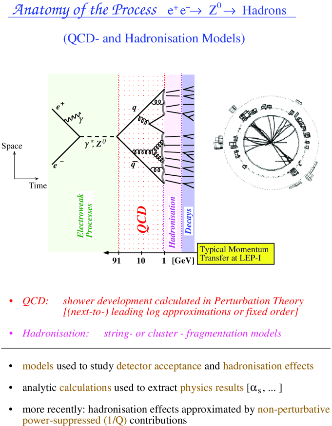
Figure 22.  :

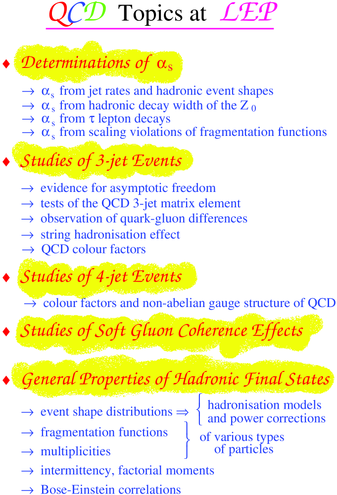
Figure 23.  :

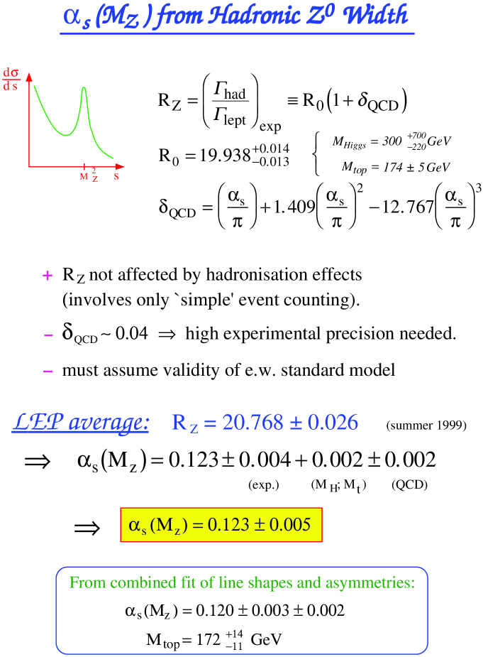
Figure 24.  :

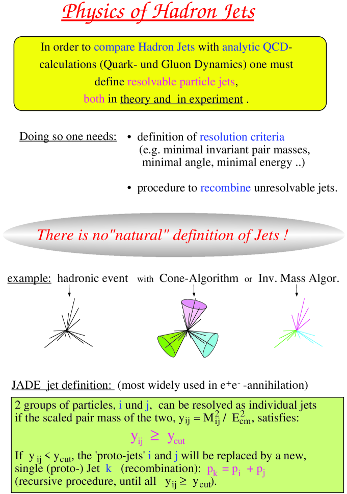
Figure 25.  :

JADE-type Jet Cluster Algorithms

References

-
[1]
see textbooks on Gauge Theories and Particle Physics, as for instance:
E. Leader, E. Predazzi, An Introduction to Gauge Theories and Modern Particle Physics, Vols. 1 and 2, Cambridge University Press, 1996;
C. Quigg, Gauge Theories of the Strong, Weak and Electromagnetic Interactions, Benjamin/Cummings (1983). - [2] S. Myers, E. Picasso, Contemp. Phys. 31 (1990) 387.
- [3] ALEPH Collaboration, D. Buskulic et al., Nucl. Inst. Meth. A360 (1995) 481.
- [4] DELPHI Collaboration, P. Abreu et al., Nucl. Instr. Meth. A378 (1996) 57.
- [5] L3 Collaboration, O. Adriani et al., Phys. Rep. (1993) 236.
- [6] OPAL Collaboration, K. Ahmet et al., Nucl. Inst. Meth. A305 (1991) 275.
- [7] H. Burkhardt, J. Steinberger, Ann. Rev. Nucl. Part. Sci. 41 (1991) 55.
- [8] G. Quast, Prog. Nucl. Part. Phys. 43 (1999) 87.
- [9] J. Mnich, proc. of EPS-HEP’99, Tampere, Finland, July 1999; CERN-EP/99-43.
-
[10]
The LEP Electroweak Working Group, CERN-EP/99-15;
http://www.cern.ch/LEPEWWG/. -
[11]
R. Assmann et al., Eur. Phys. J. C6 (1999) 187;
A. Blondel et al., hep-ex/9901002, subm. to Eur. Phys. J. C. - [12] S. Eidelmann and F. Jegerlehner, Z. Phys. C 67 (1995) 585.
- [13] M. Davier and A. Höcker, Phys. Lett. B419 (1998) 419.
- [14] T. Sjöstrand, hep-ph/9508391.
- [15] G. Marchesini et al., hep-ph/9607393.
- [16] I.G. Knowles and G.D. Lafferty, J. Phys. G23 (1997) 731, hep-ph/9705217.
- [17] R.K. Ellis, W.J. Stirlin and B.R. Webber, QCD and Collider Physics, Cambridge University Pr. (1996).
- [18] S. Bethke, J.E. Pilcher, Ann. Rev. Nucl. Part. Sci. 42 (1992) 251.
- [19] T. Hebbeker, Phys. Rep. 217 (1992) 217.
-
[20]
S. Bethke, Proc. of the Scottish Universities Summer School in
Physics, St. Andrews 1993, in: High Energy Phenomenology, edited by K. Peach and L. Vick, SUSSP Publications and IOP Publishing (1994);
preprint HD-PY 93/7. -
[21]
S.G. Gorishny, A.L. Kataev and S.A. Larin, Phys. Lett. B259 (1991) 144;
L.R. Surguladze, M.A. Samuel, Phys. Rev. Lett. 66 (1991) 560. - [22] T. Hebbeker, M. Martinez, G. Passarino and G. Quast, Phys. Lett. B331 (1994) 165.
-
[23]
JADE Collab., W. Bartel et al., Z. Phys. C33 (1986), 23;
JADE Collab., S. Bethke et al., Phys. Lett. B213 (1988), 235. - [24] Yu.L. Dokshitzer, Contribution to the Workshop on Jets at LEP and HERA, Durham (1990), J.Phys.G17 (1991).
- [25] Z. Kunszt and P. Nason [conv.] in Z Physics at LEP 1 (eds. G. Altarelli, R. Kleiss and C. Verzegnassi), CERN 89-08 (1989).
- [26] S. Bethke, Z. Kunszt, D.E. Soper and W.J. Stirling, Nucl. Phys. B370 (1992) 310.
- [27] Yu.L. Dokshitzer, G.D. Leder, S. Moretti and B.R. Webber, JHEP 9708:001, 1997; hep-ph/9707323.
- [28] S. Bentvelsen and I. Meyer, Eur. Phys. J C4 (1998) 623.
- [29] S. Bethke, Proc. QCD Euroconference 96, Montpellier, France, July (1996), Nucl. Phys. (Proc.Suppl.) 54A (1997) 314; hep-ex/9609014.
- [30] S. Catani, L. Trentadue, G. Turnock and B.R. Webber, Nucl. Phys. B407 (1993) 3.
- [31] L3 Collaboration, M. Acciarri et al., Phys. Lett. B411 (1997) 339.
- [32] P.A. Movilla-Fernandez, O. Biebel and S. Bethke, hep-ex/9906033.
- [33] S. Bethke, Int. Symp. on Radiative Corrections, Barcelona, Sept. 8-12, 1998; hep-ex/9812026.
- [34] K.G. Chetyrkin et al., hep-ph/9706430.
- [35] M. Schmelling, Phys. Scripta 51 (1995) 676.