Abstract

Stars and black holes are sources of gravitational radiation in many phases of their life, and the signals they emit exhibit features that are characteristic of the generating process. Emitted since the beginning of star formation, these signals also contribute to create a stochastic background of gravitational waves. We shall show how the spectral properties of this background can be estimated in terms of the energy spectrum of each single event and of the star formation rate history, which is now deducible from astronomical observations. We shall further discuss the process of scattering of masses by stars and black holes, showing that, unlike black holes, stars emit signals that carry a clear signature of the nature of the source.

1 Introduction

The extraordinary experimental effort done in recent years to design and construct sophisticated and sensitive gravitational antennas, allows to hope that gravitational waves will soon be detected. When this will happen, will we be able to identify the nature of the emitting source, or to decide whether a detected stochastic background was emitted during the early stages of the life of our Universe, or later, by a cosmological population of astrophysical sources? In order to answer these questions, waveforms and energy spectra of the signals emitted in different processess have to be computed and analysed to extract the specific information they provide on the generating process. In this paper we shall discuss some astrophysical phenomena in which this characterization is possible.

Many phases of the life of a star are accompanied by the emission of gravitational waves. For instance, a compact, rotating star emits radiation if it has a time varying quadrupole moment due to a triaxial shape or to a precession of its angular velocity around the simmetry axes. When stellar objects interact, the wave emission can be associated to the orbital motion, or to the excitation of their proper modes of vibration. Further on, intense bursts of radiation can be emitted in catastrophic events such as the gravitational collapse or the coalescence of binary systems. All these processes occurred since the beginning of star formation, and therefore they also contribute to create a stochastic background of gravitational radiation. To evaluate the spectral properties of the contributions of different sources we need a model of the energy spectrum emitted in each single event, as well as the rate of events of the selected type occurred in the recent or far past, i.e. the star formation rate history. As we shall later see, this important piece of information can be deduced from recent astronomical observations.

Among the processes that are associated to the emission of gravitational waves, we shall first consider the final stages of the life of a sufficiently massive star which collapses to form a black hole. In this case numerical simulations show that, unless the collapse is dominated by very strong pressure gradients or by very slow bounces, the newborn black hole wildly oscillates and radiates its residual mechanical energy in gravitational waves, at well defined frequencies and damping times that are associated to its proper modes of vibration: the quasi-normal modes. We will then show how the energy spectrum emitted in each event can be convoluted with the observation-based star formation rate history to compute the spectral energy-density of the resulting background, and we will show that it maintains memory of the quasi-normal mode signature of each collapse. This procedure is applicable to any cosmological population of astrophysical sources for which a model of the emitted energy spectrum is available.

Another interesting astrophysical process that is associated to a well characterized signal is the scattering of a mass by the gravitational field of a massive body, either a compact star or a black hole. We shall describe how the energy spectra and waveforms can be computed in the framework of a perturbative approach, and show that the gravitational signals carry a specific information on the nature of the emitting source.

2 The gravitational collapse to a black hole

In 1939, Oppenheimer & Snyder [1] studied the collapse of a spherical cloud of a pressureless gas of particles (dust), and showed that once the collapsing cloud reaches the horizon, it cuts the communications with the external world and forms a black hole. In that case, due to the assumed spherical symmetry, no gravitational radiation emerged. However, gravitational waves are emitted if the collapsing configuration deviates from sphericity, and this is the basic idea of a perturbative approach introduced by C.T. Cunningham, R.H. Price and V. Moncrief [2, 4] and subsequently applied by E. Seidel and T. Moore [5, 6] (for a recent review see [7]). The perturbative approach consists in the following. Due to a sudden change in some equilibrium variable, a sperically symmetric compact star with an assigned equation of state collapses. Typically, the pressure is changed so that the star is no longer in equilibrium. The collapsing configuration is obtained by numerically integrating the Einstein equations coupled to the equations of hydrodynamics, and this exact solution - ‘exact’ in the sense that it is a solution of the fully non-linear equations - is used as a background about which linear perturbations are considered. The perturbed equations, derived in the framework of a gauge invariant formalism [2, 4], are then numerically integrated to compute the energy spectrum and the waveforms.

Alternatively, the gravitational collapse can be studied by directly integrating the fully non-linear equations of gravity, and at present there is only one fully relativistic numerical simulation of collapse to a black hole. In 1985 R. Stark and T. Piran [8] numerically integrated the equations describing the collapse of a rigidly rotating, axisymmetric polytropic star. Although this simulation is based on some simplifying assumptions, it can be considered as a good model to extract information on the collapse of a massive star to a black hole; indeed, it has be shown that the spectrum of the emitted gravitational energy exhibits some distinctive features that are, to some extent, independent of the initial conditions and of the equation of state of the collapsing star, and that depend only on the black hole mass and on its angular momentum.

The dynamics of the collapse proceeds as follows. If the total angular momentum  $a=\frac{J}{\frac{GM^{2}}{c}}$  is greater than a critical value  $a_{crit}$  the rotational energy dominates, the star bounces and no collapse occurs. Conversely, if  $a<a_{crit}$  a black hole forms.

Figure 1: The  $h_{+}$  component of the gravitational radiation (a) and the average energy flux per unit frequency (b) emitted during the axisymmetric collapse of a rotating, polytropic star to a black hole, are plotted for assigned value of the angular momentum [8]. These data refer to a collapse ignited by a pressure reduction to a fraction  $f_{p}=0.01$ of the equilibrium central pressure.

In figure 1a we plot the waveform, i.e. the  $h_{+}$-component of the metric tensor of the gravitational wave emerging at infinity, evaluated in the TT-gauge. The  $h_{\times}$-component is much smaller and does not significantly contribute to the emitted radiation. The function  $f(\nu)$  plotted in figure 1b is an average energy flux computed as follows

$$f(\nu)=\frac{1}{4\pi r^{2}}\int_{0}^{2\pi}d\phi\int_{0}^{\pi}\left(\frac{dE_{GW}}{d\nu d\Omega}\right)\sin\theta d\theta.$$ (1)

The amplitude of  $f(\nu)$  scales as the fourth power on the angular parameter  $a,$  and it is proportional to the square of the mass of the collapsing core; the efficiency of the process is $\Delta E_{GW}/M_{core}c^{2}\leq 7\times 10^{-4}$.

Figure 1b shows that if the angular momentum increases more energy is emitted in the low frequency region. This is due to the fact that for high values of  $a$  the star becomes flattened into the equatorial plane, and bounces vertically before collapsing. However, the more distinctive feature of these energy spectra is the peak which occurs at a frequency that depends on the angular parameter; for instance  $\nu_{max}\simeq 8.7$  for  $a=0.79,$  and  $\nu_{max}\simeq 9.0~{}kHz$  for  $a=0.94.$  Moreover, the ringing tails exhibited by the waveforms plotted in figure 1a are damped sinusoids at these frequencies. In order to understand what is the physical phenomenon which associated to the emission of these peaks, we need to define the quasi-normal modes of black holes, that emerge from the theory of black hole perturbations [9].

2.1 The perturbations of a rotating black hole

It is known that the radial evolution of the perturbations of a rotating black hole is described by a single master equation for a radial wavefunction  $R_{lm}(r,\omega)$:

$$\Delta\frac{\partial^{2}R_{lm}}{\partial r^{2}}+2(s+1)(r-M)\frac{\partial R_{lm}}{\partial r}+V(r,\omega)R_{lm}=0,$$ (2)

where

$$V(r,\omega) = \frac{1}{\Delta}\Biggl{\{}(r^{2}+a^{2})^{2}\omega^{2}-4aMrm\omega+a^{2}m^{2}+2is\Bigl{[}am(r-M)\Biggr{.}\Bigr{.}$$

$$- \Biggl{.}\Bigl{.}M\omega(r^{2}-a^{2})\Bigr{]}\Biggr{\}}+\Biggl{[}2is\omega r-a^{2}\omega^{2}-A_{lm}\Biggr{]}$$

$$\Delta = r^{2}-2Mr+a^{2},$$

$s$  is the spin-weight parameter,  $s=0,\pm 1,\pm 2$  respectively for scalar, electromagnetic and gravitational perturbations, and the sign indicates whether the ingoing or outgoing radiative part of the field are considered.  $A_{lm}$  is a separation constant. This wave equation was derived by S. Teukolsky in 1972 [10, 11]. The quasi-normal modes of a black hole are defined to be complex frequency solutions of the wave equation 2, that behave as a pure outgoing wave at infinity, where radiation has to emerge, and as a pure ingoing wave at the horizon, since nothing can escape from a black hole horizon. The eigenfrequency of a mode is complex because the emitted radiation damps the oscillations, and the real part is the pulsation frequency, whereas the imaginary part is the inverse of the damping time. Numerical integrations of the wave equations have shown that these frequencies are characteristic of many processes involving dynamical perturbations of black holes, and that an initial perturbation decays, during its very last stages, as a superposition of these pure modes. In table 1 we tabulate the characteristic frequency of the lowest quasi-normal mode of a rotating black hole, for  $\ell=2$  and  $m=0,$  computed by Leaver [12]. The corresponding values in physical units can be evaluated by using the following formulae

$$\nu_{0}=\frac{c(M\omega_{0})}{2\pi n\cdot M_{\odot}}=\frac{32.26}{n}(M\omega_{0})kHz,$$ (4)

$$\tau=\frac{nM_{\odot}}{(M\omega_{i})c}=\frac{n\cdot 0.4937\cdot 10^{-5}}{(M\omega_{i})}~{}s.$$

where  $M_{\odot}=1.48\cdot 10^{5}cm$  and we have assumed that the black hole mass is  $M=nM_{\odot}.$

Table 1: The characteristic frequency of the first quasi-normal mode of a rotating black hole is tabulated, for  $\ell=2$  and  $m=0,$  for different values of the angular parameter  $a.$

$a$	${M\omega_{0}+iM\omega_{i}}$
0.0	0.3737+i0.0890
0.2	0.3751+i0.0887
0.4	0.3797+i0.0878
0.6	0.3881+i0.0860
0.8	0.4019+i0.0822
0.9	0.4120+i0.0785
0.98	0.4223+i0.0735
0.9998	0.4251+i0.0718

Thus we easily find that for  $\ell=2$

$$a=0.79\qquad\nu_{0}=8.6~{}~{}kHz,\qquad\quad a=0.94\qquad\nu_{0}=9.0~{}~{}kHz.$$

If we now go back to the energy spectra plotted figure 1b, we see that they peak at a frequency which is very close to  $\nu_{0},$  i.e. to the frequency of the lowest  $m=0$  quasi-normal mode of the rotating black hole which forms as a result of the collapse. It should be mentioned that the excitation of the quasi-normal modes also emerges in simulations of the collapse to a black hole done in the framework of perturbative approaches. Thus, the quasi-normal mode peak is a specific signature of the emitted energy spectrum, since it indicates that the newborn black hole oscillates in these modes, releasing its mechanical energy in the form of gravitational waves.

We may ask to what extent is this signature a general feature of the signals emitted during the collapse of a sufficiently massive star to a black hole. A study done by E.Seidel using the perturbative approach [13], has shown that if the collapse is dominated by extremely high pressures or by slow bounces, the infalling material can be considerably slowed down and the formed black hole may be left with very little residual energy to radiate away in gravitational waves. In this case the quasi-normal modes peak may not be as pronounced as in figure 1b. However, these are quite extreme situations, and it is reasonable to presume that the gravitational collapse will leave behind a newborn black hole with some residual mechanical energy, which will be radiated in gravitational waves at the frequencies of the black hole quasi-normal modes. The efficiency of the gravitational emission evaluated by Stark and Piran has to be taken as an indication: it may be smaller, if strong pressures and slow bounces dominate the collapse, but it may also be higher, if the collapse is non-axysimmetric.

3 From a single event to a stochastic background

The gravitational signals emitted by newly formed black holes throughout the Universe superimpose to form a stochastic background. In order to evaluate the spectral properties of this background and verify whether it keeps memory of the generating process, besides the energy spectrum emitted in each single event, we need to know the rate of events as a function of the cosmological redshift. This information can be deduced from the observative data collected by the Hubble Space Telscope, Keck and other large telescopes [14]-[15], which, together with the completion of several large redshift surveys [16]-[17] have enabled to derive coherent models for the star formation rate evolution up to redshifts of $\sim 4-5$.
In figure 2 we plot a recently proposed fit of the data obtained at different redshifts, representing the star formation rate density  ${\dot{\rho}_{\star}(z)},$  which is the mass of gas which forms stars per unit time and comoving volume element [18], [15]. The observative data-points use the rest-frame UV-optical luminosity as an indicator of the star formation activity in distant galaxies, and it is known that even a relatively small amount of dust can absorbe the UV light and reradiate it in the far-IR. This causes an attenuation of the observed UV-luminosity (dust extinction) and leads to an underestimate of the real star formation activity. To account for this problem, the data shown in fig. 2 have been corrected according to the Calzetti dust extinction law (see [19], [15]).

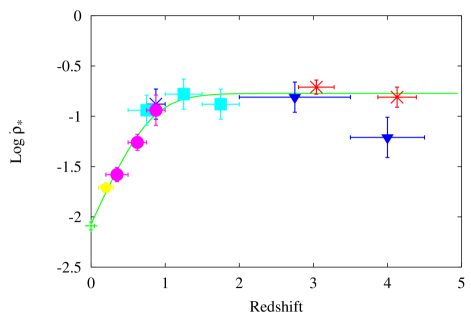
Figure 2: The star formation rate density in units of $M_{\odot}\mbox{yr}^{-1}\mbox{Mpc}^{-3}$ is plotted as a function of redshift for a cosmological background model with $\Omega_{M}=1$, $\Omega_{\Lambda}=0$, $H_{0}=50\,\mbox{km}\mbox{s}^{-1}\mbox{Mpc}^{-1}$ and a Salpeter initial mass function.

The amount of dust correction to be applied at intermediate-to-high redshift $z\!\stackrel{{\scriptstyle\scriptscriptstyle>}}{{\scriptscriptstyle\sim}}\!1-2$, is still relatively uncertain. However, since the energy emitted by a single source decreases as the square of the inverse of the luminosity distance, the gravitational wave backgrounds generated by astrophysical sources are almost insensitive to the high redshift behaviour of the star formation rate. Using the function  ${\dot{\rho}_{\star}(z)}$  plotted in fig. 2, the rate of core-collapse supernovae can be computed as follows [20]

$$R(z)=\int_{0}^{z}dz^{\prime}\,\frac{\dot{\rho}_{\star}(z^{\prime})}{1+z^{\prime}}\,\frac{dV}{dz}\,\int_{\Delta M}\!\!dM^{\prime}\,\Phi(M^{\prime}).$$ (5)

The the factor $(1+z)^{-1}$ takes into account the dilution due to cosmic expansion and $\Phi(M)$ is the initial mass function chosen to be of Salpeter type, $\Phi(M)\propto M^{-(1+x)}$ with $x=1.7$.
The mass range,  $\Delta M,$  depends on the nature of the considered source. Numerical studies on stellar evolution have shown that single stars with mass exceeding $~{}\!8M_{\odot}$ evolve through all phases of nuclear burning, ending their life as core collapse supernovae (this class includes Type II and Types Ibc supernovae). While there seems to be a general agreement that progenitors with masses in the range $8M_{\odot}\!\stackrel{{\scriptstyle\scriptscriptstyle<}}{{\scriptscriptstyle\sim}}\!M\!\stackrel{{\scriptstyle\scriptscriptstyle<}}{{\scriptscriptstyle\sim}}\!20M_{\odot}$ leave neutron star remnants, the value of the minimum progenitor mass which leads to a black hole is still uncertain, mainly because of the unknown amount of fall back of material during the supernova explosion [21], [22]. In the following we shall assume that the lower threshold for black hole formation is  $M\!\stackrel{{\scriptstyle\scriptscriptstyle>}}{{\scriptscriptstyle\sim}}\!25~{}M_{\odot}$.

The rate of events (5) depends also on the cosmological background through the comoving volume element

$$dV=4\pi\left(\frac{c}{H_{0}}\right)\,r^{2}\,\frac{1}{\sqrt{(1+z)^{2}\,(1+\Omega_{M}\,z)-z\,(2+z)\,\Omega_{\Lambda}}}\,dz,$$ (6)

where  $r$  is the comoving distance

$$r=\frac{c}{H_{0}\sqrt{\Omega_{\kappa}}}\cdot S\Bigl{(}\sqrt{\Omega_{\kappa}}\,\int_{0}^{z}[(1+z^{\prime})^{2}\,(1+\Omega_{M}\,z^{\prime})-\\ z^{\prime}\,(2+z^{\prime})\,\Omega_{\Lambda}]^{-1/2}\,dz^{\prime}\Bigr{)},$$

and the function  $S$  is given by [23]

$$\Omega_{M}+\Omega_{\Lambda}>1 \quad S(x)=\sin(x) \quad\Omega_{\kappa}=1-\Omega_{M}+\Omega_{\Lambda}$$ (7)

$$\Omega_{M}+\Omega_{\Lambda}<1 \quad S(x)=\sinh(x) \quad\Omega_{\kappa}=\Omega_{M}+\Omega_{\Lambda}-1,$$

$$\Omega_{M}+\Omega_{\Lambda}=1 \quad S(x)=x \quad\Omega_{\kappa}=1.$$

If we consider the following cosmological backgrounds

$$A) \Omega_{M}=1 \Omega_{\Lambda}=0\qquad h=0.5$$ (8)

$$B) \Omega_{M}=0.3 \Omega_{\Lambda}=0.7\qquad h=0.6$$

$$C) \Omega_{M}=0.4 \Omega_{\Lambda}=0\qquad h=0.6$$

the total rate of core-collapse supernovae leading to a black hole or to a neutron star ranges, respectively, between

$$R_{BH}~{}\sim 3.3-4.7~{}events/s,\qquad R_{NS}~{}\sim~{}13.6-19.3~{}events/s.$$ (9)

The main difference between the three cosmologies is introduced by the geometrical effect of the comoving volume, and it is significant at $z\!\stackrel{{\scriptstyle\scriptscriptstyle>}}{{\scriptscriptstyle\sim}}\!1-2$. This implies that the gravitational backgrounds, which are mainly contributed by sources at $z\!\stackrel{{\scriptstyle\scriptscriptstyle<}}{{\scriptscriptstyle\sim}}\!1-2$, are almost insensitive to the cosmological parameters.
It is now possible to compute the spectral energy density of the gravitational wave background produced by an assigned population of sources

$$\frac{dE\left(\nu\right)}{dtdSd\nu}=\int^{0}_{\infty}\int_{\Delta M}~{}\Biggl{[}f(\nu)\cdot dR(z,M)\Biggr{]},$$ (10)

where  $dR(z,M)$  is the differential rate, and  $f(\nu)$  is the average energy flux per unit frequency, chosen as a model for the class of sources under consideration, emitted by a source located at a luminosity distance  $d_{L}(z)=(1+z)~{}r,$

$$f(\nu)=\frac{1}{4\pi d_{L}(z)^{2}}\int_{0}^{2\pi}d\phi\int_{0}^{\pi}\left(\frac{dE_{GW}}{d\nu d\Omega}\right)\sin\theta d\theta.$$ (11)

For instance, for core collapses to a black hole we shall use as a model of  $f(\nu)$  the energy spectrum (1) shown in figure 1b, rescaled with the luminosity distance and suitably redshifted.

From eq. (10) we can further derive the closure energy density of gravitational waves per logarithmic unit frequency,

$$\Omega_{GW}=\frac{1}{\rho_{c}}\cdot\frac{d\rho_{GW}}{d\log\nu}=\frac{\nu}{c^{3}\rho_{c}}\cdot\frac{dE_{GW}}{dtdSd\nu}$$ (12)

where  $\rho_{c}=\frac{3H_{0}^{2}}{8\pi G}\sim 1.9\times 10^{-29}~{}h^{2}~{}g~{}cm^{-3},$  and the spectral strain amplitude

$$\sqrt{S_{h}(\nu)}=\Biggl{[}\Bigl{(}\frac{2G}{\pi c^{3}\nu^{2}}\Bigr{)}\cdot\frac{dE_{GW}}{dtdSd\nu}\Biggr{]}^{1/2}=\Biggl{[}\Bigl{(}\frac{3~{}H_{0}^{2}}{4\pi^{2}\nu^{3}}\Bigr{)}\cdot\Omega_{GW}\Biggr{]}^{1/2},$$ (13)

which is the quantity to be compared with the detectors sensitivity. The spectral properties of the background produced by a cosmological populations of core-collapse supernovae leaving behind a black hole, computed by this procedure, are shown in figure 3. We plot the closure energy density and the strain amplitude for three selected values of the angular parameter of the formed black holes, assumed to rotate all at the same speed since we do not know the distribution of black holes angular momenta.

Figure 3: The closure energy density  $\Omega_{GW}$  (left) and the spectral strain amplitude  $S_{h}^{1/2}$  (right) generated by a cosmological population of core collapse supernovae leaving behind a black hole, is plotted as a function of the observational frequency, for three values of the angular parameter $a$ and for a flat cosmology with vanishing cosmological constant.

The strain amplitude exhibits a sharp peak at a frequency which ranges within $\sim~{}[230-340]~{}Hz,$  depending on the chosen value of the angular momentum, and with a maximum amplitude  $\sqrt{S_{h~{}max}}\sim[1-8]~{}\times 10^{-28}~{}Hz^{-1/2}.$  This peak is reminiscent of the excitation of the quasi-normal modes of the formed balck holes, showing that the spectral properties of this background keeps memory of the generating process.

It should be mentioned that since according to eq. (9) the event rate is of the order of  $3-5~{}events/s,$  and since a signal emitted in a collapse to a black hole has a very short durations (cfr. eq. 4), typically of the order of a few milliseconds, the background generated by newborn black holes has a shot noise character.

The procedure to determine the characteristics of a stochastic background described in this section can be applied to any population of astrophysical sources for which a model for the energy spectrum is available. For example, in ref. [24] we have applied this method to study the background produced by a cosmological population of young, rapidly rotating neutron stars that, due to the r-modes instability, are expected to radiate a large fraction of their rotational energy in gravitational waves. A gravitational background can be detected by cross-correlating the output of two gravitational antennas for a sufficiently long time interval (typically one year), and in refs. [20] and [24] we have computed how interferometric and resonant detectors operating in coincidence might respond to our predicted astrophysical backgrounds. We find that whereas the sensitivity of the first generation of interferometric antennas like VIRGO and LIGO will be too low to detect these signals, the planned sensitivity of the advanced version of these experiments would allow the detection, provided two interferometers with similar characteristics are located nearby.

4 Gravitational waves from stars: a perturbative approach

A number of numerical simulations of the gravitational collapse to a neutron star have shown that, unlike the case of collapses to a black hole, the gravitational signals computed for these processes strongly depend on the initial conditions, on the equation of state of the collapsing star, and on the details of the collapse [25]-[27]; for this reason, a model of the energy spectrum emitted in a collapse to a neutron star is still not available. The situation changes if we consider processes occurring after a neutron star has formed, and we shall now show how some interesting information can be derived by using a perturbative approach.

The theory of stellar perturbations was formulated in the framework of General Relativity by Thorne and his collaborators since 1967 [28]-[33], and it was successfully applied to determine the frequencies of the quasi-normal modes of oscillation for a wide range of stellar models [34, 35]. Much recently, the theory has been reformulated in close analogy to the theory of black hole perturbations [36]-[43], and new phenomena have emerged, which do not have a newtonian counterpart. A detailed discussion of the many interesting aspects of this theory is beyond the scope of this paper, where we want to focus essentially on the characteristics of the gravitational signals emitted in astrophysical processes. Thus, we shall rather consider an application of the theory to a specific process, and show that the emitted signals exhibit a clear signature of the nature of the source. In particular, we shall consider a mass  $m_{0}$  which, interacting with the gravitational field of a star of mass  $M$  deviates from its original trajectory moving toward the star, reaches a periastron (the turning point) and then moves away in an open orbit. Under the assumption that  $m_{0}<<M,$  the problem can be solved by using a perturbative approach. The matching of the solutions of the perturbed equations inside and outside the star constitutes the most delicate technical point [44]. Indeed, while the interior solution is found by integrating the equations for the perturbed metric tensor coupled with the equations of hydrodynamics, the exterior solution cannot be found by using the same tensorial approach because the source term of the equations for the scattered mass diverges at the turning point. However this difficulty can be overcome by introducing a suitable wavefunction, related to the Weyl scalar  $\Psi_{4},$  which carries information on the radiative part of the field. In ref. [45] the equations describing the perturbations of a star induced by a scattered mass, have been integrated for a star with a polytropic equation of state  $p=K\rho^{n},$  with  $K=100~{}km,$    $n=2,$  and central density  $\rho_{c}=3\cdot 10^{15}~{}g/cm^{3}.$  The radius and mass of the star are, respectively,  $R=8.86~{}km,$  and  $M=1.266~{}M_{\odot},$  with a ratio  $R/M=4.7$

Figure 4: The  $\ell=m=2$ - component of the energy spectrum of the gravitational radiation emitted when a mass  $m_{0}$  is scattered by a polytropic star of mass  $M,$ is plotted versus the normalized frequency  $\omega M$  . The orbital parameters  $L$  and  $E$  are chosen in such a way that the turning point is at  $r_{t}=9.2~{}M$  (a) and  $r_{t}=5~{}M$  (b)

The energy spectrum emitted in gravitational waves has been computed for the following sets of orbital paramenters

• a)    $L=5$  and  $E=1.007,$  which correspond to a turning point located at  $r_{t}=9.2~{}M$

• b)    $L=5$  and  $E=1.097,$  so that the mass can get closer to the star and  $r_{t}=5.0~{}M,$

and it is plotted in figure 4 versus the normalized frequency  $\omega~{}M.$ $L=L_{z}/M$  is the angular momentum of the scattered mass  $m_{0},$  normalized to $M$, and  $E$  is its energy per unit mass.

Figure 4 shows that the energy spectra exhibit well defined peaks located at some particular frequencies, and in order to understand the physical processes that underlie this structure we need to mention what are the characteristic frequencies at which a star can oscillate and possibly emit gravitational waves.

In newtonian theory, the classification of the modes of oscillations of a star is based on the behaviour of the perturbed fluid. The hydrodynamical equations show that when a star is perturbed each element of fluid moves under the competing action of two restoring forces, one due to the eulerian change in the density $\delta\rho$, the other due to a change in pressure $\delta p$. The modes are classified accordingly: g modes, if the prevailing driving force is due to $\delta\rho$, p modes, if it is due to $\delta p$. The two classes of modes occupy well defined regions of the spectrum, and they are separated by the fundamental mode, the f mode, characterized by having an eigenfunction that has no nodes inside the star. In General Relativity stellar oscillations are damped by the emission of gravitational waves, and in addition to the fluid modes there exist modes of the radiative field. Indeed, it can be shown that fluid motion is either negligible or totally absent at the corresponding frequencies. They are named w modes, characterized by high frequencies and short damping times [46], and s modes, that are slowly damped, do not excite any motion in the fluid and are characteristics of ultracompact stars ($R/M\!\stackrel{{\scriptstyle\scriptscriptstyle<}}{{\scriptscriptstyle\sim}}\!2.6$) [39].

Thus, stars are characterized by a very rich set of possible modes of vibration, and it is interesting to ask whether these modes can be excited in real astrophysical processes, and how much energy they carry. For example, for the model of star considered in figure 4 the frequency of the fundamental mode is  $\omega~{}M=0.120,$  the first p -modes is  $\omega~{}M=0.266$  and the first w-mode is  $\omega~{}M=0.53.$  The energy spectra of figure 4 exhibit a pronounced peak at the frequency of the f mode, and more peaks appear, corresponding to the excitation of the first p -modes, if the scattered mass is allowed to get closer.

It is interesting to compare this behaviour with that of a black hole perturbed by a small mass in a similar scattering process (see [47] for an extensive review). It turns out that the black hole is rather insensitive to these processes: the energy is emitted essentially by the scattered mass as a synchrotron radiation, and most of it is radiated when the mass transits through the turning point. Indeed, the energy spectrum is peaked at a frequency which is related to the angular velocity of the mass at the turning point as follows

$$\omega_{r_{t}}=\ell\Bigl{(}\frac{d\varphi}{dt}\Bigr{)}_{r=r_{t}}.$$ (14)

In our case a) ($r_{t}=9.2M$), the frequency corresponding to the angular velocity of the mass at the periastron for  $\ell=2$  is  $\omega_{r_{t}}M=0.092.$  The spectrum shown in figure 4a has a peak at that frequency, showing that part of the energy is still emitted by the mass as a synchrotron radiation, but the the very sharp peak which occurs at the frequency of the fundamental mode is dominant. A similar situation arises when the mass gets closer to the star (case b, $r_{t}=5M$, $\omega_{r_{t}}M=0.221$), but again the emission is strongly dominated by the excitation of the modes of the star. Thus, we can conclude that, unlike black holes, whose quasi-normal modes are not excited in scattering processes, a mass moving around a star in an open orbit can excite the fluid modes of the star, to an extent that depends on how close is the encounter. The w-modes do not appear to be significantly excited in these processes, and since the contribution of the fundamental mode appears to be the dominant one, the emitted gravitational signal is a pure note corresponding to that frequency.

5 Concluding Remarks

The study of the gravitational radiation emitted by astrophysical sources is an open field to explore, and it requires the cooperative effort of scientists working in different fields. Complex phenomena like the gravitational collapse of a massive body or the coalescence of binary systems are paradigmatic: powerful computers and specific expertise in numerical techniques to deal with the strong field regimes typical of these processes are needed, as well as experience in the physics of phenomena occurring at supernuclear densities and a deep mathematical knowledge of the equations of gravity. In addition, since to detect a signal it is important to know not only the waveform and the energy it carries, but also the rate of occurrence, the knowledge of the sources distribution and evolution throughout the Universe, either theoretical or based on observations, is also crucial.

Although most of the interesting phenomena that are associated to the emission of gravitational radiation are highly non linear, much can be learnt by the use of approximation schemes. For instance the perturbative approach proves extremely useful in providing a physical understanding of many processes; it helps to interpret and confirm the results of fully non linear simulations, and to identify physical mechanisms operating in different regimes. An example of this synergy of the approaches is given in section 2, where the peaks of the energy spectrum emitted in a collapse to a black hole, computed by a fully relativistic numerical simulation, have been interpreted in terms of the excitation of the quasi normal modes predicted by the theory of black hole perturbations.

Furthermore, we have shown how theory and observations can be matched together to evaluate the spectral properties of the background of gravitational waves produced by these sources: the energy spectrum of each single event derived by numerical simulations has been convoluted with the star formation rate history deduced from astronomical observations.

The work presented in this paper can be extended in several directions. We plan to apply the procedure developed to evaluate the background of gravitational waves to other cosmological populations of astrophysical sources, like binary systems formed by neutron stars, black holes and white dwarfs [48]. Furthermore, we shall compute energy and waveforms of the signals emitted by stars perturbed by masses orbiting in closed orbits, and investigate the relation between the amplitude of the emitted wave and the equation of state prevailing in the star interior, for different star models ranging from sun-like stars to white dwarfs and neutron stars. Finally, we plan to investigate the role that the excitation of the quasi-normal modes can play in the coalescence of binary systems, and extend all these calculations to rotating stars.

References

- [1] J. R. Oppenheimer & H. Snyder, Phys. Rev. 56 (1939) 455
- [2] C.T. Cunningham, R.H. Price, V. Moncrief, ApJ 224 (1978) 643
- [3] C.T. Cunningham, R.H. Price, V. Moncrief, ApJ 230 (1979) 870
- [4] C.T. Cunningham, R.H. Price, V. Moncrief, ApJ 236 (1980) 674
- [5] E.Seidel, T. Moore, Phys. Rev. D 35 (1987) 2287
- [6] E.Seidel, Phys. Rev. D 42 (1990) 1884
- [7] Ferrari V., Palomba C., IJMPD 6 (1998) 825
- [8] Stark R.F., Piran T., Phys. Rev. Lett. 55 (1985) 891
- [9] S.Chandrasekhar, The mathematical theory of black holes, Oxford: Claredon Press 1983
- [10] S.Teukolsky, Phys. Rev. Lett. 29, (1972) 1114
- [11] S.Teukolsky, ApJ 185, (1973) 635
- [12] E.W. Leaver, Proc. R. Soc. London A402 (1986) 285
- [13] E.Seidel, Phys. Rev. D 44 (1991) 950
- [14] P. Madau, H. C. Ferguson, M. E. Dickinson, M. Giavalisco, C. C. Steidel, A. Fruchter, MNRAS 283, (1996) 1388
- [15] C. C. Steidel, K. L. Adelberger, M. Giavalisco, M. Dickinson, M. Pettini, ApJ 519 (1999) 1
- [16] M. A. Treyer, R. S. Ellis, B. Milliard, J. Donas, T. J. Bridges, MNRAS 300, (1998) 303
- [17] S. J. Lilly, O. Le Févre, F. Hammer, D. Crampton, ApJ 460, (1996) L1
- [18] P. Madau, to appear in Physica Scripta, Proceedings of the Nobel Symposium, Particle Physics and the Universe (Enkoping, Sweden) (1998). Pre-print astro-ph/9902228
- [19] D. Calzetti, AJ 113, (1997) 162
- [20] V. Ferrari, S. Matarrese & R. Schneider, MNRAS 303, (1999) 247
- [21] S. E. Woosley, T. A. Weaver, ApJS 101, (1995) 181
- [22] S. E. Woosley, F. X. Timmes, Nucl.Phys. A606, (1996) 137
- [23] Kim A.G. et al. (The Supernova Cosmology Project), ApJ 483, (1997) 565
- [24] V. Ferrari, S. Matarrese & R. Schneider, MNRAS 303, (1999) 258
- [25] L. S. Finn, Frontiers in Numerical Relativity, eds. C. R. Evans, L. S. Finn, (Cambridge University Press)(1989)
- [26] R. Monchmeyer et al., AA 246 (1991) 417
- [27] E. Muller & H. T. Janka, AA 317 (1997) 140
- [28] K.S.Thorne, A.Campolattaro, ApJ 149, (1967) 591
- [29] K.S.Thorne, Phys. Rev. Lett. 21, (1968) 320
- [30] R.Price, K.S.Thorne, ApJ 155, (1969) 163
- [31] K.S.Thorne, ApJ 158, (1969) 1
- [32] A.Campolattaro, K.S.Thorne, ApJ 159, (1970) 847
- [33] J.R.Ipser, K.S.Thorne, ApJ 181, (1973) 181
- [34] L.Lindblom,S.Detweiler, ApJS 53 (1983) 73
- [35] C. Cutler, L.Lindblom, ApJ 314 (1987) 234
- [36] S.Chandrasekhar, V. Ferrari, Proc. R. Soc. Lond. A428 (1990) 325
- [37] S.Chandrasekhar, V. Ferrari, Proc. R. Soc. Lond. A432 (1991) 247
- [38] S.Chandrasekhar, V. Ferrari, Proc. R. Soc. Lond. A433 (1991) 423
- [39] S.Chandrasekhar, V. Ferrari, Proc. R. Soc. Lond. A434 (1991) 449
- [40] S.Chandrasekhar, V. Ferrari, R. Winston, Proc. R. Soc. Lond. A434 (1991) 635
- [41] S.Chandrasekhar, V. Ferrari, Proc. of the R. Soc. Lond., A435 (1991) 645
- [42] S.Chandrasekhar, V. Ferrari, Proc. R. Soc. Lond. A437 (1992) 133
- [43] S.Chandrasekhar, V. Ferrari, Proc. of the R. Soc. Lond. A450, (1995) 1
- [44] V.Ferrari, L. Gualtieri, IJMPD 6 (1997) 323
- [45] V. Ferrari, L. Gualtieri, A. Borrelli, Phys. Rev. D 59 (1999) 1240
- [46] K. D. Kokkotas, B. Schutz, MNRAS 255, (1992) 119
- [47] T.Nakamura, K. Oohara, Y. Kojima, Prog. Theor. Phys. Suppl. 90, (1987) 1
- [48] R. Schneider, V. Ferrari, S. Matarrese & S. F. Portegies Zwart, in preparation (1999)