Non-Singular Cosmological Models in String Gravity with Second Order Curvature Corrections

Abstract

We investigate FRW cosmological solutions in the theory of modulus field coupled to gravity through a Gauss-Bonnet term. The explicit analytical forms of nonsingular asymptotics are presented for power-law and exponentially steep modulus coupling functions. We study the influence of modulus field potential on these asymptotical regimes and find some forms of the potential which do not destroy the nonsingular behavior. In particular, we obtain that exponentially steep coupling functions arising from the string theory do not allow nonsingular past asymptotic unless modulus field potential tends to zero for modulus field $\psi\to\pm\infty$. Finally, the modification of the chaotic dynamics in the closed FRW universe due to presence of the Gauss-Bonnet term is discussed.

• Sternberg Astronomical Institute, Moscow State University,
  Universitetskii Prospect, 13, Moscow 119899, Russia

1 Introduction

A great progress in constructing a theory of all physical interactions occurred over the past few decades. Standard model of the particle physics unified electro-magnetic, weak and strong interactions into one theory at the energy scale of $10^{16}$ GeV. Unfortunately, methods of Quantum Field Theory do not result with a huge progress when applied to the quantization of General Relativity. Therefore to avoid problems in cosmology and black hole physics a new approach (String Theory) was constructed to study the topological structure of the space-time in the near Planckian regions [1, 2].

In the perturbational approach developed at a first stage string theory predicts the Einstein equations to be modified by the higher order curvature corrections in the range where curvature of space-time has near-Planckian values (the situation which took place at very early stages of our Universe evolution). At the present time the form of these higher order curvature corrections in the string effective action is not investigated completely. We do not know the general structure of the expansion and, hence, the direct summation is impossible. But in the perturbative expansion the most important correction is the second order curvature one, it is the product of the Gauss-Bonnet with dilatonic and moduli terms. In four dimensional space-time Gauss-Bonnet term represents a total divergence but its combination with a dilatonic (moduli) field makes the contribution of the second order correction to be dynamical. The investigations in the frames of the discussed model were performed formerly and a set of new cosmological and black hole type solutions was found [3, 4, 5, 6] which provide new types of space-time topology [7]. All these effects appear in the higher order curvature string gravity and are absent in the minimal Einstein gravity.

At the next stage of the string theories evolution it was proved that all five independent string theories were connected by the different dual transitions and they all were a part of M-theory [8], which in low energy limit gives rise to 11th dimensional supergravity. Using duality transitions one has an opportunity to work with a non-perturbative theory but at the current moment non-perturbative M-theory is only at the beginning of its way, its study methods are not completely created [9].

So, in order to make a little step in understanding the space-time structure, it is possible to work in the perturbational approach and try to study new topological effects of low energy string action with the higher order curvature corrections. Here it is necessary to note that all the conclusions obtained in the near Planckian region must be treated as only preliminary directions on some effects, later they have to be verified by quantum gravity calculations. So, the most convenient form of the string gravity action is (we use the units where $m_{PL}/\sqrt{8\pi}=1$):

$$S=\frac{1}{2}\int d^{4}x\sqrt{-g}\biggl{[}-R+\partial_{\mu}\psi\partial^{\mu}\psi+\partial_{\mu}\phi\partial^{\mu}\phi+\lambda e^{-2\phi}S_{GB}+\delta\xi(\psi)S_{GB}\biggr{]},$$ (1)

where $R$ is Ricci scalar, $\psi$ is modulus field, $\phi$ is dilaton, $\lambda$ ($\delta)$ is dilatonic (modulus) string coupling constant. Their values depend upon the concrete type of the string theory. Second order curvature correction $(\lambda e^{-2\phi}+\delta\xi)S_{GB}$ represents the product of the coupling functions $e^{-2\phi}$ and $\xi(\psi)$ and Gauss-Bonnet combination $S_{GB}=R_{ijkl}R^{ijkl}-4R_{ij}R^{ij}+R^{2}$.

The importance of moduli field in cosmology is a consequence of the fact that the sing of $\delta$ is not fixed from the first principles and can be either positive or negative depending upon the detail structure of the theory. Antoniadis, Rizos and Tamvakis [10] have shown that in the case of negative $\delta$ a new class of cosmological solutions appeared with nonsingular past asymptotic and smooth transition to ordinary Friedmann Universe. In the next papers [5, 11, 12] such kind of solutions was constructed for metrics with zero or positive spatial curvature. We recall that in Einstein theory with a scalar field all the possible past asymptotics for flat models are singular (thought if scalar field potential is very steep, trajectory can approach a singularity in a complicated way, see [16]). In closed models there are nonsingular periodical and aperiodical solutions but their measure in the initial condition space is equal to zero[17]. The presence of modulus term in action (1) leads to appearance of a set of nonsingular solutions with finite (and sufficiently large) measure of required initial conditions.

The presence of dilatonic field does not change qualitatively these non-singular solutions. The authors of Ref. [11] have proposed to neglect the dilatonic contribution at all to simplify the analysis and, hence, to show the phenomenon of nonsingular cosmological behavior induced by modulus field in its “pure” form. We follow this proposal and consider only modulus-dependent part in addition to the Einstein term in (1). $\xi(\psi)$ in string theory is defined in terms of Dedekind function and is exponentially steep for $\psi\to\pm\infty$ [5]. We do not restrict ourself by this particular case and analyze a much wider class of coupling functions.

The concrete form of nonsingular asymptotic depends on the function $\xi(\psi)$. In [11] the particular case $\xi\sim\psi^{2}$ is investigated both by the analytical and numerical methods. The asymptote for the closed Friedmann-Robertson-Walker (FRW) metric has the form

$$a=const=\sqrt{-12\delta}\mskip 5.0mu plus 5.0mu,\hskip 25.0pt\hskip 25.0pt\psi=\psi_{0}+\sqrt{-\frac{1}{2\delta}}t\mskip 5.0mu plus 5.0mu,$$ (2)

where $a$ is the scale factor of the FRW metric.

One can see that the nonsingular dynamics on $a$ is accompanied with the growth of the absolute value of the modulus field. The same feature presents in the FRW flat case (see below). It was noticed in [11], that in such situation the modulus field potential, omitted in (1) can be important. As nonzero modulus field potential appears in theories with supersymmetry breaking [14] and the scale of SUSY breaking is very small in the Planckian scale, therefore, modulus field is very light. But the unbounded growth of modulus field causes the necessity to take into account this potential term in asymptotes (2), and such puzzle requires special additional analysis. So, in this paper we consider the action in the form:

$$S=\frac{1}{2}\int d^{4}x\sqrt{-g}\biggl{[}-R+\partial_{\mu}\psi\partial^{\mu}\psi+\delta\xi(\psi)S_{GB}+2\ V(\psi)\biggr{]},$$ (3)

where $V(\psi)$ is the modulus field potential.

The structure of our paper is the following: in Sec.2 we present nonsingular asymptotics in FRW flat case for several types of modulus coupling function $\xi(\psi)$ and investigate the influence of the modulus field potential upon them. A particular attention is paid to possibility of the nonsingular regime to survive in the presence of the nonzero potential. In Sec.3 this analysis is extended in a more qualitative way to the positive curvature FRW metric. Sec.4 provides a summary of the results obtained.

2 Flat case

In this section we consider dynamics of a flat FRW universe with the metric

$$ds^{2}=dt^{2}-a^{2}(t)\biggl{(}dx^{2}+dy^{2}+dz^{2}\biggr{)}\mskip 5.0mu plus 5.0mu.$$ (4)

After introducing a Hubble parameter $h=\dot{a}/a$ the field equations are

$$3h^{2}\biggl{(}1+4\delta\dot{\xi}h\biggr{)}-\dot{\psi}^{2}/2-V=0\mskip 5.0mu plus 5.0mu,$$ (5)

$$2\biggl{(}\dot{h}+h^{2}\biggr{)}\biggl{(}1+4\delta\dot{\xi}h\biggr{)}+h^{2}\biggl{(}1+4\delta\ddot{\xi}\biggr{)}+\dot{\psi}^{2}/2-V=0\mskip 5.0mu plus 5.0mu,$$ (6)

$$\ddot{\psi}+3h\dot{\psi}+V^{\prime}-12\delta\xi^{\prime}h^{2}\biggl{(}\dot{h}+h^{2}\biggr{)}=0\mskip 5.0mu plus 5.0mu.$$ (7)

The prime (dot) denotes differentiation with respect to $\psi$ ($t$).

In this section our aim is to construct the explicit form of nonsingular asymptotic solutions of the equations (5)–(7). In order to attain this aim we consider the contraction of the model, therefore, the expansion of the flat universe corresponds to the time reverse of the solutions listed below.

2.1 The case $V(\psi)=0$

Previously Antoniadis, Rizos and Tamvakis [10, 11] have shown that nonsingular solutions can exist only for $\delta<0$, which would be assumed from now on.

In our investigation we assume a modulus coupling function to be represented by a power law ($\xi(\psi)=\psi^{n+1}/(n+1)$) or asymptotically exponential ($\xi(\psi)\sim e^{|\psi|}$) forms. We do not consider functions $\xi(\psi)$ growing slower than $\psi^{2}$ because for $|\psi|\to\infty$ these functions do not provide the violation of both strong and weak energy conditions [10, 12].

To construct nonsingular asymptotics it is possible to neglect the first order curvature term in (5) in comparison with the second one. So, the reduced constraint equation is

• $\displaystyle\hskip 72.0pt{\frac{\dot{\psi}}{\xi^{\prime}}=24\delta h^{3}\mskip 5.0mu plus 5.0mu.}$

The left hand side (LHS) of the reduced constraint equation can be easily integrated for considered functions $\xi(\psi)$. The result is

LHS $\sim$

$\left\{\begin{tabular}[]{ll}$\ln\psi\mskip 5.0mu plus 5.0mu$ ,&$\quad\xi(\psi)\sim\psi^{2}$\kern 3.33298pt;\\ $\psi^{1-n}\mskip 5.0mu plus 5.0mu$,&$\quad\xi(\psi)\sim\psi^{n}\mskip 5.0mu plus 5.0mu,\mskip 5.0mu plus 5.0mu\mskip 5.0mu plus 5.0mun>2$\kern 3.33298pt;\\ $e^{-|\psi|}$\kern 3.33298pt,&$\quad\xi(\psi)\sim e^{|\psi|}$\kern 3.33298pt;\end{tabular}\right.$

Thus, these cases must be treated separately.

For $\xi(\psi)=\psi^{2}/2$ anticipating the asymptotic solution

• $\displaystyle\hskip 72.0pt{h=At^{\alpha}\mskip 5.0mu plus 5.0mu,\hskip 25.0pt\psi=Be^{\beta t}}$

and substituting this ansatz into the reduced field equations one obtains

$$h(t) \sim -\sqrt{\frac{-5}{48\delta}}\mskip 5.0mu plus 5.0mu,$$

$$\psi(t) \sim A\exp\left(24\delta h^{3}t\right)\mskip 5.0mu plus 5.0mu,\quad A=const.$$ (8)

The scale factor $a(t)$ in this case exponentially tends to zero.

For $\xi(\psi)=\psi^{(n+1)}/(n+1)$ anticipation of the asymptotical solution in a form

• $\displaystyle\hskip 72.0pt{h=At^{\alpha}\mskip 5.0mu plus 5.0mu,\hskip 25.0pt\psi=Bt^{\beta}}$

leads to two different cases: $1<n<5$ and $n\geq 5$. For the first one the explicit form of the solution is:

$$h(t) \sim -\frac{n-5}{5(n-1)}t^{-1}\mskip 5.0mu plus 5.0mu,$$

$$\psi(t) \sim \pm\left(\frac{125(n-1)^{2}}{12\delta(n-5)^{3}}\right)^{\frac{1}{n-1}}t^{\frac{2}{n-1}}\mskip 5.0mu plus 5.0mu,$$ (9)

the scale factor on this solution tends to zero vie power law $a(t)\sim t^{-\frac{n-5}{5(n-1)}}$. For the second one we have:

$$h(t) \sim At^{-\frac{2n}{n+5}}\mskip 5.0mu plus 5.0mu,\quad A=const<0\mskip 5.0mu plus 5.0mu,$$

$$\psi(t) \sim \pm\left(\frac{5}{24\delta(n+5)A^{3}}\right)^{\frac{1}{n-1}}t^{\frac{5}{n+5}}\mskip 5.0mu plus 5.0mu.$$ (10)

For $n>5$ the scale factor $a(t)$ asymptotically tends to a constant positive value.

The case $\xi(\psi)\sim e^{|\psi|}$, which is the asymptotic form of function $\xi(\psi)$ arising in string theory has been previously investigated in detail in [10]. In the cited paper three possible asymptotical solutions have been listed but only one of them corresponded to the contraction of the Universe. In order to make a complete reference of nonsingular asymptotics we specify it in our notations here:

$$h(t) \sim At^{-2}\mskip 5.0mu plus 5.0mu,\quad A=const<0\mskip 5.0mu plus 5.0mu,$$

$$|\psi(t)| \sim 5\ln t+\ln\frac{5}{24\delta A^{3}}\mskip 5.0mu plus 5.0mu.$$ (11)

2.2 The case $V(\psi)\neq 0$

Here it worth to notice that for arbitrary functions $\xi(\psi)$ and $V(\psi)$ the action (3) allows rescaling with respect to $\delta$:

$$t\to\sqrt{|\delta|}t\mskip 5.0mu plus 5.0mu,\hskip 25.0pth\to\frac{h}{\sqrt{|\delta|}}\mskip 5.0mu plus 5.0mu,\hskip 25.0ptV\to\frac{V}{\sqrt{|\delta|}}\mskip 5.0mu plus 5.0mu.$$ (12)

Hence, it is possible to eliminate the parameter $\delta$ from the equations (5)–(7) by substituting $\delta\equiv-1$ which will be assumed from now on.

First of all it is necessary to check whether it is possible to introduce the potential $V(\psi)$ which does not violate the asymptotical solutions obtained in the previous subsection. Substituting these asymptotical solutions into constraint equation (5) one can see that all the items in constraint tend to zero with $t\to\infty$ unless $\xi(\psi)=\psi^{n+1}/(n+1)$ for $n\leq 3$.

For $\xi(\psi)=\frac{\psi^{2}}{2}$ the asymptotical solution in the form (8) provides all the terms in (5) to be of second power with respect to $\psi$. So, the nonsingular solutions are not violated if the potential grows slowly than $\psi^{2}$ at $|\psi|\to\infty$. For the particular potential $V(\psi)=m^{2}\psi^{2}/2$ a generalization of the solution (8) ($h=const\mskip 5.0mu plus 5.0mu$, $\psi=Ce^{At}\mskip 5.0mu plus 5.0mu$, $A=const\mskip 5.0mu plus 5.0mu$, $C=const$) can be substituted into the field equations which leads to

$$A^{2}+24h^{3}A+m^{2} = 0\mskip 5.0mu plus 5.0mu,$$

$$A^{2}+3hA+12h^{4}+m^{2} = 0\mskip 5.0mu plus 5.0mu.$$

This system has real solutions only for $m<m_{0}\approx 0.32$ which implies that the nonsingular asymptotes are violated unless $m<m_{0}$. The potentials steeper than $\psi^{2}$ always violate the nonsingular asymptotic under consideration.

For $\xi(\psi)=\frac{\psi^{4}}{4}$ the asymptotical solution (9) gives $\dot{\psi}=const$. So, the only possible type of potential which does not violate this nonsingular asymptotic is the asymptotically flat one ($V(\psi)\to\Lambda=const$ for $|\psi|\to\infty$). Substituting the ansatz $h(t)\sim Ct^{-1}$, $\psi(t)\sim At$ ($C=const$, $A=const$) into the field equations the constraint gives $C^{3}=-\frac{A^{2}+\Lambda}{24A^{4}}$. Being combined with the equation (7) it results

• $\displaystyle\hskip 72.0pt{\left(2\Lambda-5A^{2}\right)^{3}+24A^{4}\left(A^{2}+2\Lambda\right)^{2}=0\mskip 5.0mu plus 5.0mu,}$

which has real roots only if $\Lambda<\Lambda_{0}\approx 0.42$. This means that the solutions remains nonsingular for $\Lambda<\Lambda_{0}$.

As it is stated above, for $\xi(\psi)=\psi^{n+1}/(n+1)$, $n>3$ and for exponentially steep $\xi(\psi)$ all terms in (5) tend to zero which implies that an arbitrary asymptotically nonvanishing modulus potential destroys corresponding solutions (10),(11).

At the end of this section we describe singular solutions of our system. Previously it was shown [11] that for $V(\psi)=0$ there was only one singular asymptotic. It belongs to the class $|h|\to\infty$, $\dot{\psi}$ — finite of singular solutions. It turns out that the introduction of a positive potential $V(\psi)$ which remains finite with it’s first derivative for finite $\psi$ will not lead to new singular asymptotics of this type. To prove this we apply the procedure described in the above cited paper.

The equations of motion for the system (5)-(6) may be rewritten as:

$$\dot{\psi} = 12\delta\xi^{\prime}h^{3}\pm\sqrt{144\delta^{2}\xi^{\prime 2}h^{6}+6h^{2}-2V}\mskip 5.0mu plus 5.0mu,$$ (13)

$$h^{\prime} \equiv \frac{dh}{d\psi}=-\frac{1}{\dot{\psi}}\frac{A}{B}\mskip 5.0mu plus 5.0mu,$$ (14)

where

$$A = 48\delta\xi^{\prime\prime}\dot{\psi}^{4}h^{4}+5\dot{\psi}^{4}h^{2}+36h^{6}+36\dot{\psi}^{2}h^{4}+h^{2}V^{2}+12h^{3}\dot{\psi}V^{\prime}-2\dot{\psi}^{3}hV^{\prime}$$ (15)

$$-2V\left(12h^{4}+6\dot{\psi}^{2}h^{2}+2h\dot{\psi}V^{\prime}\right)\mskip 5.0mu plus 5.0mu,$$

$$B = 36h^{4}-12h^{2}\dot{\psi}^{2}+5\dot{\psi}^{4}+12V\left(\dot{\psi}-2h^{2}\right)+4V^{2}\mskip 5.0mu plus 5.0mu.$$ (16)

The equation (7) can be excluded since the equations (5)–(7) are not independent.

For the singular solution under consideration, keeping in mind finiteness of $\psi$ and aforementioned restrictions on $V(\psi)$, we can neglect the term $V(\psi)$ in equation (13) and, therefore, we only need to study equation (14). There are three possibilities: $\delta\xi^{\prime}h^{2}\sim O(1)$, $\delta\xi^{\prime}h^{2}\ll O(1)$ and $\delta\xi^{\prime}h^{2}\gg O(1)$. In the first case we obtain from (13) that $\dot{\psi}\sim\alpha h$, $\alpha=const$. Substituting this solution into equation (15) we can see that it is not necessary to proceed the separate cases for $\xi^{\prime\prime}$. It is enough to notice that we can neglect all $V$-terms (the eldest of them are proportional to $h^{4}$) with respect to terms proportional $h^{6}$. In equation (16) we also can neglect all $V$-terms (the eldest of them are proportional to $h^{2}$) with respect to terms proportional to $h^{4}$. Thus, this case can be treated as with $V=0$. In the second case we obtain $\dot{\psi}\sim\pm\sqrt{6}h$ and we treat it in a complete analogy with the previous one. For $\delta\xi^{\prime}h^{2}\gg O(1)$ there are two possibilities: $\dot{\psi}_{+}\sim\xi^{\prime}h^{3}$ and $\dot{\psi}_{-}\sim\frac{1}{\xi^{\prime}h}$. For $\dot{\psi}=\dot{\psi}_{+}$ the eldest $V$-term in equation (15) is proportional to $h^{10}$ which can be neglected with respect to $h^{14}$ terms. For $\dot{\psi}=\dot{\psi}_{-}$ the eldest $V$-term in (15) is proportional to $h^{4}$ which can be neglected with respect to $h^{6}$ term.

So, the asymptotic [11]

$$h(t) \sim \left(t-t_{0}\right)^{-1}\to-\infty\mskip 5.0mu plus 5.0mu,\quad t\to t_{0}-0\mskip 5.0mu plus 5.0mu,\quad t_{0}=const\mskip 5.0mu plus 5.0mu,$$

$$\psi(t) \sim \psi_{0}-\frac{1}{8\delta\xi^{\prime}}\left(t-t_{0}\right)^{2}\mskip 5.0mu plus 5.0mu,\quad\psi_{0}=const\mskip 5.0mu plus 5.0mu$$ (17)

does not depend on $V(\psi)$ if $V(\psi)$ satisfies the aforementioned requirements.

If $V=0$ the signs of $h$ and $\dot{\psi}$ are crucial as they are conserved independently. For $V\neq 0$ the sign of $\dot{\psi}$ is not conserved. So, solution can be singular irrespectively of the initial sign of $\dot{\psi}$ in contrast to the case $V=0$.

3 The positive curvature case

The FRW metric for the positive spatial curvature case is

• $\displaystyle\hskip 72.0pt{ds^{2}=dt^{2}-a^{2}(t)d\Omega^{2}\mskip 5.0mu plus 5.0mu,}$

where $d\Omega^{2}$ is the volume element of the 3-dimensional sphere, field equations are

$$2\frac{\ddot{a}}{a}(1+4\delta\dot{\xi}\frac{\dot{a}}{a})+\left(\frac{\dot{a}^{2}}{a^{2}}+\frac{1}{a^{2}}\right)(1+4\delta\ddot{\xi})=V(\psi)-\frac{\dot{\psi}^{2}}{2}\mskip 5.0mu plus 5.0mu,$$ (18)

$$\ddot{\psi}+3\frac{\dot{a}}{a}\dot{\psi}-12\delta\xi^{\prime}\frac{\ddot{a}}{a}\left(\frac{\dot{a}^{2}}{a^{2}}+\frac{1}{a^{2}}\right)+V^{\prime}(\psi)=0\mskip 5.0mu plus 5.0mu,$$ (19)

with the constraint

$$3\left(\frac{\dot{a}^{2}}{a^{2}}+\frac{1}{a^{2}}\right)(1+4\delta\dot{\xi}\frac{\dot{a}}{a})=\frac{\dot{\psi}^{2}}{2}+V(\psi)\mskip 5.0mu plus 5.0mu.$$ (20)

The dynamics described by Eqs.(18)-(20) is more complicated in comparison with Eqs.(5)-(7) due to the possibility for the scale factor to have maxima and minima. We use the method and notations of [13], where the dynamics of closed universe with the scalar field was studied in the absence of the Gauss-Bonnet term.

Two important regions of the configuration space $(a,\psi)$ can be easily found from the equations of motion (18)-(20): the region of possible extrema of the scale factor $a$ (for historical reasons it is called the Euclidean one) and the part of the Euclidean region where minima of $a$ (i.e. the points of bounce) can appear.

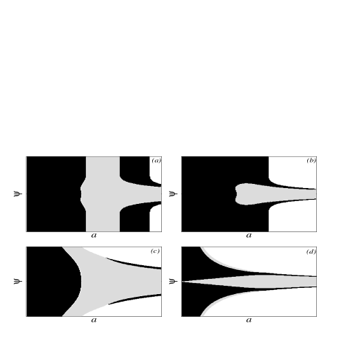
Figure 1: Regions where points of maximal expansion (gray) and minimal contraction (black) are located in configuration space $(a,\psi)$. In Fig.1(a) $\xi=\psi^{2}$, $V$ is asymptotically flat with $\Lambda<\Lambda_{0}$; in Fig.1(b) $\xi=\psi^{2}$, $V$ is asymptotically flat with $\Lambda>\Lambda_{0}$; in Fig.1(c) $\xi=\psi^{2}$, $V=m^{2}\psi^{2}/2$; in Fig.1(d) $\xi=\psi^{4}$, $V=m^{2}\psi^{2}/2$. All plots are symmetrical with respect to transition $\psi\to-\psi$.

Eq.(20) shows that the Gauss-Bonnet term does not change the configuration of the Euclidean region. From the other hand, curves separating the points of maximal expansion ($\dot{a}=0,\ddot{a}<0$) and the points of minimal contraction ($\dot{a}=0,\ddot{a}>0$) change significantly. Substituting the condition $\dot{a}=0$ into (18) and expressing $\dot{\psi}$ from (20) we obtain the following equation for the separating curve

$$-\frac{2}{a^{2}}+V(\psi)+\frac{4\delta}{a^{2}}\xi^{\prime\prime}(\psi)\biggl{(}-\frac{3}{a^{2}}+V(\psi)\biggr{)}+\frac{2\delta\xi^{\prime}(\psi)V^{\prime}(\psi)}{a^{2}}=0\mskip 5.0mu plus 5.0mu.$$ (21)

We start with the case $\xi=\psi^{2}$. As for the flat metrics, this case is exceptional one. Zero modulus potential leads to asymptotic (2) with constant scale factor $a=a_{0}=\sqrt{-12\delta}$. The separating curve is simply the line $a=a_{0}$. All the terms in constraint (20) tend to a constant value on this asymptotic and, therefore, only an asymptotically flat potentials could not destroy it. Small enough $\Lambda$ corresponds to the situation of Fig.1(a), the nonsingular regime is preserved. This picture changes if $\Lambda$ exceeds the value $\Lambda_{0}=(2+\sqrt{3})/(4|\delta|)$ (Fig.1(b)). In this case the regime $a\to a_{0}$ disappears and a trajectory which describes a contracting universe can either fall into a singularity or pass trough a bounce and enter an expanding phase. Potentials unbounded from above always violate the nonsingular asymptotic (2).

Now we consider the important case $V=m^{2}\psi^{2}/2$ in a more detail (Fig.1(c)).

The equations (18)-(20) were solved numerically using the method of integration over an additional parameter developed in Ref. [6]. The maximal expansion point was chosen as an initial data for the Cauchi problem, unknown values were obtained from the constraint equation (20).

If we start from the point with $\dot{a}=0$, initial data corresponding to solutions experiencing at least one bounce forms the system of quasiparallel zones in the initial condition space ($a,\psi$). This system is rather similar to those studied recently in the closed FRW models without the Gauss-Bonnet term [13], but has several important new features.

Figure 2: The $\psi=0$ cross-sections of zones in initial condition space $(a,\psi)$ leading to bounce for $V=m^{2}\psi^{2}/2$. In Fig.2(a) $\xi=\psi^{2}$, in Fig2(b) $\xi=cosh(\psi)$

First of all, it is clear from the separating curve configuration that if the initial scale factor is less than $\sqrt{-12\delta}$, the trajectory starts from the bounce itself. So, the 1-st bounce interval is adjacent to the axis $a=0$ in contrast to the results of Ref.[13]. Another important feature can be seen from the Fig.2(a). We plotted cross-sections $\psi=0$ of the bounce intervals depending on the mass $m$. If $m<0.6$ we can see the full set of intervals: trajectories from 1-st interval have a bounce with no $\psi$-turns before it, trajectories which have initial point of maximal expansion between 1-st and 2-nd intervals fall into a singularity after one $\psi$-turn, those from 2-nd interval have a bounce after 1 $\psi$-turn and so on. If $m$ becomes bigger than $0.6$, the 2-nd interval contains trajectories with 2 $\psi$-turns before bounce, the space between 1-st interval (which is now the product of two merged intervals) and the 2-nd one contains trajectories falling into a singularity after two $\psi$-turns. There are no trajectories going to a singularity with exactly one $\psi$-turn.

This process of interval merging continues with the modulus field mass $m$ increasing. The picture is similar to the case without the Gauss-Bonnet term but with gently sloping potential [15], where the process of interval merging also takes place. In both cases, the interval formed by merging contains very chaotic trajectories which can not be described in a way similar to [13]. A significant part of trajectories starting from such an interval may oscillate during very long time without falling into a singularity or leaving the interval. In Fig.3. we present the number of trajectories having at least 50 oscillations of modulus field versus the modulus field mass. The initial scale factor varies with step $0.02$ in the range of scale factors from $1$ to $5$ units (total number of trajectories for each value of modulus mass is equal to $200$). We ignore trajectories which describe a long-time expansion (the calculations stopped when running scale factor was 10 times greater than the initial one), so, all counted trajectories represented the chaotic oscillations. A special effort was done [17] to construct very chaotic solutions in a closed FRW model without the Gauss-Bonnet term, and trajectories having at most $12$ oscillations of scalar field were found. We choose a much bigger value ($50$ oscillations), so the existence of such trajectories tells us that a qualitatively more complicated chaos exists in the system (18)-(20). If $m<0.7$ the measure of such trajectories is so small, that they do not appear on our grid. For bigger $m$ this measure grows rather rapidly. For the mass exceeding the first merging value $1.3$ times more than $30\%$ of trajectories having the point of maximal expansion in $\psi=0$ cross-section of the first interval are very chaotic. So, the regime of chaotic oscillation for modulus field masses exceeding the first merging value is much more significant than for the case without the Gauss-Bonnet term.

This picture does not change qualitatively if we switch on the self-interaction of the modulus field. For the pure self-interacting potential $V(\psi)=\lambda\psi^{4}$ the corresponding critical value of $\lambda$ leading to the first bounce interval merging is equal to $\sim 1.2$.

Figure 3: The number of trajectories avoiding a singularity during first 50 oscillations of the modulus field. Total number of trajectories is equal to 200, initial scale factors are located in the range of two first bounce intervals

When $\xi(\psi)$ grows faster than $\psi^{2}$, there are no solution with asymptotically constant scale factor even with the vanishing modulus field potential. For $\xi\sim\psi^{n+1}$ the asymptotic solution is

$$a(t) = \sqrt{\frac{n+3}{2n}}(n+1)^{\frac{n-1}{n+1}}(-4n\delta)^{\frac{1}{n+1}}t^{\frac{n-1}{n+1}}\mskip 5.0mu plus 5.0mu,$$

$$\psi(t) = \left(-\frac{(n+1)^{2}}{4n\delta}\right)^{\frac{1}{n+1}}t^{\frac{2}{n+1}}\mskip 5.0mu plus 5.0mu,$$ (22)

for $\xi\sim exp(|\psi|)$ the solution was found by Easter and Maeda in [5]. In both cases it describes the universe with growing scalar factor and modulus field. The Gauss-Bonnet term tends to zero and, therefore, at some point it becomes unimportant in comparison with arbitrary non-vanishing modulus field potential. After that, the evolution of the universe obeys the well-known rules for FRW dynamics with the massive scalar field which inevitably lead to recollapse.

Now it is time to outline the bouncing properties in this case. The separating curve looks like plotted in Fig.1(d). But the $\psi=0$ cross-section of bouncing intervals is not changed much in comparison with the $\xi\sim\psi^{2}$ case. Again, there is the first interval in the range of very small scale factors, which is now becoming thinner with the growing modulus field. The merging of the bouncing intervals leading to significant chaotisation of trajectories is also takes place (Fig.2(b)).

Additionally we conclude from Fig.2(b) that though the asymptotic (22) for zero modulus potential is regular, taking into account the classical evolution of the Universe trough the maximal expansion point back to the large curvature regime makes the dynamics chaotic with the strong dependence on the initial condition. Similar to the $\xi=\psi^{2}$ case we have no regular nonsingular solutions, but there are infinite number of unstable chaotic trajectories escaping a singularity for an arbitrary long time.

4 Conclusions

In this paper we investigated the cosmological behavior of the model with the second order curvature corrections based on the action (3) for flat and closed FRW metrics. A particular attention was paid to the possibility of nonsingular past asymptotics. We confirm recent claims [10, 11, 12] that such regimes exist at least for functions $\xi(\psi)$ with $\xi^{\prime\prime}>0$ and present corresponding formulas for power-law and exponentially steep $\xi(\psi)$. The previously known case $\xi\sim\psi^{2}$ appears to be in some sense the exceptional one. It corresponds to DeSitter flat universe or closed universe with the constant scale factor (see Eqs.(2),(8)). Steeper $\xi(\psi)$ lead to power-low dependence of the Hubble parameter upon time for the flat metric and to bounce nonsingular solutions for the closed one (a particular example with exponentially steep $\xi(\psi)$ for the latter case was also studied by Easther and Maeda in [5]). The important point also mentioned in above cited papers is that these asymptotic regimes do not require a fine-tuning of initial conditions.

This optimistic view on the nonsingular regimes changes, however, if we take into account possible potential term for modulus field, which naturally arises in the description of SUSY breaking. We conclude that a modulus potential destroys the nonsingular asymptotics in most cases we have studied. For a flat universe the only case with $\xi^{\prime\prime}>0$ which allows nonsingular regime and a massive modulus field is $\xi\sim\psi^{2}$. Even in this case a steeper modulus potential kills the nonsingular asymptotic. For $\xi\sim\psi^{4}$ it can survive only for asymptotically flat potentials. Steeper $\xi$ can not prevent from falling into a singularity with an arbitrary modulus field potential not tending to zero for $|\psi|\to\infty$. Our numerical simulations show that when the nonsingular regime described above becomes impossible, all the cosmological trajectories go towards a singularity and no new nonsingular regime appear.

For a closed universe the possibility of regular nonsingular asymptotic is even more restricted. The above mentioned asymptotic can survive only in the exceptional case $\xi\sim\psi^{2}$ and an asymptotically flat potential. But now a trajectory which does not belong to this regime may either fall into a singularity or experience bounce, depending on the initial conditions. At the expanding phase after bounce the Gauss-Bonnet term become irrelevant and we can use the results obtained for the scalar field in Einstein theory. Since for the closed metric all the trajectories must have their point of maximal expansion, a bouncing universe will begin to contract at some point and, at the second time, fall into a singularity or have a second bounce etc. So, we return to the chaotic picture similar to one described for the massive scalar field coupled with the Einstein gravity. This chaotic regime is very sensitive to the initial condition and does not contain any stable nonsingular trajectory.

For steeper $\xi(\psi)$ the regime without a modulus potential is a bounce itself, so arbitrary potential at the after-bounce stage will dominate the Gauss-Bonnet term and lead to recollapse and chaotisation of trajectories.

Since the particular form of second order curvature corrections arising from the string theory include exponentially steep $\xi(\psi)$ with coming from SUSY breaking exponentially steep modulus potential, nonsingular solutions presenting in the string gravity with $V(\psi)=0$ disappear when modulus potential is taken into account.

Acknowlegements

This work was partially supported by Russian Foundation for Basic Research via grant N 99-02-16224. A.T. is grateful to T.Damour for useful discussion.

References

References

- [1] M.B.Green, J.H. Schwartz and E.Witten, “Superstring Theory”, Cambridge University Press, Cambridge (1986).
- [2] J.H. Schwarz, Phys. Rep. 315, 107 (1999).
- [3] S. Mignemi and N.R. Stewart, Phys. Rev. D 47, 5259 (1993);
- [4] P. Kanti, N.E. Mavromatos, J. Rizos, K. Tamvakis and E. Winstanley, Phys. Rev. D 54, 5049 (1996); P. Kanti and K. Tamvakis, Phys. Lett. B 392, 30 (1997).
- [5] R. Easter and K. Maeda, Phys. Rev. D 54, 7252 (1996).
- [6] S.O. Alexeyev and M.V. Pomazanov, Phys. Rev. D 55, 2110 (1997); S.O. Alexeyev and M.V. Sazhin, Gen. Relativ. and Grav. 8, 1187-1203 (1998).
- [7] T. Torii, H. Yajima and K. Maeda, Phys. Rev. D 55, 739 (1997); R.C. Myers, “Black Holes in Higher Curvature Gravity”, in “Black Holes, Gravitational Radiation and the Universe: Essays in Honor of C.V. Vishveshwara”, eds C.V. Vishveshwara, B.R.Iyer, B.Brawal, gr-qc/9811042.
- [8] T. Banks, Nucl. Phys. Proc. Suppl. 67, 180 (1998); J.H. Schwarz and N.Seiberg, Rev. Mod. Phys. 71, S112 (1999).
- [9] T.Jacobson, “Black Hole Thermodynamics Today”, Talk, given at 8th Marcel Grossman Meeting on Recent Developments in Theoretical and Experimental General Relativity, Gravitation and Relativistic Theories (MG8), Jerusalem, Israel, 22-27 June 1997, gr-qc/9801015.
- [10] I. Antoniadis, J. Rizos and K. Tamvakis, Nucl. Phys. B415 497 (1994).
- [11] J. Rizos and K. Tamvakis, Phys. Lett. B326, 57 (1994).
- [12] P. Kanti, J. Rizos and K. Tamvakis, Phys. Rev. D59, 083512 (1999).
- [13] A.Yu.Kamenshchik, I.M.Khalatnikov, A.V.Toporensky, Int. J. Mod. Phys. D6, 673 (1997).
- [14] A.Tseytlin, “String Solutions with Nonconstant Scalar Fields” Published in the proceedings of International Symposium on Particle Theory, Wendisch-Rietz, Germany, 7-11 Sep 1993 (Ahrenshoop Symp.1993:0001-13), hep-th/9402082
- [15] S.A.Pavluchenko and A.V.Toporensky, “Chaos in FRW Cosmology with Gently Sloping Scalar Field Potentials”, gr-qc/9911039.
- [16] S. Foster, “Scalar Field Cosmological Models With Hard Potential Walls,” gr-qc/9806113.
- [17] N.J. Cornish, E.P.S. Shellard, Phys. Rev. Lett. 81, 3571 (1998).