Recent developments in quantum string cosmology

Abstract

In this talk we discuss the quantisation of a class of string cosmology models characterised by scale factor duality invariance. The amplitudes for the full set of classically allowed and forbidden transitions are computed by applying the reduced phase space and path integral methods. In particular, the path integral calculation clarifies the meaning of the instanton-like behaviour of the transition amplitudes that has been first pointed out in previous investigations.

1 Introduction

One of the main problems of ‘pre-big bang’ string cosmology [1, 2, 3] is the understanding of the mechanism responsible for the transition (‘graceful exit’) from the inflationary ‘pre-big bang’ (PRBB) phase to a deflationary ‘post-big bang’ phase (POBB) with decreasing curvature typical of the standard cosmological scenario. Necessarily, the graceful exit involves a high-curvature, strong coupling, regime where higher derivatives and string loops terms must be taken into account. It has been shown [4] that for any choice of the (local) dilaton potential no cosmological solutions that connect smoothly the PRBB and POBB phases do exist. As a consequence, at the classical level higher order corrections cannot be ‘simulated’ by any realistic dilaton potential.

At the quantum level the dilaton potential may induce the transition from the PRBB phase to the POBB phase. In this context, using the standard Dirac method of quantisation based on the Wheeler-De Witt equation, a number of minisuperspace models have been investigated in the literature [5, 6, 7]. The result of these investigations is a finite, non-zero, transition probability PRBB $\rightarrow$ POBB with a typical ‘instanton-like’ dependence ($\sim\,\exp\{-1/g^{2}\}$) on the string coupling constant.

In this talk we present a refined analysis of the quantisation of string cosmological models by reconsidering the minisuperspace models previously investigated [5, 6, 7]. We will consider a class of string inspired models that are exactly integrable and apply the standard techniques for the canonical quantisation of constrained systems.

2 Classical theory

We consider the string inspired model in d+1 dimensions described by the action

$$S=\int\,\frac{d^{{\rm d}+1}x}{2\lambda_{s}^{{\rm d}-1}}\,\sqrt{|g|}\,e^{-\phi}\,\left(R+\partial_{\mu}\phi\partial^{\mu}\phi-V\right),$$ (2.1)

where $\phi$ is the dilaton field, $\lambda_{s}=(\alpha^{\prime})^{1/2}$ is the fundamental string length parameter, and $V=V(g_{\mu\nu},\phi)$ is a potential term. We deal with isotropic, spatially flat, cosmological backgrounds with finite volume spatial sections. For this class of backgrounds the action (2.1) reads

$$S=\int\,dt\,{\lambda_{s}\over 2}\,\left({1\over\mu}(\dot{\Theta}^{2}-\dot{\Phi}^{2})-\mu\,e^{-2\Phi}V\right)\,,$$ (2.2)

where we have used the metric parametrisation $g_{\mu\nu}={\rm diag}\left(-\mu^{2}(t)e^{-2\Phi},a^{2}(t)\delta_{ij}\right)$, $i,j=1,..$d, $a=\exp[\Theta(t)/\sqrt{{\rm d}}]$. $\Phi=\phi-\log\,\int\,d^{\rm d}x/\lambda_{s}^{\rm d}-\sqrt{{\rm d}}\,\Theta$ is the ‘shifted’ dilaton field. We shall restrict our attention to models which exhibit scale factor duality invariance [1] (in this case the potential term depends only on the shifted dilaton $\Phi$). Moreover, we shall consider potentials of the form $V(\Phi)=\lambda\,e^{-2\Phi(q-1)}$, where $\lambda>0$ is a dimension-two quantity (in natural units) and $q$ is a dimensionless parameter. (This class of potentials has been first discussed in [7].) It is also convenient to use the canonical form for the action

$$S=\int dt\,\left[\dot{\Theta}\Pi_{\Theta}+\dot{\Phi}\Pi_{\Phi}-{\cal H}\right]\,,{\cal H}=\mu(t)H\,,$$ (2.3)

where the Hamiltonian constraint $H$ reads

$$H={1\over 2\lambda_{s}}\left(\Pi_{\Theta}^{2}-\Pi_{\Phi}^{2}+\lambda_{s}^{2}V(\Phi)\,e^{-2\Phi}\right)\,.$$ (2.4)

For $q\neq 0$ the explicit solution of the equations of motion has been derived and discussed in [9]. The expanding and contracting backgrounds are identified by the value $\Pi_{\Theta}=k>0$ and $\Pi_{\Theta}=k<0$, respectively ($k=0$ corresponds to the flat (d+1)-dimensional Minkowski space). Moreover, for $q\leq 1$ we have two distinct branches corresponding to PRBB $(+)$ and POBB $(-)$ states, that are identified by negative and positive values of $\Pi_{\Phi}$, respectively.

3 Quantum theory

The class of models introduced in the previous section is described by a time-reparametrisation invariant Hamiltonian system with two degrees of freedom. Thanks to the integrability properties of this class of models, the standard techniques of quantisation of constrained systems can be applied straightforwardly. In particular, since the constraint $H$ is of the form $H=H_{\Theta}(\Theta)+H_{\Phi}(\Phi)$ the time parameter can be defined by a single degree of freedom. Since we are interested in the calculation of the quantum transition probability from a (expanding) PRBB phase to a (expanding) POBB phase, it is natural to use the $(\Theta,\Pi_{\Theta})$ degree of freedom to define the time of the system and fix the gauge. In this case the eigenstates of the effective Hamiltonian are identified by a continuous quantum number $k$ corresponding to the classical value of $\Pi_{\Theta}$. Wave functions that describe expanding (contracting) solutions are eigenstates of the effective Hamiltonian with $k>0$ ($k<0$).

Let us perform the canonical transformation $\Sigma=\lambda_{s}\Theta/\Pi_{\Theta}$, $\Pi_{\Sigma}=\Pi_{\Theta}^{2}/2\lambda_{s}$ [8]. Since $\Sigma$ is canonically conjugate to $H$ it defines a global time parameter. Thus the gauge fixing identity can be chosen as $F(\Sigma;t)\equiv\Sigma+t=0$, fixing the Lagrange multiplier as $\mu=-1$. The gauge-fixed action reads

$$S_{\rm eff}=\int_{t_{1}}^{t_{2}}dt\,\left[\dot{\Phi}\,\Pi_{\Phi}\,-\,H_{\rm eff}(\Phi,\Pi_{\Phi})\right]\,,$$ (3.1)

where the effective Hamiltonian is

$$H_{\rm eff}(\Phi,\Pi_{\Phi})={1\over 2\lambda_{s}}\left(\Pi_{\Phi}^{2}-\lambda\lambda_{s}^{2}e^{-2q\Phi}\right)\,.$$ (3.2)

The system described by the effective Hamiltonian (3.2) is free of gauge degrees of freedom and its quantisation can be performed using the standard techniques. We shall now discuss the reduced phase space and path integral quantisation procedures.

3.1 Reduced phase space quantisation

The reduced phase space is described by a single degree of freedom with canonical coordinates $(\Phi\in{\vrule height=6.88889pt,width=0.50003pt,depth=0.0pt\kern-0.59998pt{\rm R}},\Pi_{\Phi}\in{\vrule height=6.88889pt,width=0.50003pt,depth=0.0pt\kern-0.59998pt{\rm R}})$. The Schrödinger equation reads

$$-i{\partial~{}\over\partial t}\,\Psi=\,{1\over 2\lambda_{s}}\left[{\partial^{2}~{}\over\partial\Phi^{2}}+\lambda\lambda_{s}^{2}e^{-2q\Phi}\right]\,\Psi\,.$$ (3.3)

The general solution of (3.3) can be written in terms of the solutions $\psi_{k,q}(\Phi)$ of the stationary Schrödinger equation $\hat{H}_{\rm eff}\psi=E\psi$ with energy $E=k^{2}/2\lambda_{s}$

$$\psi_{k,q}(z)=A_{1}(k,q)J_{i\nu}(z)+A_{2}(k,q)Y_{i\nu}(z)\,,$$ (3.4)

where $J_{i\nu}(z)$ and $Y_{i\nu}(z)$ are the Bessel functions of the first and second kind of index $i\nu=i|k/q|$ and argument $z=\sqrt{\lambda}\lambda_{s}\exp(-q\Phi)/|q|$. In particular, two sets of orthonormal stationary solutions can be chosen as the stationary wave functions corresponding to expanding PRBB and POBB phases, either in perturbative regime or in the strong coupling regime. For $q>0$, the normalised PRBB(+) and POBB (-) wave functions in the weak coupling (W) and strong coupling (S) regimes are

$$\psi^{\rm(\pm)}_{W}={1\over\sqrt{2\hbox{\rm coth}(\pi\nu)}}\left[\sqrt{\hbox{\rm tanh}(\pi\nu/2)}\chi^{(1)}_{\nu}\mp\right.$$

$$\left.i\sqrt{\hbox{\rm coth}(\pi\nu/2)}\chi^{(2)}_{\nu}\right]\,,$$ (3.5)

$$\psi^{\rm(\pm)}_{S}={1\over\sqrt{2}}\left[\chi^{(1)}_{\nu}\mp i\chi^{(2)}_{\nu}\right]\,,$$ (3.6)

where $\chi^{(1)}_{\nu}(z)$ and $\chi^{(2)}_{\nu}(z)$ are linear combinations of the Hankel functions $H^{(1,2)}_{i\nu}(z)$. Using the two sets of wave functions (3.5) and (3.6) it is possible to compute the amplitudes that correspond to different transitions (a detailed analysis of those amplitudes can be found in [9]). In particular, the transition probabilities that correspond to classically allowed transitions read

$$P_{S,W}^{(+,+)}=P_{S,W}^{(-,-)}={1\over 1+e^{-2\pi k/q}}\,.$$ (3.7)

Transitions between PRBB weak (strong) coupling regime and POBB strong (weak) coupling regime are classically forbidden; the relative transition probabilities are given by

$$P_{W,S}^{(+,-)}=P_{S,W}^{(+,-)}={e^{-2\pi k/q}\over 1+e^{-2\pi k/q}}\,.$$ (3.8)

The last and most interesting result is the probability of transition from the PRBB phase in the weak coupling regime to the POBB phase in the weak coupling regime

$$P_{W,W}^{(+,-)}=4{e^{-2\pi k/q}\over\left(1+e^{-2\pi k/q}\right)^{2}}\,.$$ (3.9)

For $q=1$, the semiclassical limit ($k\gg 1$) of (3.9) coincides, apart from a normalisation factor, with the ‘reflection-coefficient’ of [5, 6]. However, the result of [5, 6] should be considered as a ratio between two different transition probabilities rather than a transition probability by itself. Precisely, the reflection-coefficient defined in [5, 6] is $R\equiv P_{S,W}^{(-,+)}/P_{S,W}^{(+,+)}=e^{-2\pi k/q}$.

These results show that the probabilities of classically forbidden transitions can be expressed, in the semiclassical limit, as power series of $e^{-2\pi k/|q|}$. Following [5, 6], we find

$$\exp(-2\pi k/|q|)=\exp\left(-\sqrt{4d}\,\pi\Omega_{s}\over|q|g^{2}_{s}\,\lambda^{d}_{s}\right)\,,$$ (3.10)

where $\Omega_{s}$ is the proper spatial volume and $g_{s}=e^{\phi_{s}/2}$ is the value of the string coupling when the Hubble parameter is equal to $1/\lambda_{s}$. The ‘istanton-like’ behaviour of (3.10) shows that the probabilities of classically forbidden transitions are peaked in the strong coupling regime – as it was first pointed out in [5, 6] – where all powers of $e^{-2\pi k/|q|}$ have to be taken into account. The occurrence of this istanton-like behaviour will be discussed in the next subsection.

3.2 Path integral quantisation

The string cosmology model that we are considering can also be quantised using the functional approach. Applying the path integral formalism, we compute the probability $P_{W,W}^{(+,-)}=|A_{W,W}^{(+,-)}|^{2}$ in the semiclassical limit [9]. The starting point of the functional approach is the path integral in the reduced space

$$I=\int_{\Phi(t_{1})}^{\Phi(t_{2})}\,{\cal D}\Phi\,\exp\left(i\int_{t_{1}}^{t_{2}}dt\,{\cal L}_{\rm eff}[\Phi,\dot{\Phi}]\right)\,,$$ (3.11)

where the effective Lagrangian can be obtained from the effective Hamiltonian (3.2). The transition amplitude $A_{W,W}^{(+,-)}$ is defined by (3.11) where the integral is evaluated on all paths that satisfy the boundary conditions $z(-\infty)=\infty$, $z(\infty)=\infty$. (Recall that $z=\sqrt{\lambda}\lambda_{s}\exp(-q\Phi)/|q|$.) Let us consider the analytical continuation of the variable $z$ to the complex plane. The effective Lagrangian is analytical in any point of the complex plane $({\rm Re}(z),{\rm Im}(z))$ save for $z=0$. Classically, the transition from the weak coupling PRBB phase to the weak coupling POBB phase would correspond to the trajectory starting at $z=+\infty$, going left along the real axis (PRBB phase, $\dot{\Phi}>0$), reaching the origin, and finally going right along the real axis to $z=+\infty$ (POBB phase, $\dot{\Phi}<0$). Clearly, since the Lagrangian is singular in $z=0$ a classical continuous and differentiable solution does not exist.

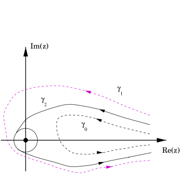
Figure 1: Contours of integration in the complex $z$-plane.

Now consider generic analytical trajectories in the complex plane that start at $Re(z)=\infty$, $Im(z)>0$, and end at $Re(z)=\infty$, $Im(z)<0$ (see Fig.1). We can divide this class of trajectories in three (topologically) distinct categories: Trajectories that do not cross the imaginary axis, (curve $\gamma_{0}$ in Fig.1); trajectories that cross twice the imaginary axis, (curve $\gamma_{1}$ in Fig. 1); trajectories that cross $2n$ times ($n=2,3...$) the imaginary axis, (curve $\gamma_{n}$ in Fig. 1 for $n=2$). It is straightforward to see that the trajectories of type $\gamma_{0}$ do not describe transitions from PRBB to POBB phases. A trajectory of type $\gamma_{1}$ describes a transition from the weak coupling PRBB phase to the weak coupling POBB phase. It can be deformed continuously into a classical solution except in a small region in the strong coupling limit, where the singularity of the classical solution is avoided by the analytical continuation in the complex plane. The path integral evaluated on this trajectory gives the leading contribution to the semiclassical approximation of the transition amplitude $A_{W,W}^{(+,-)}$. Trajectories of type $\gamma_{n}$ (with $n\,>\,1$) give contributes of higher order. In particular, any trajectory that circles $z=0$ can be considered as an ‘$n$-instanton’ solution (with no well-defined signature) labelled by a winding number $n$ that corresponds to the number of times that the trajectory wraps around the singularity in $z=0$. In the semiclassical limit, the transition amplitude $P_{W,W}^{(+,-)}$ is given by the path integral (3.11) evaluated on the class of $n$-instanton solutions. For the class of 1-instanton trajectories the amplitude is given by

$$A_{W,W}^{(+,-)(1)}=C_{1}e^{-\pi k/q}\,,$$ (3.12)

where $C_{1}$ is a normalisation factor. The square of the semiclassical one-instanton amplitude (3.12) approximates the (exact) result (3.9) for large values of $k$. This proves the consistency of the reduced phase space and path integral quantisation methods. The contribution of the $n$-instanton ($n\,>\,1$) to the transition amplitude $A_{W,W}^{(+,-)}$ is

$$A_{W,W}^{(+,-)(n)}=C_{n}e^{-\pi nk/q}\,.$$ (3.13)

Hence, $n$-instanton terms give higher order contributions in the large-$k$ expansion. Equations (3.12) and (3.13) show that the instanton-like dependence (3.10) of the amplitudes that correspond to classically forbidden transitions can be traced back to the existence, in the semiclassical regime, of trajectories that connect smoothly the PRBB and POBB phases.

References

- [1] G. Veneziano, Phys. Lett B265 (1991) 387.
- [2] M. Gasperini and G. Veneziano, Astropart. Journal 1 (993) 317;
- [3] M. Gasperini and G. Veneziano, Mod. Phys. Lett. A83 (113) 701; Phys. Rev. D50 (1994) 2519.
- [4] R. Brustein and G. Veneziano, Phys. Lett. B329 (1994) 429; N. Kaloper, R. Madden and K.A. Olive, Nucl. Phys. B452 (1995) 677; Phys. Lett B371 (1996) 34; R. Easther, K. Maeda and D. Wands, Phys. Rev. D53 (1996) 4247.
- [5] M. Gasperini and G. Veneziano, Gen. Rel. Grav. 28 (1996) 1301.
- [6] M. Gasperini, J. Maharana and G. Veneziano, Nucl. Phys. B472 (1996) 349.
- [7] J. Maharana, S. Mukherji and S. Panda, Mod. Phys.Lett. A12 (1997) 447.
- [8] M. Cavaglià and V. de Alfaro, Gen. Rel. Grav. 29 (1997) 773.
- [9] M. Cavaglià and C. Ungarelli, Class. and Quant. Grav 16 (1999) 1401.