Phys. Rev. D 62, 104006 (2000)
Cauchy boundaries in linearized gravitational theory

Abstract

We investigate the numerical stability of Cauchy evolution of linearized gravitational theory in a 3-dimensional bounded domain. Criteria of robust stability are proposed, developed into a testbed and used to study various evolution-boundary algorithms. We construct a standard explicit finite difference code which solves the unconstrained linearized Einstein equations in the $3+1$ formulation and measure its stability properties under Dirichlet, Neumann and Sommerfeld boundary conditions. We demonstrate the robust stability of a specific evolution-boundary algorithm under random constraint violating initial data and random boundary data.

I Introduction

The computational evolution of 3-dimensional general relativistic space-times by means of Cauchy evolution is a potentially powerful tool to study the gravitational radiation from black-hole/neutron-star binaries whose inspiral are expected to provide prominent signals to gravitational wave observatories. There are several 3-dimensional general relativistic codes under development to solve this problem. Boundary conditions are an essential part of these codes. At the outer boundary they must provide an outgoing radiation condition and extract the emitted waveform. For black-hole spacetimes, there is also an inner boundary, approximately given by the apparent horizon, where one excises the singular region inside a black hole. Instabilities or inaccuracies introduced at such boundaries have emerged as a major problem common to all code development. Historically, the first Cauchy codes were based upon the Arnowitt-Deser-Misner (ADM) formulation [1, 2] of the Einstein equations. Recently there has been pessimism that such codes might be inherently unstable because of the lack of manifest hyperbolicity in the underlying equations. In order to shed light on this issue, we present here a study of ADM evolution-boundary algorithms in the simple environment of linearized gravity, where nonlinear sources of physical or numerical instability are absent and computing time is reduced by a factor of five by use of a linearized code.

Our two main results, for the case of fixed lapse and shift, are:

• On analytic grounds, ADM boundary algorithms which supply values for all components of the metric (or extrinsic curvature) are inconsistent.

• We present a boundary algorithm which allows free specification of the transverse-traceless components of the metric (or extrinsic curvature) at the boundary, and for which unconstrained, linearized ADM evolution can be carried out in a bounded domain for thousands of crossing times with robust stability.

The criteria for robust stability, which we present here, are the most severe that have been applied to Cauchy evolution in numerical relativity. The boundary algorithm differs from previous approaches and offers fresh hope for robust nonlinear ADM evolution.

Our particular motivation for this work is the difficulty we have experienced implementing Cauchy-characteristic-matching (CCM) for 3-dimensional general relativity [3, 4]. CCM provides a Cauchy boundary condition by matching the Cauchy evolution across the boundary to a characteristic evolution. For nonlinear scalar waves propagating in a flat 3-dimensional space, CCM has been demonstrated to be more accurate and efficient than all other existing boundary conditions for Cauchy evolution [5], and it has been demonstrated mathematically that this conclusion also applies to gravity [6]. In addition, in the spherically symmetric case of a self gravitating scalar wave satisfying the Einstein-Klein-Gordon equations, CCM has been successfully applied at the inner boundary of a Cauchy evolution to excise the interior black hole region and, at the same time, at the outer boundary to provide a global evolution on a compactified grid extending to null infinity [7]. These successes are promising for the application of CCM to 3-dimensional problems in general relativity but this has not yet been borne out. This difficulty, and the similar difficulty in efforts using perturbative matching [8], may possibly arise from a pathology of the Cauchy boundary which is independent of matching. In this work, we reveal such a pathology in the way boundary conditions have been applied in the ADM formulation of the Einstein equations which, at present, is the only formulation for which matching has been attempted. We also present a new form of ADM boundary algorithm which eliminates the pathology.

The stability of the Cauchy evolution algorithm itself is straightforward to investigate by carrying out a boundary-free evolution on a 3-torus (equivalent to periodic boundary conditions). Such tests constitute Stage 1 of a 3-stage test bed for robust boundary stability which is summarized below and explained in detail in Sections III, IV and  VI. The periodic boundary tests serve to cull out algorithms whose boundary stability is doomed from the start. In earlier work, robust stability for characteristic evolution with random data on an inner boundary was demonstrated for characteristic evolution using the PITT Null Code [6]. In the course of the present investigation we have reconfirmed this robustness of the PITT code using the same specifications proposed here for Cauchy codes.

CCM cannot work unless the Cauchy code, as well as the characteristic code, has a robustly stable boundary. This is necessarily so because the interpolations between a Cartesian Cauchy grid and a spherical null grid continually introduce short wavelength noise into the neighborhood of the boundary. This is the rationale underlying the robustness criterion in our test bed. Robustness of the Cauchy boundary is a necessary (although not a sufficient) condition for the successful implementation of CCM.

Analytic studies of Cauchy evolution of linearized gravity with boundaries at infinity reveal modes which grow linearly in time, but none which grow exponentially [9]. The inaccuracy introduced by such secular modes can be controlled and is not of major concern, at least in the linearized theory. (Such secular modes can lead to exponential instabilities of numerical origin in the nonlinear theory if not properly treated [10]). In the case of a finite boundary, there is further potential for instability and a brief discussion is given in Sec. III.

As is customary in numerical relativity, we monitor the existence of unstable modes by the growth of the Hamiltonian constraint. Because the constraints are not enforced during standard implementation of ADM evolution, the Hamiltonian constraint is an effective sensor of numerical instabilities.

Stage 2 of the test bed is based on the simple boundary value problem obtained by opening one dimension of a 3-torus to form a 2-torus with plane boundaries normal to a Cartesian axis. Running a Cauchy-boundary algorithm with this topology and with random initial and random boundary data forms the second stage of our test bed, which is discussed in Sec. IV. In Sec. V, we present new evolution-boundary algorithms which are robustly stable.

Stage 3 of the testbed is designed to test robustness of boundary conditions appropriate to an isolated system. In Sec. VI we establish Stage 3 robustness of an ADM boundary algorithm.

The main results presented here are experimental, in a computational sense. The difficulties encountered with finite Cauchy boundaries in general relativity have recently prompted some analytic investigations of the subject [11, 12]. However, these have so far been confined to hyperbolic formulations, as opposed to the ADM formulation, and to the analytic problem, as opposed to the finite difference solution obtained by computation. Although it is not possible to make a direct comparison, the nature of our results are consistent with the general conclusions of these analytic studies.

There are several promising numerical approaches based upon hyperbolic (or “more hyperbolic”) formulations of the equations [13, 14, 15, 16, 17, 18, 19, 20, 21, 22, 23]. Here we concentrate on ADM schemes, which are the most compact to code and require the least amount of memory because they have a smaller number of variables. Our results should provide useful benchmarks for other relativity codes. However, it should also be cautioned that the nature of a successful boundary algorithm is dependent on the form of the equations adopted, as well as the choice of discretization, and the ADM boundary algorithms we have obtained do not necessarily apply to other formulations.

We use Greek letters for space-time indices and Latin letters for spatial indices. Four dimensional geometric quantities are explicitly indicated, such as ${}^{(4)}R_{\alpha\beta}$ and ${}^{(4)}G_{\alpha\beta}$ for the Ricci and Einstein tensors of the space-time, whereas $R_{ij}$ and $R$ refer to the Ricci tensor and Ricci scalar of the Cauchy hypersurfaces. Linearized versions of these quantities are denoted by ${}^{(4)}\tilde{R}_{\alpha\beta}$, $\tilde{R}_{ij}$, etc. Three dimensional tensor indices are raised and lowered by the background Euclidean metric $\delta_{ij}$. We write $h=\delta^{ij}h_{ij}$ for 3-dimensional traces. We denote time derivatives by $\dot{f}=\partial_{t}f$. Our convention for the background Minkowski metric is such that the wave equation takes the form

$$\eta^{\alpha\beta}\partial_{\alpha}\partial_{\beta}\Phi=(-\partial_{t}^{2}+\partial_{x}^{2}+\partial_{y}^{2}+\partial_{z}^{2})\Phi=0.$$ (1)

II General Framework

A The linearized ADM system

The ADM formulation of the Einstein equations introduces a foliation of space-time by a time coordinate $t$ and expresses the 4-dimensional metric as

$$ds^{2}=-\alpha^{2}dt^{2}+g_{ij}\left(dx^{i}+\beta^{i}dt\right)\left(dx^{j}+\beta^{j}dt\right),$$ (2)

where $g_{ij}$ is the induced 3-metric of the $t=const$ slices, $\alpha$ is the lapse and $\beta^{i}$ the shift, with the normal to the slices given by $n^{\mu}=(1,-\beta^{i})/\alpha$. The equations ${}^{(4)}R_{ij}=0$ yield the evolution equations

$$\partial_{t}g_{ij}-\pounds_{\beta}g_{ij} = -2\alpha K_{ij}$$ (3)

$$\partial_{t}K_{ij}-\pounds_{\beta}K_{ij} = -D_{i}D_{j}\alpha+\alpha\left(R_{ij}+KK_{ij}-2K_{i}^{l}K_{lj}\right),$$ (4)

for the 3-metric $g_{ij}$ and the extrinsic curvature $K_{ij}=-\frac{1}{2}\pounds_{n}g_{ij}$, subject to the constraints

$$R-K_{ij}K^{ij}+K^{2} = 0$$ (5)

$$D_{j}\left(K^{ij}-g^{ij}K\right) = 0.$$ (6)

Here $R$, $R_{ij}$ and $D_{i}$ are the Ricci scalar, Ricci tensor and connection of the 3-metric, respectively.

For simplicity we consider a gauge in which the lapse is unity and the shift vanishes (Gaussian coordinates), so that the linearized metric $g_{\alpha\beta}=\eta_{\alpha\beta}+h_{\alpha\beta}$ satisfies $h_{t\alpha}=0$, and obeys the linearized ADM evolution equations

$$\partial_{t}h_{ij} = -2K_{ij}$$ (7)

$$\partial_{t}K_{ij} = \tilde{R}_{ij},$$ (8)

subject to the (linearized) constraints

$$\tilde{R} = 0$$ (9)

$$\partial_{j}\left(K^{ij}-\delta^{ij}K\right) = 0.$$ (10)

Here we consider a 1-parameter system of equations, equivalent to the linearized Einstein equation, consisting of the six evolution equations ${\cal E}_{ij}=0$ along with the four constraint equations ${\cal C}={\cal C}_{i}=0$, where

$${\cal E}_{ij}:={}^{(4)}\tilde{R}_{ij}+\frac{1}{2}\lambda\delta_{ij}{\cal C},$$ (11)

${\cal C}:={}^{(4)}\tilde{G}_{tt}$, ${\cal C}_{i}:=-{}^{(4)}\tilde{G}_{ti}$ and the parameter $\lambda$ allows mixing the (linearized) Hamiltonian constraint ${\cal C}$ into the evolution equations. For $\lambda=0$ we recover the standard ADM system.

Codes under development for the evolution of 3-dimensional space-times without symmetry apply the constraint equations at the initial time but do not enforce them during the evolution. It is crucial for this approach that the constraints be stably propagated in time. An investigation by Frittelli [24] shows that this requires the parameter $\lambda$ in Eq. (11) satisfy $1+\lambda\geq 0$. This follows from an analysis of the linearized Bianchi identities $\partial_{\beta}{}^{(4)}\tilde{G}_{\alpha}^{\beta}\equiv 0$, which imply that

$$\dot{\cal C}^{i}+(1+\lambda)\,\partial^{i}{\cal C}+\partial_{j}{\cal E}^{ij}\equiv 0$$ (12)

$$\dot{\cal C}+\partial_{i}{\cal C}^{i}\equiv 0.$$ (13)

Thus if the evolution equations are satisfied then the Hamiltonian constraint satisfies

$$\ddot{\cal C}-(1+\lambda)\partial^{k}\partial_{k}{\cal C}=0;$$ (14)

This equation has a well-posed initial value problem for $\lambda>-1$ (when it is hyperbolic) and also for $\lambda=-1$, but for $\lambda<-1$ the equation is elliptic and the initial value problem is not well-posed. In the standard ADM case, $\lambda=0$ and the Hamiltonian constraint propagates along the light cone. We consider here evolution equations with a range of $\lambda$.

The linearized evolution equations (11) take the form

$$\dot{h}_{ij} = -2K_{ij}$$ (15)

$$\dot{K}_{ij} = -\frac{1}{2}\partial_{m}\partial^{m}h_{ij}+\frac{1}{2}(\partial_{i}H_{j}+\partial_{j}H_{i})+\frac{1}{2}\delta_{ij}\lambda{\cal C},$$ (16)

where

$$H_{i}=\partial^{j}(h_{ij}-\frac{1}{2}\delta_{ij}h).$$ (17)

and we can express the Hamiltonian as

$${\cal C}=\frac{1}{2}\partial_{i}H^{i}-\frac{1}{4}\partial_{m}\partial^{m}h.$$ (18)

A spectral analysis of a system similar to Eq’s (16) - (17) is presented in [25].

B Finite difference algorithms

The evolution variables consist of the 3-metric perturbations $h_{ij}$ and their associated momentum $K_{ij}=-\dot{h}_{ij}/2$. The evolution is implemented on a uniform spatial grid $(x_{j},y_{k},z_{l})=(j\Delta x,k\Delta x,l\Delta x)$ with time levels $t^{n}=n\Delta t$. The three different evolution algorithms we apply can be discussed in reference to the scalar wave Eq. (1), rewritten in the form

$$\dot{\Phi} = -2K$$ (19)

$$\dot{K} = -\frac{1}{2}\partial_{m}\partial^{m}\Phi,$$ (20)

analogous to the first differential order in time and second differential order in space form of the ADM equations. We denote $\Phi^{n}_{j,k,l}=\Phi(t^{n},j\Delta x,k\Delta x,l\Delta x)$. All second derivatives on the right hand side of Eq. (20) are calculated as centered 3-point finite differences.

1 Standard leapfrog (LF1)

The first evolution algorithm, which we refer to as LF1, is a standard leapfrog implementation of Eq. (20):

$$\Phi^{n+1}_{j,k,l} = \Phi^{n-1}_{j,k,l}-4K^{n}_{j,k,l}\Delta t$$ (21)

$$K^{n+1}_{j,k,l} = K^{n-1}_{j,k,l}-\nabla^{2}\Phi^{n}_{j,k,l}\Delta t,$$ (22)

where $\nabla^{2}$ is the second order accurate centered difference approximation to the Laplacian. It is known that this algorithm has a time-splitting instability in the presence of dissipative and nonlinear effects [26].

2 Staggered leapfrog (LF2)

The second evolution algorithm, which we refer to as LF2, is a staggered in time leapfrog scheme which is not subject to the time-splitting instability:

$$\Phi^{n+1}_{j,k,l} = \Phi^{n}_{j,k,l}-2K^{n+\frac{1}{2}}_{j,k,l}\Delta t$$ (23)

$$K^{n+\frac{1}{2}}_{j,k,l} = K^{n-\frac{1}{2}}_{j,k,l}-\frac{1}{2}\nabla^{2}\Phi^{n}_{j,k,l}\Delta t.$$ (24)

Here $K$ is evaluated on the half grid. Subtraction of the equation

$$\Phi^{n}_{j,k,l}=\Phi^{n-1}_{j,k,l}-2K^{n-\frac{1}{2}}_{j,k,l}\Delta t$$ (25)

from Eq. (23) and elimination of $K$ using Eq. (24) shows that LF2 is equivalent to the standard centered second-order scheme for the second differential order in time form of the wave equation (1), in which $\Phi$ lies on integral time levels and $K$ is not introduced.

3 Iterative Crank-Nicholson (ICN)

The third evolution algorithm, which we refer to as ICN, is a two-iteration Crank-Nicholson algorithm. For an $N$-iteration Crank-Nicholson algorithm, the following sequence of operations is executed at each time-step:

1. Compute the first order accurate quantities

   $$\stackrel{{\scriptstyle(0)}}{{\Phi}}\!{}^{n+1}_{j,k,l} = \Phi^{n}_{j,k,l}-2K^{n}_{j,k,l}\Delta t$$ (26)

   $$\stackrel{{\scriptstyle(0)}}{{K}}\!{}^{n+1}_{j,k,l} = K^{n}_{j,k,l}-\frac{1}{2}\nabla^{2}\Phi^{n}_{j,k,l}\Delta t.$$ (27)

2. Starting with $i=0$, compute the midlevel values

   $$\stackrel{{\scriptstyle(i)}}{{\Phi}}\!{}^{n+\frac{1}{2}}_{j,k,l} = \frac{1}{2}\left\{\Phi^{n}_{j,k,l}+\stackrel{{\scriptstyle(i)}}{{\Phi}}\!{}^{n+1}_{j,k,l}\right\}$$ (28)

   $$\stackrel{{\scriptstyle(i)}}{{K}}\!{}^{n+\frac{1}{2}}_{j,k,l} = \frac{1}{2}\left\{K^{n}_{j,k,l}+\stackrel{{\scriptstyle(i)}}{{K}}\!{}^{n+1}_{j,k,l}\right\}.$$ (29)

3. Update using levels $n$ and $n+\frac{1}{2}$,

   $$\stackrel{{\scriptstyle(i+1)}}{{\Phi}}\!{}^{n+1}_{j,k,l} = \Phi^{n}_{j,k,l}-2\stackrel{{\scriptstyle(i)}}{{K}}\!{}^{n+\frac{1}{2}}_{j,k,l}\Delta t$$ (30)

   $$\stackrel{{\scriptstyle(i+1)}}{{K}}\!{}^{n+1}_{j,k,l} = K^{n}_{j,k,l}-\frac{1}{2}\nabla^{2}\stackrel{{\scriptstyle(i)}}{{\Phi}}\!{}^{n+\frac{1}{2}}_{j,k,l}\Delta t.$$ (31)

4. Increment $i$ by one and return to step 2 until $i=N$ is reached.

A stability analysis by Teukolsky shows that the evolution scheme is stable for $N=2$ and $N=3$ iterations, unstable for $N=4$ and $N=5$, stable for $N=6$ and $N=7$, etc. [27].

4 The Courant-Friedrichs-Lewy condition

The stability of the three evolution algorithms requires they obey the Courant-Friedrichs-Lewy (CFL) condition that the numerical domain of dependence contain the analytic domain of dependence, a common requirement for explicit algorithms. For the staggered leapfrog (LF2) and the iterative Crank-Nicholson (ICN) algorithms, we set $\Delta t=\Delta x/4$ and for the standard leapfrog (LF1) we set $\Delta t=\Delta x/8$, in all cases slightly less than half the CFL condition for the algorithm.

5 Boundary conditions

Boundary conditions are implemented computationally in the following way, which we illustrate in terms of scalar wave boundary data specified at $z=0$ in terms of a function $f$.

The Dirichlet condition

$$\Phi(t,x,y,0)=f(t,x,y)$$ (32)

is straightforward to implement as

$$\Phi^{n}_{j,k,0}=f^{n}_{j,k}.$$ (33)

The Neumann condition

$$\partial_{z}\Phi(t,x,y,0)=f(t,x,y)$$ (34)

is implemented as a 3-point one-sided derivative

$$\Phi^{n}_{j,k,0}=\frac{1}{3}(-\Phi^{n}_{j,k,2}+4\Phi^{n}_{j,k,1}-2\Delta xf^{n}_{j,k}).$$ (35)

The Sommerfeld condition

$$(\partial_{t}-\partial_{z})\Phi(t,x,y,0)=f(t,x,y),$$ (36)

is implemented in the interpolative form used in several relativity codes [13, 15, 21] by modeling the field in the neighborhood of the boundary as $\Phi(t+z,x,y)$ and using a 3-point spatial interpolation to obtain

$$\Phi^{n}_{j,k,0} = \frac{1}{2}\left(2-\frac{\Delta t}{\Delta x}\right)\left(1-\frac{\Delta t}{\Delta x}\right)\Phi^{n-1}_{j,k,0}+\frac{\Delta t}{\Delta x}\left(2-\frac{\Delta t}{\Delta x}\right)\Phi^{n-1}_{j,k,1}$$ (38)

$$-\frac{1}{2}\left(1-\frac{\Delta t}{\Delta x}\right)\frac{\Delta t}{\Delta x}\Phi^{n-1}_{j,k,2}+\Delta tf^{n-1}_{j,k}.$$

III Stage 1: Robust evolution stability

Periodic boundary conditions are equivalent to a toroidal topology and do not introduce the local effects of a real boundary. They provide a test of the evolution code isolated from the effects of boundary conditions. Because an instability in such a code may not be evident for a considerable time if masked by a strong initial signal, the use of random data is efficient at revealing instabilities early in the evolution. Random initial data does not satisfy the constraints but that poses no difficulty here, where we are only concerned with stability. These observations motivate our Stage 1 test bed:

Stage 1: Run the evolution code on a 3-torus with random initial Cauchy data. The stage is passed if the Hamiltonian constraint $C$ does not exhibit exponential growth.

An evolution code which does not exhibit exponential growth under these conditions is defined to be robustly stable. Failure at Stage 1 would rule out applications with boundaries.

We use an evolution time of 2000 crossing times ($2000L$, where $L$ is the linear size of the computational domain) on a uniform $48^{3}$ spatial grid with a time step slightly less than half the Courant-Friedrichs-Lewy limit. These conditions are computationally practical and are used to determine whether there is exponential growth of the Hamiltonian, as measured by the $\ell_{\infty}$ norm. All runs reported in this paper are made with these specifications.

A Stage 1 results

We have applied the Stage 1 test to determine whether any of three evolution algorithms, LF1, LF2 and ICN are intrinsically unstable. We apply the test on the flat 3-torus determined by the periodicity conditions $h_{ij}(x,y,z)=h_{ij}(x+L,y,z)=h_{ij}(x,y+L,z)=h_{ij}(x,y,z+L)$. The Cauchy data, $(h_{ij},\dot{h}_{ij})$, can be initialized as random numbers in any interval $(-A,A)$, since the system is linear. Here we use the interval $(-10^{-6},+10^{-6})$.

When applied to the scalar wave equation in the hybrid first order in time and second order in space form of Eq. (20), all three algorithms LF1, LF2 and ICN pass Stage 1. This confirms, for the case of random data, prior work [28] showing that the hybrid system has a well behaved computational evolution.

Furthermore, when applied to the ADM system (16) for gravitational evolution with $\lambda$ equal to 0, 2 and 4, all three algorithms LF1, LF2 and ICN also pass Stage 1. For runs with $\lambda$ equal to -0.1, 4.1 and 5.0 these three evolution algorithms exhibited exponential growth. This indicates a range of stability for $0\leq\lambda\leq 4$. In this range, it is notable that the norm of the Hamiltonian constraint grows linearly in time for LF1 and LF2 but decays exponentially for ICN. This apparently results from the artificial dissipation inherent in ICN.

The stability of the discretized system of ADM equations is more restrictive than (but consistent with) the range $-1\leq\lambda$ found by Frittelli [24] for stable evolution of the constraints in the continuum theory. For $\lambda=-1$, algorithms LF1 and LF2 show exponential growth whereas the norm of the Hamiltonian only grows linearly for ICN. However, for $\lambda=-1.01$ or $\lambda=-0.99$ this norm grows exponentially for ICN. This anomalous behavior suggests that the the special case $\lambda=-1$ (the Einstein system of evolution equations) can be successfully evolved but that its numerical stability is highly sensitive to the choice of finite difference scheme. For that reason, we have not investigated this case in the presence of a boundary. The upper limit of the window of stability at $\lambda=4$ is related to the size of the time step. For algorithm LF2, a run with $\Delta t=\Delta x/8$ (half the time step of the standard runs) and $\lambda=20$ showed no exponential growth. This seems to arise from the increase of the constraint propagation speed with $\lambda$, which makes the Courant-Friedrich-Lewy condition more stringent.

In summary, the hybrid scalar wave system (20) and the ADM system (16), with $\lambda$ equal to 0, 2 and 4, pass Stage 1 for the three evolution algorithms LF1, LF2 and ICN. These are the evolution systems whose boundary stability we investigate in Sec. IV.

IV Stage 2: Robust boundary stability

The general linear hyperbolic equation in second order differential form for a scalar field has a well posed Cauchy problem in a region with Dirichlet, Neumann or Sommerfeld boundary conditions (e.g., see [29]). For a system of coupled scalar fields, or a tensor field with coupled components, it is standard practice to reduce the equations to first order differential form in order to examine hyperbolicity and appropriate boundary conditions [30]. For a first order system in diagonalizable, strongly hyperbolic form there is a straightforward way to decide which variables require data at a given boundary [31]. Variables propagating along future directed characteristics which emanate from the boundary can be assigned free data, but assigning arbitrary boundary values to the remaining variables would be inconsistent with the evolution equations. When a second order system is reduced to first order form, spatial derivatives of the field become auxiliary variables, so that there is no longer any natural distinction between, say, Dirichlet and Neumann boundary conditions. What might have been termed a Neumann condition in the original system now appears in Dirichlet form. Friedrich and Nagy [12] have recently given a complete treatment of a well-posed boundary-initial-value problem for a symmetric hyperbolic version of the nonlinear vacuum gravitational equations. They find a continuum of allowed boundary conditions on the field variables, which can be more naturally distinguished as ranging from “electric” to “magnetic”.

The hybrid form of the scalar wave equation(20) does not not fit into any hyperbolic category but, since the spatial derivatives of the field are not treated as auxiliary variables, we retain the classification of Dirichlet, Neumann and Sommerfeld boundary conditions. Following common practice, we also retain this classification in the case of the ADM system (16).

Whereas Stage 1 tests stability of the interior evolution algorithm itself, Stage 2 is designed to be a simple stability test of the combined evolution-boundary algorithm. The boundary algorithm by itself is neither stable nor unstable; rather the combination of the boundary algorithm with a (stable) evolution algorithm may be stable, and a combination with another (stable) evolution algorithms may be unstable [32]. In Stage 2, the three torus is opened up in the $z$-direction to form a space of topology $T^{2}\times[0,L]$, with boundaries at $z=0$ and $z=L$ coinciding with planes of grid points. A boundary algorithm for these points is necessary in order to update the evolution at grid points neighboring the boundary. One purpose of the testbed is to measure suitability for matching the Cauchy evolution to an exterior numerically generated solution, such as in CCM, where interpolations between the exterior and interior grids continually introduce random error at the Cauchy boundary. This motivates the following criterion for robust evolution-boundary stability:

Stage 2: Run the evolution-boundary code on $T^{2}\times[0,L]$ with random initial Cauchy data and random boundary data. The stage is passed if the Hamiltonian constraint $\cal C$ does not exhibit exponential growth.

As an illustration of how Stage 2 is implemented, rather than giving smooth Dirichlet data, such as the homogeneous data $\Phi(t,x,y,0)=0$ for a scalar field, we require that $\Phi$ be prescribed as a random number at each boundary point. Similarly, in the Neumann or Sommerfeld cases, $\partial_{z}\Phi$ or $(\partial_{t}-\partial_{z})\Phi$ are prescribed as random numbers at $z=0$. In order to avoid inconsistencies, the initial and boundary data are both set to $0$ in a few grid zones near the intersection of the initial Cauchy surface with the boundary.

As a first set of experiments, we have confirmed that the hybrid scalar system (20) passes Stage 2 for the three evolution algorithms LF1, LF2and ICN with a Dirichlet boundary algorithm. Sommerfeld and Neumann boundary algorithms were less successful, as indicated in Table 1. Only those combinations of evolution and boundary algorithms which are robustly stable for a scalar field should be expected to pass Stage 2 for the ADM system.

Next, we tested ADM evolution with boundary data prescribed for each component of $K_{ij}$, as has been common practice. In Sec. V, for the case $\lambda=0$, we show this practice leads to an inconsistent evolution-boundary problem, whose finite difference solutions cannot in general converge to a correct continuum solution. It is notable that the numerical results were quite mixed, not necessarily showing unstable growth. For homogeneous boundary conditions and evolution with $\lambda=0$, we first found that the only stable combination was ICN evolution with a homogeneous Sommerfeld boundary. (All other combinations showed exponential growth on the order of 10 crossing times.) Next, we applied random Sommerfeld boundary data to all components of $K_{ij}$ (the analogue of choosing $f$ randomly in Eq. (36)), again with ICN evolution and $\lambda=0$. The log plot in Fig. 1 shows the Hamiltonian constraint growing at late times as $t^{n}$, for $n\approx 1.92$. Such polynomial growth is normally regarded as stable. However, in this case, there is a large multiplying constant, and the magnitude of the error (of the order of 1000 at $t=2000$) is unacceptably high.

V New ADM boundary algorithms

A Consistency of ADM boundary conditions

Various types of boundary conditions can be applied to a scalar wave, e.g. Dirichlet, Neumann or Sommerfeld. There are more options in the ADM case, corresponding to Dirichlet, Neumann or Sommerfeld conditions on the various components of the metric, or equivalently on the components of extrinsic curvature $K_{ij}$. However, many of these versions are inconsistent with the evolution or constraint equations. In this regard, we list some combinations of the linearized Einstein equations and their implications for a correct boundary algorithm. We take the boundary to be a surface $z=const$ and denote the transverse directions by $x^{A}=(x,y)$.

• The linearized Einstein equation component

  $$2\,{}^{(4)}\tilde{G}_{z}^{z}\equiv 2\dot{K}^{A}_{A}+\partial^{B}\partial_{B}h^{A}_{A}-\partial_{A}\partial_{B}h^{AB}=0,$$ (39)

  can be applied on the boundary to evolve the transverse trace $K^{A}_{A}=K_{xx}+K_{yy}$, given the transverse-tracefree components $K_{AB}-\frac{1}{2}\delta_{AB}K^{C}_{C}$.

• The linearized Ricci tensor equation

  $${}^{(4)}\tilde{R}^{t}_{t}\equiv{}^{(4)}\tilde{R}^{k}_{k}-2{\cal C}\equiv-\dot{K}=0$$ (40)

  can be applied on the boundary to evolve the trace $K$, thus determining $K_{zz}$ in terms of transverse components.

• The Einstein equation components

  $$2\,{}^{(4)}\tilde{G}_{z}^{A}\equiv-2\dot{K}_{z}^{A}-\partial_{B}(\partial^{B}h_{z}^{A}-\partial^{A}h_{z}^{B})-\partial_{z}\partial^{A}h^{B}_{B}+\partial_{z}\partial^{B}h^{A}_{B}=0.$$ (41)

  can be applied on the boundary to determine $K_{z}^{A}$, given the transverse components.

• The linearized momentum constraint

  $${\cal C}^{A}\equiv\partial_{z}K^{Az}+\partial_{B}K^{AB}-\partial^{A}K=0$$ (42)

  or the combination of the time derivative of the momentum constraints with Eq. (40),

  $$\dot{\cal C^{A}}-\partial^{A}{}^{(4)}\tilde{R}^{t}_{t}\equiv\partial_{z}\dot{K}_{z}^{A}+\partial_{B}\dot{K}^{AB}=0,$$ (43)

  give other ways to update the Neumann boundary data for $\partial_{z}K_{z}^{A}$ in terms of Dirichlet boundary values of $K_{AB}$.

• The combination

  $$\dot{\cal C}^{z}-\partial^{z}{}^{(4)}\tilde{R}^{t}_{t}\equiv\partial_{z}\dot{K}_{zz}+\partial_{A}\dot{K}_{z}^{A}=0$$ (44)

  can be used to update the Neumann boundary data for $K_{zz}$.

In the symmetric hyperbolic treatment of the Einstein equations by Friedrich and Nagy [12], only 2 components of the Weyl tensor can be prescribed as free boundary data. It would thus be surprising if free boundary values could be assigned to all metric variables (or their associated momentum variables) for an ADM system with gauge freedom fixed by an explicit choice of lapse and shift, as shown by the following proposition.

Proposition: Prescription of Dirichlet boundary data on all components of the metric (or extrinsic curvature) of the ADM system (16) with $\lambda=0$ gives rise to an inconsistent evolution-boundary problem. The same is true for Neumann or Sommerfeld boundary data.

Proof: Consider homogeneous Dirichlet data consisting of setting all components of $h_{ij}$ to zero on the boundary. Then the function $\Psi:=\partial_{A}\partial^{A}h^{B}_{B}-\partial^{A}\partial^{B}h_{AB}$ vanishes on the boundary and Eq. (41) (one of the evolution equations for this system) implies that the normal derivative $\partial_{z}\Psi$ also vanishes on the boundary. But it is easy to verify, in the case $\lambda=0$, that the evolution equations for $h_{ij}$ imply that $\Psi$ satisfies the scalar wave equation. Thus the vanishing Dirichlet data for $h_{ij}$ generates, for any initial data, a solution $\Psi$ of the wave equation whose Dirichlet and Neumann boundary data both vanish. This a classic example of an inconsistent boundary value problem for the scalar wave $\Psi$. (This is evident from considering the fate of an initial pulse of compact support when it reaches the boundary.)

Similarly, consider the homogeneous Sommerfeld data $(\partial_{t}-\partial_{z})h_{ij}=0$ applied to all metric components on the plane boundary at $z=0$. If $h_{ij}$ were a global solution consistent with this boundary data then, since the equations are linear and have space-time translational symmetry, $\hat{h}_{ij}=(\partial_{t}-\partial_{z})h_{ij}$ would also be a global solution but with vanishing Dirichlet data for all components at the boundary. Thus, as in the Dirichlet problem, a Sommerfeld boundary condition, or by the same argument a Neumann boundary condition, applied to all components of the metric also leads to an inconsistent boundary value problem. $\Box$

B Robustly stable Dirichlet evolution-boundary algorithms

In order to formulate consistent boundary algorithms, we denote by $h_{TT}$ the traceless part of the components transverse to the boundary, i.e. $(h_{xx}-h_{yy})$ and $h_{xy}$ in our Stage 2 test with boundaries at $z=0$ and $z=L$. Since our gauge choice $h_{t\mu}=0$ is consistent with the radiation gauge subclass of harmonic coordinates, these $TT$ components represent the free modes of waves propagating normal to the boundary. We make the hypothesis that the boundary values of $h_{TT}$, or equivalently $K_{TT}$, should be freely specified in either Dirichlet, Neumann or Sommerfeld form. This is motivated in the Dirichlet case by the consistency of characteristic evolution where the free data on a worldtube corresponds to Dirichlet data for $h_{TT}$ in the linearized approximation. Given this $TT$ boundary data, the boundary algorithm must determine boundary values of the remaining components using the linearized gravitational equations.

The following five Dirichlet boundary algorithms exhibit Stage 2 robust stability for the ICN evolution algorithm. The algorithms update the boundary values of the extrinsic curvature, with boundary values for the metric perturbation updated by the centered difference version of the first of Eq’s (16). Given random initial and boundary data for the transverse-traceless components $K_{TT}$, all five boundary algorithms update the boundary values of the trace $K^{A}_{A}$ via integration of Eq. (39). Boundary values of the remaining unspecified components are updated as follows:

• BA1: We apply Eq. (44) to update $K_{zz}$ and Eq. (41) to update $K_{z}^{A}$.

• BA2: We apply Eq. (40) to update $K_{zz}$ and the momentum constraint Eq. (42) to supply boundary values for $\partial_{z}K_{z}^{A}$ which, expressed as a 3-point sideways finite difference, are used to update $K_{z}^{A}$ .

• BA3: We apply Eq. (40) to update boundary values for $K_{zz}$ and Eq. (43) to supply boundary values for $\partial_{z}\dot{K}_{z}^{A}$ which, as in BA2, are used to update $K_{z}^{A}$ using a centered time difference.

• BA4: We apply Eq. (40) to update $K_{zz}$ and Eq. (41) to update $K_{z}^{A}$.

• BA5: We apply Eq. (44) to update $K_{zz}$ (with finite difference stencils as above) and Eq. (43) to update $K_{z}^{A}$.

All five boundary algorithms satisfy Stage 2 robust stability for ICN evolution. Fig. 2 shows the behavior of the Hamiltonian constraint for these five algorithms in the case $\lambda=2$. Note that BA2 and BA3 have identical performance, as might be expected as they differ only with respect to details of initialization at the boundary. BA1 and BA4 show less noise in the Hamiltonian constraint than the others, with BA5 showing the largest (although still linear) growth. BA1 gave the best performance, with the Hamiltonian constraint actually decreasing slowly at late times.

For $\lambda=0$ and $\lambda=4$, boundary algorithms BA1 and BA2 are also robustly stable for ICN evolution. (The other boundary algorithms were not checked for these cases in order to conserve computing time).

While these 5 Dirichlet boundary algorithms were robust for ICN evolution, they failed Stage 2 for LF1 and LF2 evolution with $\lambda=$ 0, 2 and 4, with the exponential growth rate typically decreasing with increasing $\lambda$. Table 2 summarizes the performance for $\lambda=2$. The failure of these evolution-boundary algorithms for leapfrog evolution, but not for ICN, emphasizes the complexity of the finite difference problem compared to the corresponding analytic problem.

C Neumann and Sommerfeld boundaries

We attempted to modify the Dirichlet boundary algorithms BA1 to BA5 to obtain stable evolution with Neumann or Sommerfeld boundary data specified for the extrinsic curvature components $K_{TT}$. In the Neumann case, assuming all components of the metric have been determined at time level $N-1$ and the evolution has been applied to update all components at level $N$ except at the boundary, we express the Neumann boundary data $\partial_{z}K_{TT}$ in finite difference form according to Eq. (35) to update $K_{TT}$ on the boundary at level $N$. This supplies the necessary data to apply the Dirichlet boundary algorithms to update all remaining components.

Similarly, in the Sommerfeld case, given that the metric has been determined at level $N-1$ and the evolution has been applied to update all components at level $N$ except at the boundary, we apply the interpolative Sommerfeld condition in finite difference form according to Eq. (38) to update $K_{TT}$ on the boundary at level $N$. Again this supplies the necessary data to apply the Dirichlet boundary algorithms to update all remaining components.

We tried an extensive, although not exhaustive, set of combinations of evolution algorithms, boundary algorithms and values of $\lambda$ with Sommerfeld or Neumann conditions applied to the $TT$ components but we were unable to obtain acceptable Stage 2 evolution.

VI Tests with a cubic boundary (Stage 3)

For application of these algorithms to an isolated astrophysical system, we next perform tests with a cubic boundary. This is the standard boundary geometry adopted in Cauchy evolution codes based upon Cartesian coordinates. We propose the following operational criteria of robust stability for a Cartesian evolution-boundary algorithm for an isolated system:

Stage 3: Run the evolution-boundary code with a cubic boundary with random initial Cauchy data and random boundary data. The stage is passed if the Hamiltonian constraint ${\cal C}$ does not exhibit exponential growth.

In view of the Stage 2 results, we confine our Stage 3 investigation to ICN evolution with Dirichlet boundary data on all faces of the cube applied with the (best performing) boundary algorithm BA1 . The edges and corners of the cube must be handled separately. The two components $K_{TT}=-\frac{1}{2}\dot{h}_{TT}$ are treated as free data (i.e. are specified randomly) on all faces, edges and corners. While this means two free quantities and four update equations on the faces, there are four free quantities on the edges so that one only needs two update equations. Furthermore, at any corner, the six $K_{TT}$ components from the neighboring faces, $K_{xy}$, $K_{xz}$, $K_{yz}$, $K_{xx}-K_{yy}$, $K_{xx}-K_{zz}$ and $K_{zz}-K_{yy}$, are reduced to five that are independent and therefore freely specifiable by means of the identity $[K_{xx}-K_{yy}]+[K_{yy}-K_{zz}]+[K_{zz}-K_{xx}]=0$. Thus only one equation is needed to update the corners.

As just indicated, all non-diagonal components are freely specified $TT$ data on the corners. Given the additional $TT$ data $[K_{xx}-K_{yy}]$ and $[K_{zz}-K_{xx}]$, the missing diagonal component $K_{xx}$ is computed from

$$3K_{xx}=K+[K_{xx}-K_{yy}]+[K_{xx}-K_{zz}],$$

where $K$ is updated using the equation

$${}^{(4)}\tilde{R}^{t}_{t}=-\dot{K}=0.$$

It remains to give the algorithm for the edges. On the edges parallel to the $x$-axes, $K_{xy}$ and $K_{xz}$ are specified as boundary data. The missing non-diagonal component $K_{yz}$ is updated using ${}^{(4)}\tilde{G}_{yz}=0$, the same equation used on the neighboring faces except now the derivatives of the metric in the $y$ and $z$ directions must be computed by 3-point sideways differencing. The diagonal components of $K_{ij}$ are computed the same way as on the corners.

We should note that the routine that solves the constraint

$$(-\dot{\cal C}^{n}+\partial^{n}{}^{(4)}\tilde{R}^{t}_{t})=0$$ (45)

on a face of the cube with normal in the $n$-direction must be called after the missing non-diagonal components have been updated on the edges surrounding that face. Otherwise, in the case of the $z=const$ face, when computing the quantity $\partial_{y}K_{yz}$ on the top time-level, with centered finite differencing, one might use values of $K_{yz}$ on the edge parallel to the $x$-axis that were not yet updated.

We confirmed that the above algorithm is robustly stable by performing runs with $\lambda=0,2,4$ and random initial and boundary data. The behavior of the Hamiltonian constraint as a function of time is shown in Fig. 3.

VII Conclusion

We have shown that linearized ADM evolution with boundaries can be carried out with long term stability in a test bed consisting of random constraint violating initial data and random boundary data applied to the trace-free-transverse metric. Adding the Hamiltonian constraint (with $\lambda>0$) to the Ricci system of linearized equations appears to give better performance, but does not drastically affect overall robustness. The successful implementation of an ADM boundary algorithm presented here offers new hope both for the long term stability of nonlinear ADM evolution and for the prospects of matching an exterior solution at an ADM boundary. However, this optimism should be tempered with the following caveats.

Although we have tested our algorithm only for the case of unit lapse and zero shift, the extension to any explicitly assigned values of the lapse and shift appears to be straightforward, at least in the linearized theory. However, the use of dynamical gauge conditions, which couple the values of lapse and shift to the metric, would require case-by-case reconsideration.

A spherical boundary would be necessary for an application of our algorithms to CCM, The implementation of a spherical boundary algorithm is simple in principle. Only the $TT$ metric (or extrinsic curvature) components should be matched at the boundary, with the the remaining components updated using the evolution equations. The identification of the $TT$ components can be readily made in the local tangent space of the boundary. However, a preliminary investigation reveals nontrivial technical problems arising from the non-alignment of a spherical boundary with the Cartesian grid. [33].

Results for the linear theory are important for ruling out approaches that cannot work in the nonlinear case. However, the real value of our robust boundary algorithms will depend upon whether they can successfully be applied to the nonlinear ADM equations. For BA1, the best performing boundary algorithm, the formal implementation appears to be straightforward (when the lapse and shift are given explicitly). It is standard practice in numerical evolution to choose the boundary to follow the evolution, so that the grid is propagated up the boundary, This allows straightforward identification of the $TT$ components of the metric and extrinsic curvature. An examination of the nonlinear equations used in the boundary algorithm shows that second derivatives do not appear in any essentially new way that would alter the finite difference stencils. Nonlinear terms with first time derivatives which appear in the boundary update scheme can be evaluated either by means of iterative techniques or in terms of previously known time levels by backwards differencing. A separate and more problematic issue is the stability of such an implementation. At the very least, stability in the nonlinear case would require suppressing the secular modes of the linear theory from becoming exponential [10]. Preliminary work underway [34] to incorporate our boundary algorithms in a nonlinear ADM code shows improved performance in the weak field regime over applying boundary conditions to all components of the metric, but it is premature to judge robust nonlinear stability. Our results for the linearized equations could not have been obtained without substantial computational experimentation and the same certainly holds for their extension to the nonlinear case.

TABLE I.: Results of Stage 2 tests for scalar wave evolutions with the LF1, LF2 and ICN algorithms, using Dirichlet, Sommerfeld and Neumann boundary conditions on the $z=const$ faces of a cube. A “$\surd$” indicates robust stability, a “$\times$” indicates exponential instability and a “?” indicates non-linear growth which was not clearly exponential on the time scale of the test.

	Dirichlet	Sommerfeld	Neumann
LF1	$\surd$	$\times$	$?$
LF2	$\surd$	$\surd$	$?$
ICN	$\surd$	$\surd$	$?$

TABLE II.: Stage 2 tests of ADM evolution with $\lambda=2$ for boundary algorithms BA1 - BA5. A “$\surd$” indicates robust stability. A “$\times$” indicates instability with the exponential growth rate indicated in units of crossing time (CT).

	BA1	BA2	BA3	BA4	BA5
LF1	$\times$ (150 CT)	$\times$ (300 CT)	$\times$ (300 CT)	$\times$ (300 CT)	$\times$ (300 CT)
LF2	$\times$ (25 CT)	$\times$ (300 CT)	$\times$ (100 CT)	$\times$ (25 CT)	$\times$ (100 CT)
ICN	$\surd$	$\surd$	$\surd$	$\surd$	$\surd$

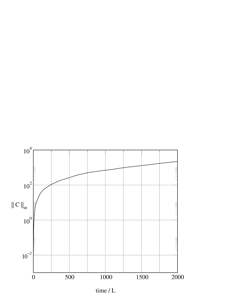
FIG. 1.: A log plot of the $\ell_{\infty}$ norm of the Hamiltonian constraint as a function of crossing time for a Stage 2 test of random Sommerfeld boundary conditions on all metric components.

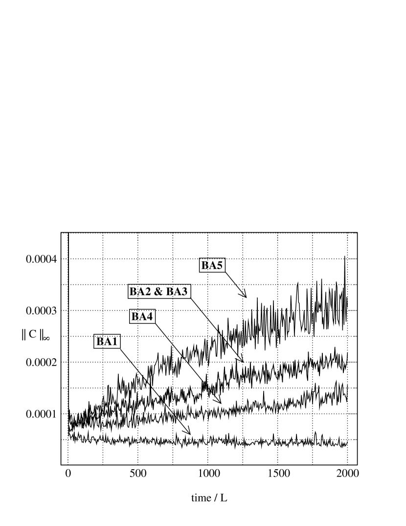
FIG. 2.: Stage two performance of the Hamiltonian constraint as a function of crossing time for the five robustly stable algorithms BA1 to BA5 .

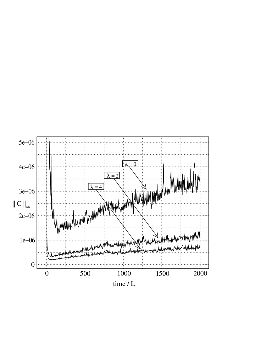
FIG. 3.: Behavior of the Hamiltonian constraint for a Stage 3 test with cubic boundary.