Gravitomagnetism and the Clock Effect

Abstract

The main theoretical aspects of gravitomagnetism are reviewed. It is shown that the gravitomagnetic precession of a gyroscope is intimately connected with the special temporal structure around a rotating mass that is revealed by the gravitomagnetic clock effect. This remarkable effect, which involves the difference in the proper periods of a standard clock in prograde and retrograde circular geodesic orbits around a rotating mass, is discussed in detail. The implications of this effect for the notion of “inertial dragging” in the general theory of relativity are presented. The theory of the clock effect is developed within the PPN framework and the possibility of measuring it via spaceborne clocks is examined.

1 Introduction

The close formal similarity between Coulomb’s law of electricity and Newton’s law of gravitation has led to a description of Newtonian gravitation in terms of a gravitoelectric field. The classical tests of general relativity can all be described via post-Newtonian gravitoelectric corrections brought about by relativity theory. Moreover, any theory that combines Newtonian gravitation and Lorentz invariance in a consistent framework must involve a gravitomagnetic field in close analogy with electrodynamics. The gravitomagnetic field is generated by the motion of matter. For instance, the mass current in the rotating Earth generates a dipolar gravitomagnetic field that has not yet been directly observed; in fact, the main objective of the GP-B is to measure this field in a polar Earth orbit via the gravitomagnetic precession of superconducting gyroscopes on board a drag-free satellite.

Gravitomagnetism had its beginning in the second half of the last century. Developments in electrodynamics led Holzmüller GHo and Tisserand FTi to postulate the existence of a solar gravitomagnetic field ande94 . In fact, attempts were made to account for the excess perihelion precession of Mercury since the planetary orbits would be affected by the gravitomagnetic field of the Sun. However, the excess perihelion precession of Mercury was successfully explained by Einstein’s general relativity theory in terms of a small relativistic correction to the Newtonian gravitoelectric potential of the Sun. It was later shown by Thirring and Lense HTh ; BM1 that general relativity also predicts a certain gravitomagnetic field for a rotating mass, but the magnitude of this field in the solar system is generally small and would lead to a retrograde precession of the planetary orbits. This Lense-Thirring precession of planetary orbits is too small to be detectable at present.

For the purposes of confronting the theory with observation, gravitomagnetic phenomena are usually described in the framework of the post-Newtonian approximation; however, it is possible to provide a fully covariant treatment of certain aspects of gravitoelectromagnetism AMa ; BJH . In fact, extensions of the Jacobi equation (i.e. the relativistic tidal equation) may be employed to identify the gravitoelectric and gravitomagnetic components of the curvature tensor in close analogy with the Lorentz force law. This analogy is incomplete, however, since the purely spatial components of the curvature tensor do not in general have an analog in the electromagnetic case; in fact, this is expected since linear gravity is a spin-2 field in contrast to the spin-1 character of the electromagnetic field.

Some of the main theoretical aspects of gravitomagnetism are discussed in Section 2. We then turn our attention to how gravitomagnetism affects the spacetime structure in general relativity. Of primary importance in this connection is the gravitomagnetic clock effect, which in its simplest form may be formulated in terms of the difference in the proper periods of two clocks moving on the same circular orbit but in opposite directions about a rotating mass. Let $\tau_{+}(\tau_{-})$ be the period for prograde (retrograde) motion, then for $r\gg 2GM/c^{2},\tau_{+}-\tau_{-}\approx 4\pi J/(Mc^{2})$. To lowest order, this remarkable result is independent of Newton’s constant of gravitation $G$ and the radius of the orbit $r$. The effect and its consequences are discussed in Section 3 for circular equatorial orbits in the Kerr geometry and the intimate connection between the clock effect and the gravitomagnetic gyroscope precession is demonstrated. The PPN approximation for this effect is developed in Section 4 and a brief discussion of its observability is given in Section 5. The sign of the clock effect is quite intriguing, as it implies that prograde equatorial clocks are slower than retrograde equatorial clocks. This is completely opposite to what would be expected on the basis of “inertial dragging”. In fact, gravitomagnetism is historically connected with the question of the origin of inertia as this was Thirring’s motivation in his original paper on gravitomagnetism HTh . The present status of the problem of inertia is the subject of Section 6. Finally, Section 7 contains a brief discussion.

Unless specified otherwise, we use units such that $G=c=1$ for the sake of convenience.

2 Gravitoelectromagnetism

This section is devoted to a brief discussion of certain essential theoretical aspects of gravitoelectromagnetism. The Larmor theorem has played an important role in the field of magnetism; therefore, we begin by an account of the gravitational analog of Larmor’s theorem.

Gravitational Larmor Theorem

A century ago, Larmor established a theorem regarding the local equivalence of magnetism and rotation 1 . That is, the basic electromagnetic force on a slowly moving particle of charge $q$ and mass $m$ can be locally replaced in the linear approximation by the inertial forces that arise if the motion is referred instead to an accelerated system in the absence of the electromagnetic field. The translational acceleration of the system is related to the electric field, ${\bf a}_{L}=-(q/m){\bf E}$, and the rotational (Larmor) frequency is related to the magnetic field via $\mbox{\boldmath$\omega$}_{L}=q{\bf B}/(2mc)$. The charge-to-mass ratio is not the same for all particles; otherwise, a geometric theory of electrodynamics could be developed along the same lines as general relativity. It turns out that in general relativity one can provide an interpretation of Einstein’s heuristic principle of equivalence via the gravitational Larmor theorem 2 . This is due to the experimentally well-established circumstance that the gravitational charge-to-mass ratio is the same for all particles. Einstein’s heuristic principle of equivalence is usually stated in terms of the gravitoelectric field, i.e. the translational acceleration of the “Einstein elevator” in Minkowski spacetime. The gravitational Larmor theorem would also involve the gravitomagnetic field, i.e. a rotation of the elevator as well.

It follows from the theoretical study of the motion of test particles as well as ideal test gyroscopes in a gravitational field that in general relativity the gravitoelectric charge is $q_{E}=-m$, while the gravitomagnetic charge is $q_{B}=-2m$; in fact, $q_{B}/q_{E}=2$ since general relativity involves the tensor potential $g_{\mu\nu}$, i.e. (linear) gravitation is a spin-2 field. Thus ${\bf a}_{L}={\bf E}$ and $\mbox{\boldmath$\omega$}_{L}=-{\bf B}/c$ in this case. Indeed ${\bf B}/c=\mbox{\boldmath$\Omega$}_{P}$ is the gravitomagnetic precession frequency of an ideal test gyroscope at rest in a gravitomagnetic field, i.e. far from a rotating source $d{\bf S}/dt=\mbox{\boldmath$\Omega$}_{P}\times{\bf S}$, where

$$\mbox{\boldmath$\Omega$}_{P}=\frac{GJ}{c^{2}r^{3}}[3(\hat{\bf r}\cdot\hat{\bf J})\hat{\bf r}-\hat{\bf J}],$$ (1)

and $J$ is the total angular momentum of the source. Let us note that a gyro spin is in effect a gravitomagnetic dipole moment that precesses in a gravitomagnetic field. Locally, the same rotation would be observed in the absence of the gravitomagnetic field but in a frame rotating with frequency $\mbox{\boldmath$\omega$}_{L}=-\mbox{\boldmath$\Omega$}_{P}$ in agreement with the gravitational Larmor theorem.

It is the goal of the GP-B to measure the gravitomagnetic gyroscope precession in a polar orbit about the Earth and thereby provide direct observational proof of the existence of the gravitomagnetic field 3 .

Gravitoelectromagnetic Field

Let us consider the gravitational field of a “nonrelativistic” rotating astronomical source in the linear approximation of general relativity. The spacetime metric may be expressed as $g_{\mu\nu}=\eta_{\mu\nu}+h_{\mu\nu}$, where $\eta_{\mu\nu}$ is the Minkowski metric. We define $\bar{h}_{\mu\nu}=h_{\mu\nu}-{1\over 2}\eta_{\mu\nu}h$, where $h={\rm tr}(h_{\mu\nu})$; then, the gravitational field equations are given by

$$\Box\bar{h}_{\mu\nu}=-16\frac{\pi G}{c^{4}}T_{\mu\nu},$$ (2)

where the Lorentz gauge condition $\bar{h}^{\mu\nu},_{\nu}=0$ has been imposed. We focus attention on the particular retarded solution of the field equations given by

$$\bar{h}_{\mu\nu}=\frac{4G}{c^{4}}\int\frac{T_{\mu\nu}(ct-|{\bf x}-{\bf x}^{\prime}|,\;{\bf x}^{\prime})}{|{\bf x}-{\bf x}^{\prime}|}\>d^{3}x^{\prime},$$ (3)

where the nature and distribution of the “nonrelativistic” source must be taken into account.

We are interested in sources such that $\bar{h}_{00}=4\Phi/c^{2}$, $\bar{h}_{0i}=-2A_{i}/c^{2}$ and $\bar{h}_{ij}=O(c^{-4})$, where $\Phi(t,{\bf x})$ is the gravitoelectric potential, ${\bf A}(t,{\bf x})$ is the gravitomagnetic vector potential and we neglect all terms of order $c^{-4}$ and lower including the tensor potential $\bar{h}_{ij}(t,{\bf x})$. It follows that $T^{00}/c^{2}=\rho$ is the effective gravitational charge density and $T^{0i}/c=j^{i}$ is the corresponding current. Thus, far from the source

$$\Phi\sim\frac{GM}{r},\;\;\;\;\;\;\;\;\;\;\;{\bf A}\sim\frac{G}{c}\frac{{\bf J}\times{\bf r}}{r^{3}},$$ (4)

where $M$ and ${\bf J}$ are the total mass and angular momentum of the source, respectively. It follows from the Lorentz gauge condition that

$$\frac{1}{c}\frac{\partial\Phi}{\partial t}+\mbox{\boldmath$\nabla$}\cdot\left({1\over 2}{\bf A}\right)=0,$$ (5)

since the other three equations $(\bar{h}^{i\mu},_{\mu}=0)$ all involve terms that are of $O(c^{-4})$ and therefore neglected. The spacetime metric involving the gravitoelectromagnetic (“GEM”) potentials is then given by

$$-ds^{2}=-c^{2}\left(1-{2\over c^{2}}\Phi\right)dt^{2}-{4\over c}({\bf A}\cdot d{\bf x})dt+\left(1+{2\over c^{2}}\Phi\right)\delta_{ij}dx^{i}dx^{j}.$$ (6)

The GEM fields are defined by

$${\bf E}=-\mbox{\boldmath$\nabla$}\Phi-{1\over c}{\partial\over\partial t}\left({1\over 2}{\bf A}\right),\;\;\;\;\;\;\;\;{\bf B}=\mbox{\boldmath$\nabla$}\times{\bf A},$$ (7)

in close analogy with electrodynamics. It follows from the field equations (2) and the gauge condition (5) that

$$\mbox{\boldmath$\nabla$}\cdot{\bf E}=4\pi G\rho,$$ (8)

$$\mbox{\boldmath$\nabla$}\cdot\left({1\over 2}{\bf B}\right)=0,$$ (9)

$$\mbox{\boldmath$\nabla$}\times{\bf E}=-{1\over c}{\partial\over\partial t}\left({1\over 2}{\bf B}\right),$$ (10)

$$\mbox{\boldmath$\nabla$}\times\left({1\over 2}{\bf B}\right)={1\over c}{\partial\over\partial t}{\bf E}+{4\pi\over c}G\>{\bf j}\>,$$ (11)

which are the Maxwell equations for the GEM field. Using classical electrodynamics as a guide, one can investigate the various implications of these equations 4 . A thorough approach to the determination of the gravitomagnetic field of a rotating mass (such as the Earth) is contained in the papers of Teyssandier 5 .

The fact that the magnetic parts of equations (8) - (11) always appear with a factor of $1/2$ as compared to standard electrodynamics is due to the circumstance that the effective gravitomagnetic charge is twice the gravitoelectric charge. That is, $Q_{E}=M$ and $Q_{B}=2M$ are the effective gravitoelectric and gravitomagnetic charges of the source.

The linear approximation of general relativity involves a spin-2 field. This field, once its spatial components are neglected, can be interpreted in terms of a gravitoelectromagnetic vector potential. To sustain the electromagnetic analogy, however, we need to require that the gravitomagnetic charge be twice the gravitoelectric charge. This factor of 2 is a remnant of the spin-2 character of the original field, while for a pure spin-1 field (i.e. the electromagnetic field) the ratio of the magnetic charge to the electric charge is unity.

The equation of motion of a test particle of mass $m$ in this linear gravitational field can be obtained from the variational principle $\delta\int{\cal L}dt=0$, where ${\cal L}=-mcds/dt$ is given by

$${\cal L}=-mc^{2}\left[1-{v^{2}\over c^{2}}-{2\over c^{2}}\left(1+{v^{2}\over c^{2}}\right)\Phi+{4\over c^{3}}{\bf v}\cdot{\bf A}\right]^{1/2},$$ (12)

using equation (6). To linear order in $\Phi$ and ${\bf A}$, one can write (12) as

$${\cal L}=-mc^{2}\left(1-{v^{2}\over c^{2}}\right)^{1/2}+m\gamma\left(1+{v^{2}\over c^{2}}\right)\Phi-{2m\over c}\gamma{\bf v}\cdot{\bf A}.$$ (13)

Let us note that the deviation of equation (13) from a free-particle Lagrangian is given to lowest order in ${\bf v}/c$ by $m\Phi-2m{\bf A}\cdot{\bf v}/c$. This deviation would be of the form $j_{\mu}A^{\mu}$ in electrodynamics; therefore, the slow motion of the test particle is very similar to that of a charged particle in electrodynamics except that here $q_{E}=-m$ and $q_{B}=-2m$ as expected. It thus follows from the geodesic motion of a test particle of mass $m$ far from the source in this gravitational background that the canonical momentum of the particle is given approximately by ${\bf p}+(-2m/c){\bf A}$, where ${\bf p}$ is the kinetic momentum. In this electrodynamic analogy, the attractive nature of gravity is reflected in our convention of positive gravitational charges for the source and negative gravitational charges for the test particle. The gravitomagnetic charge is always twice the gravitoelectric charge as a consequence of the tensorial character of the gravitational potentials in general relativity.

The gauge transformations

$$\Phi\rightarrow\Phi-{1\over c}{\partial\psi\over\partial t},\;\;\;\;\;{\bf A}\rightarrow{\bf A}+2\mbox{\boldmath$\nabla$}\psi,$$ (14)

leave the GEM fields (7) and hence the GEM equations (8)-(11) invariant. The Lorentz gauge condition (5) is also satisfied provided $\Box\psi=0$. However, the quantity $-q_{E}\Phi+q_{B}{\bf A}\cdot{\bf v}/c$ in the Lagrangian is not invariant under the gauge transformation (14). The gauge invariance of this Lagrangian is restored, however, if the gauge function $\psi$ is independent of time, $\partial\psi/\partial t=0$. In this case, we can start from a coordinate transformation $t\rightarrow t-4\psi({\bf x})/c^{3}$ in the metric (6) resulting in the gauge transformations (14) with $\Phi$ left invariant.

The gravitational field corresponding to the metric (6) is given by the Riemann curvature tensor

$$R_{\mu\nu\rho\sigma}={1\over 2}(h_{\mu\sigma,\;\nu\rho}+h_{\nu\rho,\;\mu\sigma}-h_{\nu\sigma,\;\mu\rho}-h_{\mu\rho,\nu\sigma}),$$ (15)

where $h_{00}=2\Phi/c^{2}$ and $h_{ij}=(2\Phi/c^{2})\delta_{ij}$ are gravitoelectric and of $O(c^{-2})$, while $h_{0i}=-2A_{i}/c^{2}$ is gravitomagnetic and of $O(c^{-3})$. The components of the curvature tensor as measured by the standard geodesic observers are given by $R_{\mu\nu\rho\sigma}\lambda^{\mu}_{(\alpha)}\lambda^{\nu}_{(\beta)}\lambda^{\rho}_{(\gamma)}\lambda^{\sigma}_{(\delta)}$, where $\lambda^{\mu}_{(\alpha)}$ is the tetrad frame of the test observer. In the linear approximation under consideration here, $\lambda^{\mu}_{(\alpha)}$ is in effect equal to $\delta^{\mu}_{\alpha}$ in the calculation of the measured curvature. The components of this tensor may be expressed in the form of a symmetric $6\times 6$ matrix ${\cal R}=({\cal R}_{AB})$, where $A$ and $B$ range over (01, 02, 03, 23, 31, 12); hence,

$${\cal R}=\begin{pmatrix}{\cal E}&{\cal B}\\ {\cal B}^{T}&{\cal S}\end{pmatrix}\,,$$ (16)

where ${\cal E}$ and ${\cal S}$ are symmetric $3\times 3$ matrices and ${\cal B}$ is traceless. We find that the electric and magnetic components of the curvature are given by

$${\cal E}_{ij}={1\over c^{2}}E_{j,i}+O(c^{-4}),$$ (17)

$${\cal B}_{ij}=-{1\over c^{2}}B_{j,i}+{1\over c^{3}}\epsilon_{ijk}{\partial E_{k}\over\partial t}+O(c^{-4}),$$ (18)

and the spatial components are given by

$${\cal S}_{ij}=-{1\over c^{2}}E_{j,i}+{1\over c^{2}}(\mbox{\boldmath$\nabla$}\cdot{\bf E})\delta_{ij}+O(c^{-4}).$$ (19)

That ${\cal B}$ is traceless is consistent with equation (9) and the fact that ${\cal E}$ and ${\cal S}$ are symmetric is consistent with equation (10) at $O(c^{-4})$. It is therefore clear that gravitoelectromagnetism permeates every aspect of general relativity: the gravitational potentials (GEM potentials), the connection (GEM field) and the curvature. In the exterior of the rotating source, the spacetime is Ricci-flat and hence ${\cal S}=-{\cal E}$, ${\cal E}$ is traceless and ${\cal B}$ is symmetric. These restrictions on the curvature are consistent with the GEM field equations (8)-(11) in the source-free region.

The general treatment of gravitoelectromagnetism presented here has been based on a certain approximate form of the linear gravitation theory and can be used in the theoretical description of many interesting gravitational phenomena. In particular, we use this formalism below to investigate the microphysical implications of the gravitomagnetic precession of spin.

Free Fall is not Universal

The assumption that all free test particles fall in the same way in a gravitational field is reflected in general relativity via the geodesic hypothesis. That is, the worldline of a free test particle is an intrinsic property of the spacetime manifold and is independent of the intrinsic aspects of the particle. In this way, general relativity is a geometric theory of gravitation. This circumstance originates from the well-tested equality of inertial and gravitational masses.

An important consequence of Einstein’s geometric theory of gravitation is the fact that an ideal test gyroscope would precess in the gravitomagnetic field of a rotating source. Here we pose the question of whether all spins should “precess” like a gyroscope; evidently, the treatment of intrinsic spin would go beyond classical general relativity. It follows from the consideration of spin-rotation-gravity coupling that the intrinsic spin of a particle (e.g. a nucleus) would couple to the gravitomagnetic field of a rotating source (such as the Earth) via the interaction Hamiltonian

$${\cal H}=\mbox{\boldmath$\sigma$}\cdot\mbox{\boldmath$\Omega$}_{P}$$ (20)

such that the Heisenberg equations of motion for the spin would be formally the same as that of an ideal test gyro 6 . Intuitively, this interaction is due to the coupling of the gravitomagnetic dipole moment of the particle with the gravitomagnetic field just as would be expected from the electromagnetic analogy. It follows from equation (20) that the particle is subject to a gravitational Stern-Gerlach force given by

$${\bf F}=-\mbox{\boldmath$\nabla$}(\mbox{\boldmath$\sigma$}\cdot\mbox{\boldmath$\Omega$}_{P})$$ (21)

that is purely dependent upon its spin and not its mass and therefore violates the universality of free fall.

The point is that a particle is in general endowed with mass and spin in addition to other intrinsic properties; indeed, the irreducible unitary representations of the inhomogeneous Lorentz group are characterized by mass and spin. In its interaction with a gravitational field, the mass interacts primarily with the gravitoelectric field while the spin interacts primarily with the gravitomagnetic field. Whereas the former dominant interaction is consistent with the universality of free fall, the latter is not. For instance, the bending of light by the gravitational field of a rotating source depends on the state of polarization of the radiation. The differential deflection of polarized radiation by the Sun is too small to be measurable at present. The predicted violation is also extremely small for a nucleus in a laboratory on the Earth: the weight of the particle is $w=mg_{\oplus}(1\pm\epsilon)$, depending on whether the spin is polarized vertically up or down and $\epsilon\sim 10^{-29}$. Thus the predicted violation of the universality of free fall is extremely small.

It may still be possible to measure this relativistic quantum gravitational effect by detecting the change in the energy of a particle in the laboratory when its spin is flipped. This would require, for instance, significant refinements in modern variations of NMR and optical pumping techniques, since

$$\hbar\Omega_{P}\sim\frac{\hbar GJ}{c^{2}R^{3}}={cJ\over R}\left(\frac{L_{P}}{R}\right)^{2}\sim 10^{-28}{\rm eV}$$ (22)

is a factor of $10^{4}$ below the sensitivity of recent experiments 7 . Here $L_{P}$ is the Planck length, $L_{P}^{2}=\hbar G/c^{3}$, $J$ is the angular momentum of the Earth and $R$ is its average radius. The smallest detected energy shift is about $10^{-24}$eV corresponding to a frequency shift of 2 nHz 7 . However, it appears that significantly lower energy shifts may soon be detectable 8 .

To clarify the nature of the force (21), let us consider the motion of a classical spinning test body in a stationary gravitational field. Such a system is necessarily extended and thus couples to spacetime curvature resulting in a Mathisson-Papapetrou force

$$F_{\alpha}={c\over 2}R_{\alpha\beta\mu\nu}u^{\beta}S^{\mu\nu}=cR_{\alpha\mu\beta\nu}u^{\beta}S^{\mu\nu},$$ (23)

where $S^{\mu\nu}$ is the spin tensor of the system, $u^{\mu}$ is the velocity vector such that $S^{\mu\nu}u_{\nu}=0$ and the spin vector is given by

$$S_{\mu}={1\over 2}(-g)^{1/2}\epsilon_{\mu\nu\rho\sigma}u^{\nu}S^{\rho\sigma}.$$ (24)

For the calculation of $F_{\alpha}$, it suffices to set, in the linear approximation, $u^{\alpha}\approx(1,\>0,\>0,\>0)$, $S^{0i}\approx 0$ and $S^{ij}\approx-\epsilon^{ijk}S_{k}$. Then, $F_{0}\approx 0$ and

$$F_{i}\approx c{\cal B}_{ij}S^{j}=-{1\over c}B_{j,i}S^{j}=-(\mbox{\boldmath$\Omega$}_{P})_{j,i}S^{j},$$ (25)

in agreement with equation (21). Thus the existence of the force (21) may be ascribed to the intrinsic nonlocality of a particle in the quantum theory and hence the coupling of spin to the magnetic part of the spacetime curvature in a stationary field.

It is important to remark here that our considerations are distinct from proposals to measure the classical spin-spin force as discussed in 4 . Our results ultimately follow from detailed considerations of Dirac-type wave equations in the gravitational field of a rotating mass (see the references cited in 6 ); however, one can arrive at equations (20)-(21) on the basis of certain general arguments such as the local isotropy of space, the extended hypothesis of locality and the gravitational Larmor theorem 6 .

Assuming the approximate validity of equations (20)-(21), it would be difficult to imagine a basic gravitational theory founded purely on the universality of free fall and Riemannian geometry. However, such a theoretical structure would clearly be an excellent effective theory in the macrophysical domain.

GEM Stress-Energy Tensor

Let us imagine a congruence of geodesic test particles in a gravitational field. Taking one of the test particles as the reference observer, how does the motion of the other neighboring test particles appear to the fiducial observer? The result is best expressed in a Fermi coordinate system that is set up along the reference worldline. Let $X^{\mu}=(\tau,{\bf X})$ be the Fermi coordinates of the test particles, while the reference observer is at the origin of spatial Fermi coordinates. Then the equation of motion of the test particles is given by the generalized Jacobi equation

$$\frac{d^{2}X^{i}}{d\tau^{2}} + {}^{F}\!R_{0i0j}X^{j}+2\>^{F}\!R_{ikj0}V^{k}X^{j}+(2\>^{F}\!R_{0kj0}V^{i}V^{k}$$ (26)

$$+ {2\over 3}\>^{F}\!R_{ikjl}V^{k}V^{l}+{2\over 3}\>^{F}\!R_{0kjl}V^{i}V^{k}V^{l})X^{j}=0,$$ (27)

which is valid to first order in the relative separation ${\bf X}$ and to all orders in the relative velocity ${\bf V}=d{\bf X}/d\tau$. Here ${}^{F}\!R_{\alpha\beta\gamma\delta}(\tau)$ are components of the curvature tensor as measured by the fiducial observer, i.e. they are the projections of the Riemann tensor onto the nonrotating tetrad frame of the reference observer. Neglecting the second and third order terms in the relative rate of separation, equation (27) can be written as the GEM analog of the Lorentz force law

$$m\frac{d^{2}{\bf X}}{d\tau^{2}}=q_{E}{\bf E}+q_{B}{\bf V}\times{\bf B},$$ (28)

where $q_{E}=-m$, $q_{B}=-2m$ and

$$E_{i}=\>^{F}\!R_{0i0j}(\tau)X^{j},\;\;B_{i}=-{1\over 2}\epsilon_{ijk}\;^{F}\!R_{jk0l}(\tau)X^{l}.$$ (29)

It is important to notice that the spacetime interval in the neighborhood of the reference worldline can be expressed in Fermi coordinates as $-ds^{2}=\>^{F}\!g_{\mu\nu}\>dX^{\mu}dX^{\nu}$, where

$${}^{F}\!g_{00}=-1-\>^{F}\!R_{0i0j}(\tau)X^{i}X^{j}+\cdots,$$ (30)

$${}^{F}\!g_{0i}=-{2\over 3}\>^{F}\!R_{0jik}(\tau)X^{j}X^{k}+\cdots,$$ (31)

$${}^{F}\!g_{ij}=\delta_{ij}-{1\over 3}\>^{F}\!R_{ikjl}(\tau)X^{k}X^{l}+\cdots.$$ (32)

Letting ${}^{F}\!g_{00}=-1+2\Phi$ and ${}^{F}\!g_{0i}=-2A_{i}$, we find that

$$\Phi=-{1\over 2}\>^{F}\!R_{0i0j}X^{i}X^{j},\;\;\;A_{i}={1\over 3}\>^{F}\!R_{0jik}X^{j}X^{k},$$ (33)

so that the corresponding GEM fields using equation (7) agree with the results in equation (29) to linear order in the separation ${\bf X}$. One can verify directly that $\mbox{\boldmath$\nabla$}\cdot{\bf B}=0$ and $\mbox{\boldmath$\nabla$}\times{\bf E}=0$, so that the source-free pair of Maxwell’s equations are satisfied along the reference worldline. Moreover, it is possible to combine the GEM fields together to form a GEM Faraday tensor $F_{\alpha\beta}$,

$$F_{\alpha\beta}=-\>^{F}\!R_{\alpha\beta 0l}X^{l},$$ (34)

such that $F_{0i}=-E_{i}$ and $F_{ij}=\epsilon_{ijk}B_{k}$ as in standard electrodynamics. Then the other pair of Maxwell’s equations is given by $F^{\alpha\beta},_{\beta}=4\pi J^{\alpha}$, where $J^{\alpha}(\tau,{\bf X})$ is easily obtained to linear order in ${\bf X}$ using equation (34). $J^{\alpha}$ is a conserved current such that $J_{\alpha}(\tau,{\bf 0})=-\>^{F}\!R_{\alpha 0}/4\pi$ along the fiducial trajectory. This treatment should be compared and contrasted with the linear approximation developed above, in particular, the GEM current is different here.

It is now possible to develop the classical field theory of the GEM field in the Fermi frame; in particular, one can define the Maxwell stress-energy tensor and the corresponding angular momentum for the GEM field. Thus

$${\cal T}^{\alpha\beta}(\tau,{\bf X})={1\over 4\pi}\left(F^{\alpha}\!{}_{\gamma}F^{\beta\gamma}-{1\over 4}\eta^{\alpha\beta}F_{\gamma\delta}F^{\gamma\delta}\right)$$ (35)

is the Maxwell stress-energy tensor for the GEM field that is quadratic in the spatial separation and vanishes at the location of the fiducial observer. Physical measurements do not occur at a point, as already emphasized by Bohr and Rosenfeld 9 ; moreover, the fiducial observer is arbitrary here. Therefore, a physically more meaningful quantity is obtained by averaging equation (35) over a sphere of radius $\epsilon L$ in the Fermi system. Here $L$ is a constant invariant lengthscale associated with the gravitational field. We find that

$$<{\cal T}_{\alpha\beta}(\tau,{\bf X})>=\epsilon^{2}C_{0}L^{2}\tilde{T}_{\mu\nu\rho\sigma}\lambda^{\mu}_{(\alpha)}\lambda^{\nu}_{(\beta)}\lambda^{\rho}_{(0)}\lambda^{\sigma}_{(0)},$$ (36)

where $C_{0}$ is a constant numerical factor and

$$\tilde{T}_{\mu\nu\rho\sigma}={1\over 2}\left(R_{\mu\xi\rho\zeta}R_{\nu\;\sigma}^{\;\>\xi\;\zeta}+R_{\mu\xi\sigma\zeta}R_{\nu\;\rho}^{\;\>\xi\;\zeta}\right)-{1\over 4}g_{\mu\nu}R_{\alpha\beta\rho\gamma}R^{\alpha\beta\;\gamma}_{\;\;\;\>\sigma}.$$ (37)

For a Ricci-flat spacetime, $\tilde{T}_{\mu\nu\rho\sigma}$ reduces to the Bel-Robinson tensor $T_{\mu\nu\rho\sigma}$; in this case, $R_{\alpha\beta\gamma\delta}$ reduces to the Weyl tensor $C_{\alpha\beta\gamma\delta}$ and in equation (37) $C_{\alpha\beta\rho\gamma}C^{\alpha\beta\;\gamma}_{\;\;\;\>\sigma}=(K/4)g_{\rho\sigma}$ with $K=C_{\alpha\beta\gamma\delta}C^{\alpha\beta\gamma\delta}$.

The magnitude of $C_{0}$ depends on whether we average over the surface or the volume of the sphere; in any case, one can always absorb $C_{0}$ into the definition of $L$. Thus the pseudo-local GEM stress-energy tensor may be defined for any observer with the tetrad frame $\lambda^{\mu}_{(\alpha)}$ as

$$T_{(\alpha)(\beta)}=L^{2}\tilde{T}_{\mu\nu\rho\sigma}\lambda^{\mu}_{(\alpha)}\lambda^{\nu}_{(\beta)}\lambda^{\rho}_{(0)}\lambda^{\sigma}_{(0)}.$$ (38)

In this way, the pseudo-local GEM energy density, Poynting flux and stresses are defined up to a common multiplicative factor.

It is important to note that the spatial components of the curvature have been ignored in our construction of the GEM tensor $T_{(\alpha)(\beta)}$. For a Ricci-flat spacetime, however, the spatial components of the curvature are simply related to its electric components; therefore, the pseudo-local tensor defined via equation (38) using the Bel-Robinson tensor contains the full (Weyl) curvature tensor and is thus the gravitational stress-energy tensor.

It follows from a simple application of these results to the field of a rotating mass that there exists a steady Poynting flux of gravitational energy in the exterior field of a rotating mass.

Oscillations of a Charged Rotating Black Hole

Imagine a black hole of mass $M$, charge $Q$ and angular momentum $J$ that is perturbed by external radiation. The black hole is stationary and axisymmetric; therefore, the perturbation is expressible in terms of eigenmodes ${\cal P}(r,\theta)\,{\rm exp}(-i\omega t$
$+im_{j}\phi)$, where ${\cal P}$ depends upon the frequency of the radiation, the total angular momentum parameters of the eigenmode $(j,m_{j})$ and the spin of the external field. It turns out that for a Fourier sum of such eigenmodes, the response of the black hole far away and at late times is dominated by a superposition of certain damped oscillations of the form $A\,{\rm exp}(-i\omega t)$, where $\omega=\omega_{BH}-i\Gamma_{BH}$ with $\Gamma_{BH}\geq 0$. For these quasinormal modes, the amplitude $A$ depends, among other things, on the strength of the perturbation while $\omega$ depends only on the black hole parameters $(M,Q,J)$. Moreover, these black hole oscillations are in general denumerably infinite and are numbered as $n=0,1,2,\cdots$, such that $n=0$ is least damped and $\Gamma_{BH}$ increases with $n$. The intrinsic ringing of a black hole is due to the fact that once perturbed, the black hole undergoes characteristic damped oscillations in order to return to a stationary state.

The fundamental modes of oscillations of black holes were originally found by numerical experiments and initial attempts to explain the numerical results via the properties of black hole effective potentials were unsuccessful 10 . The solution of the problem was first given around 1980 11 . This work provided the stimulus for many subsequent investigations by a number of authors 12 . A detailed discussion of black hole oscillations is contained in 13 .

For the modes of oscillation of a charged rotating black hole, the only reliable results are for $j\geq|m_{j}|\gg 1$. Expressions for $(\omega_{BH},\Gamma_{BH})$ have been obtained in the case of $j=|m_{j}|\gg 1$ for a general Kerr-Newman black hole; however, the results have been generalized to the case of $j>|m_{j}|\gg 1$ only for a slowly rotating charged black hole 14 . To express $(\omega_{BH},\Gamma_{BH})$ in terms of $(M,J,Q)$ in the latter case, let $\omega_{\rm K}(r)=(Mr^{-3}-Q^{2}r^{-4})^{1/2}$ be the “Keplerian” frequency for the motion of a neutral particle in a circular geodesic orbit of radius $r$ about a Reissner-Nordström black hole of mass $M$ and charge $Q$. Here we use Boyer-Lindquist type of coordinates for the Kerr-Newman geometry. Timelike circular geodesic orbits exist down to a null orbit of radius $r_{N}$ such that $2r_{N}=3M+(9M^{2}-8Q^{2})^{1/2}$. Let $\omega_{N}=\omega_{\rm K}(r_{N})$, then it can be shown that for a slowly rotating black hole

$$\omega_{BH}\approx\pm j\omega_{N}+m_{j}\Omega_{N},$$ (39)

where

$$\Omega_{N}=\frac{J}{r_{N}^{3}}\left(1-\frac{Q^{2}}{Mr_{N}}\right)\frac{r_{N}+M}{r_{N}-M},$$ (40)

is an effective black hole rotation frequency. The $(2j+1)$-fold degeneracy in the spectrum of oscillations of the spherical black hole is removed by its rotation. We note that $\Omega_{N}$ is proportional to the gravitomagnetic precession frequency at $r_{N}$. Moreover,

$$\Gamma_{BH}\approx\left(n+{1\over 2}\right)\left(2-3{M\over r_{N}}\right)^{1/2}\left(\omega_{N}\mp{m_{j}\over j}Q_{*}\Omega_{N}\right),$$ (41)

where $n=0,1,2,\cdots$ is the mode number and $Q_{*}=6MQ^{2}/[r_{N}(9M^{2}-8Q^{2})]$. It is interesting to note that if the black hole is charged, the rotation removes the degeneracy of the damping factor as well. Moreover, in the formulas (39) and (41) if $(\omega_{BH},\Gamma_{BH})$ is a ringing mode, then so is $(-\omega_{BH},\Gamma_{BH})$. These results are independent of the spin of the perturbing field, since they are valid for states of high total angular momentum $j\geq|m_{j}|\gg 1$.

3 Structure of Time and Relativistic Precession

Let us now return to the gravitomagnetic temporal structure around a rotating source. The gravitomagnetic clock effect involves a coupling between the orbital motion of clocks and the rotation of the source. On the other hand, the gravitomagnetic gyroscope precession occurs even for a gyroscope at rest in the exterior field of a rotating source. Nevertheless, there is a general physical connection between relativistic precession and temporal structure. This is not surprising since the operational definition of time ultimately involves counting a definite period and simple precession is uniform periodic motion. It is the purpose of this section to explain this relationship. We do this in several steps in the context of Kerr geometry with

$$-ds^{2}=-dt^{2}+\frac{\Sigma}{\Delta}\hskip 3.61371ptdr^{2}+\Sigma\hskip 3.61371ptd\theta^{2}+(r^{2}+a^{2})\sin^{2}\theta\hskip 3.61371ptd\phi^{2}\hskip 56.9055pt$$ (42)

$$\hskip 199.16928pt+\frac{R_{g}r}{\Sigma}(c\hskip 3.61371ptdt-a\sin^{2}\theta\hskip 3.61371ptd\phi)^{2},$$ (43)

where $\Sigma=r^{2}+a^{2}\cos^{2}\theta$ and $\Delta=r^{2}-R_{g}r+a^{2}$. Here $R_{g}=2GM/c^{2}$ is the gravitational radius of the source and the Kerr parameter $a=J/Mc$ is a lengthscale characteristic of the rotation of the source. For $M=0$ and $a\neq 0$, the spacetime given by (43) is flat as expected. For $a=0$ and $M\neq 0$, the metric (43) represents the Schwarzschild geometry. Finally, for $a=0$ and $M=0$ we have the metric of an inertial frame expressed in spherical coordinates $(r,\theta,\phi)$.

Let us first imagine an accelerated observer in an inertial frame. Suppose that this observer carries along its worldline an ideal pointlike test gyroscope so that there is no net torque on the gyroscope and its spin axis is therefore nonrotating. To simplify matters, let us first assume that the path is a circle of radius $r$ in the $(x,y)$-plane with its center at the origin of coordinates. According to the standard static observers in the inertial frame, the accelerated observer moves with uniform frequency $\omega_{*}\hat{{\bf z}}$. The transformation between the inertial frame and the rest frame of the rotating observer involves a simple rotation of frequency $\omega_{*}$; therefore, from the viewpoint of the standard (i.e. static) observers in the rotating frame a natural operational way to keep the direction of the gyroscope spin axis nonrotating is to imagine fixing this axis at some initial time with respect to the axes of the rotating frame, but then continuously rotating it backward with frequency $\omega_{*}$. In this way, the spin direction would remain fixed in the inertial frame if the rotation of the observer were virtual. In reality, however, the observer’s proper time $\tau$ is related to $t$ by $d\tau=dt\hskip 3.61371pt(1-v^{2}/c^{2})^{1/2}$, where $v=r\omega_{*}$; hence, the backward rotation of the spin occurs with respect to the rotating observer’s proper time, i.e. with frequency $\omega_{*}(dt/d\tau)$. From the standpoint of the standard inertial observers, the time dilation causes the spin direction to overcompensate and hence the spin direction is not fixed but precesses with the Thomas precession frequency ${\bf\omega}_{{\rm T}}=-{\bf\omega}_{*}(dt/d\tau)+{\bf\omega}_{*}$. This amounts to a precession of frequency $\omega_{*}(\gamma-1)$ in a sense that is opposite to that of the rotation of the comoving observer; moreover, the generalization to arbitrary acceleration can be simply carried out by means of the Frenet procedure. That is, a Frenet frame can be set up along the path of the observer in space; then, $\omega_{*}=v/R(t)$, where $R(t)$ is the radius of the curvature at each instant of time $t$.

The intimate connection between time dilation and Thomas precession in Minkowski spacetime can be extended to a gravitational field. Therefore, let us imagine next that the motion described above is the geodesic motion of a free test particle carrying an ideal test gyroscope around a spherical mass $M$. Let $\omega_{{\rm K}}=d\phi/dt$ be the Keplerian frequency as perceived by static inertial observers at infinity; then, $\omega^{2}_{{\rm K}}=GM/r^{3}$, where $r$ is the Schwarzschild radius of the circular orbit. The proper frequency in this case is $\omega=\Gamma\omega_{{\rm K}}$, where $\Gamma=dt/d\tau=(1-3GM/c^{2}r)^{-1/2}$. The gravitational time dilation involves the static “gravitational redshift” effect of $-g_{00}=1-2GM/c^{2}r$ in the Schwarzschild geometry as well as the azimuthal motion $r^{2}(d\phi/dt)^{2}=GM/r$ resulting in the factor of 3 in $\Gamma$. This situation is reminiscent of the spin-orbit coupling in the motion of the electron around the nucleus in the hydrogen atom; however, there are subtle differences between the electromagnetic and gravitational cases. In this case, the spin precession frequency is given by the Fokker frequency $\omega_{{\rm F}}=\omega-\omega_{{\rm K}}$, and the sense of precession is in the same sense as the orbital motion. This gravitational analog of the Thomas precession has a simple and transparent explanation in terms of Einstein’s principle of equivalence. According to this heuristic principle, an observer ${\cal O}$ in a gravitational field is locally equivalent to an observer ${\cal O}^{\prime}$ in Minkowski spacetime with an acceleration that is equal in magnitude but opposite in direction to the Newtonian gravitational “acceleration” of ${\cal O}$. The gravitational (Fokker) precession is thus locally equivalent to Thomas precession with the direction of acceleration reversed. It follows that the Fokker precession is in the same sense as the orbital motion. For an arbitrary accelerated observer in a gravitational field with velocity $u^{\mu}=dx^{\mu}/d\tau$ and acceleration $a^{\mu}=Du^{\mu}/d\tau$, the nonrotating equation of motion for the torque-free pointlike spin vector $(u_{\mu}S^{\mu}=0)$ is

$$\frac{dS^{\mu}}{d\tau}+\Gamma^{\mu}_{\alpha\beta}\hskip 3.61371ptu^{\alpha}S^{\beta}=u^{\mu}a_{\nu}S^{\nu},$$ (44)

so that both Fokker and Thomas precessions would be present for accelerated motion in Schwarzschild geometry.

The gravitomagnetic precession of a gyroscope is in a similar way related to the temporal structure brought about by the rotation of the source. However, the situation here is more complicated than the gravitoelectric Fokker precession since the temporal structure is affected by the coupling of orbital motion with the angular momentum of the source.

Specifically, let us imagine stable circular geodesic orbits in the equatorial plane of the Kerr source (43). It can be shown that

$$\frac{dt}{d\phi}=\frac{a}{c}\pm\frac{1}{2\pi}T_{{\rm K}}\hskip 14.45377pt,\hskip 14.45377pt\frac{d\tau}{d\phi}=\pm\frac{1}{2\pi}T_{{\rm K}}\hskip 3.61371pt(1\pm 2\alpha-3R_{g}/2r)^{1/2}\,,$$ (45)

where $T_{{\rm K}}=2\pi/\omega_{{\rm K}}$ is the Keplerian period of the orbit and $\alpha=a\hskip 3.61371pt\omega_{{\rm K}}/c$. Here the upper (lower) sign refers to a prograde (retrograde) orbit. It follows that the orbital period is given by

$$t_{\pm}=T_{{\rm K}}\hskip 3.61371pt(1\pm\alpha)\hskip 14.45377pt,\hskip 14.45377pt\tau_{\pm}=T_{{\rm K}}\hskip 3.61371pt(1\pm 2\alpha-3R_{g}/2r)^{1/2}\,.$$ (46)

Let us first note that $t_{+}-t_{-}=4\pi a/c$ and $\tau^{2}_{+}-\tau^{2}_{-}=4\alpha T^{2}_{{\rm K}}$. Since $\tau_{+}+\tau_{-}=2T_{{\rm K}}+O(c^{-2})$, we find that $\tau_{+}-\tau_{-}\approx 4\pi a/c$. In fact, $\tau_{+}-\tau_{-}$ monotonically decreases as a function of $r$ and approaches $4\pi a/c$ as $r\rightarrow\infty$. Thus a prograde clock moves more slowly than a retrograde clock according to comoving observers as well as the standard asymptotically inertial observers at infinity; moreover, $\tau_{+}-\tau_{-}\approx 4\pi a/c$ for $r\gg R_{g}$. This remarkable gravitomagnetic clock effect has been discussed in some detail in recent publications JMC -WBB . This classical effect is in some sense the gravitomagnetic analog of the topological Aharonov-Bohm effect; in fact, let us note that far from a finite rotating source $\tau_{+}-\tau_{-}$ is nearly a constant independent of the “distance” $r$ and the gravitational coupling constant $G$. These aspects of the clock effect have been discussed in detail elsewhere BFD .

Let us now imagine two clocks moving in opposite directions on a stable circular geodesic orbit of radius $r$ in the equatorial plane of the Kerr source. Suppose that at $t_{0}=0$, they are both at $\phi_{0}=0$; let us denote the event at which the clocks next meet again by $(t_{1},\phi_{1})$. It follows from equation (45) that $2\pi t_{1}=\phi_{1}T_{{\rm K}}(1+\alpha)$ for the prograde clock and $2\pi t_{1}=(2\pi-\phi_{1})T_{{\rm K}}(1-\alpha)$ for the retrograde clock. Thus $\phi_{1}=\pi(1-\alpha)$ and $t_{1}=T_{{\rm K}}(1-\alpha^{2})/2$. Moreover, $\tau_{+}^{2}(\phi_{1})-\tau^{2}_{-}(\phi_{1})=\alpha T^{2}_{{\rm K}}(\alpha^{2}+3R_{g}/2r)$, which is negligibly small for clocks in orbit about astronomical sources in the solar system; in fact, $\tau_{+}(\phi_{1})-\tau_{-}(\phi_{1})\sim O(c^{-4})$. The next time the clocks meet is at $(t_{2},\phi_{2})$, which bears the same relationship to $(t_{1},\phi_{1})$ as $(t_{1},\phi_{1})$ to $(t_{0},\phi_{0})$; therefore, $\phi_{2}=2\pi(1-\alpha)$ and $t_{2}=T_{{\rm K}}(1-\alpha^{2})$. In general, the nth time the clocks meet is at $(t_{n},\phi_{n})$ with $\phi_{n}=n\pi(1-\alpha)$ modulo $2\pi$ and $t_{n}=nT_{{\rm K}}(1-\alpha^{2})/2$.

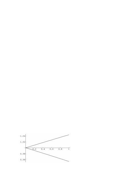
Consider now the behavior of the diametrical line joining these events to the origin of the spatial coordinates. For $a=0$, i.e. in the Schwarzschild case, this line is fixed as the clocks repeatedly meet at two diametrically opposite points. However, for $a\neq 0$ the line precesses in the opposite sense as the rotation of the source with the precession frequency given approximately by (cf. Fig. 1)

$$\frac{\pi-\phi_{1}}{\tau_{+}(\phi_{1})}=\frac{GJ}{c^{2}r^{3}}+O(c^{-4}),$$ (47)

which at this order is in agreement with the precession frequency of an ideal torque-free gyroscope that is fixed in the equatorial plane of the Kerr source mits70 .

Figure 1: Gravitomagnetic precession of the diametrical lines indicating the points ($\phi_{0},\phi_{1},\phi_{2},\ldots$) at which the clocks would meet.

Our treatment of the clock effect has been limited thus far to circular orbits in the equatorial plane of the source. Off this plane, even circular orbits are not generally closed and the discussion of the clock effect as well as its intimate connection with the gravitomagnetic gyroscope precession becomes more complicated. In fact, the clock effect can be extended to such orbits using the notion of azimuthal closure BFD .

Finally, it should be mentioned that the general motion of an ideal pointlike torque-free gyroscope in the Kerr field would, in accordance with equation (44), involve Thomas and Fokker precessions as well as a complicated gravitomagnetic motion that consists of both precession and nutation. Indeed, the notion of relativistic nutation has been introduced in the post-Schwarzschild approximation scheme in order to describe the nutational part of the gravitomagnetic spin motion BDS . The complex gravitomagnetic spin motion reduces to the simple (Schiff) precession in the lowest post-Newtonian order.

4 Clock Effect in the PPN Approximation

In view of the possibility of detecting the gravitomagnetic clock effect via spaceborne clocks, it is interesting to develop the theory of the clock effect within the parametrized post-Newtonian (PPN) framework. The PPN formalism contains a set of parameters that characterize different metric theories of gravitation in the post-Newtonian approximation. The general form of the PPN metric is described in misn73 ; will93 ; it includes theories and effects that are not of primary interest for our treatment of the clock effect. Therefore we will start from a simplified PPN metric of the form

$$g_{00} = -1+2U-2\beta U^{2}\,,$$ (48)

$$g_{0i} = -\frac{1}{4}(4\gamma+4+\alpha_{1})H_{i}^{*}\,,$$ (49)

$$g_{ij} = (1+2\gamma U)\delta_{ij}\,,$$ (50)

which describes a rotating body in an underlying Cartesian coordinate system $x^{\mu}=(ct,\boldsymbol{\varrho})$ with $\boldsymbol{\varrho}=(x,y,z)$. In the following, we will use spherical coordinates $(\varrho,\theta,\phi)$; the isotropic radial coordinate $\varrho$ should not be confused with the Schwarzschild radial coordinate $r$. In general relativity, the PPN parameters $\alpha_{1}$, $\beta$ and $\gamma$ are given by $\alpha_{1}=0$ and $\beta=\gamma=1$.

The PPN metric (48)-(50) is restricted to theories that exhibit conservation laws for total momentum and ignores the Whitehead and preferred-frame effects mash89 . We assume that the gravitational source is a uniformly rotating and nearly spherical body that is symmetric about the axis of rotation (i.e. the $z$-axis). We are interested in the exterior gravitational field of the source when its center of mass is at the origin of spatial coordinates. The gravitoelectric potential $U(\varrho,\theta)$ is given in this case by 5

$$U(\varrho,\theta)=\frac{GM}{c^{2}\varrho}\Bigl{[}1+\sum_{n=2}^{\infty}J_{n}\Bigl{(}\frac{\varrho_{e}}{\varrho}\Bigr{)}^{n}P_{n}(\cos\theta)\Bigr{]}\,,$$ (51)

where $\varrho_{e}$ is the equatorial radius of the source, $M$ is in effect the asymptotically measured mass of the source, $P_{n}$ is the Legendre polynomial of degree $n$ and

$$J_{n}:=\frac{1}{M\varrho_{e}^{n}}\int\mu(\varrho^{\prime},\theta^{\prime}){\varrho^{\prime}}^{n}P_{n}(\cos\theta^{\prime})\,d^{3}\varrho^{\prime}\,.$$ (52)

Here $\mu$ denotes the effective mass-energy density of the source. In a similar way the multipole expansion of the gravitomagnetic vector potential $H_{i}^{*}$ can be expressed as 5

$$H_{i}^{*}(\varrho,\theta)=\frac{G(\boldsymbol{J}\times\boldsymbol{\varrho})_{i}}{c^{3}\varrho^{3}}\Bigl{[}1+\sum_{n=1}^{\infty}K_{n}\Bigl{(}\frac{\varrho_{e}}{\varrho}\Bigr{)}^{n}P^{\prime}_{n+1}(\cos\theta)\Bigr{]}\,,$$ (53)

where $\boldsymbol{J}=J\hat{{\bf z}}$ is in effect the asymptotically measured angular momentum of the source and $P^{\prime}_{n}(x)=dP_{n}(x)/dx$. Here

$$K_{n}:=\frac{2}{2n+3}\frac{M\varrho^{2}_{e}}{J}(L_{n}+J_{n+2})$$ (54)

and

$$L_{n}:=\frac{1}{M\varrho_{e}^{n+2}}\int\mu(\varrho^{\prime},\theta^{\prime}){\varrho^{\prime}}^{n+2}P_{n}(\cos\theta^{\prime})d^{3}\varrho^{\prime}\,.$$ (55)

The derivation of the clock effect involves the computation of the proper time $\tau$ over a complete azimuthal cycle along geodesic orbits about the source. For simplicity, we limit our discussion to circular geodesic orbits in the equatorial plane, i.e. $\varrho={\rm constant}$ and $\theta=\pi/2$.

The radial geodesic equation, corresponding to a circular orbit in the equatorial plane, is given by

$$\Gamma_{\alpha\beta}^{\varrho}\frac{dx^{\alpha}}{d\tau}\frac{dx^{\beta}}{d\tau}=0\,,$$ (56)

which can be written as

$$\Bigr{(}\frac{c\,dt}{d\phi}\Bigl{)}^{2}+2\Bigl{(}\frac{c\,dt}{d\phi}\Bigr{)}\frac{\Gamma_{0\phi}^{\varrho}}{\Gamma_{00}^{\varrho}}+\frac{\Gamma_{\phi\phi}^{\varrho}}{\Gamma_{00}^{\varrho}}=0\,.$$ (57)

It is straightforward to show that $\Gamma^{\varrho}_{0\phi}/\Gamma^{\varrho}_{00}=g_{0\phi,\varrho}/g_{00,\varrho}$ and $\Gamma^{\varrho}_{\phi\phi}/\Gamma^{\varrho}_{00}=g_{\phi\phi,\varrho}/g_{00,\varrho}$. Using equations (48)-(50), we find that

$$g_{0\phi}=-\frac{1}{4}\Bigl{(}4\gamma+4+\alpha_{1}\Bigr{)}H(\varrho,\theta)\sin^{2}\theta\,,$$ (58)

where

$$H(\varrho,\theta)=\frac{GJ}{c^{3}\varrho}\Bigl{[}1+\sum_{n=1}^{\infty}K_{n}\Bigl{(}\frac{\varrho_{e}}{\varrho}\Bigr{)}^{n}P^{\prime}_{n+1}(\cos\theta)\Bigr{]}\,,$$ (59)

and $g_{\phi\phi}=\varrho^{2}(1+2\gamma U)\sin^{2}\theta$. The solution of equation (57) can then be written as

$$\frac{dt}{d\phi} = \pm\Bigl{|}\frac{c^{2}}{\varrho}U_{,\varrho}\Bigr{|}^{-\frac{1}{2}}\Bigr{[}1+(\beta+\gamma)U+\frac{1}{2}\gamma\varrho U_{,\varrho}\Bigr{]}$$ (61)

$$+\frac{1}{8c}\Bigl{(}4\gamma+4+\alpha_{1}\Bigr{)}\frac{H_{,\varrho}}{U_{,\varrho}}+O({c^{-3}})\,.$$

It follows from the PPN metric $-c^{2}d\tau^{2}=c^{2}g_{00}dt^{2}+2cg_{0\phi}dtd\phi+g_{\phi\phi}d\phi^{2}$ that

$$\Bigl{(}\frac{d\tau}{d\phi}\Bigr{)}^{2}=(1-2U)\Bigl{(}\frac{dt}{d\phi}\Bigr{)}^{2}-\frac{1}{c^{2}}\varrho^{2}+{O}({c^{-3}})\,.$$ (62)

Using equation (61), we find after some algebra that

$$\frac{d\tau}{d\phi} = \pm\Bigl{|}\frac{c^{2}}{\varrho}U_{,\varrho}\Bigr{|}^{-\frac{1}{2}}\Bigl{[}1+(\beta+\gamma-1)U+\frac{1}{2}\varrho(\gamma U_{,\varrho}-|U_{,\varrho}|)\Bigr{]}$$ (64)

$$+\frac{1}{8c}\Bigl{(}4\gamma+4+\alpha_{1}\Bigr{)}\frac{H_{,\varrho}}{U_{,\varrho}}+O({c^{-3}})\,.$$

Integration of this equation immediately yields $\tau_{\pm}$; hence,

$$\tau_{+}-\tau_{-}=\frac{\pi}{2c}\Bigl{(}4\gamma+4+\alpha_{1}\Bigr{)}\frac{H_{,\varrho}}{U_{,\varrho}}+O({c^{-3}})$$ (65)

gives the gravitomagnetic clock effect within the restricted PPN framework adopted here. The explicit dependence of the gravitomagnetic clock effect on the PPN parameters is through the proportionality factor of $(4\gamma+4+\alpha_{1})$; in fact, the clock effect has this feature in common with other main gravitomagnetic effects mash89 .

It is interesting to note that in general relativity the gravitomagnetic clock effect in the post-Newtonian approximation is given by

$$\tau_{+}-\tau_{-}\approx 4\pi\frac{J}{Mc^{2}}\Bigl{[}1+\Bigl{(}\frac{3}{2}J_{2}-\frac{9}{2}K_{2}\Bigr{)}\frac{\varrho_{e}^{2}}{\varrho^{2}}\Bigr{]}\,,$$ (66)

when the source is assumed to be symmetric about the equatorial plane and all moments higher than the quadrupole are neglected. Using data given in 5 , we find that for the Earth $J_{2}\approx-10^{-3}$ and $K_{2}\approx-10^{-3}$, so that $(3/2)J_{2}-(9/2)K_{2}\approx 3\times 10^{-3}$ gives the relative contribution of the oblateness of the Earth to the clock effect for a near-Earth equatorial orbit.

5 Detection of the Gravitomagnetic Temporal Structure

According to Eq. (45) and the discussion following it, the orbital motion of free clocks around a rotating mass gives rise to the gravitomagnetic clock effect which shows up in the difference between the proper orbital periods of co- and counter-orbiting clocks. This is given by $4\pi a/c$ for equatorial trajectories. Inserting the specific angular momentum of the Earth ($a\sim 3$ m) yields an amazingly ”large” value of $\tau_{+}-\tau_{-}\sim 10^{-7}$s.

Despite this seemingly large effect, the actual measurement of this time difference encounters severe practical difficulties. Since the two clocks are assumed to move along opposite but identical orbits, their Kepler periods exactly cancel upon forming the difference $\tau_{+}-\tau_{-}$, thereby revealing the gravitomagnetic clock effect. In reality, however, clocks cannot be injected into identical trajectories and the resulting difference in the Kepler periods will readily exceed the time difference induced by the rotation of the Earth. Since for near-Earth orbits a radial separation of 0.1 mm of the clocks involves a time difference in the Kepler periods of the same order of magnitude as the gravitomagnetic clock effect, the position of the clocks has to be known at the submillimeter level in order to filter the effect which is caused by the rotation of the Earth out of the data. Similary, as the satellite moves just under 1 mm within $10^{-7}$s along its track (or $\sim 10^{-2}$ milliarcseconds in angular distance), the azimuthal position has to be known at the same accuracy as the radial one. On the other hand, the gravitomagnetic time difference accumulates with the number of revolutions and after hundreds or thousands of periods a knowledge of the position of the clocks at the centimeter level will be sufficient to overcome the difference in the Kepler periods.

Another difficulty arises from the determination of all the forces that act on the satellites carrying the clocks. Since the period of revolution for orbits of $\sim 10^{3}$ km altitude is of the order of $\sim 10^{4}$ s, accelerations as weak as $10^{-12}$ m/s² will already cover the gravitomagnetic clock effect. Among these forces, gravitational perturbations due to the nonsphericity of the Earth, solid and ocean Earth tides as well as the interaction with the Sun, Moon and planets will cause the most significant deviations from an ideal orbit. Depending on the altitude of the satellites, the atmospheric drag effect can also considerably change the shape of the orbit. Moreover, this latter effect is quite difficult to model because it strongly depends on the atmospheric density which is not only correlated to the orbital height but also subject to temporal variations. Other non-gravitational perturbations like solar and terrestrial radiation pressure, thermal thrust, charged particle drag etc. must also be taken into account despite their less distinct influence, since they likely induce accelerations in excess of $10^{-12}$ m/s².

In practice, the effect of all these perturbations will be modeled by determining a precise orbit based on the actual spacecraft observations. This will be accomplished by generating an orbital trajectory following Newton’s equations of motion and by including all perturbing forces acting on the satellite, using the most accurate models available. In the next step, this predicted orbit has to be best fitted to the one observed, where some force parameters may be solved for during the orbit adjustment process in order to obtain an improved or tailored force model for the specific mission. From the resulting precise orbit the effects of the individual perturbations are removed step by step thus yielding a quasi-Keplerian orbit, but still carrying the signatures of the relativistic effects. Finally, a comparison with the corresponding clock predictions for an appropriate synthetic orbit is performed which is expected to confirm the clock effect being investigated.

Therefore, in order to meet the very stringent conditions for the observation of the clock effect, many tiny perturbing sources have to be considered and investigated that are usually absent in most of the present orbit determination systems.

6 Quantum Origin of Inertia

The sign of the gravitomagnetic clock effect has a remarkable consequence that will be elucidated in this section. It follows from $t_{+}>t_{-}$ and $\tau_{+}>\tau_{-}$ that the uniform motion of the prograde clock is slower than that of the retrograde clock. Thus in comparison with motion around a nonrotating mass, a rotating mass would “drag” free test particles along such that it would take longer (shorter) to go once around it on an equatorial circular orbit in the prograde (retrograde) direction. We may call this circumstance virtual “inertial antidragging,” since it is the exact opposite of what would be expected on the basis of the so-called “inertial dragging” AE1 . In fact, as Fig. 2 clearly demonstrates, for a given $r$ (i.e. fixed orbital radius), the faster the Kerr source spins, the slower the prograde motion and the faster the retrograde motion.

Figure 2: Plot of the clock rate versus the rotation of the source. Imagine an ensemble of Kerr fields with the same mass but different angular momenta. For a fixed stable circular geodesic orbit with “radius” $r$, $\tau_{+}(\tau_{-})$ monotonically increases (decreases) over the ensemble with increasing angular momentum of the source. Stable orbits of this type occur for $r\geq r_{\pm}$, where $r_{\pm}-3R_{g}\pm 4a\hskip 3.61371pt(2R_{g}/r_{\pm})^{1/2}=3a^{2}/r_{\pm}$. Let us note that $r_{-}\geq r_{+}$ and the equality occurs for $a=0$ and $r_{\pm}=3R_{g}$; moreover, $r_{\pm}/a\rightarrow(3)^{1/2}$ as $2a/R_{g}\rightarrow\infty$. The graph illustrates the behavior of $\tau_{\pm}$ for an ensemble of Kerr black holes with $2a\leq R_{g}$; for $2a=R_{g}$, $r_{+}=a$ and $r_{-}=9a$. In the graph, $\tau_{0}=\tau_{\pm}(a=0)$ and the radius $r$ is chosen to be $5R_{g}$.

Rotational or translational inertial dragging refers to the circumstance that an accelerating mass would somehow induce acceleration in the same sense in nearby masses as a consequence of the so-called “Mach’s principle.” The clock effect indicates that precisely the opposite situation is predicted for rotational motion in the equatorial plane by the general theory of relativity. Translational inertial dragging has been discussed by a number of authors OGr ; again, such notions are foreign to the standard geometric interpretation of general relativity BM2 . In general relativity, accelerated motion is absolute in the sense that it is nonrelative. Thus the term “absolute” as employed here only signifies the opposite of the term “relative” and is devoid of any metaphysical connotations. The gravitomagnetic clock effect and the gyroscope precession indicate the absolute rotation of the source. That is, a direct gravitomagnetic verification of Einstein’s theory of gravitation—e.g. via NASA’s GP-B—would constitute observational proof that the rotation of the Earth is absolute and not merely relative to the distant matter of the universe BM3 .

Mach’s profound analysis of the foundations of Newtonian mechanics occasioned a thorough re-examination of the basic classical notions of space, time and motion that had been prevalent since Newton provided a rational basis for the Copernican revolution and Kepler’s laws of planetary motion. This re-evaluation culminated in Einstein’s theory of general relativity. It is therefore of great importance to recognize that general relativity—which agrees with all experimental data to date—does not contain the idea of relativity of arbitrary motion. That is, this concept — which was so crucial in the historical development of Einstein’s theory — is absent in the standard geometric interpretation of general relativity in the sense that it is neither a part of the foundations of the theory nor follows from it. The re-emergence of absolute motion may be taken to mean that general relativity is still not completely devoid of certain “metaphysical” elements. Should general relativity therefore be modified or abandoned in favor of a theory based on the relativity of arbitrary motion? To do so would be unwise. One should recognize instead that physics has progressed far beyond the early days of relativity theory and the observational successes of general relativity must now be integrated within a quantum framework that involves the vacuum state of microphysics as well as the rest frame of the cosmic microwave background radiation.

Mach noted that in Newtonian mechanics, the intrinsic state of a classical particle characterized by its mass $m$ has no direct connection with the extrinsic state of the particle characterized by its position and velocity (${\bf x,v}$) in absolute space and time. Hence the same extrinsic state can be occupied by other masses comoving with the particle. Thus an observer can change its perspective by comoving with each particle in turn. In Newtonian mechanics, the particles are thus “placed” on the absolute space and time continuum and remain external to it. On the other hand, classical particles are “connected” to each other via interactions such as gravity and electromagnetism. Mach therefore concluded that only the motion of a particle relative to other particles should have ultimate physical significance. Mach’s basic analysis has been restated in modern form in HLi .

In classical physics, motion takes place via classical particles as well as electromagnetic waves. It appears that Mach did not extend his analysis of classical particle motion to electromagnetic wave propagation; in this connection, the issues that arise in the examination of the historical record are briefly mentioned in the Appendix. Let us therefore apply Mach’s argument to the motion of electromagnetic waves. The intrinsic aspects of the wave are its amplitude, period, wavelength and polarization, which therefore characterize its intrinsic state. The extrinsic state of the wave is given by its wave function $\Psi(t,{\bf x})$ in absolute time and space, and we note that the wave’s intrinsic state is directly related to its extrinsic state, i.e. electric and magnetic field components, since the former cannot be defined independently of the latter. The conclusion is that the motion of classical electromagnetic waves is absolute, i.e. nonrelative.

Classical motion can be either relative or absolute. In Einstein’s discussion of the so-called “Mach’s principle,” only “ponderable” masses are considered AE1 , whereas classical motion occurs via classical particles as well as electromagnetic waves. It is natural to think of the motion of classical particles (i.e. “ponderable” masses) as relative, since one can change one’s perspective by moving with each mass in turn. In the same sense, the motion of electromagnetic waves must be considered absolute due to its observer-independent status. The development of these simple notions taking due account of wave-particle duality leads to the principle of complementarity of absolute and relative motion BM4 . In this connection, let us note that Mach’s analysis of classical particle motion may be restated in terms of the complete kinematic independence of the absolute position $\bf{x}$ of a particle from its momentum ${\bf p}=m{\bf v}$. In contrast, quantum kinematics can be consistently formulated only by imposing the fundamental quantum condition on the operators characterizing the position and momentum of a particle in absolute space and time, i.e. $[\hat{x}_{j},\hat{p}_{k}]=i\hbar\delta_{jk}$. For instance, in the nonrelativistic motion of a free particle in the Heisenberg picture ${\bf\hat{p}}=m{\bf\hat{v}}$ and $[\hat{x}_{j},\hat{v}_{k}]=i\hbar m^{-1}\delta_{jk}$. Thus in contrast to the situation in classical mechanics, the mass of a particle is related to its position and velocity in quantum mechanics due to the fact that the particle has wave characteristics as well. This idea naturally extends to the specific orbital angular momentum of the particle, $\hat{l}_{i}=\epsilon_{ijk}\hat{x}_{j}\hat{v}_{k}$, so that $[\hat{l}_{j},\hat{l}_{k}]=i\hbar m^{-1}\epsilon_{jkn}\hat{l}_{n}$. In the limit of an infinitely massive particle, the connection disappears and the position and velocity commute; that is, one recovers classical mechanics when the system is so massive that the perturbation due to an act of observation on the system is negligible and the system therefore behaves classically.

Mach’s argument involves classical quantities (c-numbers), whereas the quantum condition involves operators (q-numbers); nevertheless, the quantum condition implies that the intrinsic and extrinsic aspects of the particle are directly related through Planck’s constant. For instance, in the Schrödinger picture the extrinsic state of the particle is given by the wave function $\Psi(t,{\bf x})$ and the Schrödinger equation for $\Psi$ involves $m$, which characterizes the intrinsic state of the particle in Mach’s analysis. The relationship under discussion here is not merely formal but can be verified observationally. In fact, this kinematic connection is particularly well illustrated by the example of a free particle passing through a slit. The resulting diffraction angle is inversely proportional to the mass of the particle, so that the diffraction is absent in the limit of large mass and the particle behaves classically. To the extent that classical mechanics can be thought of as a limiting form of quantum mechanics, the epistemological problem of Newtonian mechanics — so clearly brought out by Mach — disappears. That is, the problem of the origin of inertia is resolved through the wave nature of matter.

Thus far the inertial mass of the particle has provided the quantum connection to the inertial reference frames of Newtonian mechanics. The invariance group of Minkowski spacetime is the Poincaré group whose irreducible unitary representations can be described in terms of mass and spin. Thus in the relativistic theory the inertial properties of a particle are characterized by mass and spin. The inertial properties of intrinsic spin have been discussed in mash1 .

Inertia has its origin in the fact that matter is intrinsically extended in space and time and through this nonlocality inertial reference frames can be “recognized”; then, a physical system tends to preserve its state with respect to such frames. This is beautifully illustrated by experiments involving macroscopic quantum systems that have phase coherence, such as the recent demonstration of Earth’s absolute rotation via superfluid He⁴ schwab . The quantum aspects of the origin of inertia are further developed in BM5 .

7 Discussion

In this paper we have examined some of the main theoretical aspects of gravitomagnetism in general relativity. The influence of the proper rotation of a source on the spacetime structure can be studied in various ways. Attention has been focused here on certain features of the gravitomagnetic clock effect and its relation with the gravitomagnetic gyro precession. However, other approaches exist and should be mentioned. The detection of the gravitomagnetic field of the Earth via the Lense-Thirring precession of satellite orbits has been investigated by Ciufolini et al. ciufolini . Moreover, gravitomagnetic effects in the spacetime curvature can be measured in principle using gravity gradiometry theiss . In this connection, it is interesting to note that gravity gradiometers of high sensitivity that are based on atomic interferometry are being developed for space applications snadden ; borde .

Appendix: Mach and the Absolute Motion of Light

Newton’s introduction of the concepts of absolute space and time was truly revolutionary in his day and allowed him to formulate the basic classical laws of particle motion. Leibniz GLe and Berkeley GBe criticized the notions of absolute space and absolute time and emphasized instead the idea of relativity of all motion. Later, however, Maxwell JCM relied on absolute space and time for his fundamental extension of the Newtonian ideas of motion to electromagnetic field propagation. On the other hand, Mach revived the principle of relativity of all motion on the basis of a profound analysis of the foundations of classical mechanics EM1 . Mach’s work played a significant role in Einstein’s development of the theory of relativity AE2 .

Mach’s deep physical treatment of the relativity of classical particle motion was motivated by his epistemological stance on the relativity of all measurement. According to Mach, the result of a measurement is the establishment of a relation and not of ”absolute” notions, since in Mach’s view the latter refer to processes or objects that are not empirically verifiable in principle EM2 . Mach’s analysis of the relativity of particle motion in his great work on classical mechanics EM1 was not extended to electromagnetic wave motion in his later work on physical optics EM3 . In this book, Mach discussed the wave theory of light as well as the speed of light; however, he apparently made no attempt to put these in the context of his epistemological stance on the relativity of all motion. There is no evidence that Mach ever wavered in his opposition to absolute motion JTB . However, a number of Mach’s contemporaries pointed out the absolute character of the constancy of the speed of light and were troubled by the fact that this aspect of the relativity theory was in conflict with the relativity of all motion. Among the physicists and philosophers who raised such doubts about the epistemological stance of the theory of relativity one can mention Friedrich Adler, Hugo Dingler, Philipp Frank, Anton Lampa and Joseph Petzoldt. Although it is claimed in the book of Blackmore JTB that Mach rejected the principle of the constancy of the speed of light because it was in contradiction to his phenomenalistic epistemology due to its constant validity independent of all sensations and conscious data, there is actually no evidence that Mach ever directly or indirectly commented on the constancy of the speed of light GWo . A historical analysis of the situation and the influence of these criticisms on Mach can be found in the monographs of Blackmore JTB and Wolters GWo .

An exposition of the reasons for the supposed opposition to the theory of relativity based on epistemological considerations and experimental facts was promised to appear in a sequel to Mach’s book on optics EM3 in collaboration with his son Ludwig, but this was never published. Although the preface to the ”Optics” is generally regarded as the most obvious evidence of Mach’s reluctance to accept the relativity theory, there is every reason to believe that it was written by Ludwig only after the death of his father and expresses Ludwig’s opinion on the theory of relativity, despite the fact that Ernst Mach is stated to be the author of this preface. More on this conjecture can be found in GWo .

Finally, the position of Mach vis-à-vis the theory of relativity is also discussed in the paper of Thiele JTh .

References

- (1) G. Holzmüller, Z. Math. Phys. 15 (1870) 69.
- (2) F. Tisserand, Compt. Rend. 75 (1872) 760; 110 (1890) 313.
- (3) O. Heaviside, Electromagnetic Theory (The Electrician Printing and Publishing Co., London, 1894); J.D. North, The Measure of the Universe (Clarendon Press, Oxford, 1965), ch. 3; R. Anderson, H.R. Bilger and G.E. Stedman, Am. J. Phys. 62 (1994) 975.
- (4) H. Thirring, Phys. Z. 19 (1918) 33; 22 (1921) 29; J. Lense and H. Thirring, Phys. Z. 19 (1918) 156.
- (5) B. Mashhoon, F.W. Hehl and D.S. Theiss, Gen. Rel. Grav. 16 (1984) 711.
- (6) A. Matte, Canadian J. Math. 5 (1953) 1; L. Bel, C. R. Acad. Sci., Paris 247 (1958) 1094; R. Debever, Bull. Soc. Math. Belg. 10 (1958) 12; R.T. Jantzen, P. Carini and D. Bini, Ann. Phys. (NY) 215 (1992) 1; W.B. Bonnor, Class. Quantum Grav. 12 (1995) 1483; R. Maartens and B.A. Bassett, Class. Quantum Grav. 15 (1998) 705.
- (7) B. Mashhoon, J.C. McClune and H. Quevedo, Phys. Lett. A 231 (1997) 47; Class. Quantum Grav. 16 (1999) 1137.
- (8) J. Larmor, Phil. Mag. 44 (1897) 503.
- (9) B. Mashhoon, Phys. Lett. A 173 (1993) 347.
- (10) C.W.F. Everitt et al., in: Near Zero: Festschrift for William M. Fairbank, ed. C.W.F. Everitt (Freeman, San Francisco, 1986).
- (11) V. B. Braginsky, C.M. Caves and K.S. Thorne, Phys. Rev. D 15 (1977) 2047.
- (12) P. Teyssandier, Phys. Rev. D 16 (1977) 946; ibid. 18 (1978) 1037.
- (13) B. Mashhoon, Gen. Rel. Grav. 31 (1999) 681.
- (14) J.P. Jacobs, W.M. Klipstein, S.K. Lamoreaux, B.R. Heckel and E.N. Fortson, Phys. Rev. A 52 (1995) 3521.
- (15) R.L. Mallet, “Optically induced gravitational frame-dragging,” preprint (1999).
- (16) N. Bohr and L. Rosenfeld, Det. Kgl. dansk. Vid. Selakab. 12, No. 8 (1933).
- (17) S. Chandrasekhar and S. Detweiler, Proc. R. Soc. London A 344 (1975) 441.
- (18) B. Mashhoon, in: Proc. Third Marcel Grossmann Meeting on General Relativity (Shanghai, 1982), ed. Hu Ning (Science Press and North-Holland, Amsterdam, 1983), pp. 599-608.
- (19) Hongya Liu and B. Mashhoon, Class. Quantum Grav. 13 (1996) 233.
- (20) V.P. Frolov and I.D. Novikov, Black Hole Physics (Kluwer Academic Publishers, Dordrecht, 1998).
- (21) B. Mashhoon, Phys. Rev. D 31 (1985) 290.
- (22) J.M. Cohen and B. Mashhoon, Phys. Lett. A 181 (1993) 353.
- (23) B. Mashhoon, in: Proceedings of the Workshop on the Scientific Applications of Clocks in Space, edited by L. Maleki (JPL Publication 97-15, NASA, 1997), p.41.
- (24) F. Gronwald, E. Gruber, H. Lichtenegger and R.A. Puntigam, in: Proc. Alpbach School on Fundamental Physics in Space (ESA, SP-420, 1997), p.29.
- (25) H.I.M. Lichtenegger, F. Gronwald and B. Mashhoon, Adv. Space Res. in press (1999); gr-qc/9808017.
- (26) B. Mashhoon, F. Gronwald and D.S. Theiss, Ann. Physik 8 (1999) 135; gr-qc/9804008.
- (27) W.B. Bonnor and B.R. Steadman, Class. Quantum Grav. 16 (1999) 1853; O. Semerák, ibid. 16 (1999) 3769.
- (28) N.V. Mitskevich and I. Pulido Garcia, Sov. Phys. Dokl. 15 (1970) 591; V. Ferrari and B. Mashhoon, Phys. Rev. D 30 (1984) 295, see Ref. 21.
- (29) B. Mashhoon and D.S. Theiss, Nuovo Cimento B 106 (1991) 545.
- (30) C.W. Misner, K.S. Thorne and J.A. Wheeler, Gravitation (Freeman, San Francisco, 1973).
- (31) C.M. Will, Theory and Experiment in Gravitational Physics (Cambridge University Press, Cambridge, 1993).
- (32) B. Mashhoon, H.J. Paik and C.M. Will, Phys. Rev. D 39 (1989) 2825.
- (33) A. Einstein, The Meaning of Relativity (Princeton University Press, Princeton, 1950), pp. 100-103; W. Davidson, Mon. Not. Roy. Astron. Soc. 117 (1957) 212; J.D. Nightingale, Am. J. Phys. 45 (1977) 376.
- (34) Ø. Grøn and E. Eriksen, Gen. Rel. Grav. 21 (1989) 105; D. Lynden-Bell, J. Biák and J. Katz, Ann. Phys. (NY) 271 (1999) 1.
- (35) B. Mashhoon, Nuovo Cimento B 109 (1994) 187.
- (36) B. Mashhoon, in: Directions in General Relativity: Papers in Honor of Dieter Brill, edited by B.L. Hu and T.A. Jacobson (Cambridge University Press, Cambridge, 1993), p. 182.
- (37) Hongya Liu and B. Mashhoon, Ann. Physik 4 (1995) 565.
- (38) B. Mashhoon, Phys. Lett. A 126 (1988) 393.
- (39) B. Mashhoon, Phys. Lett. A 198 (1995) 9.
- (40) K. Schwab, N. Bruckner and R. E. Packard, Nature 386 (1997) 585.
- (41) B. Mashhoon, Found. Phys. Lett. 6 (1993) 545.
- (42) I. Ciufolini, E. Pavlis, F. Chieppa, E. Fernandesvieira and J. Perezmercader, Science 279 (1998) 2100.
- (43) B. Mashhoon and D.S. Theiss, Phys. Rev. Lett. 49 (1982) 1542; B. Mashhoon, H.J. Paik and C.M. Will, Phys. Rev. D 39 (1989) 2825.
- (44) M.J. Snadden, J.M. McGuirk, P. Bouyer, K.G. Haritos and M.A. Kasevich, Phys. Rev. Lett. 81 (1998) 971.
- (45) Ch. J. Bordé, these proceedings; Phys. Lett. A 140 (1989) 10.
- (46) G. Leibniz, Leibniz: Selections, edited by P.P. Wiener (Charles Scribner’s Sons, New York, 1951), p. 222.
- (47) G. Berkeley, Berkeley’s Philosophical Writings, edited by D.M. Armstrong (Collier-MacMillan, New York, 1965), p. 250.
- (48) J.C. Maxwell, Matter and Motion (Dover, New York, 1952).
- (49) E. Mach, The Science of Mechanics (Open Court, La Salle, 1960).
- (50) A. Einstein, The Meaning of Relativity (Princeton University Press, Princeton, 1950).
- (51) E. Mach, Space and Geometry (Open Court, La Salle, 1960).
- (52) E. Mach, The Principles of Physical Optics (Dover, New York, 1953).
- (53) J.T. Blackmore, Ernst Mach (University of California Press, Berkeley, 1972).
- (54) G. Wolters, Mach I, Mach II, Einstein und die Relativitätstheorie (Walter de Gruyter, Berlin, 1987).
- (55) J. Thiele, “Bemerkungen zu einer Äusserung im Vorwort der ‘Optik’ von Ernst Mach,” Schriftenreihe für Geschichte der Naturwissenschaften, Technik und Medizin 2 (1965) 10-19.