Perturbative evolution of nonlinear initial data for binary black holes:
Zerilli vs. Teukolsky

Abstract

We consider the problem of evolving nonlinear initial data in the close limit regime. Metric and curvature perturbations of nonrotating black holes are equivalent to first perturbative order, but Moncrief waveform in the former case and Weyl scalar $\psi_{4}$ in the later differ when nonlinearities are present. For exact Misner initial data (two equal mass black holes initially at rest), metric perturbations evolved via the Zerilli equation suffer of a premature break down (at proper separation of the holes $L/M\approx 2.2$) while the exact Weyl scalar $\psi_{4}$ evolved via the Teukolsky equation keeps a very good agreement with full numerical results up to $L/M\approx 3.5$. We argue that this inequivalent behavior holds for a wider class of conformally flat initial data than those studied here. We then discuss the relevance of these results for second order perturbative computations and for perturbations to take over full numerical evolutions of Einstein equations.

]

I Introduction

There is a revival of the interest on perturbation theory of black holes since the work of Price and Pullin[1] who put forward the close limit approximation. This approach considers the final merger stage of binary black holes as a single, perturbed black hole. They studied the Misner problem, two equal mass black holes initially at rest, and compared their results with full numerical evolution of Einstein equations for various initial separations. The impressive agreement, even for not so small separations, triggered several researchers to test these ideas for initial data representing boosted towards each other, single spinning plus Brill waves, and orbiting black holes[2].

Abrahams and Price[3] found that if one does not linearize Misner initial data, but directly extract the $\ell$-multipoles from the exact 3-metric, the close limit approximation breaks down for much smaller separations; in a regime where the linearized approach precisely agrees with full numerical calculations. In this paper we shed some light on the origin of this surprising result.

Price and Pullin used the Zerilli equation in the time domain to evolve perturbations around a Schwarzschild black hole. There is an alternative approach to deal with perturbations of black holes (even with net rotation) due to Teukolsky[4] based on the Newman-Penrose formalism. The two approaches are related and equivalent when one deals with first order perturbations[5, 6]. Here we want to explore how they behave under nonlinear components present in the initial data. This study is relevant to test the idea[7] of using perturbation theory at the final merger stage of binary black holes taking over Cauchy data from full numerical simulations that started when the two black holes were fully detached (for instance near the ISCO). Our results will also serve as precise analytic benchmarks for this case. It is also useful in order to reliably use second order perturbation technics when initial data do not come in an analytic form, but as a numerical table, thus making a complicated if not an impossible task to disentangling each perturbative order.

II Initial Data

Misner[8] found a solution to the conformally flat, time symmetric initial value problem representing two black holes at rest separated by a proper distance $L$ parametrized by $\mu_{0}$ (see below). For $\mu_{0}<1.8$ $(L/M<3.3)$ a common event horizon encompasses the system, and for $\mu_{0}<1.36$ $(L/M<2.5)$ a common apparent horizon appears.

The Misner three-geometry takes the form

$$ds^{2}_{\rm Misner}=\Phi(r,\theta)^{4}\left(\frac{dr^{2}}{1-2M/r}+r^{2}d\theta^{2}+r^{2}\sin^{2}\theta\ d\varphi^{2}\right)$$ (1)

where

$${\Phi}=\frac{\phi}{\phi_{0}}\ ;\quad\phi_{0}\dot{=}\left(1+\frac{M}{2R}\right).$$ (2)

Here we identified $R$, the conformal space radial coordinate, with the Schwarzschild isotropic coordinate,

$$R=\bar{r}\dot{=}\frac{1}{4}\left(\sqrt{r}+\sqrt{r-2M}\right)^{2}.$$ (3)

The conformal factor $\phi$ is given by,

$$\phi = 1+\delta\sum_{n\neq 0}\left[(1+\delta^{2})\sinh^{2}{n\mu_{0}}\right.$$ (5)

$$\quad\left.+\delta\cos\theta\sinh{2n\mu_{0}}+\delta^{2}\right]^{-1/2},$$

where $\delta=M/(4R\Sigma_{1})$, and

$$\Sigma_{1}\dot{=}\sum_{n=1}^{\infty}\frac{1}{\sinh{n\mu_{0}}}.$$ (6)

This metric represents an asymptotically flat three geometry with total ADM mass $M$.

The proper distance $L$ between the throats can be written as

$$L=\frac{M}{2\Sigma_{1}}\left(1+2\mu_{0}\sum_{1}^{\infty}\frac{n}{\sinh{n\mu_{0}}}\right).$$ (7)

III Metric perturbations approach

The theory of metric perturbations around a Schwarzschild black hole was originally derived by Regge and Wheeler for odd-parity perturbations and by Zerilli for even-parity ones. The spherically symmetric background allows for a multipole decomposition, labeled by $(\ell m)$, even in the time domain. Moncrief[9] has given a gauge-invariant formulation of the problem in terms of the three-geometry perturbations. For the head-on collision of two black holes, that concern us here, only even parity modes are present. They are described by a single wave (Zerilli’s) equation

$$-\frac{\partial^{2}Q^{(\ell m)}}{\partial t^{2}}+\frac{\partial^{2}Q^{(\ell m)}}{\partial r*^{2}}-V_{\ell}(r)Q^{(\ell m)}=0\;.$$ (8)

Here $r^{*}\dot{=}r+2M\ln(r/2M-1)$, and the potential

$$V_{\ell}(r) = \left(1-\frac{2M}{r}\right)$$ (10)

$$\times\frac{2\lambda^{2}(\lambda+1)r^{3}+6\lambda^{2}Mr^{2}+18\lambda M^{2}r+18M^{3}}{r^{3}(\lambda r+3M)^{2}},$$

where ${\lambda}\dot{=}(\ell+2)(\ell-1)/2.$ The Moncrief wave function $Q^{(\ell m)}$, in terms of the metric perturbations in the Regge–Wheeler notation, is

$$Q^{(\ell m)} = \frac{r}{{\lambda}+1}\left[K^{(\ell m)}+\frac{r-2M}{\lambda r+3M}\left\{H_{2}^{(\ell m)}-r\partial_{r}K^{(\ell m)}\right\}\right]$$ (12)

$$+\frac{(r-2M)}{\lambda r+3M}\left(r^{2}\partial_{r}G^{(\ell m)}-2h_{1}^{(\ell m)}\right)\ .$$

Price and Pullin[1] have consistently worked in the first perturbative order by linearizing Misner data and evolving them with the Zerilli equation. The excellent agreement with full numerical results up to values of $\mu_{0}\approx 1.8$ was somewhat unexpected.

To linearize the 3-metric (1) we can use the perturbative notion of $\Phi^{4}-1\ll 1$. In this case, after expansion into Legendre polynomials, we get

$$\Phi^{4}\approx 1+8\left(1+\frac{M}{2R}\right)^{-1}\!\!\!\sum_{\ell=2,4...}\!\!\!\kappa_{\ell}(\mu_{0})\left(M/R\right)^{\ell+1}P_{\ell}(\cos\theta),$$ (13)

where

$$\kappa_{\ell}(\mu_{0})\dot{=}\frac{1}{\left(4\Sigma_{1}\right)^{\ell+1}}\sum_{n=1}^{\infty}\frac{(\coth{n\mu_{0}})^{\ell}}{\sinh{n\mu_{0}}}$$ (14)

Note that the expansion parameter, $M\coth(\mu_{0})/(4R\Sigma_{1})$, has to be less than $1$ for the above expansion to be valid. This condition is always fulfilled outside the effective single hole event horizon, located at $R=M/2$, for $\mu_{0}<1.56865$. For bigger values of $\mu_{0}$ one has the inverse expansion analogous to that made in Eq. (2.21) of Ref. [10].

Since to first order we only have quadrupolar $(\ell=2)$ contributions, expansion (13) has the nice feature of separating, in the common factor $\kappa_{2}$, all the dependence on the initial distance between holes. Thus allowing to compute the whole family of evolutions with only one integration of the Zerilli equation (8), and then rescale waveforms by their corresponding $\kappa_{2}(\mu_{0})$. In the Regge–Wheeler notation one finds that the only non-vanishing components of the perturbed 3-metric (1) are $H_{2}=K$. In this way one builds up the initial value of $Q^{\ell}$ (with $\partial_{t}Q^{\ell}=0)$ and then evolve to obtain waveforms, spectra, and radiated energies[1].

It was first found by Abrahams and Price[3] that if one does not linearizes the initial data, but extracts its multipoles from the exact metric as

$$H_{2}^{(\ell 0)}=K^{(\ell 0)}=\int d\theta\sin\theta\,\Phi^{4}Y_{\ell 0},$$ (15)

and evolves using the Zerilli equation, one obtains for the radiated energy the disturbing results reproduced in Fig. 1. While for small separations, $L/M<2$, corresponding to $\mu_{0}<1.0$, the agreement with full numerical computations[11] and linearized perturbations is good; the energy curve presents a local maximum at $\mu_{0}\approx 1.25$ and then decreases to a local minimum at $\mu_{0}\approx 1.41$. At this point the system radiates an order of magnitude less than the evolution of linearized initial data. For larger values of $\mu_{0}$ the radiated energy rapidly increases and soon after $\mu_{0}\approx 1.49$, when it crosses upwards the linear prediction, it overestimates the total energy radiated by several orders of magnitude. All this happens well before the linearized theory begins to deviate from the full numerical results $(\mu_{0}>1.8)$. To unravel this paradoxical result we will first compute the corresponding radiated energies in an alternative formulation of the black hole perturbations.

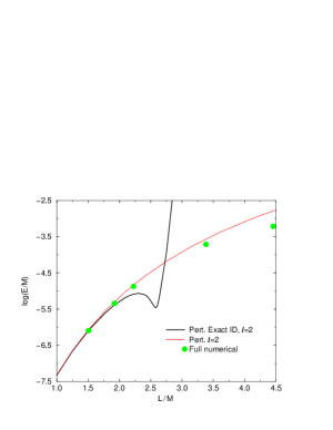
FIG. 1.: The total gravitational radiation computed in the close limit approximation via the Zerilli equation. The solid curve represents the evolution of exact Misner initial data for two equal masses black holes. At the bottom of the dip $(L\approx 2.58)$ the system radiates one order of magnitude less than that predicted by the evolution of linearized initial data (dotted line). For comparison are given the results of full numerical integration of Einstein equations.

IV Curvature perturbations approach

There is an independent formulation of the perturbation problem derived from the Newman-Penrose formalism[4] that fully exploits the null structure of black holes allowing to uncouple for a single wave equation to describe perturbations around Kerr black holes. The outgoing gravitational radiation is fully described in this gauge (and tetrad) invariant formalism by the Weyl scalar

$$\psi_{4}=-C_{\alpha\beta\gamma\delta}\;n^{\alpha}\bar{m}^{\beta}n^{\gamma}\bar{m}^{\delta},$$ (16)

where $n^{\mu}$ and $\bar{m}^{\mu}$ (together with $l^{\mu}$ and $m^{\mu}$) form the tetrad that span the spacetime.

$\psi_{4}$ fulfills the Teukolsky equation, which for the Schwarzschild case reads

$$\ \ \Biggr{\{}\left(-\frac{r^{4}}{\Delta}\right)\partial_{tt}+4r\left(1-\frac{Mr}{\Delta}\right)\partial_{t}$$ (18)

$$\ \ +\,\Delta^{2}\partial_{r}\left(\Delta^{-1}\partial_{r}\right)+\frac{1}{\sin\theta}\partial_{\theta}\left(\sin\theta\partial_{\theta}\right)+\left(\frac{1}{\sin^{2}\theta}\right)\partial_{\varphi\varphi}$$

$$-\left[\frac{4i\cos\theta}{\sin^{2}\theta}\right]\partial_{\varphi}-\left(4\cot^{2}\theta+2\right)\Biggr{\}}r^{4}\psi_{4}=0,$$ (19)

where $\Delta=r^{2}-2Mr$.

The first step towards building up the initial $\psi_{4}$ and $\partial_{t}\psi_{4}$ is to find an instantaneous exact tetrad compatible with the data (1). We have found it by choosing the $l^{\mu}$ and $n^{\mu}$ that generate shear free null congruences (spin coefficients $\sigma=0=\lambda)$ and fix the form of $m^{\mu}$ and its complex conjugate $\bar{m}^{\mu}$ under transformations of type III (boosts) in such a way that the spin coefficient $\epsilon=0$. Our tetrad is then

$$(l^{\mu}) = \bigg{(}\frac{1}{1-2M/r},\Phi^{-2},0,0\bigg{)}\;,$$ (20)

$$(n^{\mu}) = \frac{1}{2}\,\bigg{(}1,-(1-2M/r)\Phi^{-2},0,0\bigg{)}\;,$$ (21)

$$(m^{\mu}) = \frac{\Phi^{-2}}{\sqrt{2}r}\,\bigg{(}0,0,1,i/\sin\theta\bigg{)}\;.$$ (22)

Using formulae (3.1) and (3.2) of Ref. [12] that give $\psi_{4}$ and $\partial_{t}\psi_{4}$ in terms of the 3-geometry and the extrinsic curvature (here vanishing) we obtain

$$\psi_{4}\Big{|}_{t=0}=\frac{(1-2M/r)}{2r^{2}\Phi^{6}}\left\{-3(\partial_{\theta}\Phi)^{2}+\Phi(\partial^{2}_{\theta}-\cot\theta\ \partial_{\theta})\Phi\right\}$$ (23)

(24)

$$\partial_{t}\psi_{4}\Big{|}_{t=0}=-\frac{2M}{r^{2}\Phi^{2}}\psi_{4}\Big{|}_{t=0}\;.$$ (25)

The evolution of this initial data via the Teukolsky equation [13] produce the results shown in Fig. 2 for the total energy emitted as gravitational waves. There is no dip at any value of the separation of the holes. The predicted energy agrees with the full numerical results for all $\mu_{0}<1.8$. For larger values of the separation (although we evolved here exact initial data for two distinct black holes) we overestimate the radiated energy at practically the same rate as the original Price–Pullin result who extrapolated the linearized, $\ell=2$, initial data to values of $(\mu_{0}>1.58)$ beyond the radius of convergence of their expansion parameter, i.e. $M\coth(\mu_{0})/(4R\Sigma_{1})>1$. Correcting for this fact produce the $\ell=2$ piece of the curve labeled as “Linear”.

FIG. 2.: The total radiated energy as computed using the Newman-Penrose-Teukolsky approach. The solid line is the linear evolution of the exact initial data for two black holes initially at rest. There is complete agreement with full numerical results for $L<3.3$ and with the Price-Pullin results (labeled as PP, $\ell=2$) all the way up to much bigger initial separations, keeping under control all the initial nonlinearities. Also shown two other notions of perturbative initial data in the Newman-Penrose formalism.

How robust is this result? To answer this question we fist considered different tetrad rotations of type III to define the relative normalization of the vectors $l^{\mu}$ and $n^{\mu}$ while keeping fixed its null directions. The total radiated energy was quite insensitive to this choice. Some choices slightly improved the agreement with full numerical results, but we found not a priori justification for such choices. We thus keep tetrad (20), which in the Schwarzschild limit reproduces the background tetrad[4] used to write down the Teukolsky equation in Boyer–Lindquist coordinates.

We also essayed two possible definitions of perturbative notion in the Newman–Penrose formalism. The first one, that we called perturbative, considers the exact Weyl tensor contracted with the background (Schwarzschild) tetrad

$$\psi_{4}^{\rm pert}\Big{|}_{t=0} = \frac{(1-2M/r)(1+\Phi^{4})}{4r^{2}\Phi^{2}}$$ (27)

$$\times\left\{-3(\partial_{\theta}\Phi)^{2}+\Phi(\partial^{2}_{\theta}-\cot\theta\ \partial_{\theta})\Phi\right\}$$

$$\partial_{t}\psi_{4}^{\rm pert}\Big{|}_{t=0} = -\frac{4M}{r^{2}(1+\Phi^{4})}\psi_{4}\Big{|}_{t=0}\;,$$ (29)

and a second possibility, that we called linear because it considers only linear terms in the conformal factor $\Phi$, gives

$$\psi_{4}^{\rm linear}\Big{|}_{t=0} = \frac{(1-2M/r)}{2r^{2}}\left(\partial^{2}_{\theta}-\cot\theta\ \partial_{\theta}\right)\Phi$$ (30)

$$\partial_{t}\psi_{4}^{\rm linear}\Big{|}_{t=0} = -\frac{2M}{r^{2}}\psi_{4}\Big{|}_{t=0}\;.$$ (32)

The resulting energy is essentially unchanged in the $\mu_{0}<1.8$ regime and grows steeper than the exact initial data for larger initial separations of the holes. This is because for the initial perturbative $\psi_{4}$’s higher $\ell$ contributions are less under control than for the exact initial $\psi_{4}$. This is seen in the waveforms extracted far away from the system. While for the perturbative choices of $\psi_{4}$ waveforms look fine up to $\mu\approx 1.6$ those evolved from the exact $\psi_{4}$ reach $\mu\approx 2.0$ without much higher $\ell$ content. No dip was found at any value of the separation of the holes and in fact we could not reproduce Fig. 1 results within the Newman-Penrose-Teukolsky formalism. This gives us a measure of a certain robustness of this approach against nonlinearities included in the initial data.

V A closer look at the problem

Since both evolution equations, Zerilli’s and Teukolsky’s are equivalent in the linear perturbations regime we are working in, the different results obtained must be related to how $\psi_{4}$ and $Q$ handle the nonlinearities included in the Misner data. We then first plot in Fig. 3 the Moncrief waveform normalized to $\kappa_{2}$ such that in the linear regime all curves would superpose. Still for $\mu_{0}=1.0$ the curve do not deviate much from that of the linear data. As we increase the initial separation of the holes we find an steady increase of the amplitude in the region $r^{*}<0$ while for $r^{*}>0$ the curves lie on top of each other. Most of the outgoing radiation is generated around the top of the Zerilli potential $V_{\ell}$ at $r^{*}/2M\approx 0.95$. The form of the initial data in terms of $Q_{\ell}$ do not show any particular feature around $\mu_{0}=1.41$. Their relative form continues to grow in amplitude very close to the horizon, but remains almost unchanged further outside. We checked that the effect of the change of the expansion parameter at $\mu_{0}=1.56865$ described above is not responsible for the dip at $\mu_{0}=1.41$.

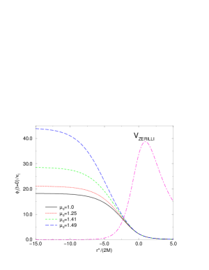
FIG. 3.: The $\ell=2$-multipole projection of the exact Misner data is used to build up the Moncrief-Zerilli initial waveform. Waveforms are normalized by $\kappa_{2}$ in order to show only deviations from the linear regime. Also shown is the Zerilli potential to stress that initial data only differ well inside the potential barrier.

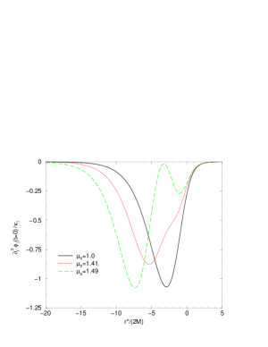
FIG. 4.: The initial second time derivative of the Moncrief waveform normalized by $\kappa_{2}$ to compare with the linear initial data. While there is a good superposition of data form $r^{*}>0$, notable differences appear for $r^{*}<0$. the maximum amplitude decreases steadily for $0<\mu_{0}<1.41$ and increases for $\mu_{0}>1.41$. Also the location of the maximum amplitude monotonically recedes towards more negative $r^{*}$ as $\mu_{0}$ increases. This provokes a decrease of the frequency for which destructive interference of the outgoing radiation occurs.

The quantity directly related to radiation $\partial_{t}Q$ initially vanishes for Misner data (time symmetric), in Fig. 4 we plot thus $\partial_{t}^{2}Q$ at $t=0$. Observe again the good superposition for $r^{*}>0$. There is also a big depression for linear data with a minimum at $r^{*}/2M\approx-3$. As the two black holes start more separated and $\mu_{0}$ increases, the amplitude of this depression decreases and its location recedes towards more negative $r^{*}$’s. This continues so until we reach $\mu_{0}\approx 1.41$. Then the amplitude begins to grow while still the location of the depression recedes towards negative $r^{*}$’s. Is this relatively small decrease of the amplitude (around 20%) responsible for one order of magnitude less radiated energy? Actually since the depression is located very close to the horizon, well inside the potential barrier, most of the radiation generated is swallowed by the black hole and just a very small piece of it reaches infinity. To answer the above question one has to take into account the wave nature of the gravitational radiation. We know that a great deal of the radiation coming out to infinity is generated around the maximum of the Zerilli potential at $r^{*}_{max}/2M\approx 0.95$. There will also be a piece of the disturbance generated at around the pick of $\partial_{t}^{2}Q$. these two pulses will be out of phase by $(2M\omega)(\Delta t/2M)$ where $\Delta t$ is the time the pulse generated close to the horizon takes to arrive at $r^{*}/2M\approx 0.95$. Depending on their relative phases these two pulses can produce constructive or destructive interference. Assuming $\Delta t\sim\Delta r^{*}$, where $\Delta r^{*}$ is the distance between the pick of $\partial_{t}^{2}Q$ and the maximum of the Zerilli potential. In the linear regime, this analysis show that the destructive interference appears for frequencies $2M\omega>1.2$; too high to influence the total energy radiated at infinity. As we increase $\mu_{0}$, the pick in Fig. 4 moves to the left, thus generating destructive interference at lower frequencies. In Fig. 5 we show that this effect is clearly visible in the three spectra for $\mu_{0}=1.38,\ 1.41,\ 1.45$. There is destructive interference around $2M\omega\approx 0.95,\ 0.83,\ 0.65$ respectively. The strong suppression of the radiation at $\mu_{0}=1.41$ is then due to destructive interference right at the frequency of the maximum of the linear spectrum, at $2M\omega\sim 0.8$.

By the same mechanism we can explain the sudden increase in the radiated energy for $\mu_{0}>1.4$. It is now the effect of destructive interference acting at too low frequencies and constructive interference at higher ones together with a dramatic increase of the amplitude of the initial data with respect to the linear regime. Finally for $\mu_{0}>1.56865$ the effect of the change in the perturbative parameter makes things blow up.

FIG. 5.: The spectrum of the gravitational radiation far away from the system as evolved by the Zerilli equation. The solid line labeled with the separation parameter $\mu_{0}=1$ gives essentially the linear regime (we rescaled its amplitude by one fifth). we see how the suppression effect sets up sharply around $\mu_{0}=1.41$. For $\mu_{0}=1.38,\ 1.41,\ 1.45$ destructive interference occurs around frequencies $2M\omega\approx 0.95,\ 0.83,\ 0.65$ respectively.

Alternatively one can look at the initial form of $\psi_{4}$ and its time derivative computed via the linear transformations given in Refs. [5, 6] in terms of the initial Moncrief waveform $\psi$. This transformation can be seen as part of the process of linearization that takes place during the evolution with the Zerilli equation. We observe then in Fig. 4 the same receding of the picks as the initial separation of the holes increase, and its separation from the maximum of the Zerilli potential agrees very well with the prediction coming from the interference patterns seen in Fig. 5. We will see that this behavior is in contrast with that of the direct computation of the exact $\psi_{4}$ and $\partial_{t}\psi_{4}$.

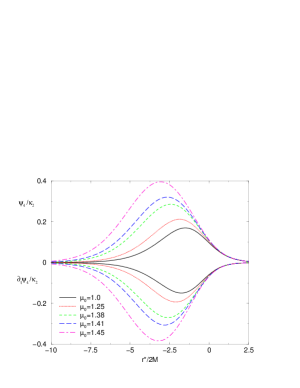
FIG. 6.: Initial $\psi_{4}$ and $\partial_{t}\psi_{4}$ derived from the Moncrief waveform $\phi_{2}$ via Eq. (2.9) of Ref. [6] for different initial separations of the holes.

VI Discussion

Unraveled the mechanism that generates the Abrahams –Price dip, there remains the question of why nothing like this happens when we use the Newman–Penrose–Teukolsky approach to Schwarzschild perturbations. Again, a plot of the initial data for different separations leads to the answer. In Fig. 7 we observe that the maximum of the initial data for increasing $\mu_{0}$ shifts toward increasing $r^{*}$’s instead of more negative ones as happened for the Zerilli formalism. Thus regardless of a small decrease in the amplitude the destructive interference occurs at too high frequencies to influence the outgoing radiation.

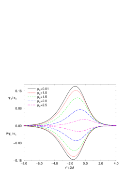
FIG. 7.: The exact initial $\psi_{4}$ and $\partial_{t}\psi_{4}$ for the Misner geometry. The effect of increasing $\mu_{0}$ is to decrease the amplitude and shift the maximum towards less negative $r^{*}$. Curves tend to superpose in the region more relevant for radiation, $r^{*}>0$.

The study of exact initial data evolved linearly has taught us several lessons: i) How the initial Misner data vary with respect to their linearized version and which aspects of them are relevant for computation of the gravitational radiation that reaches infinity. ii) The interference effects that occurs when one evolve these initial data. Note that the occurrence of interference is in general independent of nonlinearities. In fact it is rather sensitive to the shift of the maximum that they produce in the particular case of Misner data. iii) Since the Zerilli–Moncrief waveform and $\psi_{4}$ are two intrinsically different objects, they respond differently to nonlinearities. We have seen that for the initial data studied in this paper $\psi_{4}$ is a better suited quantity to evolve linearly.

There is still another way of evolving Misner data. namely nonlinearly, by direct full numerical integration of Einstein equations. In this way we of course evolve nonlinear initial data and obtain the correct behavior. In Ref. [14] we used the code Cactus to evolve the full set of Einstein equations for a single distorted black hole. We have found that even for small linear initial distortions we needed to solve the initial value problem nonlinearly, otherwise errors in satisfying the constraints would generate numerically unstable evolutions.

Our results are relevant to the idea of evolving fully numerically binary black holes starting from large separations (starting from Post-Newtonian initial data) until a common horizon encompasses the system and then let perturbation theory to take over[7]. The perturbation taking over full numerical method has the advantage of optimizing supercomputer resources, concentrating them in the region where the two black holes are completely detached and full nonlinear relativistic effects take place. Once a common horizon forms one can assume the close limit approximation to hold and continue the evolution with a single wave equation on the background of a Kerr black hole. It is very fortunate that is the Newman-Penrose-Teukolsky approach rather than the Regge-Wheeler-Zerilli one that has this nice behavior in response to nonlinear Cauchy data since the Teukolsky equation can be generalized to rotating black hole backgrounds while the metric perturbation approach do not. Unless there is a dramatic progress in full numerical technics, this perturbative–full numerical hybrid, is our only chance to get waveform templates for inspiraling black holes before laser interferometers begin to operate. The effect described in Fig. 1 inhibit us from using the Zerilli equation to that end. On the other hand, the Teukolsky evolution seems better suited for this marriage between full numerical and perturbative approaches. We also checked that the same general bad behavior of the Zerilli equation and healthy one for the Teukolsky equation holds when one considers Brill-Lindquist initial data (other solution of the conformally flat, time symmetric initial value problem). If this behavior is also true in the astrophysically more appealing scenario of orbiting black holes is currently under investigation. If we remain within the Bowen–York family of initial data (conformally flat and Longitudinal) we expect a decomposition of the conformal factor of the type[15] $\Phi=\Phi_{Misner}+\Phi_{reg}$, where $\Phi_{reg}$ is proportional to the square of the momentum of the holes and the square of their distance. This means that at least for black holes with small initial momentum the effects discussed in this paper should qualitatively still be present.

Another situation where our results should be considered is when one is interested in studying second order perturbations of rotating black holes[16]. The perturbative approach to the Newman-Penrose formalism form a hierarchy of equations

$$\widehat{{\cal T}}\psi_{4}^{(N)}={\cal S}[\psi^{(N-1)},\partial_{t}\psi^{(N-1)}].$$ (33)

where ${\cal T}$ stands for the background wave operator of the Teukolsky equation, $\psi_{4}^{(N)}$ is the waveform of the $N$ perturbative order considered, and ${\cal S}$ is a source term formed by products of all perturbations of order lower than $N$.

One can solve the above equations by evolving initial data order-by-order, successively reaching the next perturbative stage. An alternative approach to that is to evolve exact initial data with the first order wave equation (it has a vanishing source term in vacuum), and then evolve second order equations with vanishing initial data (expressing the source in terms of the first order perturbations). This is consistent to the desired second perturbative order. The justification to this approach can be found from a Laplace transform analysis. In the appendix of paper [5] it is explicitly found that the initial data dependence can be included in the Teukolsky equation as an additional source term, ${\cal S}_{ID}$ and this holds at each order $N$ in the above hierarchy of equations (33). Since the additional source term adds linearly and the wave operator is always the background one, summing over all $N$ orders corresponds to evolve the first order equation with the exact initial data. Then one evolves all higher orders with vanishing initial data.

- [1] R.H. Price and J. Pullin, Phys. Rev. Lett. 72, 3297 (1994).
- [2] J. Pullin, in the Proceedings of the GR15, N. Dadhich and J. Narlikar Eds., Inter-Univ. Centre for Astr. and Astrop., Puna (1998), p87.
- [3] A. Abrahams and R. H. Price, Phys. Rev. D53, 1963 (1996).
- [4] S.A. Teukolsky, Astrophys. J. 185, 635 (1973).
- [5] M. Campanelli and C.O. Lousto, Phys. Rev. D 58, 024015 (1998).
- [6] M. Campanelli, W. Krivan and C. O. Lousto, Physical Review, D58, 024016 (1998).
- [7] M. Alcubierre, J. Baker, B. Brügmann, M. Campanelli, D. Holz, C. Lousto, E. Seidel, R. Takahashi, “The Lazarus project” (unpublished).
- [8] C. W. Misner, Ann. of Phys. 24, 102 (1963); R. W. Lindquist, J. Math. Phys. 4, 938 (1963).
- [9] V. Moncrief, Ann. Phys. (NY) 88, 323 (1974).
- [10] C.O. Lousto and R.H. Price, Phys. Rev. D 55, 2124 (1997).
- [11] P. Anninos, D. Hobil, E. Seidel, L. Smarr, and W.-M. Suen, Phys. Rev. D 52, 2044 (1995).
- [12] M. Campanelli, C.O. Lousto, J. Baker, G. Khanna and J. Pullin, Phys. Rev. D 58, 084019 (1998)
- [13] W. Krivan, P. Laguna, P. Papadopoulous and N. Anderson, Phys. Rev. D 56, 3395 (1997).
- [14] S.Brandt, J. Baker, M. Campanelli, C. Lousto, E. Seidel, and R. Takahashi, “Nonlinear and Perturbative Evolution of Distorted Black Holes. II. Odd-parity Modes”, preprint AEI-1999-7 and gr-qc/9911013.
- [15] C.O. Nicasio, R.J. Gleiser, R.H. Price and J. Pullin, Phys. Rev. D59, 044024 (1999).
- [16] M. Campanelli and C.O. Lousto, Phys. Rev. D 59, 124022 (1999).