Cosmic implications on thermodynamics
and the explanation of the so called horizon problem

Abstract

We show that there are implications on thermodynamics that come from the existence of the initial cosmic singularity. At present time this is more a conceptual change than an observable one. However at very early cosmic times there is a big difference between the actual behavior of thermodynamic quantities and the behavior assumed in the standard cosmological model. We present the discussion of two systems: an ideal monatomic gas at present, and a photon gas at the early Universe. We show the striking result that the entropy density goes to zero as the cosmic time goes to zero. This in turn, provides an explanation for the so called horizon problem.

When one studies a thermodynamic system one normally have the thermodynamic laws, resting on our knowledge of the phenomenological equations of state; and one also seeks for an explanation of all these laws from statistical mechanics. If for example we study a simple system like a classical ideal monatomic gas composed of $N$ molecules in a volume $V$ at temperature $T$; we have the phenomenological thermodynamic description in terms of the equations of state for the pressure $P$ and the internal energy $U$; namely $P_{{\em Ph}}=(Nk_{B}T)/V$ and $U_{{\em Ph}}=\frac{3}{2}Nk_{B}T$[1]; where $k_{B}$ is Boltzmann’s constant and we are using the subscript _Ph to emphasize that these expressions have a phenomenological origin. One also has the explanation of these equations from a microscopical description from statistical mechanics. In the process of performing a calculation in the framework of statistical mechanics, one needs to settle the appropriate distribution of probabilities for the microscopic states. This distribution is normally calculated from the maximum entropy principle[1][2]; which basically states that the probabilities $p_{i}$ for the system to be in the microscopic state $i$ is to be calculated by maximizing the entropy $S(U,V,N)$ subject to the information that we have on the system. For example in the above case of the classical ideal gas, one would say that while the volume $V$ and the number of molecules $N$ are fixed; we only know for the microscopic energy that its average value must coincide with $U$; that is, $\sum p_{i}E_{i}=U$; since the fact that our system is at temperature $T$, precludes us from a more precise information on the energy of the system. Therefore to calculate the distribution of probabilities $\left\{p_{i}\right\}$ we must maximize the entropy

$$S=-k_{B}\sum p_{i}\ln p_{i}$$ (1)

subject to the condition

$\displaystyle\sum p_{i}E_{i}=U.$

The distribution so obtained is given by:

$$p_{i}=\frac{e^{-\beta E_{i}}}{\sum_{j}e^{-\beta E_{j}}},$$ (2)

where $\beta=1/(k_{B}T)$; which is recognized as the Gibbs or canonical distribution.

We have said before that the entropy must be maximized subject to the information that we have on the system; and we do want to take into account that we live in a Universe with an initial cosmic singularity. The way in which this observation affects our statistical mechanic calculation is by imposing some constrains on the available phase space of our system. More precisely, the existence of an initial cosmic singularity implies that there are particle horizons[3]; which means that our past and the amount of matter that we can observe are finite. The implication of this is that we can not assume that our thermodynamic system is in contact with an infinite reservoir at temperature $T$. In particular this means that not all of the theoretically predicted energy levels $E_{j}$ are available; since, if we label with $E_{\max}$ the total available energy in our causal past, then clearly we can only consider $E_{j}\leq E_{\max}$.

Following the standard calculation for a classical ideal gas[1] we find that the partition function $Z=\sum_{j}e^{-\beta E_{j}}$, appearing in the denominator of (2) above, is given by

$$Z=\sum_{j,j\prime,j\prime\prime,...}e^{-\beta\left(\varepsilon_{1j}+\varepsilon_{2j\prime}+\varepsilon_{3j\prime\prime}+...\right)};$$ (3)

where $\varepsilon_{ij}$ is the energy of the particle $i$ in the state $j$. In the usual presentation of a classical ideal gas, it is assumed non-interaction and statistical independence for each atom of the gas; from which it is deduced that the sums over each of the indices appear as factors; so that the partition function would be given by $Z=z^{N}/N!$, where $z$ is given, in the continuous representation, by

$$z=\frac{V}{h^{3}}\int e^{-\beta\frac{p^{2}}{2m}}dp_{x}dp_{y}dp_{z};$$ (4)

where $h$ is Planck constant. The correcting factor $1/N!$, accounts for the indistinguishability of the particles[1][2].

Due to the restriction on the phase space coming from our cosmological knowledge we are not free to integrate in (4) up to arbitrary large values of $p^{2}$; since $\frac{p^{2}}{2m}$ can not be larger that the total available energy $E_{\max}$ in our causal past; in other words we must have $\frac{p^{2}}{2m}\leq E_{\max}$. Therefore, one has $z=\frac{\pi V}{h^{3}}\sqrt{2^{5}\left(m/\beta\right)^{3}}\int_{0}^{\beta E_{\max}}e^{-x}x^{1/2}dx$. In the limit for $E_{\max}$ going to infinity one obtains the usual result $z_{\infty}=(V/h^{3})(2\pi mk_{B}T)^{3/2}$; however due to the cosmological restriction we can show that

$$\ln Z(\beta,V,N) = N\ln\left(\frac{\pi V}{h^{3}}\sqrt{2^{5}\left(m\right)^{3}}\right)-\frac{3}{2}N\ln\beta$$

$$+N\ln\int_{0}^{\beta E_{\max}}e^{-x}x^{1/2}dx-\ln N!\quad.$$

Then the entropy is given by

$\displaystyle S=k_{B}\beta\sum\frac{e^{-\beta E_{i}}}{Z}E_{i}+k_{B}\ln Z=k_{B}\beta U+k_{B}\ln Z.$

And the corresponding energy is given by

$$U=Nk_{B}T\left(\frac{3}{2}-\frac{x_{c}^{3/2}e^{-x_{c}}}{\int_{0}^{x_{c}}e^{-x}x^{1/2}dx}\right)$$ (5)

with $x_{c}\equiv\beta E_{\max}$. To give an idea of the order of magnitude of the correcting term, let us consider $T=300{{}^{\circ}}{\rm K}$, and a cosmic mass density $\rho$ to be two percent of the critical mass density; that is, $\rho=0.02\rho_{c}=(0.02)3H_{0}^{2}/8\pi G$, with the Hubble parameter $H_{0}$ with value $H_{0}=75(km/s)/Mpc$; and where $G$ is the gravitational constant. Assuming a sphere of radius $R=c/H_{0}$, where $c$ is the velocity of light, one can estimate $E_{\max}$ by $E_{\max}=4\pi R^{3}\rho c^{2}/3$; which implies a value of $x_{c}$ on the order of $x_{c}\simeq 10^{88}$. Such huge value for $x_{c}$ gives a negligible correction in front of $3/2$ in equation (5). Even if one considers temperatures as high as those found in the center of the sun, one will have $x_{c}\simeq 10^{83}$; and the whole correcting term to the equation of state (5), would be of order $10^{-125}$ in front of the $3/2$.

The pressure can be calculated from

$\displaystyle P=\frac{1}{\beta}\frac{\partial\ln Z}{\partial V}=\frac{N}{\beta V};$

therefore in this case the equation of state for the pressure does not show any correction; that is $P=P_{{\em Ph}}$.

It is observed that in the previous expressions the correcting term is more important if $\beta E_{\max}$ becomes smaller. This situation arises when one approaches the initial cosmic singularity; since in this regime $\beta$ goes to zero and also $E_{\max}$ shows the same behavior; due to the fact that the particle horizon reduces its size as one considers earlier cosmic times.

At very early cosmic times, during the radiation dominated era, the different kind of particles contribute to the energy momentum tensor as different components of a relativistic gas. In order to be concrete we will study next the system corresponding to a photon gas in a small volume $V$ at temperature $T$, at very early cosmic times.

The corresponding phenomenological equations of state for this system are: $U_{{\em Ph}}=a\;V\;T^{4}$ and $P_{{\em Ph}}=\frac{1}{3}U_{{\em Ph}}/V\,$; where $a=4\sigma_{0}/c$, and $\sigma_{0}$ is the Stefan-Boltzmann constant. From the knowledge of the equations of state, one can calculate the phenomenological entropy; which is given[1] by $S_{{\em Ph}}=\frac{4}{3}a^{1/4}\;U_{{\em Ph}}^{3/4}\;V^{1/4}$.

In a Friedman Universe the line element is given in terms of the metric of a Robertson-Walker spacetime, namely[4]

$$ds^{2}=dt^{2}-\left(\frac{A(t)}{c}\right)^{2}dl_{k}^{2};$$ (6)

where $A(t)$ is the expansion parameter with units of length and $dl_{k}^{2}$ is the line element of a homogeneous and isotropic space with constant curvature $k=1,0$ or $-1$. In a radiation dominated Universe, $\rho\,A^{4}$ is a constant; and for very early cosmic times, $A(t)$ behaves asymptotically as $\sqrt{t}$; where the initial singularity is attainned in the limit $t\rightarrow 0$. Then, one can deduce that the phenomenological entropy density, $s_{{\em Ph}}\equiv S_{{\em Ph}}(V_{0})/V_{0}$, diverges as $s_{{\em Ph}}\varpropto t^{-\frac{3}{2}}$ when $t\rightarrow 0$.

Let us now proceed with the correct causal statistical mechanic calculation of the entropy, taking into account our knowledge of the initial singularity. As we have seen in the previous example, we expect to find a different expression for the correct entropy; which implies that the corresponding equations of state will be different to those that appear in the standard cosmological model dominated by radiation. This means that to be absolutly consistent one should solve the Einstein equations taking this effect into account. We plan to do this in a future paper; instead here we would like to concentrate in the general behavior of the entropy in a Universe with an initial cosmic singularity, by given the calculation in a fixed geometry. We choose this geometry to be the Friedman line element corresponding to a Universe dominated by radiation. We also have the freedom to relate one of our thermodynamic variables to the geometry; we do this by demanding the energy density to behave as $1/A^{4}$; as it does in the standard cosmological model of a Universe dominated by radiation.

In order to be explicit, let us consider an open Universe; that is, the $k=-1$ case, whose expansion parameter is deterimined from the Friedmann equations[4]

$$A(t)=\left(\frac{\sqrt{Q_{r}}}{c}\right)\sqrt{2\left(\frac{tc^{2}}{\sqrt{Q_{r}}}\right)+\left(\frac{tc^{2}}{\sqrt{Q_{r}}}\right)^{2}},$$ (7)

and where the density $\rho$ is linked to the geometry in such a way that the cuantity $Q_{r}$, defined by $Q_{r}\equiv(8\pi G/3)\rho A^{4}$, is a constant.

Let us consider a reference volume $V_{0}$, which is small enough so that any other dynamical time is much larger than the typical thermodynamic relaxation time[2] associated to our subsystem determined by $V_{0}$. An observer that is comoving with the matter flow ascribes the entropy $S(t)=S(U(t),V_{0})$ to this small subsystem; where the world line of the observer can be parametrized by the cosmic time $t$. Let us recall that the chemical potential for a photon gas is zero; therefore the entropy does not depend on the number of particles.

Following the standard procedures appearing in text books[5] of statistical mechanics one can prove that the entropy and internal energy for electromagnetic radiation contained in a volume $V_{0}$ are given, in the continuum representation, by

$$S = \frac{V_{0}k_{B}}{\pi^{2}c^{3}\beta^{3}\hbar^{3}}\left(\left.-\ln\left(1-e^{-w}\right)\frac{w^{3}}{3}\right|_{0}^{x_{\max}}\right.$$ (9)

$$\left.+\frac{4}{3}\int\limits_{0}^{x_{\max}}\left[\frac{w^{3}}{\left(e^{w}-1\right)}\right]\;dw\right)\,$$

and

$$U=\frac{V_{0}}{\pi^{2}c^{3}\beta^{4}\hbar^{3}}\int\limits_{0}^{x_{\max}}\left[\frac{w^{3}}{\left(e^{w}-1\right)}\right]\;dw\,;$$ (10)

where $x_{\max}(t)=\beta(t)\ E_{\max}(t)$ and the dimensionless variable of integration $w$ is defined by $w=\beta\hbar\omega$.

If there where no particle horizons the first term would not contribute to the value of the entropy; since in this case $x_{\max}=\infty$. Then, in this situation one would reproduce the expression for $S_{{\em Ph}}$ mentioned above.

It is important to remark that the Stefan-Boltzmann law; which gives the energy radiated per second per unit area $I$ for black body radiation, namely, $I=(cU_{{\em Ph}})/(4V)=\sigma_{0}\;T^{4}$, is now corrected by the expression (10). One way to understand this result is that the Stefan-Boltzmann constant $\sigma_{0}$, mentioned above, is actually a parameter that changes with cosmic time; which is given by $\sigma(t)=\frac{k_{B}^{4}}{4\pi^{2}c^{2}\hbar^{3}}\int\limits_{0}^{x_{\max}(t)}\left[\frac{w^{3}}{\left(e^{w}-1\right)}\right]\;dw$; and where one usually approximates for the present time $t_{0}$ by the value $\sigma(t_{0})\backsimeq\sigma_{0}\equiv\frac{k_{B}^{4}}{4\pi^{2}c^{2}\hbar^{3}}\int\limits_{0}^{\infty}\left[\frac{w^{3}}{\left(e^{w}-1\right)}\right]\;dw=\frac{\pi^{2}k_{B}^{4}}{60c^{2}\hbar^{3}}$.

When constructing a cosmological model, one normaly represent matter by some kind of fluid. In any Universe whose energy momentum tensor is that corresponding to a fluid, given an event $p$, one can calculate the total available energy in the causal past of $p$ by integrating the contribution of the fluid on the boundary of the causal past of $p$. In our case we can calculate $E_{\max}(t)$ explicitly by considering the contributions on the past light cone at earlier times $t^{\prime}$ coming from the energy density $\rho(t^{\prime})c^{2}$, with the corresponding red shift factor $A(t^{\prime})/A(t)$ and multiplied by the volume element $4\pi\ r(t,t^{\prime})^{2}A(t^{\prime})\ dl=4\pi\ r(t,t^{\prime})^{2}c\ dt^{\prime}$; where $r(t,t^{\prime})$ is the radius of a sphere, with center at the point of observation at cosmic time $t$, and with surface on the past light cone at time $t^{\prime}$. Considering the realistic case $k=-1$, corresponding to a Universe with energy density below the critical value, the line element of the three dimensional homogeneous and isotropic space can be expressed by $dl^{2}=d\chi^{2}+\sinh(\chi)^{2}(d\theta^{2}+\sin(\theta)^{2}d\phi^{2})$. Using these coordinates, the radius $r(t,t^{\prime})$ of the sphere is given by $r(t,t^{\prime})=A(t^{\prime})\sinh(\chi(t,t^{\prime}))$; where the center of the coordinate system is taken at the point of observation, so that $\chi(t,t)=0$. In the spacetime diagram in Fig. 1 one can see a picture of the coordinate system.

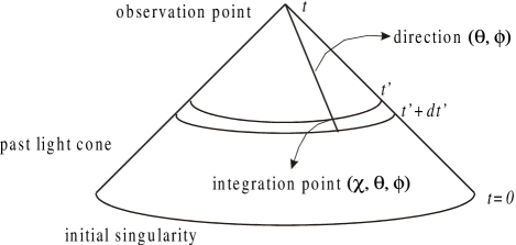
FIG. 1.: The observation point is the tip of the past light cone with the generic time value $t$. A direction of observation with angular coordinates $(\theta,\phi)$ reaches the sphere in the past at time $t^{\prime}<t$, with radial coordinate $\chi$. The past light cone extends up to the initial cosmic singularity with the time value $t=0$.

One can calculate $\chi(t,t^{\prime})$ from the expression $\chi(t,t^{\prime})=c\int_{t^{\prime}}^{t}dt^{\prime\prime}/A(t^{\prime\prime})$; from which it is obtained $E_{\max}(t)$, namely

$$E_{\max}(t) = \int_{0}^{t}\rho(t^{\prime})c^{2}\frac{A(t^{\prime})}{A(t)}4\pi r(t,t^{\prime})^{2}c\ dt^{\prime}$$

$$= \frac{3Q_{r}c^{2}}{4G}\frac{1}{A(\tau)}\left[\left(\tau+1\right)\sqrt{\tau^{2}+2\tau}\right.$$

$$\left.-\ln(\tau+1+\sqrt{\tau^{2}+2\tau})\right];$$

where we are using the convenient dimensionless time variable $\tau=(tc^{2}/\sqrt{Q_{r}})$. In order to study the behavior of $E_{\max}(t)$ near the initial singularity it is useful to express it in terms of $A(\tau)$; which is also a good time variable, since it is a monotonically increasing function of time. In this way one obtains

$$E_{\max} = \frac{3\sqrt{Q_{r}}c^{3}}{4G}\left[\left(\sqrt{\left(\frac{c}{\sqrt{Q_{r}}}A\right)^{2}+1}\right)\right.$$ (12)

$$\left.-\frac{\sqrt{Q_{r}}}{cA}\ln\left(\sqrt{\left(\frac{c}{\sqrt{Q_{r}}}A\right)^{2}+1}+\frac{c}{\sqrt{Q_{r}}}A\right)\right].$$

It is clear that as $t$ decreases, so does the region covered by the particle horizon; and therefore $E_{\max}(t)$ also decreases. More specifically one can show that the asymptotic expression of $E_{\max}$ for small values of $A$ starts with: $E_{\max}(A)=(3\sqrt{Q_{r}}c^{3}/4G)[(2/3)(cA/\sqrt{Q_{r}})^{2}+O((cA/\sqrt{Q_{r}})^{4})]$. In particular, one can see that in the limit $A\rightarrow 0$, one has

$$\lim_{A\rightarrow 0}E_{\max}=0\,.$$ (13)

It should be emphasized that although the energy per unit volume diverges as one approaches the initial cosmic singularity, the maximum possible available energy at any given point is finite, and it goes to zero as $t\rightarrow 0$.

In order to study the behavior of the entropy per unit volume in the vicinity of the initial singularity, we can make an asymptotic expansion of the entropy for very small values of $t$. Defining the entropy density by $s(t)\equiv S(t)/V_{0}$, one obtains

$$s(t) = \frac{k_{B}}{\pi^{2}c^{3}\hbar^{3}}\left(-\frac{E_{\max}(t)^{3}}{3}\ln\left(\beta(t)E_{\max}(t)\right)\right.\,$$ (15)

$$\left.+\frac{4}{9}E_{\max}(t)^{3}\right)+O(\beta(t)E_{\max}(t)^{4}).$$

While in the standard model $\beta(t)$ is given by $\frac{\beta(t_{0})}{A(t_{0})}A(t)$; from our setting one can deduce that actually, $\beta(t)$ must satisfy

$$\beta(t)=\frac{\beta(t_{0})}{A(t_{0})}A(t)\left[\frac{\int\limits_{0}^{\beta(t)\ E_{\max}(t)}\left[\frac{w^{3}}{\left(e^{w}-1\right)}\right]\;dw}{\int\limits_{0}^{\beta(t_{0})\ E_{\max}(t_{0})}\left[\frac{w^{3}}{\left(e^{w}-1\right)}\right]\;dw}\right]^{\frac{1}{4}};$$ (16)

which reduces to the usual behavior when $\beta(t)\ E_{\max}(t)$ and $\beta(t_{0})\ E_{\max}(t_{0})$ are big. Instead, when $\beta(t)\ E_{\max}(t)$ is small, this expression shows a very different behavior for $\beta(t)$. From the fact that $E_{\max}(t)$, for very small $t$, behaves as $A(t)^{2}$, one can deduce from equation (16) that $\beta(t)$ behaves as $A(t)^{10}$, in the vicinity of the initial singularity.

Using both asymptotic behaviors; namely: $E_{\max}(t)\varpropto A(t)^{2}$ and $\beta(t)\varpropto A(t)^{10}$, as $t$ goes to zero, it is easily seen from equation (15) that the entropy density goes to zero when one approaches the initial cosmic singularity; that is

 lim_t→0s(t)=0 . (17)

The consequences of our result regarding the possible initial data for physical fields at the very early Universe, can be better understood if we recall from equation (1) that the entropy is given by $S=-k_{B}\sum\limits_{i}p_{i}\ln p_{i}$; since this expression implies that the only way in which the entropy of a system can go to zero is if all the probabilities $p_{i}$ go to zero except one, let us say $p_{0}$, which must have the unit value. This means that if we where to have two subsystems with identical statistical mechanic description and with zero entropy, then the physical state of both systems would be indistinguishable from the statistical mechanic point of view. This result explains way when we observe the cosmic background radiation in different directions on the sky that where causally disconnected at the time of decoupling, have such a similar description

The attempts to understand the low entropy behavior at the early Universe has been the subject of study from different viewpoints. For example the standard presentations of the postulated inflationary Universes aims to explain the so called horizon problem, which is associated to the low entropy behavior[6].

According to our result we see that there is no problem with the observed initial isotropic and homogeneous behavior of the Universe, regarding the existence of the initial cosmic singularity; since we have seen that such behavior is actually a consequence of the presence of the cosmic singularity.

- [1] H.B. Callen, “Thermodynamics and an introduction to thermostatistics”, second edition, John Wiley & Sons, (1985).
- [2] L.D. Landau and E.M. Lifshitz, “Statistical Physics”, Pergamon Press, (1980).
- [3] W. Rindler, “Visual Horizons in World-Models ”, Mon.Not.Roy.Ast.Soc., 116, 663, (1956).
- [4] R. Wald, “General Relativity”, The Chicago University Press, (1984).
- [5] K. Huang, “Statistical Mechanics”, second edition, John Wiley & Sons.
- [6] A.H. Guth, “Inflationary universe: A possible solution to the horizon and flatness problem”, Phys.Rev.D, 23, 347, (1981).