Eternal inflation and the present universe

Abstract

Eternally inflating universes can contain thermalized regions with different values of the cosmological parameters. In particular, the spectra of density fluctuations should be different, because of the different realizations of quantum fluctuations of the inflaton field. I discuss a general method for calculating probability distributions for such variable parameters and analyze the density fluctuation spectrum as a specific application.

1 Introduction

In this paper I am going to discuss the structure of the universe on super-large scales, so large that we are never going to observe them. I shall argue, however, that this analysis may help us understand some features of the universe within the observable range. This is based on the work done with my student Vitaly Vanchurin at Tufts and with Serge Winitzki at Cambridge University.

Let me begin with a brief introduction to eternal inflation. As we know, inflation is a nearly exponential expansion of the universe,

$$a(t)\approx e^{Ht},$$ (1)

which is driven by the potential energy of a scalar field $\varphi$, called the inflaton. $a(t)$ in Eq.(1) is the scale factor and the expansion rate $H$ is determined by the inflaton potential $V(\varphi)$. Inflation ends when $\phi$ starts oscillating about the minimum of the potential. Its energy is then dumped into relativistic particles and is quickly thermalized.

A remarkable feature of inflation is that generically it never ends completely. At any time, there are parts of the universe that are still inflating [1, 2]. The reason is that the evolution of $\varphi$ is influenced by quantum fluctuations. This appies in particular to the range of $\varphi$ near the maximum of $V(\varphi)$, where the potential is very flat. As a result, thermalization does not occur everywhere at the same time. We can introduce a decay constant $\Gamma$ such that $\tau=1/\Gamma$ is the characteristic time it takes $\varphi$ to get from the maximum to the minimum of the potential. Then the total inflating volume in the universe is proportional to

$${\cal V}_{inf}\propto e^{-\Gamma t}e^{3Ht}.$$ (2)

The first factor on the right-hand side describes the exponential decay of the inflating volume due to thermalization, while the second factor describes the exponential expansion of the regions which still continue to inflate. For flat potentials required for successful inflation, we typically have $\Gamma\ll 3H$, so that ${\cal V}_{inf}$ grows exponentially with time. The thermalized volume grows at the rate $d{\cal V}_{therm}/dt=\Gamma d{\cal V}_{inf}/dt$, and thus ${\cal V}_{therm}$ also grows exponentially.

Different thermalized regions in such eternally inflating universe may have very different properties. Here are some examples.

The potential $V(\varphi)$ may have several minima corresponding to vacua with different physical properties. For example, the values of some constants of Nature (e.g., the electron mass or the cosmological constant) or cosmological parameters (such as the amplitude of density fluctuations, the baryon to entropy ratio, etc.) could be different in the corresponding thermalized regions. A more interesting possibility is that the “constants” are related to some slowly-varying fields and take values in a continuous range. For example, the inflaton could be a complex field, $\varphi=|\varphi|\exp(i\chi)$, with a potential having the shape of a “deformed Mexican hat” (that is, with some $\chi$-dependence). Then different paths that $\varphi$ can take from the top of the potential to the bottom will result in different magnitudes of density fluctuations $\delta\rho/\rho$. The amplitude of the fluctuations will therefore be different in different parts of the universe. Another example is a field $\chi$ (unrelated to the inflaton) with a self-interaction potential $U(\chi)$. If $U(\chi)$ is a very slowly varying function of $\chi$, then it can act as an effective cosmological constant. Quantum fluctuations will randomize $\chi$ during inflation, and observers in different parts of the universe will measure different values of $U(\chi)$.

Perhaps the most important example is the spectrum of cosmological density fluctuations. The density fluctuation $\delta\rho/\rho(l)$ is determined by the quantum fluctuation $\delta\varphi(l)$ of the inflaton field $\varphi$ at the time when the corresponding comoving scale $l$ crossed the horizon. Different realizations of quantum fluctuations $\delta\varphi(l)$ result in different density fluctuations spectra in widely separated parts of the universe. This uncertainty is present in all models of inflation.

In all these examples, we have parameters $\chi$ which we cannot possibly predict with certainty. All we can hope to do is to determine the probability distribution ${\cal P}(\chi)$.

An eternally inflating universe is inhabited by a huge number of civilizations that will measure different values of $\chi$. We can define the probability ${\cal P}(\chi)d\chi$ as being proportional to the number of observers who will measure $\chi$ in the interval $d\chi$ [17]. Now, observers are where galaxies are, and thus ${\cal P}(\chi)d\chi$ is proportional to the number of galaxies in regions where $\chi$ takes values in the interval $d\chi$. We can then write

$${\cal P}(\chi)\propto F(\chi)\nu(\chi),$$ (3)

where $F(\chi)d\chi$ is the fraction of volume in thermalized regions with $\chi$ in the interval $d\chi$, and $\nu(\chi)$ is the number of galaxies per unit volume (as a function of $\chi$). The calculation of $\nu(\chi)$ is a standard astrophysical problem, and here I shall focus on the volume factor $F(\chi)$.

In this discussion I am trying to avoid the word “anthropic”, because it makes some people very upset, but what I want to emphasize is that the approach I have just outlined is as quantitative and predictive as it can possibly be. Once ${\cal P}(\chi)$ is calculated, we can predict, for example, that $\chi$ should have a value in a certain range with 95% confidence.

The first attempts to implement this approach encountered an unexpected difficulty. It can be traced down to the fact that eternal inflation never ends, and the number of galaxies in an eternally inflating universe is infinite at $t\to\infty$. In order to calculate the volume fraction $F(\chi)$, one therefore has to compare infinities, which is an inherently ambiguous procedure. One can introduce a time cutoff and include only galaxies that formed prior to some time $t_{c}$, with the limit $t_{c}\to\infty$ at the end. One finds, however, that the resulting probability distributions are extremely sensitive to the choice of the time coordinate $t$ [4, 5]. Linde, Linde and Mezhlumian [6] attempted to determine the most probable spectrum of density fluctuations using the proper time along the worldlines of comoving observers, which they regarded as the most natural choice of the time coordinate. They found a probability distribution suggesting that a typical observer could find herself at a deep minimum of the density field. On the other hand, if one uses the expansion factor along the worldlines as the time coordinate, one recovers the standard result [7]. Coordinates in general relativity are arbitrary labels, and such gauge-dependence of the results is, of course, an embarrassment.

The rest of the paper is organized as follows. After reviewing the physics of eternal inflation in Section 2, I discuss the spacetime structure of an eternally inflating universe in Section 3. This will help us understand the origin of the gauge-dependence problem. The proposed resolution of the problem is discussed in Section 4. As a specific application, the spectrum of density fluctuations measured by a typical observer is analyzed in section 5. The conclusions are briefly summarized in Section 6.

2 Eternal inflation

The metric of an inflating universe has a locally Robertson-Walker form,

$$ds^{2}=dt^{2}-a^{2}(t)d{\bf x}^{2},$$ (4)

with the expansion rate given by

$${\dot{a}}/a\approx H(\varphi)=[8\pi V(\varphi)/3]^{1/2}.$$ (5)

The potential $V(\varphi)$ is assumed to be a slowly varying function of $\varphi$. As a result, $H$ is a slowly varying function of the coordinates, and we have an approximately de Sitter space with a horizon distance $H^{-1}$. The classical slow-roll evolution equation for $\varphi$ is

$${\dot{\varphi}}_{cl}\approx-H^{\prime}(\varphi)/4\pi.$$ (6)

Quantum fluctuations of $\varphi$ can be represented as a random walk with random steps taken independently in separate horizon-size regions, with one step per Hubble time $H^{-1}$. The rms magnitude of the steps is

$$\delta\varphi_{rms}=(H/2\pi).$$ (7)

We do not have a completely satisfactory derivation of this stochastic picture in the general case. Its main justification is that it reproduces the results of quantum field theory in de Sitter space for a free scalar field of mass $m\ll H$ (that is, the two-point function obtained by averaging a classical stochastic field coincides with the quantum two point function). For flat inflaton potentials, the dynamics of $\varphi$ should be close to that of a free field, so one expects the stochastic picture to apply with a good accuracy.

Let us define the distribution $F(\varphi,t)d\varphi$ as the volume occupied by $\varphi$ in the interval $d\varphi$ at time $t$. It satisfies the Fokker-Planck equation [1, 8, 9, 10, 11, 4]

$$\partial_{t}F+\partial_{\varphi}J=3H^{\alpha}F,$$ (8)

where

$$J=-{1\over{8\pi^{2}}}\partial_{\varphi}(H^{\alpha+2}F)-{1\over{4\pi}}H^{\alpha-1}H^{\prime}F.$$ (9)

The first term of the flux $J$ describes quantum “diffusion” of the field $\varphi$, while the second term corresponds to the classical “drift” described by Eq.(6). The parameter $\alpha$ in Eqs.(8),(9) represents the freedom of time parametrization, with the time variable $t$ related to the proper time $\tau$ according to $dt=H^{1-\alpha}d\tau$. Hence, $\alpha=1$ corresponds to the proper time, $t=\tau$, and $\alpha=0$ to the scale factor time, $t=\ln a$.

A great deal of research has been done on the properties of the Fokker-Planck equation (8) and on its solutions. To summarize the conclusions, there are some good news and some bad news. The good news is that the asymptotic form of the solutions of (8) is

$$F(\phi,t)\to F(\phi)e^{\gamma t}~{}~{}~{}~{}~{}~{}~{}(t\to\infty).$$ (10)

The overall factor $e^{\gamma t}$ drops out in the normalized distribution, and thus one gets a stationary asymptotic distribution for $\varphi$. The bad news is that $F(\varphi)$ has a strong dependence on $\alpha$, so that the results are very sensitive to the choice of the time coordinate [4]. This is a very disturbing conclusion, and one could have thought that there is something wrong with the Fokker-Planck equation (8). We shall see, however, that there is a good physical reason for the gauge-dependence of $F(\varphi)$, so the equation is not to blame.

3 Spacetime structure of an eternally inflating universe

To analyze the spacetime structure of an eternally inflating universe, one can perform numerical simulations using the stochastic representation of quantum fluctuations [12, 4]. Here, I present the results of the simulations performed by V. Vanchurin, S. Winitzki and myself [13]. We consider a comoving region which has a horizon size $l=H^{-1}$ and a homogeneous inflaton field $\varphi=0$ at the initial moment $t=0$. We evolve $\varphi$ in time increments $\delta t$ according to the rule

$$\delta\varphi({\bf x})={\dot{\varphi}}_{cl}({\bf x})\delta t+\delta\varphi_{q}({\bf x}),$$ (11)

where ${\dot{\varphi}}_{cl}$ is from Eq.(6) and $\delta\varphi_{q}({\bf x})$ is a random Gaussian field of zero mean,

$$\langle\delta\varphi_{q}({\bf x})\rangle=0,$$ (12)

and with a correlation function

$$\langle\delta\varphi_{q}({\bf x})\delta\varphi_{q}({\bf x^{\prime}})\rangle=\left({H\over{2\pi}}\right)^{2}(H\delta t)C(r).$$ (13)

Here, $r$ is the physical distance between the points ${\bf x}$ and ${\bf x^{\prime}}$, $C(0)=1$, and $C(r)$ rapidly drops to zero at $r\gg H^{-1}$. The correct asymptotic form is $C(r)\propto r^{-4}$ [14]; in the simulations we set $C(r)=0$ for $r>2H^{-1}$. The scale factor $a({\bf x},t)$ is evolved according to

$$\delta a({\bf x})=H({\bf x})a({\bf x})\delta t.$$ (14)

The spatial distribution of inflating and thermalized regions in a $(2+1)$-dimensional simulation is shown in Fig.1. We used a double-well potential for the inflaton,

$$V(\varphi)=V_{0}\cos^{2}(\kappa\varphi),$$ (15)

where $\kappa=\pi/2\eta$, and we only consider the range $-\eta<\varphi<\eta$. Inflating regions are white, and the two types of thermalized regions corresponding to the minima at $\varphi=\pm\eta$ are shown with different shades of grey. As time goes on, larger and larger fraction of the comoving volume gets thermalized, so the inflating regions shrink in comoving coordinates. The inflating regions can be thought of as inflating domain walls separating the two types of vacua. Since the domain walls cannot disappear for topological reasons, it is clear that inflation must be eternal in this model [15].

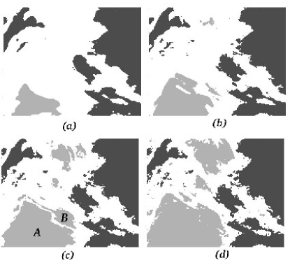
Figure 1: A two-dimensional simulation for the double-well model at four consecutive moments of time [13]. We evolved a comoving region of initial size $l=H^{-1}$ with the initial value of $\phi=0$. Inflating regions are shown white, while thermalized regions with $\phi=+\eta$ and $\phi=-\eta$ are shown with different shades of grey. Thermalized regions of the same type can join in the course of the simulation. For example, regions labeled $A$ and $B$ in snapshot (c) have merged into a single region in snapshot (d). However, regions of different types cannot merge: they are separated by inflating domain walls.

The spacetime structure of the universe in these simulations is illustrated in Fig.2. Now, the vertical axis is time and the horizontal axis is one of the spatial directions. The boundaries between inflating and thermalized regions, which play the role of the big bang for the corresponding thermalized regions, are infinite spacelike surfaces. In the figure, these boundaries become nearly vertical at late times, so that they appear to be timelike. The reason is that the horizontal axis in Fig.2 is the comoving distance, with the expansion of the universe factored out. The physical distance is obtained by multiplying by the expansion factor $a(t)$, which grows exponentially as we go up along the time axis. If we used the physical distance in the figure, the thermalization boundaries would “open up” and become nearly horizontal (but then it would be difficult to fit more than one thermalized region in the figure).

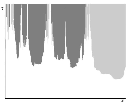
Figure 2: Spacetime structure in a one-dimensional simulation for the double-well model. It can be thought of as a spacetime slice through the $(2+1)$-dimensional simulation illustrated in Fig.1. The shading code is the same as in Fig.1.

Thermalization is followed by a hot radiation era and then by a matter-dominated era during which luminous galaxies are formed and civilizations flourish. All stars eventualy die, and thermalized regions become dark, cold and probably not suitable for life. Hence, observers are to be found within a layer of finite (temporal) width along the thermalization boundaries in Fig.2.

It is now easy to see why the probability distributions obtained using a cutoff at $t=t_{c}$ are so sensitive to the choice of the time variable $t$. Any spacelike surface ${\cal S}$ can be an equal-time surface $t=t_{c}$ with an appropriate choice of $t$. Depending on one’s choice, the surface ${\cal S}$ may cross many thermalized regions of different types (e.g., for $t=\tau$), may cross only regions of one type, or may cross no thermalized regions at all (say, for $t=\varphi$ with $\varphi$ in the deterministic slow-roll range). These possibilities are illustrated in Fig.3 by surfaces ${\cal S}_{1},{\cal S}_{2}$ and ${\cal S}_{3}$, respectively. If, for example, one uses the surface ${\cal S}_{2}$ as the cutoff surface, one would conclude that all observers will see the same vacuum with 100% probability. With a suitable choice of the surface, one can get any result for the relative probability of the two minima.

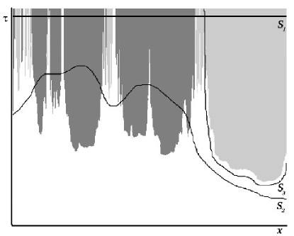
Figure 3: ${\cal S}_{1}$ is a surface of a constant proper time. It crosses many thermalized regions of different types. ${\cal S}_{2}$ is a spacelike surface which crosses regions of only one type. ${\cal S}_{3}$ is a spacelike surface which does not cross any thermalized regions.

We have also performed simulations for a two-field model with a potential

$$V(\varphi,\chi)=V_{0}\cos^{2}(\kappa\varphi)[1+\lambda(1+\cos\beta\chi)\sin^{4}\kappa\varphi],$$ (16)

where $V_{0},\kappa,\beta$ and $\lambda$ are constants. We start the simulation in a horizon-size region with $\varphi=\chi=0$ at the initial moment $t=0$. A spacetime slice through one of the simulations is given in Fig.4, where different values of $\chi$ are shown with different shades of grey in the inflating regions, while the thermalized regions are left white. The field $\chi$ is homogeneous at the bottom of the figure ($t=0$), but gets randomized by quantum fluctuations as time goes on. Different regions of space thermalize with different values of $\chi$, and $\chi$ takes all of its values on each thermalization surface. It is clear that the simple explanation of gauge-dependence that I gave for the one-field model, that constant-$t$ surfaces can be chosen so that they cross one type of thermalized regions and avoid the other, does not apply in this case. For the two-field model, the situation is more subtle.

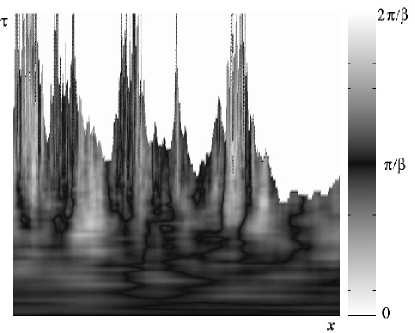
Figure 4: Spacetime structure in a one-dimensional simulation for the two-field model showing the evolution of a comoving region of initial size $l=H^{-1}$ with initially homogeneous $\phi=0$ and $\chi=\pi/\beta$. The values of the field $\chi$ are shown throughout the inflating region using different shades of grey. The shading code is indicated in the bar on the right of the figure. The thermalized regions are left white.

Note that the thermalized regions in Fig.4 have a fractal-like pattern, with larger numbers of increasingly narrow “spikes” appearing at later times. These spikes represent newly-formed thermalized regions, and although they are rather small, their number grows exponentially with time, and they actually dominate the thermalized volume. A change of the time variable $t$ results in a deformation of the cutoff surface, accompanied by a (substantial) change in the population of the newly-formed regions that are being included. This is the origin of the gauge dependence of the cutoff procedure.

4 The proposal

The resolution of the gauge dependence problem that I proposed in Ref.[16] is to calculate the probability distribution for $\chi$ within a single, connected thermalized domain. Each thermalized domain can be infinitely extended and contains an infinite number of galaxies, but it is sufficient to use a large finite part of the domain. If the field $\chi$ varies in a finite range, it will run through all of its values many times in a sufficiently large volume. We expect, therefore, that the distribution $F(\chi)$ will converge rapidly as the volume is increased. It does not matter which thermalized domain we choose to calculate probabilities: all domains are statistically equivalent, due to the stochastic nature of quantum fluctuations in eternal inflation. This is a very simple prescription, and I am a bit embarrassed that I did not think of it earlier, having thought about this problem for a number of years.

With this prescription, the volume distribution $F(\chi)$ can be calculated directly from numerical simulations, and we have done that in [13] for the two-field model (16). In some cases an analytic calculation is also possible. Suppose, for example, that the potential $V(\varphi,\chi)$ is essentially independent of $\chi$ for $|\varphi|<\varphi_{0}$, where $\varphi_{0}$ is in the deterministic slow-roll range, where quantum fluctuations of $\phi$ and $\chi$ can be neglected compared to the classical drift. (The corresponding conditions on the parameters of the potential (16) are specified in [16, 13]). Then, the evolution of $\varphi$ at $\varphi>\varphi_{0}$ is monotonic, and a natural choice of the time variable in this range is $t=\varphi$. The probability distribution for $\chi$ on the constant-”time” surface $\varphi=\varphi_{0}$ is

$$F_{0}(\chi)=F(\varphi_{0},\chi)=const,$$ (17)

since all values of $\chi$ are equally probable at $\varphi<\varphi_{0}$. We are interested in the probability distribution on the thermalization surface, $F(\chi)=F(\varphi_{*},\chi)$, where $\varphi_{*}$ is the value of $\varphi$ at thermalization. This is given by [16]

$$F(\chi)\propto F_{0}(\chi_{0})\exp[3N(\chi_{0})]det\left|{{\partial\chi_{0}}\over{\partial\chi}}\right|.$$ (18)

Here, $\chi_{0}$ is the value of $\chi$ at $\varphi=\varphi_{0}$ that classically evolves into $\chi$ at $\varphi_{*}$, $N(\chi_{0})$ is the number of e-foldings along this classical path, $\exp(3N)$ is the corresponding enhancement of the volume, and the last factor is the Jacobian transforming from $\chi_{0}$ to $\chi$. In many interesting cases, $\chi$ does not change much during the slow roll. Then,

$$F(\chi)\propto\exp[3N(\chi)].$$ (19)

In a more general case, when the diffusion of $\chi$ is not negligible at $\varphi>\varphi_{0}$, the distribution $F(\chi)$ can be found by solving the Fokker-Planck equation with $t=\varphi$ in the range $\varphi_{0}<\varphi<\varphi_{*}$ and with the initial condition (17). The corresponding form of the equation was derived in [13],

$${\partial F\over{\partial\varphi}}=-\partial_{\chi}^{2}\left({H^{3}F\over{2\pi{H^{\prime}}_{\varphi}}}\right)-\partial_{\chi}\left({{H^{\prime}}_{\chi}\over{{H^{\prime}}_{\varphi}}}F\right)-{12\pi H\over{{H^{\prime}}_{\varphi}}}F.$$ (20)

We have solved this equation for the two-field model (16) with the same parameters that we used in numerical simulations and compared the resulting probability distribution $F(\chi)$ with the distribution obtained directly from the simulations. We found very good agreement between the two (see Ref.[13] for details).

5 Density fluctuations

As a specific application of the proposed approach, let us consider the spectrum of density perturbations in the standard model of inflation with a single field $\varphi$. The perturbations are determined by quantum fluctuations $\delta\varphi$; they are introduced on each comoving scale at the time when that scale crosses the horizon and have a gauge-invariant amplitude [7]

$$\delta\rho/\rho=8\pi H\delta\varphi/H^{\prime},$$ (21)

where $H^{\prime}=dH/d\varphi$. With an rms fluctuation $(\delta\varphi)_{rms}=H/2\pi$, this gives

$$(\delta\rho/\rho)_{rms}=4H^{2}/|H^{\prime}|.$$ (22)

Fluctuations of $\varphi$ on different length scales are statistically independent and can be treated separately. We can therefore concentrate on a single scale corresponding to some value $\varphi=\varphi_{0}$, disregarding all of the rest.

On the equal-”time” surface $\varphi=\varphi_{0}$, the fluctuations $\delta\varphi$ can be regarded as random Gaussian variables with a distribution

$$F_{0}(\delta\varphi)\propto\exp\left[-{2\pi^{2}\over{H_{0}^{2}}}(\delta\varphi)^{2}\right],$$ (23)

where $H_{0}=H(\varphi_{0})$. We are interested in the distribution $F(\delta\varphi)$ on the thermalization surface $\varphi=\varphi_{*}$. This will be different from $F_{0}$ if there is some correlation between $\delta\varphi$ and the amount of inflationary expansion in the period between $\varphi_{0}$ and $\varphi_{*}$. In fact, there is such a correlation. If $\varphi$ fluctuates in the direction opposite to the classical roll, then inflation is prolonged and the expansion factor is increased. Otherwise, it is decreased, and we can write

$$F(\delta\varphi)\propto F_{0}(\delta\varphi)\exp(3H_{0}\delta t),$$ (24)

where

$$\delta t=-(4\pi/{H^{\prime}}_{0})\delta\varphi$$ (25)

is the time delay of the slow roll due to the fluctuation $\delta\varphi$.

Combining Eqs.(23)-(25), we obtain [16]

$$F(\delta\varphi)\propto\exp\left[-{2\pi^{2}\over{H_{0}^{2}}}(\delta\varphi-{\bar{\delta\varphi}})^{2}\right],$$ (26)

which describes Gaussian fluctuations with a nonzero mean value,

$${\bar{\delta\varphi}}=3H_{0}^{3}/\pi{H^{\prime}}_{0}.$$ (27)

This is different from the standard approach [7] which disregards the volume enhancement factor and uses the distribution (23). The effect, however, is hopelessly small. Indeed,

$${{\bar{\delta\varphi}}\over{(\delta\varphi)_{rms}}}={6H_{0}^{2}\over{{H^{\prime}}_{0}}}\sim\left({\delta\rho\over{\rho}}\right)_{rms}\sim 10^{-5}.$$ (28)

We thus see that the standard results remain essentially unchanged.

6 Conclusions

Eternally inflating universes can contain thermalized regions with different values of the cosmological parameters, which we have denoted generically by $\chi$. We cannot then predict $\chi$ with certainty and can only find the probability distribution ${\cal P}(\chi)$. Until recently, it was thought that calculation of ${\cal P}$ inevitably involves comparing infinite volumes, and therefore leads to ambiguities. My proposal is to calculate ${\cal P}$ in a single thermalized domain. The choice of the domain is unimportant, since all thermalized domains are statistically equivalent. This apprach gives unambiguous results. When applied to the spectrum of density fluctuations, it recovers the standard results with a small correction $O(10^{-5})$.

It should be noted that this approach cannot be applied to models where $\chi$ is a discrete variable which takes different values in different thermalized regions, but is homogeneous within each region. [An example of such a model is the one-field model (15).] One can take this as indicating that no probability distribution for a discrete variable can be meaningfully defined in an eternally inflating universe. Alternatively, one could try to introduce some other cutoff prescription to be applied specifically in the case of a discrete variable. Some possibilities have been discussed in [17, 18]. This issue requires further investigation.

References

- [1] A. Vilenkin, Phys. Rev. D27, 2848 (1983).
- [2] A. D. Linde, Phys. Lett. B175, 395 (1986).
- [3] A. Vilenkin, Phys. Rev. Lett. 74, 846 (1995).
- [4] A. D. Linde, D. A. Linde, and A. Mezhlumian, Phys. Rev. D49, 1783 (1994).
- [5] S. Winitzki and A. Vilenkin, Phys. Rev. D53, 4298 (1996).
- [6] A. D. Linde, D. A. Linde, and A. Mezhlumian, Phys. Lett. B345, 203 (1995); Phys. Rev. D54, 2504 (1996).
- [7] For a review of density fluctuations in inflationary scenarios, see, e. g., V. F. Mukhanov, H. A. Feldman, and R. H. Brandenberger, Phys. Rep. 215, 203 (1992).
- [8] A. A. Starobinsky, in Lecture Notes in Physics Vol. 246 (Springer, Heidelberg, 1986).
- [9] A.S. Goncharov, A.D. Linde and V.F. Mukhanov, Int. J. Mod. Phys. A2, 561 (1987).
- [10] Y. Nambu and M. Sasaki, Phys. Lett. B219, 240 (1989); K. Nakao, Y. Nambu and M. Sasaki, Prog. theor. phys. 80, 1041 (1988).
- [11] D. S. Salopek and J. R. Bond, Phys. Rev.D43, 1005 (1991).
- [12] M. Aryal and A. Vilenkin, Phys. Lett. B199, 351 (1987).
- [13] V. Vanchurin, A. Vilenkin and S. Winitzki, gr-qc/9905097.
- [14] S. Winitzki and A. Vilenkin, gr-qc/9911029.
- [15] A.D. Linde, Phys. Lett. B 327, 208 (1994); A. Vilenkin, Phys. Rev. Lett. 72, 3137 (1994).
- [16] A. Vilenkin, Phys. Rev. Lett. 81, 5501 (1998).
- [17] A. Vilenkin, Phys. Rev. D52, 3365 (1995).
- [18] A. Vilenkin and S. Winitzki, Phys. Rev. D55, 548 (1997).