Toward gravitational wave detection

Abstract

An overview of some tools and techniques being developed for data conditioning (regression of instrumental and environmental artifacts from the data channel), detector design evaluation (modeling the science “reach” of alternative detector designs and configurations), noise simulations for mock data challenges and analysis system validation, and analyses for the detection of gravitational radiation from gamma-ray burst sources.

I Detector Characterization

Quality data analysis requires quality data. Part of the process of producing quality data is identifying and, as far as possible, removing instrumental and environmental artifacts. Here we illustrate, using data taken during November 1994 at the LIGO 40 M prototype, the identification and removal, through linear regression, of artifacts due to harmonics of the 60Hz power mains.

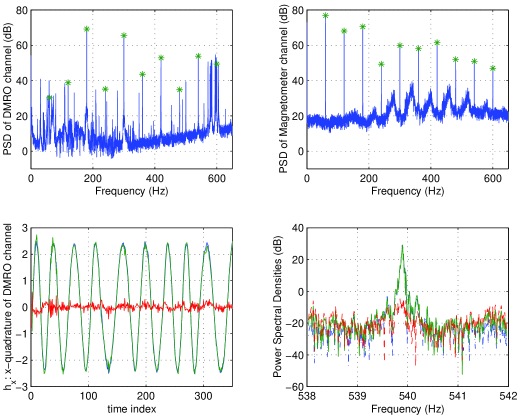
A power spectrum (psd) of the LIGO 40 M IFO_DMRO (interferometer differential-mode read-out; hereafter, “gravity-wave”) channel shows a series of narrow spectral features at 60 Hz and its harmonics. Similar narrow spectral features are evident in the magnetometer channel, IFO_MAGX, which was recorded simultaneously with the gravity wave channel.

Focus attention, in both the magnetometer and gravity-wave channel, on a narrow band about one of the harmonics. We suppose that, in this narrow band, the gravity wave channel $h$ is related to the magnetometer channel $M$ through an expression of the form

$$h[k]={B(q)\over A(q)}M[k-n]+{C(q)\over D(q)}e[k],$$ (1)

where the index $k$ indicates the sample number, the residual $e[k]$ is white and $A(q),B(q),C(q)$ and $D(q)$ are polynomials in the lag operator $q^{-1}$,

$$q^{-1}M[k]:=M[k-1].$$ (2)

The ratio $B(q)/A(q)$ is a linear filter that can be thought of as the transfer function between the magnetometer and the gravity wave channel; similarly, the ratio $D(q)/C(q)$ can be thought as a filter that whitens that part of the gravity wave channel not explained by the magnetometer channel.

Using a small sample of data we find the “best” filters $B(q)/A(q)$ and $C(q)/D(q)$, where better choices yield smaller residuals and have fewer poles and zeros. (Fewer poles and zeros are desired because we don’t want to over fit the data; smaller residuals are desired because we want to identify everything in $h$ that can be explained by $M$.)

To illustrate, we focus on the 540 Hz harmonic in an approximately 2666 second continuous stretch of LIGO 40 M data taken on 19 November 1994. We mix this harmonic down to zero frequency and down-sample the data to a 4 Hz bandwidth. Using a $100$ second segment of data from both the magnetometer and gravity wave channels, we find the filters $B(q)/A(q)$ and $C(q)/D(q)$ and the lag $n$. In this case the best filters have six zeros and one pole each. The quantity

$$h[k]-{B(q)\over A(q)}M[k-n]$$ (3)

is then as free from the effects of the 540 Hz harmonic as we can make it, under the hypotheses of this model.

Figure 1: 60 Hz harmonics and their regression from the interferometer data stream. See section I for details.

Figure 1 shows the effectiveness of this analysis. The top two panels show the gravity wave and magnetometer channel psd, with the 60 Hz harmonic features marked with asterisks. In the left bottom panel one curve shows one quadrature of the mixed and decimated gravity wave channel, a second shows the prediction that comes from applying the filter $B(q)/A(q)$ to the lagged magnetometer channel, and the third is their difference (cf. eq. 3). The final panel shows the psd of this difference, superposed with the psd of the original $h[k]$ and the magnetometer prediction. The magnetometer channel explains 40 dB of the contamination of the gravity wave channel by the 540 Hz harmonic.

II Benchmarks for detector design

Gravitational wave detectors are built to detect gravitational waves. Better detectors do a better job of detecting gravitational waves. But, what are the relative advantages of, e.g., better sensitivity in a narrow band as opposed to somewhat worse sensitivity, but over a broader band? How do we quantify better? To aid in answering this question we have developed a Matlab model, bench, that calculates different figures of merit, based on source science, for use in detector design and configuration trade studies.

An interferometer is described to bench in terms its laser, optical surface, suspension and substrate properties, since it is these that determine the dominant contributions to the detectors noise performance. From this characterization bench determines the detectors expected thermal noise in the mirror suspensions and substrates, radiation pressure and laser shot noise. Using this idealized noise model bench calculates two different figures of merit: the first, an effective distance to which inspiraling binary neutron stars can be observed above a fixed threshold signal-to-noise, and the second, a measure of the upper-bound that can be placed on the intensity of a stochastic gravitational-wave background in the LIGO detector system, assuming identical interferometers installed at each observatory.

The bench model for the principal interferometer noise sources has the following features:

• Radiation pressure and laser shot noise expressions support interferometer configurations including power recycling and resonant sideband extraction through the specification of three mirror transmittances and associated losses in the optical system. Thermal lensing effects are estimated and a warning issued if the laser power on the beam splitter exceeds the bounds permitted by the losses in the optical system.

• The suspension thermal noise model includes thermoelastic and structural damping for ribbon and cylindrical suspensions composed of different materials (and, for ribbon suspensions, different aspect ratios) rowan97a ; rowan97b ;

• Thermal noise in the (cylindrical) mirror substrates depends on substrate dimensions, material properties (Young modulus, Poisson ratio, loss angle), and the incident (laser) beam radius bondu98a .

The binary inspiral “effective distance” figure of merit is a distance $r_{0}$ such that the observed rate of inspiraling binary neutron star systems with S/N greater than 8 is equal to $4\pi r_{0}^{3}\dot{n}/3$, where $\dot{n}$ is the rate per unit volume of inspiraling binary systems finn96a . The stochastic signal sensitivity benchmark determines a threshold on the cross-correlation between two identical detectors (located and oriented like the LIGO detectors) such that, in the absence of a stochastic signal (or any other cross-correlated noise), the cross-correlation estimated using 1/3 yr data would exceed this threshold in only one of every one hundred trials. Other benchmarks are planned.

Figure 2: A noise model produced by bench, a tool for use in evaluating the science reach of different interferometric detector configurations or designs. An interferometer with this configuration can observe binary inspiral in an effective volume of radius 288 Mpc. See section II for details.

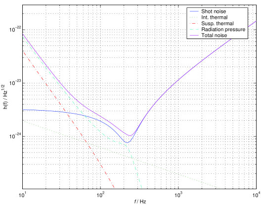
Figure 2 shows a sample noise model produced by bench for an interferometer whose parameters are those described in gustafson99a as a possible LIGO II goal, but whose mirror reflectivities are optimized to maximize the distance to which neutron star binary inspirals could be observed. In this configuration, a single interferometer could survey an effective volume of radius 290 Mpc for neutron star binary inspirals: a volume large enough to expect an event rate of just less than one per month. The two LIGO interferometers operating in this configuration would observe an effective volume $2^{1/2}$ times large, with an expected event rate of one just less than once every two weeks.

III Mock data for mock data challenges

Reliable analysis software is a prerequisite for reliable data analysis. Validating the performance of analysis system software will involve “Mock-Data Challenges” (MDCs). In a MDC, “mock data” — artificially generated time-series whose statistical character and signal content is known exactly — is passed through an analysis pipeline.

MDCs take two forms. In the first, idealizations of the detector noise, for which the pipeline response can be anticipated, are constructed and passed through the analysis pipeline. Agreement between the anticipated and actual system response validates the analysis system implementation. In the second form, more faithful simulations of detector noise are used to calibrate the analysis system: i.e., determine, in a realistic but controlled environment, the detection efficiency and false alarm frequency as a function of the pipeline thresholds associated with the selections and data cuts.

In either form, mock data always includes the fundamental noise sources that contribute the greatest part of the detector noise power. In existing and planned interferometric detectors these fundamental contributions arise from radiation pressure noise, laser shot noise, suspension and substrate thermal noise. The thermal noise contributions have the character of structurally damped harmonic oscillators with small loss angles. The significant contribution from the substrate thermal noise arises from the low-frequency tail of the noise distribution, whose power spectral density (psd) is proportion to $f^{-1}$. The significant contribution from the suspension thermal noise arises from the high-frequency tail of the suspension pendulum mode, where the psd is proportional to $f^{-5}$. Additionally, the resonant peaks associated with the weakly damped suspension violin modes contribute important instrumental artifacts that must be part of a realistic noise simulation.

The general plan of our noise simulator is to find a combination of linear filters, acting in parallel on independent white noise sequences, whose sum gives rise to a sequence whose power spectral density (psd) has the desired form. The design of short, effective linear filters that capture either the odd-power dependence on $f$ characteristic of the thermal noise tail of structurally damped oscillators, or the strong resonant peaks of the weakly damped systems, has been a stumbling block in this program. We have overcome those difficulties by developing a physical model of a structurally damped system whose noise psd has the desired in-band character. Arising from a physical model, the psd can be factored into a real, linear, zero-pole-gain filter that is stable and invertible (i.e., has all of its poles in the left half-plane and zeros in the right half-plane), and with the required magnitude response. The filter’s zeros, poles and gain are determined uniquely and directly by location and quality factor of the resonance, and the desired simulation bandwidth.

Figure 3: Simulations of the principle contributions to the overall noise of an interferometric gravitational wave detector. For more details see section III.

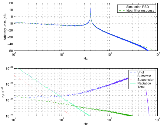
The first panel of figure 3 shows the psd of noise simulated to have the character of a structurally damped harmonic oscillator over three decades in frequency above and below the resonance. The simulation psd is overlaid with the spectrum of an idealized structurally damped harmonic oscillator with the same loss-angle and resonance frequency. This model involved thirteen poles and an equal number of zeros. They agree to better than 1% over the detector bandwidth. The second panel shows the noise psd of the other components of the simulation (radiation pressure, shot, internal thermal and pendulum mode suspension thermal noise) for a LIGO II like interferometer without resonant sideband extraction.

IV Gravitational waves and $\gamma$-ray bursts

Gamma-ray bursts (GRBs) are likely triggered by the violent formation of a solar mass black hole, surrounded by a debris torus, at cosmological distances. Given the distance, the violence of the formation event, and the range of possible progenitors, waveforms from events like these cannot be predicted a priori, nor the gravitational radiation associated with an individual burst detected directly.

Nevertheless, if GRBs are accompanied by gravitational wave bursts (GWBs) the correlated output of two gravitational wave detectors evaluated in the moments just prior to a GRB will differ from that evaluated at other times. This difference can be detected, with increasing sensitivity as the number of detector observations coincident with GRBs increases. Observations at the two LIGO observatories, operating at the anticipated LIGO I sensitivity and coincident with 1000 GRBs, can be used to set a 95% confidence upper limit of ${h}_{\text{RMS}}\sim 1.7\times 10^{-22}$ on the gravitational waves associated with GRBs. (See finn99f for more details.)

Consider the correlation $X$ between the output $h_{1}$ and $h_{2}$ of two LIGO gravitational wave detectors:

$$X := \langle x_{1},x_{2}\rangle=\int\int_{0}^{T}dt\,dt^{\prime}\,x_{1}(t)Q(|t-t^{\prime}|)x_{2}(t^{\prime}),$$ (4)

where we have adjusted the origin of time in each detector so that plane gravitational waves from a direction $\vec{n}$ arrive “simultaneously” in the two detectors. Assuming that GWB signals from GRBs are broadband bursts, take the Fourier transform of $Q$ to be $\widetilde{Q}(f)=\left(S_{1}(|f|)S_{2}(|f|)\right)^{-1}$, where $S_{i}(f)$ is the power spectral density (psd) of detector $i$, for $f$ in the detector band, and $0$ otherwise.

Every time a GRB occurs (say, at time $t_{0}$) adjust the origin of time so that $\vec{n}$ points towards the GRB and form $X$ with the interval $(t_{0}-T,t_{0})$ of data from the two detectors. The duration $T$ of this interval we choose large enough so that we are likely to have included in the interval any associated GWB. For current models of gamma-ray bursts this is no longer than several hundred seconds (where we have accounted for the cosmological redshift of these distant sources).

For each observed GRB we thus have an $X$. Collect these $X$ into the on-source observation set ${\cal X}_{\rm{on}}$. Similarly, we build an off-source observation set ${\cal X}_{\rm{off}}$ following the same procedure but choosing random times $t_{0}$, not associated with any GRBs, and random directions $\vec{n}$ in the sky.

Assuming that GRB signals are weak compared to the detector noise, the sample sets ${\cal X}_{\rm off}$ and ${\cal X}_{\rm on}$ differ only in their means. This difference, $\overline{s}$ is just the average over the source population of $\langle h_{1},h_{2}\rangle$, where $h_{k}$ is the GWB signal in detector $k$. For the two LIGO detectors $h_{1}$ and $h_{2}$ are, to a good approximation, identical and $\overline{s}$ is proportional to the mean-square amplitude of the wave of $h$ over the source population.

We can test for the difference in the means of the two distributions ${\cal X}_{\rm{on}}$ and ${\cal X}_{\rm{off}}$ using Student’s $t$-test snedecor67a , a standard test for difference in means. This provides a simple, yes/no answer to the question of whether GWBs are associated with GRBs.

Alternatively, we can use the value of the $t$-statistic to set an upper bound on $\overline{s}$. To assess the strength of the upper bound, assume that there is no gravitational radiation associated with GRBs. In this case the ensemble mean, median and mode of the $t$ statistic is zero. Assuming that we actually observed $t$ equal to zero we would obtain the 95% upper bound

$${h}_{\text{RMS},95\%}^{2} \leq \left[9.4\times 10^{-22}\right]^{2}\left({T\over 500\,\text{s}}{1000\over N_{\text{on}}}\right)^{1/2}{S_{0}\over\left(3\times 10^{-23}\,\text{Hz}^{-1/2}\right)^{2}}\left({\Delta f\over 100\,\text{Hz}}\right)^{3/2}.$$ (5)

where, for convenience, we have modeled the LIGO I detector noise as approximately constant with power spectral density $S_{0}$ over the bandwidth $\Delta f$, and much higher elsewhere. The value of $T$ adopted here is consistent with external shock models of GRBs; if, on the other hand, it becomes clear that internal shock models are more appropriate (as is becoming more likely), then $T$ will be reduced by a factor of 1000 and the limit will improve by a factor of nearly six.

This upper limit is remarkably strong, especially because it arises without assuming any model for the GWB source or waveform, or the detector noise. Focusing on the difference in the population means has the important consequence that noise correlated between the detectors, but not associated with gravitational waves from GRBs, does not affect the difference in the means. Correspondingly, statistical tests built around the difference in the means are insensitive to noise correlated between the two gravitational wave detectors. Observations with this sensitivity will have important astrophysical consequences, either confirming or constraining the black hole model for GRBs, neither or which can be done with strictly electromagnetic observations.

V Acknowledgments

We are grateful to the LIGO Laboratory for permitting the use of LIGO 40M prototype data in this work. The research described here is funded by United States National Science Foundation awards PHY 98-00111, 99-6213, 98-00970, 96-02157, 96-30172; the University of Glasgow and the United Kingdom funding agency PPARC.

References

- (1) S. Rowan et al., Phys. Lett. A 227, 152 (1997).
- (2) S. Rowan et al., Phys. Lett. A 233, 303 (1997).
- (3) F. Bondu, P. Hello, and J.-Y. Vinet, Phys. Lett. A 246, 227 (1998).
- (4) L. S. Finn, Phys. Rev. D 53, 2878 (1996).
- (5) E. Gustafson, D. Shoemaker, K. Strain, and R. Weiss, Technical Report No. LIGO-T990080, LIGO, LIGO Laboratory, California Institute of Technology (unpublished).
- (6) L. S. Finn, S. D. Mohanty, and J. D. Romano, Detecting an association between Gamma Ray and Gravitational Wave Bursts, 1999, in press, Physical Review D.
- (7) G. W. Snedecor and W. G. Cochran, Statistical Methods (Iowa State University Press, Ames, Iowa, 1967).