MPI–PhT–99/46
LMU–TPW–99/18

This series of lectures presented at the 35th Karpacz Winter School on Theoretical Physics: From Cosmology to Quantum Gravity gives a simple and self-contained introduction to the non-perturbative and background independent loop approach of canonical quantum gravity. The Hilbert space of kinematical quantum states is constructed and a complete basis of spin network states is introduced. An application of the formalism is provided by the spectral analysis of the area operator, which is the quantum analogue of the classical area function. This leads to one of the key results of loop quantum gravity: the derivation of the discreteness of the geometry and the computation of the quanta of area. Finally, an outlock on a possible covariant formulation of the theory is given leading to a “sum over histories” approach, denoted as spin foam model. Throughout the whole lecture great significance is attached to conceptual and interpretational issues. In particular, special emphasis is given to the role played by the diffeomorphism group and the notion of observability in general relativity.

1 Introduction

In the beginning of this century, physics has undergone two great conceptual changes. With the discovery of general relativity and quantum mechanics the notions of matter, causality, space and time experienced the biggest modifications since the age of Descartes, Copernicus, and Newton. However, no fully convincing synthesis of these theories exists so far. Simple dimensional analysis reveals that new predictions of a quantum theory of gravitation are expected to take place at the Planck length $l_{P}\equiv\left(\hbar G/c^{3}\right)^{1/2}\sim 10^{-35}\,\mbox{m}$. This scale appears to be far below any current experimental technique. Nevertheless, quite recently interesting proposals and ideas to probe experimentally the physics at the Planck scale have been suggested [1, 2].

From the theoretical point of view, several approaches to a theory of quantum gravity have emerged, inspired by various research fields in contemporary physics and mathematics. The most popular research direction is string theory, followed by loop quantum gravity. Other directions range from discrete methods to non-commutative geometry. We have listed the main current approaches to a quantum theory of gravity (which are, by the way, far from being independent) in Table 1. Despite this variety of ideas and the effort put in so far, many questions are still open. For an overview and a critical comparison of the different approaches, see [3].

Traditional	Most Popular	New
Discrete methods   Dynamical triangulations   Regge calculus   Simplicial models	String theory  $\rightarrow$ Black hole entropy	Non-commutative geometry
Approximate theories   Euclidean quantum gravity   Perturbative quantum gr.   QFT on curved space–times	Loop quantum gravity   $\rightarrow$ Black hole entropy   $\rightarrow$ Eigenvalues of geometry: $\!A_{\vec{j}}=8\pi\hbar G\sum_{i}\sqrt{j_{i}(j_{i}+1)}$	Null surfaces
		Spin foam models   $\rightarrow$ convergence of loop,       discrete, TQFT       and sum-over-histories
Unorthodox approaches   Sorkin’s Posets   Finkelstein   Twistors   …

Table 1: The main current approaches to quantum gravity.

String theory was inspired and constructed mainly by particle physicists. Its attitude towards the fundamental forces is to treat general relativity on an equal footing with the field theories describing the other interactions, the destinctive feature being the energy scale. String theory is supposed to be a theory of all interactions—electromagnetic, strong, weak and gravitational— which are treated in a unified quantum framework. Classical (super-)gravity emerges perturbatively as a low-energy limit in superstring theory. Until 1995 the problem was the lack of a non-perturbative formulation of the theory. This situation has improved with the discovery of string dualities, “D-branes”, and “M-theory” in the so-called 2nd superstring revolution. Nevertheless, despite the recent exciting discoveries in M-theory and the AdS/CFT equivalence, a complete non-perturbative or strong-coupling formulation of string/M-theory is still not in sight.

A point that is often criticized in string theory by relativists is the lack of a background independent formulation, i.e. invariance under active diffeomorphisms, which is one of the fundamental principles of general relativity. String/M-theory is formulated on a (implicitly) fixed background geometry which is itself not dynamical. In a truely background independent formulation, no reference to any classical metric should enter neither the definition of the state space nor the dynamical variables of the theory. Rather the metric should appear as an operator allowing for quantum states which may themselves be superpositions of different backgrounds.

In fact, relativists do not view general relativity as an additional item in the list of the field theories describing fundamental forces, but rather as a major change in the manner space and time are described in physics. This point is often misunderstood, and is often a source of confusion; it might be worthwhile spending a few additional words. The key point is not that the gravitational force, by itself, must necessarilly be seen as different from the other forces: the point of view that the gravitational force is just one (and the weakest) among the interactions is certainly viable and valuable. Rather, the key point is that, with general relativity, we have understood that the world is not a non-dynamical metric manifold with dynamical fields living over it. Rather, it is a collection of dynamical fields living, so to say, in top of each other. The gravitational field can be seen—if one wishes so—as one among the fields. But the definiton of the theory over a given background is, from a fundamental point of view, physically incorrect.

Loop quantum gravity is a background independent approach to quantum gravity. For many details on this approach, and for complete references, see [6]. Loop quantum gravity has been developed ab initio as a non-perturbative and background independent canonical quantum theory of gravity. Besides ordinary general relativity and quantum mechanics no additional input is needed. The approach makes use of the reformulation of general relativity as a dynamical theory of connections. Due to this choice of variables the phase space of the theory resembles at the kinematical level closely that of conventional $SU(2)$ Yang–Mills theory. The main ingredient of the appraoch is the choice of holonomies of the connections—the loop variables—as the fundamental degrees of freedom of quantum gravity.

The philosophy behind this approch is different from string theory as one considers here standard 4-dimensional general relativity trying to develop a theory of quantum gravity in its proper meaning without claiming to describe a unified picture of all interactions. Loop quantum gravity is successful in describing Planck-scale phenomena. The main open problem, on the other hand, is the connection with low-energy phenomena. In this respect loop quantum gravity has opposite strength and weakness than string theory. However, some of the conceptually different approaches that were given in Table 1 show surprising similarities which could be a focal point of attention for the future .

One might wonder how one can hope to have a consistent non-perturbative formulation of quantum gravity when perturbative quantization of covariant general relativity is non-renormalizable. However, the basic assumption in proving the non-renormalizability of general relativity is the availability of a Minkowskian space–time at arbitrarily short distances, an assumption which is certainly not correct in a theory of quantized gravity, i.e. in a quantum space–time regime. As will be discussed later, one of the key results obtained so far in loop quantum gravity has been the calculation of the quanta of geometry [7], i.e. the spectra of the quantum analogues to the classical area and volume functionals. Remarkably they turned out to be discrete! This result (among similar ones obtained in other approaches, see footnote 1) indicates the existence of a quantum space–time structure at the Planck scale which doesn’t have to be continuous anymore. More specifically this implies the emergence of a natural cut-off in quantum gravity that might also account as a regulator of the ultraviolet divergencies plaguing the standard model. Thus, standard perturbative techniques in field theory cannot be taken for granted at scales where quantum effects of gravity are expected to dominate.

General relativity is a constrained theory. Classically, the constraints are equivalent to the dynamical equations of motion. The transition to the quantum theory is carried out using canonical quantization by appliying the algorithm developed by Dirac [8]. In the loop approach, the unconstrained classical theory is quantized, requiring the implementation of quantum constraint operators afterwards. Despite many results obtained in the last few years, a complete implementation of all constraints including the Hamiltonian constraint, which is the generator of “time evolution”, i.e. the dynamical part of the theory, is still elusive. This is of course not surprising, since we do not expect to be able to obtain a complete solution of a highly non-trivial and non-linear theory. To address this issue, covariant methods to understand the dynamics have been developed in the last few years. These can be obtained from a “sum over histories” approach, derived from the canonical formulation. This development has led to the so-called spin foam models, in which spin networks are loosely speaking “propagated in time”, leading to a space–time formulation of loop quantum gravity. This formulation of the theory provides a starting point for approximations, offers a more intuitive understanding of quantum space–time, and is much closer to particle physics methods. A brief description will be given below in sect. 5.2.

These lectures are organized as follows. We start in sect. 2 with the basic mathematical framework of loop quantum gravity and end up with the definition of the kinematical Hilbert space of quantum gravity. In the next section an application of these tools is provided by constructing the basic operators on this Hilbert space. We calculate in a simple manner the spectrum of what is going to be physically interpreted as the area operator. Section 4 deals with the important question of observability in classical and quantum gravity, a topic which is far from being trivial, and the meaning of diffeomorphism invariance in this context. In the end of theses notes, we will give the prospects for a dynamical description of loop quantum gravity, which is encoded in the concept of spin foam models. One such ansatz is briefly discussed in sect. 5. The following final section concludes with future perspectives and open problems.

For the sake of completeness, we give in Table 2 a short historical survey of the main achievements in canonical quantum gravity since the reformulation of general relativity in terms of connection variables. A more detailled discussion of some of these aspects and full bibliography is given in [6].

’86	Classical Connection Variables	[9, 22, 23]
’87	Lattice Loop States solve $\hat{H}$	[10]
’88	Loop Quantum Gravity	[27, 28]
’92	Weave States	[11]
’92	Diffeomorphism Invariant Measure	[12, 13]
’95	Spin Network States	[30]
’95	Volume and Area Operators	[7]
’95	Functional Calculus	[14, 15]
’96	Hamiltonian Operator	[24, 25]
’96	Black Hole Entropy	[16, 17, 18]
’98	Spin Foam Formulation	[46, 47]

Table 2: A short historical survey of canonical quantum gravity, with some relevant references.

2 The Basic Formalism of Loop Quantum Gravity

Our attention in this lecture will be focused on conceptual foundations and the development of the main ideas behind loop quantum gravity. However, because of the highly mathematical nature of the subject some technical details are unavoidable, thus this section is devoted to the essential mathematical foundations.

The reader is not assumed to be familiar with the connection variables, which constitute the basis for most efforts in canonical quantum gravity since 1986. Thus we start by considering the canonical formalism in the connection approach, which is reviewed in [19]. For a recent overview of loop quantum gravity and a comprehensive list of references we refer to [6].

2.1 A brief Outline of the Connection Formalism

In loop quantum gravity, we construct the quantum theory using canonical quantization. This is analogous to ordinary field theory in the functional Schrödinger representation. The approach may be called conservative in the sense that originally no new structures like supersymmetry, extended objects, or extra dimensions are postulated. (It is important to emphasize, in this context, the fact, sometimes forgotten these days, that supersymmetry, extended objects or extra dimensions are interesting theoretical hypotheses, not established properties of Nature!). The approach aims at unifying quantum mechanics and general relativity by developing new non-perturbative techniques from the outset and by staying as close as possible to the conventional settings of quantum theory and experimentally tested general relativity.

The foundations of the formalism date back to the early 60s when the “old” Hamiltonian or canonical formulation of classical general relativity, known as ADM formalism, was constructed. The canonical scheme is based on the construction of the phase space $\Gamma$. Phase space is a covariant notion. It is the space of solution of the equations of motion, modulo gauges. However, in order to coordinatize $\Gamma$ explicitly, one usually breakes explicitly covariance and splits 4-dimensional space–time $\mathcal{M}$ into 3-dimensional space plus time. We insist on the fact that this breaking of covariance is not structurally needed in order to set up the canonical formalism; rather it is an artefact of the coordinatization we choose for the phase space. We take $\mathcal{M}$ to have topology $\mathbb{R}\times M$, and we cover it with a foliation $M_{t}$. Here $M$ is the 3-manifold representing “space” and $t\in\mathbb{R}$ is a (unphysical) time parameter. The basic variables on phase space are taken to be the induced 3-metric $q_{ab}(x)$ on $M$ and the extrinsic curvature $K_{ab}$ of $M$.

The easiest construction of the connection variables is given by first reformulating the ADM–formalism of canonical gravity in terms of (local) triads $e^{i}_{a}(x)$, which satisfy $q_{ab}(x)=e^{i}_{a}(x)e^{i}_{b}(x)$. This introduces an additional local $SU(2)$ gauge symmetry into the theory, which geometrically corresponds to arbitrary local frame rotations. One obtains $\big{(}E^{a}_{i}(x),K^{i}_{a}(x)\big{)}$ as the new canonical pair on phase space $\Gamma$. $E^{a}_{i}$ is the inverse densitized triad, i.e. a vector with respect to $SU(2)$ and density weight one. The densitized triad itself is defined by $E^{i}_{a}:=e\,e^{i}_{a}$, where $e$ is the determinant of $e^{i}_{a}$. The indices $a,b,\ldots=1,2,3$ refer to spatial tangent space components, while $i,j,\ldots=1,2,3$ are internal indices that can be viewed as labelling either the axis of a local triad or the basis of the Lie algebra of $SU(2)$. The inverse triad $E^{a}_{i}$ is the square-root of the 3-metric in the sense that

$$E^{a}_{i}(x)E^{b}_{i}(x)=q(x)\,q^{ab}(x)\;,$$ (1)

where $q(x)$ is the determinant of the 3-metric $q_{ab}(x)$. The canonically conjugate variable $K^{i}_{a}(x)$ of $E^{a}_{i}(x)$ is again closely related to the extrinsic curvature of $M$ via $K^{i}_{a}=K_{ab}E^{bi}\!/\!\sqrt{q}$.

The transition to the connection variables is made using a canonical transformation on the (real) phase space,

$$A^{i}_{a}(x)=\Gamma^{i}_{a}(x)+\beta\,K^{i}_{a}(x)\;.$$ (2)

Here $\Gamma^{i}_{a}(x)$ is the $SU(2)$ spin connection compatible with the triad, and $\beta$, the Immirzi parameter, is an arbitrary real constant. The original Ashtekar–Sen connection $A(x)$ was introduced in 1982 as a complex self-dual connection on the spatial 3-manifold $M$, corresponding to $\beta=i$ in (2). Here we will use the real formulation.

Nevertheless $\big{(}A^{i}_{a}(x),\,E^{a}_{i}(x)\big{)}\in\Gamma$ form a canonical pair on the phase space $\Gamma$ of general relativity [22, 23]. Here $A^{i}_{a}$ has to be considered as the new configuration variable, while the inverse densitized triad $E^{a}_{i}$ corresponds to the canonically conjugate momentum. With this reformulation classical general relativity has the same kinematical phase space structure as an $SU(2)$ Yang–Mills theory.

The Poisson algebra generated by the new variables is

$$\big{\{}E^{a}_{i}(x),\,E^{b}_{j}(y)\big{\}} = 0\;,\hskip 14.22636pt\big{\{}A^{i}_{a}(x),\,A^{j}_{b}(y)\big{\}}=0\;,$$

$$\big{\{}A^{i}_{a}(x),\,E^{b}_{j}(y)\big{\}} = \beta\,G\,\delta^{i}_{j}\,\delta^{b}_{a}\,\delta^{3}(x,y)\;,$$ (3)

where $G$ is the usual gravitational constant. It arises because the conjugate momentum of the configuration variable $A^{i}_{a}$ (obtained as the derivative of the Lagrangian with respect to the velocities) is actually given by $1/G\times E^{a}_{i}$. As a consequence of the 4-dimensional diffeomorphism invariance of general relativity, the (canonical) Hamiltonian vanishes weakly. The full dynamics of the theory is encoded in so-called first-class constraints which are functions on phase space that vanish for physical configurations. The constraints generate transformations between those classical configurations that are physically indistinguishable. The first-class constraints of canonical general relativity are the familiar Gauss law of Yang–Mills theory, which generates local $SU(2)$ gauge transformations, the diffeomorphism constraint generating 3-dimensional diffeomorphisms of the 3-manifold $M$, and the Hamiltonian constraint, which is the generator of the evolution of the inital spatial slice $M$ in coordinate time. The Gauss constraint enters the theory as a result of the choice of triads and it makes general relativity resemble a Yang–Mills gauge theory. And indeed, the phase spaces of both theories are similar. The constrained surface of general relativity is embedded in that of Yang–Mills theory apart from the additional local restrictions which appear in gravity besides the Gauss law.

The use of the set of canonical variables involving a complex connection $A(x)$ leads to a simplification of the Hamiltonian constraint. With the use of a real connection, the constraint loses its simple polynomial form. At first, this was considered as a serious obstacle for quantization. However, Thiemann succeeded in constructing a Lorentzian quantum Hamiltonian constraint [25] in spite of the non-polynomiality of the classical expression. His work has prompted the wide use of the real connection, a use which was first advocated by Barbero [26].

We will now briefly describe the quantum implementation of this kinematical setting. The canonical variables $A$ and $E$ (or functions of these), are replaced by quantum operators acting on a Hilbert space of states, promoting Poisson brackets to commutators. In other words, an algebra of observables should act on a Hilbert space. More precisely, we establishe an isomorphism between the Poisson algebra of classical variables and the algebra generated by the corresponding Hermitian operators by introducing a linear operator representation of this Poisson algebra. The quantum states are normalizable functionals over configuration space, i.e. functionals of the connection $\Psi(A)$ (or limits of these). The subset of physical states is obtained from the set of all wavefunctions on $M$ by imposing the quantum analogues of the contraints, i.e. by requiring the physical states to lie in the kernel of all quantum constraint operators.

The space of physical states must have the structure of a Hilbert space, namely a scalar product, in order to be able to compute expectation values. This Hilbert structure is determined by the requirement that real physical observables correspond to self-adjoint operators. In order to define a Hilbert structure on the space of physical states, it is convenient (althought not strictly necessary) to define first a Hilbert structure on the space of unconstrained states. This is because we have a much better knowledge of the unconstrained observables than of the physical ones. If we choose a scalar product on the unconstrained state space which is gauge invariant, then there exist standard techniques to “bring it down” to the space of the physical states. Thus, we need a gauge and diffeomorphism invariant scalar product, with respect to which real observables are self-adjoint operators.

2.2 Basic Definitions

In this subsection we start with the actual topic of the lecture, the construction of loop quantum gravity. Space–time is assumed to be a 4-dimensional Lorentzian manifold $\mathcal{M}$ with topology $\mathbb{R}\times M$, where $M$ is a real analytic and orientable 3-manifold. For simplicity we take $M$ to be topologically $S^{3}$. Loosely speaking $M$ represents “space” while $\mathbb{R}$ refers to “time”.

On $M$ we define a smooth, Lie algebra valued connection 1-form $A$, i.e. $A(x)=A^{i}_{a}(x)\,\tau_{i}\,dx^{a}$, where $x$ are local coordinates on $M$, $A^{i}_{a}(x)\in C^{\infty}(M)$, and $\tau_{i}=(i/2)\,\sigma_{i}$ are the $SU(2)$ generators in the fundamental representation, satisfying $[\tau_{i},\tau_{j}]=\epsilon_{ijk}\tau^{k}$. Here $\sigma_{i}$ are the Pauli matrices. The indices $a,b,c=1,2,3$ play the role of tangent space indices while $i,j,k=1,2,3$ are abstract internal $su(2):=Lie\big{(}SU(2)\big{)}$ indices. We call $\mathcal{A}=\{A\}$ the space of smooth connections on $M$ and denote continuous functionals on $\mathcal{A}$ as $\Psi(A)$. These functionals build up a topological vector space $L$ under the pointwise topology.

2.3 The Construction of a Hilbert Space $\mathcal{H}$

In order to define a Hilbert space $\mathcal{H}$ based on the above linear space $L$ of quantum states $\Psi(A)$, an inner product needs to be introduced, i.e. an appropriate measure on the space of quantum states is required. For that purpose the appearance of the compact gauge group $SU(2)$ turns out to be essential. We demand the following properties of $\mathcal{H}$:

• $\mathcal{H}$ should carry a unitary representation of $SU(2)$

• $\mathcal{H}$ should carry a unitary representation of $Diff(M)$ .

We construct the inner product by means of a special class of functions of the connection in $L$, the cylindrical functions. For their construction we need some tools, namely holonomies and graphs.

2.3.1 Holonomies.

Let a curve $\gamma$ be defined as a continuous, piecewise smooth map from the intervall $[0,1]$ into the 3-manifold $M$,

$$\gamma:[0,1] \longrightarrow M$$ (4)

$$s \longmapsto \{\gamma^{a}(s)\}\;,\;a=1,2,3\;.$$ (5)

The holonomy or parallel propagator $U[A,\gamma]$, respectively, of the connection $A$ along the curve $\gamma$ is defined by

$$U[A,\gamma](s) \in SU(2)\;,$$ (6)

$$U[A,\gamma](0) = \textup{\small{1}}\kern-3.6pt\textup{1}\ \;,$$ (7)

$$\frac{d}{ds}\,U[A,\gamma](s) + A_{a}\big{(}\gamma(s)\big{)}\,\dot{\gamma}^{a}(s)\,U[A,\gamma](s)=0\;,$$ (8)

where $\dot{\gamma}(s):=\frac{d\gamma(s)}{ds}$ is the tangent to the curve. The formal solution of (8) is given by

$$U[A,\gamma](s)=\mathcal{P}\exp\int_{\gamma}ds\,\dot{\gamma}^{a}\,A_{a}^{i}\big{(}\gamma(s)\big{)}\,\tau_{i}\equiv\mathcal{P}\exp\int_{\gamma}A\;,$$ (9)

in such a way that for any matrix-valued function $A\big{(}\gamma(s)\big{)}$ which is defined along $\gamma$, the path ordered expression (9) is given in terms of the power series expansion

$$\mathcal{P}\exp\int_{0}^{1}ds\,A\big{(}\gamma(s)\big{)}$$ (10)

$$=\sum_{n=0}^{\infty}\,\int_{0}^{1}ds_{1}\int_{0}^{s_{1}}ds_{2}\,\cdots\int_{0}^{s_{n-1}}ds_{n}\,A\big{(}\gamma(s_{n})\big{)}\cdots A\big{(}\gamma(s_{1})\big{)}\;.$$

Here $\mathcal{P}$ denotes path ordering, i.e. the parameters $s_{i}$ are ordered with respect to their moduli from the left to the right, or more explicitely $s_{1}\leq s_{2}\leq\ldots$ .

In a later section we will focus our attention to Wilson loops, which are traces of the holonomy of $A$ along a curve $\gamma$, satisfiying $\gamma(0)=\gamma(1)$, i.e. a closed curve or loop, respectively, which in the following will be denoted as $\alpha$. We write

$$T[A,\alpha]=-\mbox{Tr}\,U[A,\alpha]\;;$$ (11)

these are gauge invariant functionals of the connection.

The key successful idea of the loop approach to quantum gravity [28] is to choose the loop states

$$\Psi_{\alpha}(A)=-\mbox{Tr}\,U[A,\alpha]$$ (12)

as the basis states for quantum gravity. They are extended to disconnected loops, or multiloops, respectively, by defining a multiloop state as $\Psi_{\alpha}(A)=\prod_{i}\left(-\mbox{Tr}\,U[A,\alpha_{i}]\right)$. They have a number of remarkable features: they allow us to control completely the solution of the diffeomorphism constraint, and they “largely” solve the Hamiltonian constraint, as we will see later. In QCD, states of this kind are unphysical, because they have infinite norm (they are “too concentrated”, or “not sufficiently smeared”). If in QCD we artificially declare these states to have finite norm, we end up with an unphysically huge, non-separable Hilbert space. In gravity, on the other hand, these states, or, more precisely, the equivalence classes of these states under diffeomorphisms, define finite norm states. They are not too concentrated since in a sense they are—by diffeomorphism invariance—“smeared all over the manifold”. Thus, they provide a natural and physical way to represent quantum excitations of the gravitational field.

For some time, however, a technical difficulty for loop quantum gravity was given by the fact that the states (12) form an overcomplete basis. The problem was solved in [30] by introducing the spin network states, which are combinations of loop states that form a genuine (non-overcomplete) basis. These spin network states will be constructed in the sequel.

2.3.2 Graphs.

A graph $\Gamma_{n}=\{\gamma_{1},\ldots,\gamma_{n}\}$ is a finite collection of $n$ (oriented) piecewise smooth curves or edges $\gamma_{i},\,i=1,\ldots,n$, respectively, embedded in the 3-manifold $M$, that meet, if at all, only at their endpoints. As an example, consider the graph $\Gamma_{3}$ in Fig. 1 which is composed of three curves $\gamma_{i}$, denoted as links.

Figure 1: A simple example of a graph.

2.3.3 Cylindrical Functions.

Now pick a graph $\Gamma_{n}$ as defined above. For each of the $n$ links $\gamma_{i}$ of $\Gamma_{n}$ consider the holonomy $U_{i}(A)\equiv U[A,\gamma_{i}]$ of the connection $A$ along $\gamma_{i}$. Every (smooth) connection assigns a group element $g_{i}\in SU(2)$ to each link $\gamma_{i}$ of $\Gamma_{n}$ via the holonomy, $g_{i}\equiv U_{i}(A)=\mathcal{P}\exp\int_{\gamma_{i}}A$. Thus an element of $[SU(2)]^{n}$ is assigned to the graph $\Gamma_{n}$. The next step is to consider complex-valued functions $f_{n}(g_{1},\ldots,g_{n})$ on $[SU(2)]^{n}$,

$$f_{n}:[SU(2)]^{n}\rightarrow\mathbb{C}\;.$$ (13)

These functions are Haar-integrable by construction, i.e. finite with respect to the Haar measure of $[SU(2)]^{n}$ which is induced by that of $SU(2)$ as a natural extension in terms of products of copies of it.

Given any graph $\Gamma_{n}$ and a function $f_{n}$, we define

$$\Psi_{\Gamma_{n},f_{n}}(A):=f_{n}(U_{1},\ldots,U_{n})\;.$$ (14)

These functionals depend on the connection only via the holonomies. They are called cylindrical functions. They form a dense subset of states in $L$, the space of continuous smooth functions on $\mathcal{A}$, defined above. This justifies the exclusive use of this special class of functions for the construction of the Hilbert space.

As an example, we consider the cylindrical function corresponding to the graph $\Gamma_{3}$ in Fig. 1. Let $f_{3}$ be defined as

$$f_{3}(U_{1},U_{2},U_{3}):=\mbox{Tr}(U_{1}U_{2}U_{3})\;.$$ (15)

Hence it follows that the cylindrical function corresponding to $\Gamma_{3}$ is given by

$$\Psi_{\Gamma_{3},f_{3}}(A)=\mbox{Tr}\left(U[A,\gamma_{1}]U[A,\gamma_{2}]U[A,\gamma_{3}]\right)\;.$$ (16)

An important property of cylindrical functions which turns out to be essential for the definition of an inner product is the following. A cylindrical function based on a graph $\Gamma_{n}$ can always be rewritten as one which is defined according to $\tilde{\Gamma}_{m}$, where $\Gamma_{n}\subseteq\tilde{\Gamma}_{m}$, $n\leq m$, i.e. $\tilde{\Gamma}_{m}$ contains $\Gamma_{n}$ as a subgraph. One obtains

$$\Psi_{\Gamma_{n},f_{n}}(A)=\Psi_{\tilde{\Gamma}_{m},\tilde{f}_{m}}(A)\;,$$ (17)

simply by requiring $\tilde{f}_{m}$ to be independent of the $(m-n)$ group elements $U_{i}$ which belong to links in $\tilde{\Gamma}_{m}$ but not to $\Gamma_{n}$. In other words, any two cylindrical functions can always be viewed as being defined on the same graph which is just constructed as the union of the original ones. Given this property, it is now straightforward to define a scalar product for any two cylindrical functions by

$$\left<\Psi_{\Gamma_{n},f_{n}}|\,\Psi_{\Gamma_{n},g_{n}}\right>:=\int_{[SU(2)]^{n}}dU_{1}\ldots dU_{n}\>\overline{f_{n}(U_{1},\ldots,U_{n})}\>g_{n}(U_{1},\ldots,U_{n})\;.$$ (18)

Here $dU_{1}\ldots dU_{n}$ is the induced Haar measure on $[SU(2)]^{n}$. This scalar product extends by linearity and continuity to a well-defined scalar product on $L$. To simplify the notation, we will drop the index $n$ from now on.

The unconstrained Hilbert space $\mathcal{H}$ of quantum states is obtained by completing the space of all finite linear combinations of cylindrical functions (for which the scalar product is also defined) in the norm induced by the quadratic form (18) on a cylindrical function as $\|\Psi_{\Gamma,f}\|\,=\left<\Psi_{\Gamma,f}|\,\Psi_{\Gamma,f}\right>^{1/2}$. This (non-separable) Hilbert space $\mathcal{H}$ on which loop quantum gravity is defined, has the properties we required in the beginning of this section, namely it carries a unitary representation of local $SU(2)$, and a unitary representation of $Diff(M)$. These unitary representations on $\mathcal{H}$ are naturally realized on the quantum states $\Psi(A)\in\mathcal{H}$ by transformations of their arguments.

Under (smooth) local $SU(2)$ gauge transformations $\lambda:M\to SU(2)$ the connection $A$ transforms inhomogeneously like a gauge potential, i.e.

$$A\to A_{\lambda}=\lambda^{-1}A\lambda+\lambda^{-1}d\lambda\;.$$ (19)

This induces a natural representation of local gauge transformations $\Psi(A)\to\Psi(A_{\lambda})$ on $\mathcal{H}$. Similarly, if one considers spatial diffeomorphisms $\phi:M\rightarrow M$, one finds that the connection transforms as a 1-form,

$$A\to\phi^{-1}A\;.$$ (20)

Hence $\mathcal{H}$ carries a natural representation of $Diff(M)$ via $\Psi(A)\to\Psi(\phi^{-1}A)$.

The fact that $\mathcal{H}$ carries unitary representations stems from the invariance of the scalar product (18) under local $SU(2)$ transformations and spatial diffeomorphisms which can be seen as follows. Despite the inhomogeneous transformation rule (19) of the connection under gauge transformations, the holonomy turns out to transform homogeneously like

$$U[A,\gamma]\to U[A_{\lambda},\gamma]=\lambda^{-1}(x_{i})\,U[A,\gamma]\,\lambda(x_{f})\;,$$ (21)

where $x_{i},x_{f}\in M$ are the initial and final points of the curve $\gamma$, respectively. Now, since a cylindrical function depends on the connection $A$ only via the holonomy, it transforms as

$$f(U_{1},\ldots,U_{n})\to f_{\lambda}(U_{1},\ldots,U_{n})=f(\lambda^{-1}U_{1}\lambda,\ldots,\lambda^{-1}U_{n}\lambda)\;.$$ (22)

Writing this in terms of quantum states, we obtain

$$\Psi_{\Gamma,f}(A_{\lambda})=\Psi_{\Gamma,f_{\lambda}}(A)\;.$$ (23)

This shows immediately the invariance of (18) under gauge transformations since the Haar measure is by definition $[SU(2)]^{n}$ invariant.

Considering diffeomorphisms, the transformation of the holonomy is induced as

$$U[A,\gamma]\to U[\phi^{-1}A,\gamma]=U[A,\phi\cdot\gamma]\;,$$ (24)

which means nothing but a shift of the curve $\gamma$ along which the holonomy is defined. Hence a diffeomorphism transforms a quantum state $\Psi(A)$ into one which is based on a shifted graph. Since the right hand side of (18) does not depent explicitely on the graph, the diffeomorphism invariance of the inner product is obvious.

There are several mathematical developements connected with the construction given above. They involve projective families and projective limits, generalized connections, representation theory of $C^{*}$-algebras, measure theoretical techniques, and others. These developments, however, are not needed for the following, and for understanding the basic physical results of loop quantum gravity. For details and further references on these developements, we refer to [31] and [32].

2.4 A Basis in the Hilbert Space

We now construct an orthonormal basis in the Hilbert space $\mathcal{H}$. We begin by defining a spin network, which is an extension of the notion of graph, namely a colored graph. Consider a graph $\Gamma$ with $n$ links $\gamma_{i}$, $i=1,\ldots,n$, embedded in the 3-manifold $M$. To each link $\gamma_{i}$ we assign a non-trivial irreducibel representation of $SU(2)$ which is labeled by its spin $j_{i}$ or equivalentely by $2j_{i}$, an integer which is called the color of the link. The Hilbert space on which this irreducible spin-$j_{i}$ representation is defined is denoted as $\mathcal{H}_{j_{i}}$.

Next, consider a particular node $p$, say a $k$-valent one. There are $k$ links $\gamma_{1},\ldots,\gamma_{k}$ that meet at this node. They are colored by $j_{1},\ldots,j_{k}$. Let $\mathcal{H}_{j_{1}},\ldots,\mathcal{H}_{j_{k}}$ be the Hilbert spaces of the representations associated to the $k$ links. Consider the tensor product of these spaces

$$\mathcal{H}_{p}=\mathcal{H}_{j_{1}}\otimes\ldots\otimes\mathcal{H}_{j_{k}}\;,$$ (25)

and fix, once and for all, an orthonormal basis in $\mathcal{H}_{p}$. This choice of an element $N_{p}$ of the basis is called a coloring of the node $p$.

A (non-gauge invariant) spin network $S$ is then defined as a colored embedded graph, namely as a graph embedded in space in which links as well as nodes are colored. More precisely, it is an embedded graph plus the assignement of a spin $j_{i}$ to each link $\gamma_{i}$ and the assigmenet of an (orthonormal) basis element $N_{p}$ to each node $p$. A spin network is thus a triple $S=\left(\Gamma,\vec{j},\vec{N}\right)$. The vector notations $\vec{j}$ and $\vec{N}$ are abbreviations for $\vec{j}=\{j_{i}\}$, $i=1,\dots,n$, the collection of all irreducible $SU(2)$ representations associated to the $n$ links in $\Gamma$, and $\vec{N}=\{N_{p}\}$ stands for the basis elements attached to the nodes.

Now we are able to define a spin network state $\Psi_{S}(A)$ as a cylindrical function $f_{S}$ associated to the spin network $S$ whose graph is $\Gamma$, as

$$\Psi_{S}(A)=\Psi_{\Gamma,f_{S}}(A)=f_{S}(U[A,\gamma_{1}],\ldots,U[A,\gamma_{n}])\;.$$ (26)

The cylindrical function $f_{S}$ is constructed by taking the holonomy along each link of the graph in that irreducible representation of $SU(2)$ which is associated to the link. The holonomy matrices are contracted with the vector $N_{p}$ at each node $p$ where the links meet, giving

$$\Psi_{S}(A)=f_{S}(U_{1},U_{2},\ldots,U_{n})=\bigotimes_{\mbox{\scriptsize links }i\in\Gamma}R^{j_{i}}(U_{i})\,\cdot\bigotimes_{\mbox{\scriptsize nodes }p\in\Gamma}N_{p}\;.$$ (27)

Here $R^{j_{i}}(U_{i})$ is the representation matrix of the holonomy or group element $U_{i}$, respectively, in the spin-$j_{i}$ irreducible representation of $SU(2)$ associated to a link $\gamma_{i}$, $i=1,\dots,n$. It is considered as an element of $\mathcal{H}^{j_{i}}\otimes\mathcal{H}^{j_{i}}$. Since $N_{p}$ is in the tensor product (25) of the Hilbert spaces associated to the links that meet at a node, i.e. it can be seen as a tensor with one index in each of these spaces, the identification

$$\bigotimes_{\mbox{\scriptsize nodes }p\in\Gamma}\mathcal{H}_{p}=\bigotimes_{\mbox{\scriptsize links }i\in\Gamma}\left(\mathcal{H}^{j_{i}}\otimes\mathcal{H}^{j_{i}}\right)$$ (28)

is implied. Hence the dot $\cdot$ in (27) indicates the scalar product in $\bigotimes_{\mbox{\scriptsize links }i\in\Gamma}\left(\mathcal{H}^{j_{i}}\otimes\mathcal{H}^{j_{i}}\right)$, and one recognizes the exact matching of the indices.

By varying the graph, the colors of the links, and the basis elements (i.e. colors) at the nodes, we obtain a family of states, which turn out to be normalized. At last, using the well-known Peter–Weyl theorem, it can easily be shown that any two distinct states $\Psi_{S}$ are orthonormal in the scalar product (18),

$$\langle\Psi_{S}|\Psi_{S^{\prime}}\rangle = \delta_{SS^{\prime}}$$ (29)

$$= \delta_{\Gamma,\Gamma^{\prime}}\delta_{\vec{j},\vec{j^{\prime}}}\delta_{\vec{N},\vec{N^{\prime}}}\;,$$ (30)

and that if $\Psi$ is orthogonal to every spin network state, then $\Psi=0$. Therefore the spin network states form a complete orthonormal (non-countable) basis in the kinematical Hilbert space $\mathcal{H}$.

Just as in conventional quantum mechanics, one can distinguish an algebraic as well as a differential version of quantum gravity. The best example from quantum mechanics is probably the harmonic oscillator. There one can consider the Hilbert space of square integrable functions on the real line, and express the momentum and the Hamiltonian as differential operators. Solving the Schrödinger differential equation explicitely gives the eigenstates of the Hamiltonian which may be denoted as $\Psi_{n}(x)=\langle x|n\rangle$. As the reader certainly knows, the theory can be expressed entirely in algebraic form in terms of the states $|n\rangle$. In that case, all elementary operators are purely algebraic in nature. A similar scheme applies also to quantum gravity. There one can define the theory by working exlusively in the spin network (or loop) basis, without ever mentioning functionals of the connection. This (algebraic) representation of the theory is called loop representation. On the other hand, using wave functionals $\Psi(A)$ defines the differential version of the theory, known as connection representation. The relation between both formalism may be expressed by $\Psi_{S}(A)=\langle A|S\rangle$ which defines a unitary mapping. The abstractly defined spin network basis $|S\rangle$ will turn up in a slightly different (namely gauge invariant) context in sect. 5 below. The (unitary) equivalence of both versions of quantum gravity was proven by De Pietri in [29].

2.5 The $SU(2)$ Gauge Constraint

The physical quantum state space $\mathcal{H}_{phys}$ is obtained by imposing the quantum constraint equations on the Hilbert space $\mathcal{H}$. We want to impose the quantum constraints one after another as it is shown in Fig. 2.

	$\mathcal{H}$	$\stackrel{{\scriptstyle SU(2)}}{{\longrightarrow}}$	$\mathcal{H}_{0}$	$\stackrel{{\scriptstyle\mbox{\scriptsize\emph{Diff(M)}}}}{{\longrightarrow}}$	$\mathcal{H}_{diff}$	$\stackrel{{\scriptstyle\widehat{H}}}{{\longrightarrow}}$	$\mathcal{H}_{phys}$
	$\downarrow$		$\downarrow$		$\downarrow$		$\downarrow$
	$\Psi(A)$	$\longrightarrow$	$|S\rangle$	$\longrightarrow$	$|s\rangle$	$\longrightarrow$	?

Figure 2: A step by step construction of the physical Hilbert space.

In this diagram the first line refers to the imposition of the quantum constraints yielding the appropriate invariant Hilbert spaces, while the second line shows the corresponding basis. The question mark stands for the fact that the explicit construction of the states in the physical Hilbert space is not yet understood. This is not surprising, since having the complete set of these states explicitely would amount to having solved the theory completely, a much stronger result than what we are looking for.

We begin here the process of solving the constraints by first considering the $SU(2)$ gauge constraint. According to what we described in sect. 2.3.3 the transformation properties of the quantum states $\Psi(A)$ under local $SU(2)$ gauge transformations $\lambda(x)$ are easy to work out. In fact, a moment of reflection shows that a gauge transformation acts on a spin network state simply by $SU(2)$ transforming the coloring of the nodes $N_{p}$. More precisely, the spaces $\mathcal{H}_{p}$, which carry a representation of $SU(2)$, are transformed by the $SU(2)$ element $\lambda(x_{p})$, where $x_{p}$ is the point of the manifold in which the node $p$ lies.

It is then easy to find the complete set of gauge invariant states. The Hilbert space $\mathcal{H}_{p}$, being a tensor product of irreducible representations, can be decomposed into its irreducible parts,

$$\mathcal{H}_{j_{1}}\otimes\ldots\otimes\mathcal{H}_{j_{k}}=\bigoplus_{J}\left({\mathfs{H}}_{J}\right)^{k_{J}}\;.$$ (31)

Here $k_{J}$ denotes the multiplicity of the spin-$J$ irreducible representation. Among all subspaces of this decomposition we are interested in the SU(2) gauge invariant one (the singlet), i.e. the $J=0$ subspace, denoted as $\left({\mathfs{H}}_{0}\right)^{k_{0}}$ (not to be confused with the Hilbert space $\mathcal{H}_{0}$ in Fig. 2). We pick an arbitrary basis in this subspace, and assign one basis element $N_{p}$ to the node $p$. A spin network in which the coloring of the nodes is given by such invariant tensors $N_{p}$ is called a gauge invariant spin network (often, the expression spin network is used for the gauge invariant ones). The corresponding spin network states constructed in terms of gauge invariant spin networks solve the gauge constraint and form a complete orthonormal basis in $\mathcal{H}_{0}$, the $SU(2)$ gauge invariant Hilbert space.

The quantities $N_{p}$ are called intertwiners. They are invariant tensors with indices in different irreducible $SU(2)$ representations which provide the possibility to couple representations of $SU(2)$. In other words, they map the incoming irreducible representations at a node to the outgoing ones. Thus they are given by standard Clebsch–Gordon theory.

Figure 3: Examples of $n=1,2,3$-valent nodes.

To clarify the mathematics of the intertwiners, consider some examples. In the case of a 1-valent node as shown in Fig. 3a, there is no invarinat tensor, hence the dimensionality of the corresponding Hilbert space ${\mathfs{H}}_{0}$ is zero. Consider on the other hand Fig. 3b with a 2-valent node $p$, there exists a single intertwiner only if the colors of the links are equal, which is

$$(N_{p})_{j_{1}j_{2}}=\delta_{j_{1}j_{2}}\;.$$ (32)

The last and most interesting example is Fig. 3c with a trivalent node, which corresponds to the coupling of three spins, well-known from the quantum theory of angular momentum. As long as the representations associated to the links satisfy the Clebsch–Gordan condition $|j_{2}-j_{3}|\leq j_{1}\leq j_{2}+j_{3}$, once $j_{2}$ and $j_{3}$ are fixed (analogously for any other pair of $j$’s), a unique intertwiner exists because there is only one way of combining three irreducible representations in order to obtain a singlet. The invariant tensor is then given by nothing but the familiar Wigner $3j$-coefficient, which is (apart from normalization)

$$(N_{p})_{n_{1}n_{2}n_{3}}=\left(\begin{array}[]{ccc}j_{1}&j_{2}&j_{3}\\ n_{1}&n_{2}&n_{3}\\ \end{array}\right)\;.$$ (33)

If the Clebsch-Gordan condition is not satisfied, the dimension of ${\mathfs{H}}_{0}$ is zero again.

Let’s now consider a simple example of a spin network state. We take the spin network in Fig. 4 corresponding to a graph with two trivalent nodes and three links joining them. Let two of the links carry (fundamental) spin-1/2 representations, while the third link has a spin-1 representation attached to it.

Figure 4: A simple spin network with two trivalent nodes.

The elements $N_{1}$ and $N_{2}$ of an appropriate basis of invariant tensors are assigned to the nodes. The corresponding spin network state then reads explicitely

$$\Psi_{S}(A) = R^{\frac{1}{2}}[U_{1}]_{A}{}^{B}\,R^{1}[U_{2}]_{i}{}^{j}\,R^{\frac{1}{2}}[U_{3}]_{C}{}^{D}\,(N_{1})^{AiC}\,(N_{2})_{BjD}$$ (38)

$$= (U_{1})_{A}{}^{B}\,R^{1}[U_{2}]_{i}{}^{j}\,(U_{3})_{C}{}^{D}\,\left(\begin{array}[]{ccc}\scriptstyle{\frac{1}{2}}&\scriptstyle{1}&\scriptstyle{\frac{1}{2}}\\ \scriptstyle{A}&\scriptstyle{i}&\scriptstyle{C}\\ \end{array}\right)\,\left(\begin{array}[]{ccc}\scriptstyle{\frac{1}{2}}&\scriptstyle{1}&\scriptstyle{\frac{1}{2}}\\ \scriptstyle{B}&\scriptstyle{j}&\scriptstyle{D}\\ \end{array}\right)\;.$$

Here $i,j=1,2,3$ denote vector and $A,B,\ldots=1,2$ spinor indices, respectively. The holonomy is abbreviated as $U_{k}\equiv U[A,\gamma_{k}]$.

Finally, we mention that each spin network state can be decomposed into a finite linear combination of products of loop states. This decomposition can be done in general by using the following rule, which follows from well-known properties of $SU(2)$ representation theory. Replace each link of the graph with associated spin $j$ with $2j$ parallel strands. Antisymmetrize these strands along each link (obtaining a formal linear combination of drawings). The intertwiners at the nodes can be represented as collections of segments joining the strands of different links. By joining these segments with the strands one obtains a linear combination of multiloops. The spin network states can then be expanded in the corresponding loop states. For details of this construction, see [30, 34].

Applying this rule to the above example (38), we obtain the following. Writing out the explicit expression for the spin-1 representation in terms of spin-1/2 representations (which we will not do here), and using the explicit form of the Clebsch–Gordan coefficient, it is not hard to see that

$$\Psi_{S}(A)=\Psi_{\alpha}-\Psi_{\beta}\;,$$ (39)

where $\beta$ is the loop obtained by joining the four segments $\gamma_{1}$, $\gamma_{2}$, $\gamma_{3}$, $\gamma_{2}$, and $\alpha$ is the double loop $\{\alpha_{1},\alpha_{2}\}$. Here $\alpha_{1}$ is obtained by joining $\gamma_{1}$ and $\gamma_{2}$, while $\alpha_{2}$ is obtained by joining $\gamma_{2}$ and $\gamma_{3}$. For a graphical illustration, see Fig. 5.

Figure 5: The decomposition of the spin network state (38) into loop states.

2.6 Operators on $\mathcal{H}$

We now have a gauge invariant kinematical Hilbert space of quantum gravity including an orthonormal basis of spin network states at our disposal. Below, we want to construct self-adjoint operators corresponding to the classical fields.

In this subsection we will straightforwardly construct well-defined gauge invariant operators and think about their physical interpretation in the next section. We proceed as in usual quantum mechanics by constructing multiplicative and derivative operators, corresponding to “position” and “momentum”, respectively. See also [34] and [35].

The simplest operator is given by the holonomy itself. Given a curve $\gamma$, take the holonomy of the connection along $\gamma$ to define the multiplicative operator

$$\hat{U}(\gamma)=U[A,\gamma]\;.$$ (40)

More precisely, $\hat{U}(\gamma)$ defines a matrix-valued operator. This operator is not $SU(2)$ gauge invariant. In order to obtain gauge invariance, we simply consider the (negative) trace of the holonomy along a loop $\alpha$, resulting in the operator

$$\hat{T}[\alpha]=-\mbox{Tr}\,U[\alpha]\;.$$ (41)

This definition provides a well-defined, gauge invariant and multiplicative operator acting on a state functional as

$$\hat{T}[\alpha]\,\Psi_{S}(A)=-\mbox{Tr}\left(\mathcal{P}\,\exp\int_{\alpha}A\right)\,\Psi_{S}(A)=-\mbox{Tr}\,U[A,\alpha]\,\Psi_{S}(A)\;.$$ (42)

Hence the definition of multiplicative operators doesn’t seem to cause any problems.

The construction of a gauge invariant derivative operator turns out to be more subtle. The configuration variable in our approach is the connection $A(x)$, thus the conjugate momentum operator would be some functional derivative with respect to it. The same statement is obtained by first considering the Poisson algebra (3) and proceeding as usual in quantum field theories, i.e. by formally replacing $E^{a}_{i}$ with the functional derivative (we neglect here the Immirzi parameter $\beta$),

$$E^{a}_{i}(x)\;\longrightarrow\;-\,i\hbar G\,\frac{\delta}{\delta A^{i}_{a}(x)}\;.$$ (43)

This object is an operator-valued distribution rather than a genuine operator, so it has to be integrated against test functions, or, in other words, it has to be suitably smeared in order to be well-defined. Thus, to transform (43) into a genuine operator and regularize expressions involving it, an appropriate smearing over a surface $\Sigma$ has to be performed. The use of 2-dimensional surfaces rather than 3-dimensional ones (as one might have guessed first) can roughly be seen as follows. The functional derivative (43) with respect to the connection 1-form $A(x)$ is a vector density of weight one, or equivalentely a 2-form. Contracting the vector density $E^{a}$ with the Levi–Civita density gives the dual of the triad, which is a 2-form $E=\epsilon_{abc}E^{a}dx^{b}dx^{c}$. Hence they may be identified. Since 2-forms are naturally integrated against 2-surfaces, a geometrical, i.e. coordinate or background independent regularization scheme, respectively, is naturally suggested. And indeed, it turned out to be the most convenient way of handling the problem! In fact, smearing (43) as described above, will give us a well-defined operator which is coordinate invariant and finite.

We start by considering a surface, that is a 2-dimensional manifold $\Sigma$ embedded in $M$. We use local coordinates $x^{a}$, $a=1,2,3$, on $M$ and let $\vec{\sigma}=(\sigma^{1},\sigma^{2})$ be coordinates on the surface $\Sigma$. Thus the embedding is given by

$$\Sigma:\;(\sigma^{1},\sigma^{2})\mapsto x^{a}(\sigma^{1},\sigma^{2})\;.$$ (44)

We define an operator (using $G=\hbar=1$)

$$\hat{E}^{i}(\Sigma):=-i\int_{\Sigma}d\sigma^{1}d\sigma^{2}\,n_{a}(\vec{\sigma})\,\frac{\delta}{\delta A^{i}_{a}\big{(}x(\vec{\sigma})\big{)}}\;,$$ (45)

where

$$n_{a}(\vec{\sigma})=\epsilon_{abc}\,\frac{\partial x^{b}(\vec{\sigma})}{\partial\sigma^{1}}\frac{\partial x^{c}(\vec{\sigma})}{\partial\sigma^{2}}$$ (46)

is the normal 1-form on $\Sigma$ and $\epsilon_{abc}$ is the Levi-Civita tensor of density weight $(-1)$.

The next step is to compute the action of this operator on holonomies $U[A,\gamma]$, which are the basic building blocks of the gauge invariant state functionals, i.e. the spin network states. The coordinates of the curve $\gamma$ in $M$, which is parametrized by $s$, will be denoted in the following as $x^{a}(s)\equiv\gamma^{a}(s)$.

We begin with the functional derivative of holonomies. A detailed derivation of the relevant formulas can be obtained using the first variation of the defining differential equation (8) of the holonomy with respect to the connection, see [36] for further details. Consider the surface $\Sigma$ and a curve $\gamma$ along which the holonomy is constructed in the simplest case where they have only one individual point of intersection $P$. Furthermore $P$ is not supposed to lie at the endpoints of $\gamma$, as shown in Fig. 6.

Figure 6: A curve that intersects the surface in an individual point.

For later convenience the curve is devided into two parts, $\gamma=\gamma_{1}\cup\gamma_{2}$, one lying “above”, the other “below” the surface. We get

$$\frac{\delta}{\delta A^{i}_{a}(\vec{x}(\vec{\sigma}))}\,U[A,\gamma] = \frac{\delta}{\delta A^{i}_{a}(\vec{x}(\vec{\sigma}))}\,\left(\mathcal{P}\exp\int_{\gamma}ds\,\dot{x}^{a}\,A_{a}^{i}(\vec{x}(s))\,\tau_{i}\right)$$ (47)

$$= \int_{\gamma}ds\,\frac{\partial x^{a}}{\partial s}\,\delta^{3}\big{(}\vec{x}(\vec{\sigma}),\vec{x}(s)\big{)}\,U[A,\gamma_{1}]\,\tau_{i}\,U[A,\gamma_{2}]\;.$$

Here, $U[A,\gamma_{1}]$ and $U[A,\gamma_{2}]$ are the parallel propagators along those segments of $\gamma$ which “start” or “end”, respectively, on $P=\Sigma\,\cap\,\gamma\not=\emptyset$, see Fig. 6. In order to avoid confusion, recall that $\vec{x}(\vec{\sigma})$ are the coordinates of the surface $\Sigma$ embedded in the 3-manifold $M$, while $\vec{x}(s)$ are the coordinates of $\gamma=\gamma_{1}\cup\gamma_{2}$, just as defined in sect. 2.3.1.

We are now prepared to care about the action of the operator $\hat{E}^{i}(\Sigma)$ on $U[A,\gamma]$. Using (47), the calculation can immediately be performed, giving

$$\hat{E}^{i}(\Sigma)\,U[A,\gamma]$$ (48)

$$= -i\int_{\Sigma}d\sigma^{1}d\sigma^{2}\,\epsilon_{abc}\,\frac{\partial x^{a}(\vec{\sigma})}{\partial\sigma^{1}}\frac{\partial x^{b}(\vec{\sigma})}{\partial\sigma^{2}}\,\frac{\delta}{\delta A^{i}_{c}\big{(}\vec{x}(\vec{\sigma})\big{)}}\>U[A,\gamma]$$

$$= -i\int_{\Sigma}\int_{\gamma}d\sigma^{1}d\sigma^{2}ds\>\epsilon_{abc}\,\frac{\partial x^{a}}{\partial\sigma^{1}}\frac{\partial x^{b}}{\partial\sigma^{2}}\frac{\partial x^{c}}{\partial s}\,\delta^{3}\big{(}\vec{x}(\vec{\sigma}),\vec{x}(s)\big{)}\times$$

$$\hskip 142.26378pt\times\>U[A,\gamma_{1}]\,\tau^{i}\,U[A,\gamma_{2}]\;.$$

A closer look at this result reveals a great simplification of the last integral since one notices the appearance of the Jacobian $J$ for the transformation of the coordinates $(\sigma^{1},\sigma^{2},s)\rightarrow(x^{1},x^{2},x^{3})$, namely

$$J\equiv\frac{\partial\,(\sigma^{1},\sigma^{2},s)}{\partial\,(x^{1},x^{2},x^{3})}=\epsilon_{abc}\,\frac{\partial x^{a}}{\partial\sigma^{1}}\frac{\partial x^{b}}{\partial\sigma^{2}}\frac{\partial x^{c}}{\partial s}\;.$$ (49)

In our case, we may assume that the Jacobian is non-vanishing, since we have required that only a single, non-degenerate point of intersection of $\Sigma$ and $\gamma$ exists. The Jacobian (49) and the integral (48) would vanish, if the tangent vectors given by the partial derivatives in (49), would be coplanar, i.e. if a tangent $\partial x^{a,b}(\vec{\sigma})/\partial\sigma^{1,2}$ to the surface would be parallel to the tangent $\partial x^{c}(s)/\partial s$ of the curve. This happens, for instance, if the curve lies entirely in $\Sigma$. Then there would be of course no individual point of intersection. We will consider the various cases a little closer at the end of this section.

But let’s come back to the actual topic—the simplification of (48). Carrying out the described coordinate transformation will put us in the position to integrate out the 3-dimensional $\delta$-distribution. We get for the case of a single intersection the interesting result

$$\int_{\Sigma}\int_{\gamma}d\sigma^{1}d\sigma^{2}ds\>\epsilon_{abc}\,\frac{\partial x^{a}(\vec{\sigma})}{\partial\sigma^{1}}\frac{\partial x^{b}(\vec{\sigma})}{\partial\sigma^{2}}\frac{\partial x^{c}(s)}{\partial s}\,\delta^{3}\big{(}\vec{x}(\vec{\sigma}),\vec{x}(s)\big{)}\,=\pm 1\;,$$ (50)

where the sign depends on the relative orientation of the surface to the curve (this sign will soon become irrelevant). Hence we obtain the simple result

$$\hat{E}^{i}(\Sigma)\,U[A,\gamma]=\pm i\,U[A,\gamma_{1}]\,\tau^{i}\,U[A,\gamma_{2}]\;.$$ (51)

So we see finally that the action of the operator $\hat{E}^{i}(\Sigma)$ on holonomies consists of just inserting the matrix $(\pm i\,\tau^{i})$ at the point of intersection. Taking advantage of this result, the generalization to the case of more than one single point of intersection is trivial—it is just the sum of all such insertions.

Putting all this together, and using $P$ to denote different separate points of intersection, we have:

$$\hat{E}^{i}(\Sigma)\,U[A,\gamma]=\left\{\begin{array}[]{c@{\qquad}l}0&\mbox{if\quad}\Sigma\cap\gamma=\emptyset\\ \vspace{0mm}\hfil&\\ \sum\limits_{P}\pm i\,U[A,\gamma^{P}_{1}]\,\tau^{i}\,U[A,\gamma^{P}_{2}]&\mbox{if\quad}P\in\Sigma\cap\gamma\;.\end{array}\right.$$ (52)

A further generalization of (52) is needed in view of spin networks, where arbitrary irreducible spin-$j$ representations are associated to links and the accompanying holonomies, denoted as $R^{j}\big{(}U[A,\gamma]\big{)}$. We obtain easily (again for just one single point of intersection, which may be extended analogously to (52))

$$\hat{E}^{i}(\Sigma)\,R^{j}\big{(}U[A,\gamma]\big{)}=\pm i\,R^{j}\big{(}U[A,\gamma_{1}]\big{)}\,{}^{\scriptscriptstyle(j)}\tau^{i}\,R^{j}\big{(}U[A,\gamma_{2}]\big{)}\;.$$ (53)

Here ${}^{\scriptscriptstyle(j)}\tau^{i}$ is the corresponding $SU(2)$ generator in the spin-$j$ representation.

We now have a well-defined operator at our disposal. One may again wonder why this smearing scheme gives a well-defined operator, since we have used only a 2-dimensional smearing over a surface $\Sigma$ instead of a 3-dimensional one over $M$, as one might have expected. But the clue to this is that the state functionals have support on one dimension, or in other words, they contain just 1-dimensional excitations.

The action of $\hat{E}^{i}(\Sigma)$ on a spin network state $\Psi_{S}(A)$ follows immediately from the above considerations. We take a gauge invariant spin network $S$ which intersects the surface $\Sigma$ at a single point. The holomony along the crossing link $\gamma$ being in the spin-$j$ representation of $SU(2)$. Splitting the spin network state $\Psi_{S}(A)$ into a part which consists of this holonomy $R^{j}\big{(}U[A,\gamma]\big{)}$ along $\gamma$, and the “rest” of the state, which is denoted as $\Psi_{S-\gamma}(A)$, we get

$$\Psi_{S}(A)=\Psi^{mn}_{S-\gamma}(A)\>R^{j}\big{(}U[A,\gamma]\big{)}_{mn}\;.$$ (54)

Here we have used the index notation with $m$ and $n$ being indices in the Hilbert space that is attached to $\gamma$. Obviously $\Psi_{S-\gamma}(A)$ is not gauge invariant any more. Using (53) we get immediately

$$\hat{E}^{i}(\Sigma)\,\Psi_{S}(A)=\pm i\Big{[}R^{j}\big{(}U[A,\gamma_{1}]\big{)}\,{}^{\scriptscriptstyle(j)}\tau^{i}\,R^{j}\big{(}U[A,\gamma_{2}]\big{)}\Big{]}_{mn}\,\Psi^{mn}_{S-\gamma}(A)\;.$$ (55)

Eventually, we see that $\hat{E}^{i}(\Sigma)$ spoils gauge invariance, since the resulting functional is not an element of $\mathcal{H}_{0}$ any more. The construction of a gauge invariant derivative operator will be shown in the next section.

2.6.1 An $SU(2)$ Gauge Invariant Operator.

Gauge invariance is spoiled in (55) by the insertion of a matrix $\tau_{i}$ (which is gauge covariant, but not gauge invariant) at the point of intersection. We can try to construct a gauge invariant operator simply by squaring this matrix, namely by defining

$$\hat{E}^{\,2}(\Sigma):=\hat{E}^{i}(\Sigma)\,\hat{E}^{i}(\Sigma)\;,$$ (56)

where summation over $i=1,\dots,3$ is assumed. Let us compute the action of this operator on a spin network that has only a single point of intersection with $\Sigma$. Using the same notation as above, we obtain

$$\hat{E}^{\,2}(\Sigma)\,\Psi_{S}(A)$$ (57)

$$=-\Big{[}R^{j}\big{(}U[A,\gamma_{1}]\big{)}\,{}^{\scriptscriptstyle(j)}\tau^{i}\>{}^{\scriptscriptstyle(j)}\tau^{i}\,R^{j}\big{(}U[A,\gamma_{2}]\big{)}\Big{]}_{mn}\,\Psi^{mn}_{S-\gamma}(A)$$

$$=\Big{[}R^{j}\big{(}U[A,\gamma_{1}]\big{)}\,j(j+1)\,R^{j}\big{(}U[A,\gamma_{2}]\big{)}\Big{]}_{mn}\,\Psi^{mn}_{S-\gamma}(A)$$

$$=j(j+1)\,\Big{[}R^{j}\big{(}U[A,\gamma_{1}]\big{)}\,R^{j}\big{(}U[A,\gamma_{2}]\big{)}\Big{]}_{mn}\,\Psi^{mn}_{S-\gamma}(A)$$

$$=j(j+1)\,\Psi_{S}(A)\;.$$

Here $\mathcal{C}:=-{}^{\scriptscriptstyle(j)}\tau^{i}\>{}^{\scriptscriptstyle(j)}\tau^{i}=j(j+1)\times\textup{\small{1}}\kern-3.6pt\textup{1}\$ is the Casimir operator of $SU(2)$.

Thus it seems we are lucky this time. We have found the important result that the spin network state is an eigenstate of this seemingly gauge invariant operator and even calculated its eigenvalues. But so far we have calculated this result only in case of a single intersection between $S$ and $\Sigma$. It is easy to convince oneself that for several points of intersection crossterms would appear that again spoil the gauge invariance of $\hat{E}^{\,2}(\Sigma)\,\Psi_{S}(A)$. However, using a simple trick, these crossterms may be eliminated in order to construct a genuinely $SU(2)$ gauge invariant operator in the following way.

Figure 7: A partition of $\Sigma$.

Since we have shown that in the case of a single intersection $\hat{E}^{\,2}(\Sigma)$ turns out to be an operator of the type we are looking for, it is natural to consider a partition $\rho$ of $\Sigma$ into $n$ small surfaces $\Sigma_{n}$, where $\bigcup_{n}\Sigma_{n}=\Sigma$, in such a way that for any given spin network $S$ all different points of intersection $P$ lie in distinct surfaces $\Sigma_{n}$. This is shown in Fig. 7 for a curve $\gamma$ which intersects the surface several times. Clearly $n=n(\rho)$ depends on the degree of refinement of the partition.

Hence we obtain a new operator $\widehat{\mathfrak{A}}(\Sigma)$ which is defined in the limit of infinitely fine triangulations or partitions of $\Sigma$, respectively, as

$$\widehat{\mathfrak{A}}(\Sigma):=\lim_{\rho\to\infty}\,\sum_{n=n(\rho)}\sqrt{\hat{E}^{i}(\Sigma_{n})\,\hat{E}^{i}(\Sigma_{n})}\;.$$ (58)

The square root is introduced for later convenience. It can be shown easily that this operator is defined independently of the partition $\rho$ chosen. For simplicity, we disregard spin networks that have either a node lying on $\Sigma$ or a continuous, i.e. infinite (non-countable) number of intersection points with it, cf. Fig. 8.

Figure 8: A simple spin network $S$ intersecting the surface $\Sigma$.

Figure 9: The three classes of links that meet in a node on the surface.

Then, using (57) we obtain immediately the action of $\widehat{\mathfrak{A}}(\Sigma)$ on a spin network state as

$$\widehat{\mathfrak{A}}(\Sigma)\,\Psi_{S}(A)=\sum_{P\,\in\,S\,\cap\,\Sigma}\sqrt{j_{P}(j_{P}+1)}\>\Psi_{S}(A)\;.$$ (59)

Hence, each link of the spin network $S$ labelled by the irreducible representation $j$ of $SU(2)$ which crosses the surface transversely in the small surface $\Sigma_{n}$ contributes a factor of $\sqrt{j(j+1)}$. Other subsurfaces $\Sigma_{n^{\prime}}$ that have no intersection with a link of $S$ give no contribution. Since the operator is diagonal on spin network states and real on this basis, it is also self-adjoint.

To summarize, we have obtained for each surface $\Sigma\in M$ a well-defined $SU(2)$ gauge invariant and self-adjoint operator $\widehat{\mathfrak{A}}(\Sigma)$, which is diagonalized in the spin network basis on $\mathcal{H}_{0}$, the Hilbert space of gauge invariant state functionals. The corresponding spectrum (with the restrictions mentioned) is labeled by multiplets $\vec{j}=(j_{1},\ldots,j_{n})$, $i=1,\ldots,n$, and $n$ arbitrary, of positive half integers $j_{i}$. This is called main sequence of the spectrum and is given (up to constant factors) by

$${\mathfrak{A}}_{\vec{j}}(\Sigma)=\sum_{i}\sqrt{j_{i}(j_{i}+1)}\;.$$ (60)

As already mentioned, (60) is not the result of the most general case, since we excluded crossings of $S$ and $\Sigma$, in which the intersection points $P$ may be nodes $p$ of the spin network. To complete the picture and include these cases, we finally give the full spectrum of $\widehat{\mathfrak{A}}(\Sigma)$, which was calculated in [37] directly in the loop representation and in [38] in the connection representation. In the general case we may divide the links that meet at the nodes on the surface into three classes according to their relative position with respect to the surface, see Fig. 9. First, there are the “tangential” $(t)$ links which lie entirely in $\Sigma$. The remaining two classes are given by the “up” $(u)$ and “down” $(d)$ links according to the (arbitrary) side of $\Sigma$ they lie on.

The full spectrum of (58) is labeled by $n$-tuplets of triplets of positive half integers $j_{i}$, namely $\vec{j}_{i}=(j^{u}_{i},j^{d}_{i},j^{t}_{i})$, $i=1,\ldots,n$, and $n$ arbitrary. It is given by

$${\mathfrak{A}}_{\vec{j}_{i}}(\Sigma)=\frac{1}{2}\,\sum_{i}\sqrt{2j^{u}_{i}(j^{u}_{i}+1)+2j^{d}_{i}(j^{d}_{i}+1)-j^{t}_{i}(j^{t}_{i}+1)}\;.$$ (61)

It contains of course the previous case (60) which corresponds to the choice $j^{u}_{i}=j^{d}_{i}$ and $j^{t}_{i}=0$. Those eigenvalues which are contained in (61) but not in (60) are called the second sequence.

3 Quantization of the Area

In the previous section we have described the construction and diagonalization of the $SU(2)$ gauge invariant and self-adjoint operator $\widehat{\mathfrak{A}}(\Sigma)$ using a basis of spin network states in the kinematical gauge invariant Hilbert space $\mathcal{H}_{0}$. So far, the physical interpretation of this operator was totally disregarded. Explicitely, we have studied the operator

$$\widehat{\mathfrak{A}}(\Sigma):=\lim_{\rho\to\infty}\,\sum_{n=n(\rho)}\sqrt{\hat{E}^{i}(\Sigma_{n})\,\hat{E}^{i}(\Sigma_{n})}\;.$$ (62)

In the following, we are going to look for the corresponding classical quantity. Just as in usual quantum mechanics this amounts to replacing the quantum operators $\hat{E}^{i}(\Sigma)$ by their classical analogues.

The conjugate momentum operator, which essentially is given by $\delta/\delta A^{i}_{a}(x)$, is the quantum analogue of the (smooth) inverse densitized triad $E^{a}_{i}(x)$, i.e. we have the correspondence

$$E^{a}_{i}(x)\;\longleftrightarrow\;-\,i\hbar G\,\frac{\delta}{\delta A^{i}_{a}(x)}$$ (63)

between classical and quantum quantities, as we already stated in sect. 2.6. We replace the operator (62) in the classical limit by its analogue (63),

$${\mathfrak{A}}(\Sigma):=\lim_{\rho\to\infty}\,\sum_{n=n(\rho)}\sqrt{E^{i}(\Sigma_{n})E^{i}(\Sigma_{n})}\;,$$ (64)

and study its physical meaning. As before, we use again $\hbar=G=1$. Moreover,

$$E^{i}(\Sigma_{n})=\int_{\Sigma_{n}}d\sigma^{1}d\sigma^{2}\,n_{a}(\vec{\sigma})\,E^{ia}\big{(}\vec{x}(\vec{\sigma})\big{)}$$ (65)

is the classical analogue of the smeared version (45) of the operator $\hat{E}^{i}(\Sigma_{n})$ defined on one specific subsurface $\Sigma_{n}$ of the triangulation $\rho$ of $\Sigma$, and

$$n_{a}(\vec{\sigma})=\epsilon_{abc}\,\frac{\partial x^{b}(\vec{\sigma})}{\partial\sigma^{1}}\frac{\partial x^{c}(\vec{\sigma})}{\partial\sigma^{2}}$$ (66)

is the normal to $\Sigma_{n}$. For a sufficiently fine partition $\rho$, i.e. arbitrarily small surfaces $\Sigma_{n}$, the integral (65) can be approximated by

$$E^{i}(\Sigma_{n})\approx\Delta\sigma^{1}\Delta\sigma^{2}\,n_{a}(\vec{\sigma})\,E^{ai}\big{(}\vec{x}_{n}(\vec{\sigma})\big{)},$$ (67)

where $\vec{x}_{n}$ is an arbitrary point in $\Sigma_{n}$ and $\left(\Delta\sigma^{1}\Delta\sigma^{2}\right)$ denotes its coordinate area. Inserting this result back into the classical expression (64) gives

$${\mathfrak{A}}(\Sigma) = \lim_{\rho\to\infty}\,\sum_{n=n(\rho)}\!\Delta\sigma^{1}\Delta\sigma^{2}\sqrt{n_{a}(\vec{\sigma})E^{ai}\big{(}\vec{x}_{n}(\vec{\sigma})\big{)}\,n_{b}(\vec{\sigma})E^{bi}\big{(}\vec{x}_{n}(\vec{\sigma})\big{)}}$$ (68)

$$= \int_{\Sigma}d^{2}\sigma\sqrt{n_{a}(\vec{\sigma})E^{ai}\big{(}\vec{x}(\vec{\sigma})\big{)}\,n_{b}(\vec{\sigma})E^{bi}\big{(}\vec{x}(\vec{\sigma})\big{)}}\;.$$ (69)

The second line (69) follows immediately by noting that (68) is nothing but the definition of the Riemann integral. For its evaluation we choose local coordinates in such a way that $x^{3}(\vec{\sigma})=0$ on $\Sigma$ and furthermore $x^{1}(\vec{\sigma})=\sigma^{1}$, $x^{2}(\vec{\sigma})=\sigma^{2}$, resulting in $n_{a}=n_{b}=(0,0,1)$. We obtain

$${\mathfrak{A}}(\Sigma) = \int_{\Sigma}d^{2}\sigma\sqrt{E^{3i}(\vec{x})\,E^{3i}(\vec{x})}$$ (70)

$$= \int_{\Sigma}d^{2}\sigma\sqrt{\det g(\vec{x})\,g^{33}\vec{x}}$$ (71)

$$= \int_{\Sigma}d^{2}\sigma\sqrt{g_{11}g_{22}-g_{12}g_{21}}$$ (72)

$$= \int_{\Sigma}d^{2}\sigma\sqrt{\det\left({}^{2}g\right)}\;.$$ (73)

For the derivation of (71) we used the relation between the 3-metric and the triad variables, which is $g^{ab}(\vec{x})\det g(\vec{x})=E^{ai}(\vec{x})E^{bi}(\vec{x})$. The transition to the next equation is made by using the definition for the inverse of a matrix. Noting that $\left({}^{2}g\right)$ is the 2-dimensional metric induced by $g_{ab}$ on $\Sigma$, one recognizes the result (73) as the covariant expression for the area of $\Sigma$.

In fact, since the classical geometrical observable “area of a surface” is a functional of the metric, i.e. of the gravitational field, in a quantum theory of gravity, where the metric is an operator, the area turns into an operator as well. If this operator reveals a discrete spectrum, this would, according to quantum mechanics, also imply the discreteness of physical areas at the Planck length. Recalling the result we obtained in the last section, this means that the area is quantized!

Restoring physical units and the neglected Immirzi parameter $\beta$, we get the (main sequence of) eigenvalues of the area as

$${\mathfrak{A}}(\Sigma)=8\pi\beta\hbar G\sum_{i}\sqrt{j_{i}(j_{i}+1)}\;.$$ (74)

Here we use the notation and results we obtained in sect. 2.6, namely the discreteness of the spectrum of $\widehat{\mathfrak{A}}(\Sigma)$, which from now on will be denoted as area operator. The formula (74) gives the area of a surface $\Sigma$ that is intersected by a spin network $S$ without having nodes lying in it. The quanta are labeled by multiplets $\vec{j}$ of half integers as already realized in sect. 2.6. The generalization to the case where nodes of $S$ are allowed to lie in $\Sigma$, yielding the full sequence of eigenvalues, is given by (61).

4 The Physical Contents of Quantum Gravity and the
Meaning of Diffeomorphism Invariance

Some questions arise immediately from the results we discussed in the last section.

Is ${\mathfrak{A}}(\Sigma)$ observable in quantum gravity?

and, in general:

What should a quantum theory of gravitation predict?

These questions are intimately related to the issue of observability in both classical and quantum gravity—an issue which is far from being trivial. Let us begin with an examination of the classical theory. For a closer look at this topic, we refer to [39, 40, 41].

4.1 Passive and Active Diffeomorphism Invariance

We consider ordinary classical general relativity formulated on a 4-dimensional manifold $\mathcal{M}$ on which we introduce local coordinates $x^{\mu},\,\mu=0,\ldots,3$, abbreviated by $x$.

The Einstein equations

$$R_{\mu\nu}-\frac{1}{2}\,R\,g_{\mu\nu}=0$$ (75)

are invariant under the group of 4-dimensional diffeomorphisms $Diff(\mathcal{M})$ of $\mathcal{M}$. Recall that a diffeomorphism $\phi$ is a $C^{\infty}$ map between manifolds that is one-to-one, onto and has a $C^{\infty}$ inverse. In other words, the diffeomorphism group is formed by the set of mappings $\phi:\mathcal{M}\rightarrow\mathcal{M}$ which preserve the structure of $\mathcal{M}$. We consider diffeomorphisms which are given in local coordinates by the smooth maps

$$f\;:\;x^{\mu}\longrightarrow f^{\mu}(x)\;.$$ (76)

Suppose a solution $g_{\mu\nu}(x)$ of Einstein’s equations (75) is given, then due to diffeomorphism invariance, $\tilde{g}_{\mu\nu}(x)$ is also a solution, where

$$\tilde{g}_{\mu\nu}(x)=\frac{\partial f{{}^{\rho}}(x)}{\partial x{{}^{\mu}}}\frac{\partial f{{}^{\sigma}}(x)}{\partial x{{}^{\nu}}}\>g_{\rho\sigma}\big{(}f(x)\big{)}\;.$$ (77)

There are two geometrical interpretations of (77) commonly known as passive and active diffeomorphisms.

Passive diffeomorphism invariance refers to invariance under change of coordinates, i.e. the same object is represented in different coordinate systems. Choose a (local) coordinate system $S$ in which the metric is $g_{\mu\nu}(x)$. In a second system $S^{\prime}$ the metric is given by $\tilde{g}_{\mu\nu}\left(f(x)\right)$. Satisfying (77), both of them represent the same metric on $\mathcal{M}$.

Active diffeomorphisms on the other hand relate different objects in $\mathcal{M}$ in the same coordinate system. This means that $f$ is viewed as a map associating one point in the manifold to another one. Take for example two points $P,Q\in\mathcal{M}$ and consider two metrics $g_{\mu\nu}(x)$ and $\tilde{g}_{\mu\nu}(x)$, which are both solutions of (75). Then the distance $d$ between $P$ and $Q$ computed using the two metrics is different, i.e. $d_{g}(P,Q)\neq d_{\tilde{g}}(P,Q)$. We have two distinct metrics on $\mathcal{M}$ which both solve Einstein’s equations. These two metrics might still be related by equation (77), i.e. they are related by an active diffeomorphism.

The relations between active and passive diffeomorphisms, as well as the choice of coordinates, is clarified in Fig. 10.

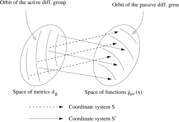
Figure 10: The relation between active and passive diffs and the choice of coordinates.

In order to avoid confusion with regard to passive and active diffeomorphisms in coordinate-dependent considerations, we simply drop coordinates and pass over to the coordinate-free formulation. Thus we consider the manifold $\mathcal{M}$ with metric $g$, defined as the map

$$g:\mathcal{M}\times\mathcal{M} \rightarrow \mathbb{R}$$ (78)

$$\left(P,Q\right) \mapsto d_{g}\left(P,Q\right)\;,$$ (79)

where $P,Q\in\mathcal{M}$. Suppose $d_{g}$ solves Einstein’s equations. A diffeomorphism $\phi:\mathcal{M}\rightarrow\mathcal{M}$ acts as a smooth displacement over the manifold, resulting in $d_{\tilde{g}}$,

$$d_{\tilde{g}}\left(P,Q\right)=d_{g}\left(\phi^{-1}(P),\phi^{-1}(Q)\right)\;.$$ (80)

Active diffeomorphism invariance is the fact that if $d_{g}$ is a solution of the Einstein theory, so is $d_{\tilde{g}}$. This shows that Einstein’s theory is invariant under (active!) diffeomorphisms even in a coordinate free formulation.

General relativity is distinguished from other dynamical field theories by its invariance under active diffeomorphisms. Any theory can be made invariant under passive diffeomorphisms. Passive diffeomorphism invariance is a property of the formulation of a dynamical theory, while active diffeomorphism invariance is a property of the dynamical theory itself. Invariance under smooth displacements of the dynamical fields holds only in general relativity and in any general relativistic theory. It does not hold in QED, QCD, or any other theory on a fixed (flat or curved) background.

4.2 Dirac Observables

Consider a classical dynamical system whose equations of motion do not uniquely determine its evolution, as pictorially illustrated in Fig. 11. The two solutions $\varphi\,(t)$ and $\tilde{\varphi}\,(t)$ which evolve from the same set of initial data, separate at some later time $\hat{t}$, i.e.

$$\varphi\,(t) = \tilde{\varphi}\,(t)\hskip 17.07164pt\mbox{if}\hskip 17.07164ptt<\hat{t}$$ (81)

$$\varphi\,(t) \neq \tilde{\varphi}\,(t)\hskip 17.07164pt\mbox{if}\hskip 17.07164ptt\geq\hat{t}\geq 0\;.$$ (82)

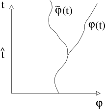
Figure 11: An example for a not uniquely determined evolution of a dynamical system.

Then, as first accurately argued by Dirac, $\varphi\,(t)$ and $\tilde{\varphi}\,(t)$ must be physically indistinguishable or gauge-related, respectively. Otherwise determinism, which is a basic principle in classical physics, would be lost. Dirac gave the definition of observables respecting determinism in the following way. A gauge invariant or Dirac observable is a function $\mathcal{O}$ of the dynamical variables that does not distinguish $\varphi\,(t)$ and $\tilde{\varphi}\,(t)$, i.e.

$$\mathcal{O}\big{(}\varphi\,(t)\big{)}=\mathcal{O}\big{(}\tilde{\varphi}\,(t)\big{)}\;.$$ (83)

In other words, only those observables that have the same values on the solutions $\varphi\,(t)$ and $\tilde{\varphi}\,(t)$ can be observed. Hence the theory can predict only Dirac observables.

Does this imply that any physical quantity that we measure is necessarily a Dirac observable? It turns out that the answer is in the negative. To understand this sublety, consider the example of a simple pendulum described by the variable $\alpha$ which is the deflection angle out of equilibrium. The motion of the pendulum is given by the evolution of $\alpha$ in time $t$, namely by $\alpha(t)$. Since $\alpha(t)$ is predicted by the equation of motion for any time $t$ once the initial data set is fixed, it is a Dirac observable. One should notice that we are actually describing a system in terms of two physical quantities rather than one, namely the pendulum itself, described by position $\alpha$, and a clock measuring the time $t$. However, in contrast to position at a given time, there is no way how time itself could be “predicted”. It simply tells us “when” we are. Therefore, $t$ is a measureable quantity but it is not a Dirac observable. To state this more precisely, we introduce the notion of partial observables. We call $t$ an independent partial observable and $\alpha$ a dependent partial observable. The Dirac observable is given by $\alpha(t)$.

There is an important relation between Dirac observables and the Hamitonian formalism. Dirac observables are characterized by having vanishing Poisson brackets with the constraints. In fact, the entire constrained system formalism was built by Dirac with the purpose of characterizing the gauge invariant or Dirac observables, respectively. To elucidate this feature, consider a classical dynamical system with canonical Hamiltonian $H_{0}$, as well as $k$ additional constraints

$$C_{m}=0\;,\hskip 17.07164ptm=1,\dots,k\;,$$ (84)

defined on phase space. The complete Hamiltonian, which is defined on the full phase space, is then given by

$$H=H_{0}+N_{m}(t)\,C_{m}\;,$$ (85)

with $k$ arbitrary functions $N_{m}(t)$. The dynamics of an observable $\mathcal{O}$ is given by the Hamilton’s equations

$$\frac{d\mathcal{O}}{dt}=\{\mathcal{O},H\}+N^{m}(t)\{\mathcal{O},C_{m}\}\;.$$ (86)

From this one recognizes immediately that the evolution is deterministic, and thus $\mathcal{O}$ a Dirac observable, only if

$$\{\mathcal{O},C_{m}\}=0\hskip 28.45274pt\forall\;m\;,$$ (87)

just as claimed before.

4.3 The Hole Argument

Dirac’s postulate that only gauge invariant or Dirac observables, respectively, can be measurable quantities, was applied to general relativity by Einstein himself in his famous “hole argument” from 1912, cf. [42].

Suppose we have a space–time $\mathcal{M}$ including other structures that represent matter (e.g. scalar fields or particles). Suppose furthermore that the matter configuration is such that there is a hole in space–time, i.e. a region without matter, as indicated in Fig. 12. Let $g_{\mu\nu}(x)$ and $\tilde{g}_{\mu\nu}(x)$ be two distinct metrics which are equal everywhere in $\mathcal{M}$ except for the hole, but nevertheless, both are supposed to solve Einstein’s equations. Now we introduce a spacelike (initial data) surface such that the hole is entirely in the future of it. Since the metrics are equal everywhere outside, they do have the same set of initial data on the surface.

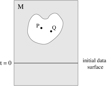
Figure 12: The hole argument.

If we now consider the distance $d$ between two distinct points $P$ and $Q$ which are both inside the hole, we note immediately that $d_{g}(P,Q)\neq d_{\tilde{g}}(P,Q)$, although the metrics have the same inital conditions. Hence, according to the discussion in the previous section, $d_{g}$ is not a Dirac observable. So it seems that we uncovered a mystery of the theory! The distance is not an observable predicted by the theory. Then the obvious question we have to ask is:

“What is predicted by general relativity at all?”

Einstein was so impressed by this conclusion, that he claimed in 1912 that general covariance could not be a property of the theory of gravity. It took some time—three years—until Einstein presented the solution to this puzzle, and thus got back to general covariance, in 1915. To illustrate his strategy, we consider a setting similar to the one above, which corresponds to Fig. 12. More precisely, we consider general relativity and 4 particles denoted as $A,B,C$ and $D$. Their trajectories are determined by the equations of motion and they are supposed to start at the spacelike inital surface, as shown in Fig. 13. Furthermore, we suppose that $A$ and $B$ meet in $i$ inside the hole, and $C$ and $D$ meet in $j$ inside the hole as well. Consider now the distance $d$ between the point $i$ and the point $j$. Is $d$ a Dirac observable? At first sight, we are in the same situation as above, but there is an essential subtle difference in the way we have defined the observable. Consider now the diffeomorphism that sends $g_{\mu\nu}(x)$ into $\tilde{g}_{\mu\nu}(x)$. Since the theory is invariant only under a diffeomorphism that acts on all its dynamical variables, $\tilde{g}_{\mu\nu}(x)$ is a solution of the Einstein equations only if the diffeomorphism displaces the trajectories of the particles as well. Thus $i$ and $j$ will also be displaced by the diffeomorphism. Then, after having performed the active diffeomorphism, the new distance between the intersection points is

$$\tilde{d}=d_{\tilde{g}}\big{(}\phi(i),\phi(j)\big{)}=d_{g}\big{(}\phi^{-1}\phi(i),\phi^{-1}\phi(j)\big{)}=d_{g}(i,j)=d\;.$$ (88)

Hence it follows that this distance is gauge invariant. The distance $d$ between the intersection points is indeed a Dirac observable.

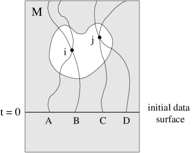
Figure 13: A solution to the hole argument.

One can extend this setting also to cases which involve fields. As an example, consider general relativity and 2 additional fields, namely $g_{\mu\nu}(x)$, $\varphi_{t}(x)$, and $\varphi_{z}(x)$. Then the area $\mathfrak{A}$ of the $\varphi_{t}=\varphi_{z}=0$ surface is a Dirac observable as well, and is given by

$${\mathfrak{A}}=\int_{\varphi_{t}=0\atop\varphi_{z}=0}d^{2}\sigma\,\sqrt{\det{}^{2}g}\;.$$ (89)

As a slightly generalized example, consider general relativity and three fields, i.e. $g_{\mu\nu}(x)$, $\varphi_{t}(x)$, $\varphi_{z}(x)$, and $\varphi_{\scriptscriptstyle\Sigma}(x)$, the area ${\mathfrak{A}}(\Sigma)$ of the surface determined by

$$\varphi_{t}=\varphi_{z}=0,\;\;\mbox{and}\;\;\varphi_{\scriptscriptstyle\Sigma}\geq 0$$ (90)

is given by

$${\mathfrak{A}}(\Sigma)=\int_{\varphi_{t}=0\atop\varphi_{z}=0}d^{2}\sigma\,\delta(\varphi_{\scriptscriptstyle\Sigma})\,\sqrt{\det{}^{2}g}\;.$$ (91)

The reader can convince herself that a diffeomorphism transforming all the fields $\big{(}g_{\mu\nu}(x),\varphi_{t}(x),\varphi_{z}(x),\varphi_{\scriptscriptstyle\Sigma}(x)\big{)}$ does not change the number ${\mathfrak{A}}(\Sigma)$. Thus ${\mathfrak{A}}(\Sigma)$ is a Dirac observable.

In general, to define “local” Dirac observables in general relativity we have to use some of the degrees of freedom of the theory (the particles, the fields) for localizing a space–time point or a space–time region. It is important to notice that in principle we do not need matter or fields to do so. Instead, we can use part of the degrees of freedom of the graviational field itself. This strategy was followed for instance by Komar and Bergman by defining 4 curvature scalars and using them as physically defined coordinates [43]. While formally correct, the use of gravitational degrees of freedom for defining observables in general relativity leads us far away from observables concretely used in realistic applications of general relativity, all of which use matter degrees of freedom for localizing the observables. An example of a realistic observable used in physical applications of general relativity is the physical distance between two space–time events, one on a Global Positioning System (GPS) satellite and one on a Earth based GPS station. In this case, matter degrees of freedom (coupled to gravity) localize two space–time points and the distance between them is a Dirac observable.

To sum up, we have seen that the puzzle of the hole argument can be resolved. Physical quantities predicted by general relativity, i.e. Dirac observables, can be defined inside the hole. But in order to “localize” points, we have to use some dynamical quantity. The most realistic way of doing so is to use matter. In other words, Dirac observables are defined in space–time regions which are determined by dynamical objects.

In the following section, we will see that this definition of localization, which is necessary in general relativity, implies a profound change of our notions of space and time.

4.4 The Physical Interpretation

Before considering the conceptual changes in the notions of space and time brought by general relativity, it is instructive to reflect on the main modifications that these concepts have undergone in the historical development of physics. The key developments in this business are related to the names of Descartes (and Aristotle), Newton, and last but not least, Einstein.

According to Descartes, there is no “space” at all, but only physical objects which can be in touch with each other. The “position” or location, respectively, of an object is only defined by the naming of other physical objects close to it, i.e. the position of a body is the set of those objects to which the body is contiguous. Equally important is the concept of “motion”, which is defined as the change of position. Thus motion is determined by the change of contiguity, i.e. only in relation to other objects. This point of view is denoted as relationalism. Descartes’ definitions of space, position, and motion are by the way essentially the same that were given by Aristotle.

An important historical step was then provided by Newton’s definition of physical space. According to Newton, “space” exists by itself, independently of the objects in it. Motion of a body can be defined with respect to space alone, irrespectively whether other objects are present. Newton insists on this points, on the ground that acceleration can be defined absolutely. In fact, it is only thanks to the fact that acceleration is defined in absolute terms, that the entire structure of Newton’s mechanics ($F=ma$) holds. Newton discussed the fact that acceleration is absolute in the famous example of the rotating bucket, which shows that the absolute rotation of the water, and not the rotation with respect to the bucket, has observable consequences. Thus, according to Newton, space exists independently of objects, weather they are present or not. The location of objects is the part of space that they occupy. This implies that motion can be understood without regard to surrounding objects. Similarly, Newton uses absolute time, leading to a space–time picture which provides an always present fixed background over which physics takes place. Objects can always be localized in space and time with respect to this fixed non-dynamical background.

But if there is “space” which is always present, how can it be captured, or observed? This can be done by using reference systems. The great idea was to select some physical bodies (like walls, rules or clocks) and treat them as reference systems. Physically one has to distinguish the dynamical objects that one wants to study from reference system objects. They are dynamically decoupled.

In the language introduced earlier, the dynamical objects define dependent partial observables, while the objects referred to as reference system define independent partial observables. Examples of dynamical objects may be the deflection angle $\alpha$ of a pendulum, or the position $\vec{x}$ of a particle. An example of a reference system variable is the clock time $t$. The Dirac observables would then just be $\alpha(t)$ and $\vec{x}(t)$.

As an example, we consider the case of a pendulum. The differential equation governing this dynamical system is (for small oscillations) just $\ddot{\alpha}(t)=-\omega^{2}\,\alpha(t)$. The solution is

$$\alpha(t)=A\sin(\omega t+\varphi)\;.$$ (92)

A state is determined by the constants $A$ and $\varphi$, or equivalently, by initial position and velocity at some fixed time. Once the state (i.e. $A$ and $\varphi$) is known, the functional dependence $\alpha(t)$ between the dependent and independent observables can be computed. In fact, it is given by (92).

Thus, in the Newtonian scheme, we have a fixed space and a fixed time, revealed by the objects of the reference system. The objects forming the reference system determine localization in space and in time and define partial observables ($t$, above) which are not dynamical variables in the dynamical models one considers.

In general relativity things change profoundly. We have seen in the discussion of the hole argument and its solution, that the theory does not distinguish reference system objects from dynamical objects. This means that independent and dependent physical observables are not distinguished any more! The reference system can not be decoupled from the dynamics. Therefore, in the Einsteinian framework the notion of “dynamical object” has to be extended compared to the Newtonian case, since now also the reference system objects are included as dynamical variables. Localization of observables is determined by other variables of the theory. Therefore:

Position and Motion are fully relational in General Relativity!

This important statement is the same as provided in the Cartesian–Aristotelian picture.

The essential consequence of the fact that localization of dynamical objects in general relativity is defined only with respect to each other, is the appearance of the diffeomorphism group. Indeed, if we displace all dynamical objects in the manifold at once, we generate nothing but an equivalent mathematical description of the same physical state, because localization with respect to the manifold is irrelevant. In other words, the individual mathematical points in the manifold have no intrinsic physical significance. Only relative localization is relevant. This is precisely the claim of active diffeomorphism invariance of the theory. Hence, a physical state is not located somewhere.

In a quantum theory of gravity, we should not expect quantum exitations on space–time, as the Newtonian point of view would imply, rather we should expect quantum excitations of space–time.

The challenge in the construction of quantum gravity is to find a quantum field theory in which position and motion are fully relational, i.e. a quantum field theory without an a priori space–time localization. Here the wheel turns full circle, and we return to loop quantum gravity, which implements precisely these requirements.

5 Dynamics, True Observables and Spin Foams

The analysis of the important question of observability in general relativity led to the insight that spatiotemporal relationalism à la Descartes plays a major role in the formulation of the theory.

In this section we will return to the quantum theory and firstly focus on the implementation of relationalism into the framework of canonical quantum gravity. Secondly, we will investigate the dynamics and the true, i.e. physical observables of the theory, which formally amounts to the still open problem of solving the Hamiltonian constraint. Instead of attacking this directely, we will construct a projection operator onto the physical states of loop quantum gravity, which will lead to a covariant space–time formulation and a relation to the so-called spin foam models. For a more detailed analysis of this topic we refer to [44].

As we mentioned at the end of the last section, loop quantum gravity is well-suited to tackle the matters discussed there. Thus, the starting point of our considerations is the implementation of the concept of non-localizability into the framework of loop quantum gravity. And of course, as one might have expected, this is achieved by solving the diffeomorphism constraint!

Recall from sect. 2.5 that the basis in the gauge invariant Hilbert space $\mathcal{H}_{0}$ is given by the spin network states $\Psi_{S}(A)$. In the following we adopt Dirac’s bra-ket notation and denote an abstract basis state $\Psi_{S}$ as $|S\rangle$, such that a state in the connection representation would be given by

$$\Psi_{S}(A)=\langle A|S\rangle\;.$$ (93)

5.1 The Diffeomorphism Constraint

In sect. 2.3.3 we have shown that the Hilbert space $\mathcal{H}$ carries a natural unitary representation $U(Diff)$ of the diffeomorphism group $Diff(M)$ of the 3-manifold $M$,

$$U(\phi)\,\Psi(A)=\Psi(\phi^{-1}A)\;,\hskip 28.45274pt\phi\in Diff(M)\;.$$ (94)

In the following we will outline the construction of the diffeomorphism invariant Hilbert space $\mathcal{H}_{diff}$ (recall Fig. 2), which can be considered as the space $\mathcal{H}/Diff(M)$ of solutions of the quantum diffeomorphism contraint.

Let us now consider a finite action of a $U(Diff)$ on a spin network state $|S\rangle$. We get

$$U(\phi)|S\rangle=|\phi\cdot S\rangle\;.$$ (95)

Thus, $U$ sends a state of the spin network basis to another one which is based on a shifted graph. To obtain states which are invariant under $U$, one has to solve

$$U\Psi=\Psi\;.$$ (96)

However, there is no finite norm state invariant under the action of the diffeomorphism group. This is not surprising, since the gauge group is not compact, and leads us to a familiar situation in quantum theory. The way out is to use generalized state techniques. The simplest manner of doing so is (roughly) to solve (96) in $\mathcal{H}^{*}$, the topological dual of the space of finite linear combinations of spin network states. We construct $\mathcal{H}_{diff}$ as the $Diff(M)$ invariant part of $\mathcal{H}^{*}$.

Let $s$ be an equivalence class of embedded spin networks $S$ under the action of $Diff(M)$, i.e. $S,S^{\prime}\in s$, if there exists a $\phi\in Diff(M)$, such that $S^{\prime}=\phi\cdot S$. An equivalence class $s$ or abstract spin network, respectively, is a spin network which is “smeared” over $M$. It is usually called $s$-knot. For each of these $s$-knots an element $\langle s|$ of $\mathcal{H}_{diff}$ is defined. Since they lie in a subset of the dual of $\mathcal{H}$, they act naturally on spin network states as

$$\langle s|S\rangle=\left\{\begin{array}[]{c@{\qquad}l}0&\mbox{if\quad}S\not\in s\\ \vspace{0mm}\hfil&\\ 1&\mbox{if\quad}S\in s\;.\end{array}\right.$$ (97)

A scalar product in $\mathcal{H}_{diff}$ is defined by

$$\langle s|s^{\prime}\rangle=c(s)\,\delta_{ss^{\prime}}\;.$$ (98)

Here $c(s)$ is the (discrete) number of isomorphisms of an $s$-knot into itself, that preserve the coloring and can be obtained from a diffeomorphism of $M$. One can prove [33] that self-adjoint and diffeomorphism invariant operators in $\mathcal{H}_{0}$ are self-adjoint under this inner product when restricted to $\mathcal{H}_{diff}$. Thus (98) is the appropriate physical scalar product as we claimed in sect. 2.1, picked out by the requirement that real classical quantities become self-adjoint operators. Accordingly, the states $\big{(}1/\sqrt{c(s)}\big{)}|s\rangle$ form an orthonormal basis (notice that we freely interchange bra’s and ket’s).

The states $|s\rangle$ are the (3d) diffeomorphism invariant quantum states of the gravitational field. They are labelled by abstract, non-embedded (knotted, colored) graphs $s$, the $s$-knots. As we have seen above, each link of the graph can be seen as carrying a quantum of area. As shown for instance in [34], a similar results holds for the volume: in this case, that are the nodes that carry quanta of volume. Thus, an $s$-knot can be seen as an elementary quantum excitation of space formed by “chunks” of space (the nodes) with quantized volume, separated by sheets of surface (corresponding to the links), with quantized area. The key point is that an $s$-knot does not live on a manifold. The quantized space does reside “somewhere”. Instead, it defines the “where” by itself. This is the picture of quantm space–time that emerges from loop quantum gravity.

5.1.1 Formal Manipulations.

We close the discussion on the diffeomorphism constraint by reexpressing the diffeomorphism invariant states using some intriguing formal expressions that will lead us to dealing with the Hamiltonian constraint.

Although we noticed that $\mathcal{H}_{diff}$ is not a subspace of $\mathcal{H}$, there exists nevertheless a “projection operator” $\Pi$,

$$\Pi\;:\;\mathcal{H}\rightarrow\mathcal{H}_{diff}\;.$$ (99)

It acts as

$$\Pi|S\rangle=|s\rangle\;,$$ (100)

i.e. a spin network state in $\mathcal{H}$ is mapped to the corresponding diffeomorphism invariant equivalence class in $\mathcal{H}_{diff}$. In the following, we are going to describe its construction. We start by formally defining a measure on $Diff(M)$, which is required to satisfy

$$\int_{Diff}[d\phi]=1\;,$$ (101)

and

$$\int_{Diff}[d\phi]\,\delta_{S,\phi\cdot S}=c(s)\;.$$ (102)

Loosely speaking, (102) refers to taking an embedded spin network, acting with diffeomorphisms on it (i.e. displace it smoothly in the manifold), and finally moving it back to the spin network one started with. Then $c(s)$ just counts the number of ways one can do this.

Now, a diffeomorphism invariant knot state $|s\rangle$ can be written as

$$|s\rangle=\int_{Diff}[d\phi]\,|\phi\cdot S\rangle\;,\hskip 28.45274ptS\in s\;.$$ (103)

Using only the definitions (101)–(103), one can in fact derive (97) and (98). Furthermore, we can also give a more explicit (but still formal) expression of the projection operator $\Pi$. First, note that the generator of the diffeomorphism constraint $\vec{D}[\vec{f}]$, which is a smooth vector field $\vec{f}$ on $M$, is an element of the Lie algebra of $Diff(M)$. Then, from (95) and (103) one concludes

$$|s\rangle=\int_{Diff}[d\phi]\,U(\phi)|S\rangle=\int[d\vec{f}]\,e^{i\vec{f}\vec{D}}\,|S\rangle\;,$$ (104)

where in the second step we have expressed a group element $U(\phi)\in U(Diff)$ as the exponential of an element of the Lie algebra, and formally integrated over the algebra rather that the group. From this and (100) we can immediately read off the projector

$$\Pi=\int[d\vec{f}]\,e^{i\vec{f}\vec{D}}\,.$$ (105)

Finally, we also obtain a diffeomorphism invariant quadratic form on $\mathcal{H}$ via

$$\langle S|S^{\prime}\rangle_{diff}\equiv\langle S|\Pi|S^{\prime}\rangle=\int[d\vec{f}]\,\langle S|e^{i\vec{f}\vec{D}}|S^{\prime}\rangle\;,$$ (106)

where one should notice that the spin networks $S$ and $S^{\prime}$ are itselves not diffeomorphism invariant. Hence it follows (roughly) that the knowledge of the “matrix elements” $\langle S|\Pi|S^{\prime}\rangle$ of the projection operator is equivalent to the solution of the diffeomorphism constraint!

5.2 The Hamiltonian Constraint, Spin Foam and Physical Observables

In Fig. 2 we illustrated the general outline for a step by step construction of the physical Hilbert space by solving the quantum constraint operators one after another. Carrying this out, we were led from the unconstrained Hilbert space $\mathcal{H}$ firstly to the gauge invariant space $\mathcal{H}_{0}$, equipped with an orthonormal basis of spin network states $|S\rangle$, and secondly, as we described in sect. 5.1, to the diffeomorphism invariant Hilbert space $\mathcal{H}_{diff}$, for which it was also possible to define an orthonormal basis $|s\rangle$ of $s$-knot states. The final step, marked with a question mark in Fig. 2, remains to be done: the physical states of the theory should lie in the kernel of the quantum Hamiltonian constraint operator. Of course, we do not expect to find a complete solution of the Hamiltonian constraint, which would correspond to a complete solution of the theory. Rather, we need a well posed definition of the Hamiltonian constraint, and a strategy to compute with it and to unravel its physical content.

Here, we will give only a sketchy account of the definition of the Hamiltonian constraint. On the other hand, we will illustrate the way of using this constraint a bit more in detail. The idea we will illustrate is to search the solution of the constraint by constructing a projector on physical states, using the procedure we described in the last section for the diffeomorphism constraint as a guide to the solution of the Hamiltonian constraint. This construction will lead us to the so-called spin foam models, which represent a covariant formulation of the dynamics of quantum gravity. In the light of recent developments, these models provide the most exciting and promising approach to the subject.

5.2.1 A Simple Example.

We have already considered the construction of a projection operator in relation to the diffeomorphism constraint in sect. 5.1. Nevertheless, it is instructive to give here a simple toy example that should explain the procedure in a more accurate way.

Consider a simple dynamical quantum mechanical system with an unconstrained Hilbert space of square integrable functions over $\mathbb{R}^{2}$, i.e. $\mathcal{H}=L^{2}(\mathbb{R}^{2})$. Let the system be constrained by demanding invariance with respect to rotations around the $z$-axis, i.e by having the angular momentum operator

$$\hat{J} := \hat{J}_{z}=i\,(x\,\partial_{y}-y\,\partial_{x})$$ (107)

$$\widehat{=} \hat{J}_{\varphi}=i\,\partial_{\varphi}$$ (108)

as the quantum constraint. In (107) and (108) we considered two representations, namely the cartesian and the polar coordinate one, in which the wave functions appear as $\Psi(x,y)$ or $\Psi(r,\varphi)$, respectively. We will confine ourselves to the latter one. The physical Hilbert space $\mathcal{H}_{phys}$ is given as the subspace of $\mathcal{H}$ subject to

$$\hat{J}\Psi=0\;,$$ (109)

i.e. the physical state functionals are required to lie in the kernel of the quantum constraint operator $\hat{J}$. We know that $\hat{J}$ is the generator of the group $U(1)$ with parameter $\alpha$, acting as

$$U(1)\times\mathbb{R}^{2} \rightarrow \mathbb{R}^{2}$$ (110)

$$\big{(}\alpha,(r,\varphi)\big{)} \mapsto (r,\varphi+\alpha)\;.$$ (111)

Due to compactness of $U(1)$, the constraint equation (109) could be solved directly. However, we will follow a different path. We try to solve the problem using a projection operator

$$\Pi\;:\hskip 14.22636pt\mathcal{H}\rightarrow\mathcal{H}_{phys}\;.$$ (112)

Note that the (finite) action of the constrait on a general state functional $\Psi(r,\varphi)$ is given by

$$e^{i\alpha\hat{J}}\,\Psi(r,\varphi)=\Psi(r,\varphi+\alpha)\;.$$ (113)

Hence, the projection operator $\Pi$ on physical states is defined as

$$\Pi=\frac{1}{2\pi}\int_{0}^{2\pi}d\alpha\,e^{i\alpha\hat{J}}\;.$$ (114)

It acts on $\Psi(r,\varphi)\in\mathcal{H}$ as follows,

$$\Pi\,\Psi(r,\varphi) = \frac{1}{2\pi}\int_{0}^{2\pi}d\alpha\,e^{i\alpha\hat{J}}\Psi(r,\varphi)$$ (115)

$$= \frac{1}{2\pi}\int_{0}^{2\pi}d\alpha\,\Psi(r,\varphi+\alpha)=\tilde{\Psi}(r)\;,$$ (116)

resulting in a new function $\tilde{\Psi}(r)$ which is independent of $\varphi$, just as one might have expected for the physical states. Applying $\Pi$ a second time proves the correct projector property $\Pi^{2}=\Pi$. However, because of the existence of the projector, there is no need to perform calculations in the physical subspace $\mathcal{H}_{phys}$, rather one can stay in the unconstrained Hilbert space $\mathcal{H}$—a remarkable simplification! Using the scalar product

$$\langle\Psi|\Phi\rangle=\int_{0}^{2\pi}\!\!\int_{0}^{\infty}\!d\varphi\,dr\>\overline{\Psi(r,\varphi)}\,\Phi(r,\varphi)$$ (117)

in $\mathcal{H}$, one arrives at the important result

$$\langle\Psi|\Phi\rangle_{phys}\equiv\langle\Psi|\Pi|\Phi\rangle\;.$$ (118)

This equation is similar to the result obtained in the discussion of the diffeomorphism constraint in sect. 5.1. The quadratic form $\langle\,|\,\rangle_{phys}$ in $\mathcal{H}_{phys}$ is indeed expressed as a scalar product over states which lie in $\mathcal{H}$. Thus, knowing the matrix elements (118) of the projection operator in the unconstrained Hilbert space is equivalent to having solved the constraint!

It is worth mentioning, that a similar scheme can be applied to operators. Suppose there exists a non gauge invariant operator $O=O(r,\varphi)$ on $\mathcal{H}$. Then a fully gauge invariant operator $R=R(r)$ in $\mathcal{H}_{phys}$ can be constructed by defining

$$R:=\Pi\,O\,\Pi\;.$$ (119)

The calculation of matrix elements of the physical operator $R$ is then reduced to a calculation in the unconstrained Hilbert space, which gives

$$\langle\Psi|O|\Phi\rangle_{phys}\equiv\langle\Psi|\Pi\,O\,\Pi|\Phi\rangle\;.$$ (120)

5.2.2 The Hamiltonian Constraint.

Let us now proceed with the application of the projector method to the Hamiltonian constraint in quantum gravity, the only and least understood constraint which still remains to be solved in order to describe the dynamics of the theory. The following discussion is mainly based on plausibility considerations resulting in rough arguments. A more complete treatment would include exponentially increasing efforts, which lies beyond the scope of this lecture.

The Lorentzian Hamiltonian constraint can be written as the sum of two terms, where one is the Euclidean Hamiltonian constraint. Here, we deal for simplicity only with this Euclidean part, which means that we actually consider Euclidean gravity only. Classically, the constraint reads roughly

$$H_{cl}\simeq F_{ab}E^{a}E^{b}+\mbox{Lorentzian part}\;.$$ (121)

$E^{a,b}$ are the triads, and $F_{ab}$ is the curvature of the connection, which, we recall, is an antisymmetric tensor.

When passing over to the quantum theory, $H_{cl}$ is promoted to an operator which has to be suitably regularized. A typical regularization process consists of the following steps. First, introduce a regularization parameter $\epsilon$, and replace the classical expression (121) with a regularized, $\epsilon$ dependent one, written in terms of quantities that we know how to promote to quantum operators, and which tend to $H_{cl}$ as $\epsilon$ tends to zero. In particular, $F$ is replaced by the holonomy of an $\epsilon-$size loop. In the second step, replace the classical quantities with their quantum analogues leading to the Hamiltonian operator $\hat{H}_{\epsilon}$. Finally, the parameter is forced to go to zero, $\epsilon\rightarrow 0$, yielding a well-defined quantum Hamiltonian operator $\hat{H}_{\epsilon}\rightarrow\hat{H}$.

We will not carry out this construction explicitely but only mention that there exist several different versions. The first completely consistent construction, yielding a well-defined and finite operator, was obtained by Thiemann in [25].

However, the key point which is common to all different regularization procedures is the vanishing of the action of the Hamiltonian operator on the holonomy $U[A,\gamma]$. That is

$$\hat{H}(x)\,U[A,\gamma]=0\;,$$ (122)

if $x$ is on an interior point of the curve $\gamma$. The reason for this can roughly be understood as follows. If we replace the triad in (121) with its quantum analogue and apply the resulting operator to the holonomy (without bothering about regularization), we obtain

$$F_{ab}\,\frac{\delta}{\delta A_{a}}\frac{\delta}{\delta A_{b}}\,U[A,\gamma]\;\sim\;F_{ab}\,\dot{\gamma}^{a}\dot{\gamma}^{b}=0\;.$$ (123)

While $F_{ab}$ is an antisymmetric tensor, the product of $\dot{\gamma}^{a}$ and $\dot{\gamma}^{b}$, which are tangent to $\gamma$, is, on the other hand, symmetric. Thus the result is zero, since we contract an antisymmetric tensor with a symmetric quantity. This derivation has only a formal character since an infinite coefficient multiplies the right hand side of (123). Anyhow, a careful calculation using rigorous regularization yields the same result.

However, calculating the action of $\hat{H}$ on spin network states, the result turns out to be not equal to zero,

$$\hat{H}(x)\,\Psi_{S}\neq 0\;.$$ (124)

This fact is due to the end points of the links, i.e. the nodes of the spin network. At a node, the tangent vectors $\dot{\gamma}^{a}$ and $\dot{\gamma}^{b}$ in (123) might refer to distinct links adjacent to the node. This results in terms with non-zero contributions. Hence one concludes that the Hamiltonian constraint operator acts on the nodes only.

The result of the action of $\hat{H}$ on a spin network state $|S\rangle$ turns out to be given by

$$\hat{H}[N]\,|S\rangle=\sum_{\mbox{\scriptsize nodes}\,n\,\mbox{\scriptsize of}\,S}A_{n}\,N(x_{n})\,\hat{D}_{n}\,|S\rangle\;,$$ (125)

where $x_{n}$ refers to the point in which the node $n$ is located. The action of the operator $\hat{D}_{n}$ is illustrated in Fig. 14. An extra link with color one connecting two points $p_{1}$ and $p_{2}$ lying on distinct links adjacent to the node $p$ is created when acting on a single node. The color of the link between $p$ and $p_{1}$, as well as between $p$ and $p_{2}$ is altered and the state is multiplied by a coefficient $A$. Explicit expressions are computed in [45]. Moreover, $\hat{H}[N]$ is the Hamiltonian constraint smeared with a scalar function $N(x)$ given by

$$\hat{H}[N]=\int d^{3}x\,N(x)\,\hat{H}(x)\;.$$ (126)

Figure 14: The action of the Hamiltonian constraint on a trivalent node.

5.2.3 Spin Foam.

Now we want to define the physical Hilbert space $\mathcal{H}_{phys}$ using the projector method explained above, starting from the diffeomorphism invariant Hilbert space $\mathcal{H}_{diff}$ by considering $s$-knot states. Similar to (105) or (114), respectively, we construct the projection operator

$$P=\int[dN]\,e^{i\hat{H}[N]}=\int[dN]\,e^{i\int N\,\hat{H}}\;.$$ (127)

In the abstract spin network basis, the matrix elements of $P$ are

$$\langle s|P|s^{\prime}\rangle=\langle s|\int[dN]\,e^{i\int N\,\hat{H}}|s^{\prime}\rangle\;.$$ (128)

It can be shown, that a diffeomorphism invariant notion of integration exists for this functional integral [44]. According to (106) or (118), respectively, we use the matrix elements of the projector to define the quadratic form

$$\langle s|s^{\prime}\rangle_{phys}=\langle s|P|s^{\prime}\rangle\;.$$ (129)

The physical Hilbert space $\mathcal{H}_{phys}$ is then defined over $\mathcal{H}_{diff}$, from which we started, via this quadratic form.

In order to calculate the matrix elements (128) of the projector, the exponent is expanded. Neglecting many technicalities which are given in [46] the expansion looks schematically as follows,

$$\langle s|P|s^{\prime}\rangle\sim\langle s|s^{\prime}\rangle+\int[dN]\,\left(\langle s|\hat{H}|s^{\prime}\rangle\ +\langle s|\hat{H}\hat{H}|s^{\prime}\rangle\ +\ldots\right)\;.$$ (130)

Using now the action (125) of $\hat{H}$ on spin network states, we obtain

$$\langle s|s^{\prime}\rangle_{phys}=\langle s|P|s^{\prime}\rangle\sim\langle s|s^{\prime}\rangle+\sum_{\mbox{\scriptsize nodes}\,n\,\mbox{\scriptsize of}\,s^{\prime}}A_{n}\,\langle s|s^{\prime}_{n}\rangle+\ldots\;,$$ (131)

where we “integrated out” integrals of the type

$$\int[dN]\,\big{(}N(x_{1})\cdots N(x_{n})\big{)}\;.$$ (132)

Equation (131) admits an extremely compelling graphical interpretation as a sum over histories of evolutions of $s$-knot states. This reveals the meaning of the projector as a propagator in accordance with Feynman.

To see this more clearly, consider the 4-manifold $\mathcal{M}=\Sigma\times[0,1]$. The hypersurfaces at the boundary of $\mathcal{M}$, corresponding to the values $0$ and $1$ in the interval, are denoted as $\Sigma_{i}$ and $\Sigma_{f}$, respectively. We define the “initial state” on $\Sigma_{i}$ as $s_{i}:=s^{\prime}$, and the “final state” on $\Sigma_{f}$ as $s_{f}:=s$. Then the term $\langle s_{f}|s_{i}\rangle$, which is of order zero in the expansion (131), is non-vanishing only if $s_{f}=s_{i}$. In other words, the corresponding graphs have to be continuously deformable into each other such that the colors of the links and nodes match. Graphically, this is expressed by sweeping out a surface $\sigma=\sigma_{i}\times[0,1]$, as shown in Fig. 15. The surface is formed by 2-dimensional submanifolds of $\mathcal{M}$—so-called faces—which join in edges. The faces are swept out by spin network links, and the edges by the nodes. Thus every face of $\sigma$ is colored just as the underlying link, and to every edge the intertwiner of the underlying node is associated.

Figure 15: The diagram corresponding to a term of order zero.

Figure 16: A first order diagram.

Next, we consider a first order term $\langle s|s^{\prime}_{n}\rangle$ in the expansion (131). These term appear as the result of a single action of the Hamiltonian constraint, i.e. they correspond to adding (or removing) one link, or, equivalentely, two nodes into a spin network, cf. Fig. 14. The situation is similar to the one described for the term of order zero, but now at some point $p$ of $\sigma$ the surface branches as shown in Fig. 16. Thus the graph of $s_{i}$ is not equal to the one which is associated to $s_{f}$ any more, as opposed to the previous case. The surfaces are again colored corresponding to the underlying links.

The picture one should have in mind is the following. $\mathcal{M}$ can be imagined as a space–time, and $s_{i}$ is a spin network that evolves continuously in a coordinate denoted as “time” up to a point $p$ where the spin network branches because of the action of the Hamiltonian constraint. At a branching point the single node $p_{i}$ degenerates in the sense of being transformed into three nodes, each distinct pair being connected by a link. The accompanying branching of the surface in $p$ is called the elementary vertex of the theory. It is the simplest geometric vertex, see Fig. 17.

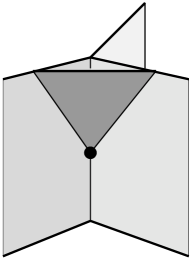
Figure 17: The elementary vertex.

Finally, we will have a closer look to a second order term. In this example we give the coloring of the surfaces as explicitely shown in Fig. 18.

Figure 18: A term of second order.

Consider the transition from an (abstract) spin network $s_{i}$ with two trivalent nodes connected by three links with colors $(3,5,7)$ to the $s$-knot $s_{f}$ with the same underlying graph but different coloring $(3,6,8)$. There an intermediate state with four nodes emerges, such that an elementary creation as well as an elementary annihilation vertex occur giving rise to the coloring specified in Fig. 18. Although our considerations are extremely simplified, it is nevertheless plausible to write the expansion (131) of $\langle s|P|s^{\prime}\rangle$ as a sum over topologically inequivalent branched colored surfaces $\sigma$ bounded by $s_{i}$ and $s_{f}$. These surfaces are called spin foams [46, 47]. Each surface $\sigma$ represents the history of the initial $s$-knot state. It is weighted by the product of coefficients $A_{\nu}$, which are associated to the vertices of $\sigma$. Recall that these coefficients showed up in (125) as a result of the action of the Hamiltonian constraint on $s$-knot states. They depend only on the coloring of the faces and edges adjacent to the relevant vertices. In the end, we obtain

$$\langle s|s^{\prime}\rangle_{phys}=\langle s|P|s^{\prime}\rangle=\sum_{\mbox{\scriptsize spin}\atop\mbox{\scriptsize foams}\,\scriptstyle\sigma}\prod_{\mbox{\scriptsize vertices}\atop\scriptstyle\nu\in\sigma}A_{\nu}\;$$ (133)

for the transition amplitude between the two (abstract) spin network states $s_{i}$ and $s_{f}$. It is designated as a transition amplitude because of the obvious formal analogy to the expressions in standard quantum field theory, giving rise to the interpretation of Fig. 15, 16 and 18 roughly as “Feynman diagrams” of quantum gravity.

This interpretation is reinforced by a number of independent results. For instance, certain discretized covariant approaches to quantum gravity lead precisely to a “sum over discretized 4-geometries”, very similar to (133), cf. [49]. Inspired by the construction above, Baez has defined a general notion of spin foam model and studied the structure of these models in general. See [47, 48] and references therein.

5.2.4 Physical Observables.

To round off this section, we briefly comment on an application of the projector method to the calculation of physical observables. As before, we will not consider problems that arise with normalization, or ill-defined expressions that might occur, but rather concentrate on the conceptual framework. For a more detailed account to this subject we refer to [44].

Trying to construct physical observables, i.e. self-adjoint operators which are invariant under the 4-dimensional diffeomorphism group is a well-known difficulty in (quantum) general relativity. Instead, as explained in the last sections, we can immediately define a fully gauge invariant observable by starting from an operator $O$ acting on $\mathcal{H}_{diff}$, which is invariant under 3-dimensional diffeomorphisms. Using what we noticed in (119), the fully gauge invariant operator $R$ is given by

$$R=P\,O\,P\;.$$ (134)

The projector $P$ onto the physical Hilbert space is defined in (127). Indeed, $R$ is invariant under 4-dimensional diffeomorphisms. Thus, the expectation value in a physical state is

$$\langle s|O|s\rangle_{phys}:=\langle s|P\,O\,P|s\rangle\;.$$ (135)

Doing a similar manipulation of the matrix elements (135) as above, we obtain the expression for the expectation values in the spin foam version as

$$\langle s|O|s\rangle_{phys}\;\sim\sum_{\mbox{\scriptsize spin}\atop\mbox{\scriptsize foams}\,\scriptstyle\sigma}\left(\sum_{\tilde{s}}O(\tilde{s})\right)\prod_{\mbox{\scriptsize vertices}\atop\scriptstyle\nu\in\sigma}A_{\nu}\;.$$ (136)

For simplicity, we have chosen $O$ to be diagonal. Furthermore, $\tilde{s}$ are all possible spin networks that cut a spin foam $\sigma$ (i.e. a branched colored 2-surface) into two parts, a future and a past one. These $\tilde{s}$ may be considered as (ADM-like) spatial slices that cut a given spin foam.

A closer examination of (136) reveals that the first summation has to be performed over all possible spin foams $\sigma$. On top of that, for each of these spin foams, all of its spatial slices have to be summed up. Without going into details, we briefly mention its appealing geometrical interpretation as an “integration over space–time”, or more precisely, as an “integration” over the location of the ADM surfaces in (the quantum version of classical) 4-dimensional space–time. Thus, expectation values of physical observables are given as averages over the spin foam in an intuitively similar manner as one is used to from standard quantum field theory. Moreover, this method provides a framework for the non-perturbative, space–time covariant formulation of a diffeomorphism invariant quantum field theory.

However, so far we haven’t mentioned any problems that arise. Recall first, that we considered only the Euclidean part of the Hamiltonian constraint. Furthermore, it is still unclear what shape physical observables $O$, which are at least required to yield finite results, should take. Intuitively, we might expect that observables of the form

$$O=\tilde{O}\times\delta(\mbox{\footnotesize something})\;,$$ (137)

might be finite, and might correspond to the realistic relational observables discussed above.

But so far the problem of finding physical observables in quantum gravity is still very little explored territory, and our considerations may at best give some vague ideas of what remains to be done.

6 Open Problems and Future Perspectives

This series of lectures was devoted to loop quantum gravity, a non-perturbative canonical formulation for a quantum theory of gravitation. We introduced the basic principles of the theory in the kinematical regime, including spin network states which provide an orthonormal basis in the gauge invariant Hilbert space. As an application, one of the most exiting results obtained in the last few years, the discreteness of geometry, was examined by considering the quantization of the area. Furthermore, by taking the basic principles of general relativity seriously, we have shown by discussing the topics of diffeomorphism invariance and observability in general relativity, that loop quantum gravity is well-adapted for a quantum theory of gravitation.

Finally, in order to examine also the non-perturbative dynamics of quantum gravity a little, an ansatz for the construction of the physical Hilbert space by means of a projection method was explained. We tried to clarify its interpretation in terms of a spin foam model, in which the projection operator itself plays the role of a propagator for the space–time evolution of (abstract) spin networks. Its Feynman diagram like graphic representation was presented as well. We also gave the prospects for a possible calculation of expectation values of operators representing physical observables, by using the spin foam formalism.

There are several open questions which remain to be explored. We mentioned that, because of different regularization schemes, there exist several versions of the Hamiltonian constraint. Thus, one of the most intriguing questions would certainly be to find the “right” consistent Hamiltonian constraint, i.e. the one which has the correct classical limit. Closely related is the question of how such a classical limit should be studied. What are the coherent states? What is the ground state of the theory? Does a notion of “ground state” make sense at all, in a general covariant theory?

The problem of constructing 4-dimensional diffeomorphism invariant observables is crucial. We do know many 4-dimensional diffeomorphism invariant observables in general relativity: in fact, we use them in the classical applications of general relativity, which are nowdays extremely numerous. But to express such observables in the quantum theory is still technically hard. In particular, in order to compare loop quantum gravity with particle physics approaches, and to make contact with traditional quantum field theory, it would be extremely useful to be able to compute scattering amplitudes in an asymptotically flat context. Some kind of perturbation expansion should be used for such a project. But in this context the notion of “expansion”, and “perturbative” are delicate (expand around what?). For these problems, the spin foam formalism may turn out to be essential, since it provides a space–time formulation of a diffeomorphism invariant theory.

We close these lectures by expressing the wish that some of the students that so enthusistically attended them will be the ones able to solve these problems, to give us a fully convincing quantum theory of space–time, and thus push forward this extraordinary beautiful adventure, which is exploring Nature and its marvellous and disconcerting secrets.

References

-
[1]
G. Amelino–Camelia, Gravity wave interferometers as
probes of a low-energy effective quantum gravity.
e-print: gr-qc/9903080.
G. Amelino–Camelia, to appear in: “Proceedings of the XXXVth Karpacz Winter School on Theoretical Physics: From Cosmology to Quantum Gravity,” Polanica, Poland, Feb. 2–12, 1999. - [2] J. Ellis, N.E. Mavromatos and D.V. Nanopoulos, Search for Quantum Gravity. e-print: hep-th/9905048.
- [3] C. Rovelli, Strings, loops and others: A Critical survey of the present approaches to quantum gravity. In: “15th International Conference on General Relativity and Gravitation (GR15),” Pune, India, Dec. 16-21, 1997, e-print: gr-qc/9803024.
- [4] L. Smolin, to appear in: “Proceedings of the XXXVth Karpacz Winter School on Theoretical Physics: From Cosmology to Quantum Gravity,” Polanica, Poland, Feb. 2–12, 1999.
- [5] L. Smolin, The future of spin networks. e-print: gr-qc/9702030.
- [6] C. Rovelli, Loop Quantum Gravity. Living Reviews in Relativity, 1998-1, http://www.livingreviews.org/ and e-print: gr-qc/9710008.
- [7] C. Rovelli and L. Smolin, Discreteness of Area and Volume in Quantum Gravity, Nucl. Phys. B442 (1995) 593, e-print: gr-qc/9411005; Erratum: Nucl. Phys. B456 (1995) 734.
- [8] P.A.M. Dirac, Lectures on Quantum Mechanics. Yeshiva University, New York, 1964.
- [9] A. Sen, Gravity as a spin system. Phys. Lett. 119B (1982) 89.
- [10] T. Jacobson and L. Smolin, Nonperturbative quantum geometries. Nucl. Phys. B299 (1988) 295.
- [11] A. Ashtekar, C. Rovelli and L. Smolin, Weaving a classical geometry with quantum threads. Phys. Rev. Lett. 69 (1992) 237, e-print: hep-th/9203079.
- [12] A. Ashtekar and C.J. Isham, Representations of the holonomy algebra of gravity and non-abelian gauge theories. Class. Quant. Grav. 9 (1992) 1433, e-print: hep-th/9202053.
- [13] J. Baez, Diffeomorphism invariant generalized measures on the space of connections modulo gauge transformations. In: L. Crane and D. Yetter (eds.), “Proceedings of the Conference on Quantum Topology,” Manhattan, USA, Mar. 24–28, 1993, e-print: hep-th/9305045.
- [14] A. Ashtekar and J. Lewandowski, Differential geometry on the space of connections via graphs and projective limits. J. Geom. Phys. 17 (1995) 191, e-print: hep-th/9412073.
- [15] A. Ashtekar, J. Lewandowski, D. Marolf, J. Mourao and T. Thiemann, Quantization of diffeomorphism invariant theories of connections with local degrees of freedom. J. Math. Phys. 36 (1995) 6456, e-print: gr-qc/9504018.
- [16] C. Rovelli, Black Hole Entropy from Loop Quantum Gravity. Phys. Rev. Lett. 77 (1996) 3288, e-print: gr-qc/9603063.
- [17] K. Krasnov, Geometrical entropy from loop quantum gravity. Phys. Rev. D55 (1997) 3505, e-print: gr-qc/9603025.
- [18] A. Ashtekar, J. Baez, A. Corichi and K. Krasnov, Quantum Geometry and Black Hole Entropy. Phys. Rev. Lett. 80 (1998) 904, e-print: gr-qc/9710007.
- [19] C. Rovelli, Ashtekar formulation of general relativity and loop space nonperturbative quantum gravity: A Report. Class. Quant. Grav. 8 (1991) 1613.
- [20] T. Jacobson, New variables for canonical supergravity. Class. Quant. Grav. 5 (1988) 923.
- [21] Y. Ling and L. Smolin, Supersymmetric Spin Networks and Quantum Supergravity. e-print: hep-th/9904016.
- [22] A. Ashtekar, New variables for classical and quantum gravity. Phys. Rev. Lett. 57 (1986) 2244.
- [23] A. Ashtekar, New Hamiltonian formulation of general relativity. Phys. Rev. D36 (1987) 1587.
- [24] T. Thiemann, Anomaly-free formulation of non-perturbative, four-dimensional Lorentzian quantum gravity. Phys. Lett. B380 (1996) 257, e-print: gr-qc/9606088.
- [25] T. Thiemann, Quantum Spin Dynamics (QSD). Class. Quant. Grav. 15 (1998) 839, e-print: gr-qc/9606089.
- [26] F. Barbero, Real Ashtekar Variables for Lorentzian Signature Space-times. Phys. Rev. D51 (1995) 5507, e-print: gr-qc/9410014.
- [27] C. Rovelli and L. Smolin, Knot theory and quantum gravity. Phys. Rev. Lett. 61 (1988) 1155.
- [28] C. Rovelli and L. Smolin, Loop representation of quantum general relativity. Nucl. Phys. B331 (1990) 80.
- [29] R. De Pietri, On the relation between the connection and the loop representation of quantum gravity. Class. Quant. Grav. 14 (1997) 53, e-print: gr-qc/9605064.
- [30] C. Rovelli and L. Smolin, Spin Networks and Quantum Gravity. Phys. Rev. D52 (1995) 5743, e-print: gr-qc/9505006.
- [31] J. Lewandowski, to appear in: “Proceedings of the XXXVth Karpacz Winter School on Theoretical Physics: From Cosmology to Quantum Gravity,” Polanica, Poland, Feb. 2–12, 1999.
- [32] A. Ashtekar, Mathematical Problems of Non-perturbative Quantum General Relativity. In: J. Zinn-Justin and B. Julia (eds.), “Les Houches Summer School on Gravitation and Quantizations,” Les Houches, France, Jul. 5–Aug.1, 1992. North-Holland, 1995. e-print: gr-qc/9302024.
-
[33]
D. Marolf, The spectral analysis inner product for quantum gravity.
In: R.T. Jantzen, G.M. Keiser and R. Ruffini (eds.), “Proceedings
of the VIIth Marcel Grossmann Conference,” Stanford, USA, Jul. 24–30, 1994.
World Scientific, 1996. e-print: gr-qc/9409036.
D. Marolf, Green’s bracket algebras and their quantization. Ph.D. dissertation, The University of Texas at Austin, 1992.
D. Marolf, Quantum observables and recollapsing dynamics. Class. Quant. Grav. 12 (1995) 1199, e-print: gr-qc/9404053. - [34] R. De Pietri and C. Rovelli, Geometry Eigenvalues and Scalar Product from Recoupling Theory in Loop Quantum Gravity. Phys. Rev. D54 (1996) 2664, e-print: gr-qc/9602023.
- [35] C. Rovelli and P. Upadhya, Loop quantum gravity and quanta of space: a primer. e-print: gr-qc/9806079.
- [36] J. Lewandowski, E.T. Newman and C. Rovelli, Variations of the parallel propagator and holonomy operator and the Gauss law constraint. J. Math. Phys. 34 (1993) 4646.
- [37] S. Fritelli, L. Lehner and C. Rovelli, The complete spectrum of the area from recoupling theory in loop quantum gravity. Class. Quant. Grav. 13 (1996) 2921, e-print: gr-qc/9608043.
- [38] A. Ashtekar and J. Lewandowski, Quantum Theory of Geometry I: Area Operators. Class. Quant. Grav. 14 (1997) A55, e-print: gr-qc/9602046.
- [39] C. Rovelli, What is observable in classical and quantum gravity? Class. Quant. Grav. 8 (1991) 297
- [40] C. Rovelli, Halfway Through the Woods: Contemporary Research on Space and Time. In: J. Earman and J.D. Norton (eds.), “The Cosmos of Science,” University of Pittsburgh Press and Universitäts-Verlag Konstanz, Konstanz, 1997.
- [41] C. Rovelli, Quantum spacetime: what do we know? e-print: gr-qc/9903045.
- [42] A. Einstein and M. Grossmann, Entwurf einer verallgemeinerten Relativitätstheorie und einer Theorie der Gravitation. Zeitschrift für Mathematik und Physik 62 (1914) 225.
- [43] P.G. Bergmann and A. Komar, The coordinate group symmetries of general relativity. Int. Jour. Theor. Phys. 5 (1972) 15.
- [44] C. Rovelli, The projector on physical states in loop quantum gravity. Phys. Rev. D59 (1999) 104015, e-print: gr-qc/9806121.
- [45] R. Borissov, R. DePietri and C. Rovelli, Matrix Elements of Thiemann’s Hamiltonian Constraint in Loop Quantum Gravity. Class. Quant. Grav. 14 (1997) 2793, e-print: gr-qc/9703090.
- [46] M. Reisenberger and C. Rovelli, “Sum over Surfaces” form of Loop Quantum Gravity. Phys. Rev. D56 (1997) 3490, e-print: gr-qc/9612035.
- [47] J.C. Baez, Spin Foam Models. Class. Quant. Grav. 15 (1998) 1827, e-print: gr-qc/9709052.
- [48] J.C. Baez, An Introduction to Spin Foam Models of BF Theory and Quantum Gravity. To appear in: H. Gausterer and H. Grosse (eds.), “Geometry and Quantum Physics,” Lecture Notes in Physics (Springer-Verlag, Berlin), e-print: gr-qc/9905087.
- [49] M.P. Reisenberger, A lattice worldsheet sum for 4-d Euclidean general relativity. e-print: gr-qc/9711052.