Generation of Post-Newtonian Gravitational Radiation
via Direct Integration of the Relaxed Einstein Equations

Abstract

The completion of a network of advanced laser-interferometric gravitational-wave observatories around 2001 will make possible the study of the inspiral and coalescence of binary systems of compact objects (neutron stars and black holes), using gravitational radiation. To extract useful information from the waves, such as the masses and spins of the bodies, theoretical general relativistic gravitational waveform templates of extremely high accuracy will be needed for filtering the data, probably as accurate as $O[(v/c)^{6}]$ beyond the predictions of the quadrupole formula. We summarize a method, called DIRE, for Direct Integration of the Relaxed Einstein Equations, which extends and improves an earlier framework due to Epstein and Wagoner, in which Einstein’s equations are recast as a flat spacetime wave equation with source composed of matter confined to compact regions and gravitational non-linearities extending to infinity. The new method is free of divergences or undefined integrals, correctly predicts all gravitational wave “tail” effects caused by backscatter of the outgoing radiation off the background curved spacetime, and yields radiation that propagates asymptotically along true null cones of the curved spacetime. The method also yields equations of motion through $O[(v/c)^{4}]$, radiation-reaction terms at $O[(v/c)^{5}]$ and $O[(v/c)^{7}]$, and gravitational waveforms and energy flux through $O[(v/c)^{4}]$, in agreement with other approaches. We report on progress in evaluating the $O[(v/c)^{6}]$ contributions.

1 Introduction

Some time in the next decade, a new window for astronomy and relativistic gravity may be realized, with the completion and operation of kilometer-scale, laser interferometric gravitational-wave observatories in the U.S. (LIGO project), Europe (VIRGO and GEO-600 projects) and Japan (TAMA 300 project). Gravitational-wave searches at these observatories are scheduled to commence around 2002. The LIGO broad-band antennae will have the capability of detecting and measuring the gravitational waveforms from astronomical sources in a frequency band between about 10 Hz (the seismic noise cutoff) and 500 Hz (the photon counting noise cutoff), with a maximum sensitivity to strain at around 100 Hz of $\Delta l/l\sim 10^{-22}$ (rms). The most promising source for detection and study of the gravitational-wave signal is the “inspiralling compact binary” – a binary system of neutron stars or black holes (or one of each) in the final minutes of a death dance leading to a violent merger. Such is the fate, for example of the Hulse-Taylor binary pulsar PSR 1913+16 in about 240 million years. Given the expected sensitivity of the “advanced LIGO” (around 2007), which could see such sources out to hundreds of megaparsecs, it has been estimated that from 3 to 100 annual inspiral events could be detectable. Other sources, such as supernova core collapse events, instabilities in rapidly rotating nascent neutron stars, signals from non-axisymmetric pulsars, and a stochastic background of waves, may be detectable (for reviews, see Ref. snowmass and other articles in this volume).

The analysis of gravitational-wave data from such inspiral sources will involve some form of matched filtering of the noisy detector output against an ensemble of theoretical “template” waveforms which depend on the intrinsic parameters of the inspiralling binary, such as the component masses, spins, and so on, and on its inspiral evolution. How accurate must a template be in order to “match” the waveform from a given source (where by a match we mean maximizing the cross-correlation or the signal-to-noise ratio)? In the total accumulated phase of the wave detected in the sensitive bandwidth, the template must match the signal to a fraction of a cycle. For two inspiralling neutron stars, around 16,000 cycles should be detected; this implies a phasing accuracy of $10^{-5}$ or better. Since $v/c\sim 1/10$ during the late inspiral, this means that correction terms in the phasing at the level of $(v/c)^{5}$ or higher are needed. More formal analyses confirm this intuition.[finnchern]

Because it is a slow-motion system ($v/c\sim 10^{-3}$), the binary pulsar is sensitive only to the lowest-order effects of gravitational radiation as predicted by the quadrupole formula. Nevertheless, the first correction terms of order $v/c$ and $(v/c)^{2}$ to the quadrupole formula, were calculated as early as 1976 [wagwill]. These are now conventionally called “post-Newtonian” (PN) corrections, with each power of $v/c$ corresponding to half a post-Newtonian order (0.5PN), in analogy with post-Newtonian corrections to the Newtonian equations of motion.[convention]  In 1976, the post-Newtonian corrections to the quadrupole formula were of purely academic, rather than observational interest.

But for laser-interferometric observations of gravitational waves, the bottom line is that, in order to measure the astrophysical parameters of the source and to test the properties of the gravitational waves, it is necessary to derive the gravitational waveform and the resulting radiation back-reaction on the orbit phasing at least to 2PN, or second post-Newtonian order, $O[(v/c)^{4}]$, beyond the quadrupole approximation, and probably to 3PN order.

2 Post-Newtonian Generation of Gravitational Waves

The motion of isolated binary systems and the generation of gravitational radiation are long-standing problems that date back to the first years following the publication of GR, when Einstein calculated the gravitational radiation emitted by a laboratory-scale object using the linearized version of GR. Shortly after the discovery of the binary pulsar PSR 1913+16 in 1974, questions were raised about the foundations of the “quadrupole formula” for gravitational radiation damping (and in some quarters, even about its quantitative validity). These questions were answered in part by theoretical work designed to shore up the foundations of the quadrupole approximation,[walkerwill] and in part (perhaps mostly) by the agreement between the predictions of the quadrupole formula and the observed rate of damping of the pulsar’s orbit.

The challenge of providing accurate templates for LIGO-VIRGO data analysis has led to major efforts to calculate gravitational waves to high PN order. Three approaches have been developed.

The BDI approach of Blanchet, Damour and Iyer is based on a mixed post-Newtonian and “post-Minkowskian” framework for solving Einstein’s equations approximately, developed in a series of papers by Damour and colleagues.[bd86] The idea is to solve the vacuum Einstein equations in the exterior of the material sources extending out to the radiation zone in an expansion (“post-Minkowskian”) in “nonlinearity” (effectively an expansion in powers of Newton’s constant $G$), and to express the asymptotic solutions in terms of a set of formal, time-dependent, symmetric and trace-free (STF) multipole moments.[thorne80] Then, in a near zone within one characteristic wavelength of the radiation, the equations including the material source are solved in a slow-motion approximation (expansion in powers of $1/c$) that yields a set of STF source multipole moments expressed as integrals over the “effective” source, including both matter and gravitational field contributions. The solutions involving the two sets of moments are then matched in an intermediate zone, resulting in a connection between the formal radiative moments and the source moments. The matching also provides a natural way, using analytic continuation, to regularize integrals involving the non-compact contributions of gravitational stress-energy, that might otherwise be divergent. For further details, see the article by Blanchet in this volume.

An approach called DIRE is based on a framework developed by Epstein and Wagoner (EW)[ew], and extended by Will, Wiseman and Pati. We shall describe DIRE briefly below.

A third approach, valid only in the limit in which one mass is much smaller than the other, is that of black-hole perturbation theory. This method provides numerical results that are exact in $v/c$, as well as analytical results expressed as series in powers of $v/c$, both for non-rotating and for rotating black holes. For non-rotating holes, the analytical expansions have been carried to 5.5 PN order.[tts96] In all cases of suitable overlap, the results of all three methods agree precisely.

3 Direct Integration of the Relaxed Einstein Equations (DIRE)

Like the BDI approach, DIRE involves rewriting the Einstein equations in their “relaxed” form, namely as an inhomogeneous, flat-spacetime wave equation for a field $h^{\alpha\beta}$, whose formal solution can be written

$$h^{\alpha\beta}(t,{\bf x})= 4\int_{\cal C}{\tau^{\alpha\beta}(t-|{\bf x}-{\bf x^{\prime}}|,{\bf x^{\prime}})\over|{\bf x}-{\bf x^{\prime}}|}d^{3}x^{\prime}\;,$$ (1)

where the source $\tau^{\alpha\beta}$ consists of both the material stress-energy, and a “gravitational stress-energy” made up of all the terms non-linear in $h^{\alpha\beta}$, and the integration is over the past flat-spacetime null cone $\cal C$ of the field point $(t,{\bf x})$ (see Fig. 1). The wave equation is accompanied by a harmonic or deDonder gauge condition $h^{\alpha\beta},_{\beta}=0$, which serves to specify a coordinate system, and also imposes equations of motion on the sources. Unlike the BDI approach, a single formal solution is written down, valid everywhere in spacetime. This formal solution, is then iterated in a slow-motion ($v/c<1$), weak-field ($||h^{\alpha\beta}||<1$ ) approximation, that is very similar to the corresponding procedure in electromagnetism. However, because the integrand of this retarded integral is not compact by virtue of the non-linear field contributions, the original EW formalism quickly runs up against integrals that are not well defined, or worse, are divergent. Although at the lowest quadrupole and first few PN orders, various arguments can be given to justify sweeping such problems under the rug,[wagwill] they are not very rigorous, and provide no guarantee that the divergences do not become insurmountable at higher orders. As a consequence, despite efforts to cure the problem, the EW formalism fell into some disfavor as a route to higher orders, although an extension to 1.5PN order was accomplished.[magnum]

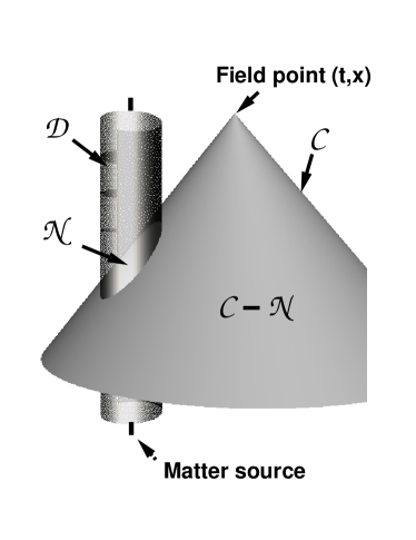
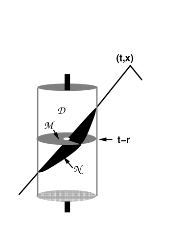
Figure 1: Past harmonic null cone $\cal C$ of the field point $(t,{\bf x})$ intersects the near zone $\cal D$ in the hypersurface $\cal N$.

Figure 2: Taylor expansion of retarded time dependence on $\cal N$ results in multipole moments integrated over the spatial hypersurface $\cal M$, corresponding to fixed retarded time $t-r$

The resolution of this problem involves taking literally the statement that the solution is a retarded integral, i.e. an integral over the entire past null cone of the field point.[opus] To be sure, that part of the integral that extends over the intersection $\cal N$ between the past null cone and the material source and the near zone is still approximated as usual by a slow-motion expansion involving spatial integrals over a constant-time hypersurface $\cal M$ of moments of the source, including the non-compact gravitational contributions, just as in the BDI framework (Fig. 2). But instead of cavalierly extending the spatial integrals to infinity as was implicit in the original EW framework, and risking undefined or divergent integrals, we terminate the integrals at the boundary of the near zone, chosen to be at a radius $\cal R$ given roughly by one wavelength of the gravitational radiation. For the integral over the rest of the past null cone exterior to the near zone (“radiation zone”), we neither make a slow-motion expansion nor continue to integrate over a spatial hypersurface, instead we use a coordinate transformation in the integral from the spatial coordinates $d^{3}x^{\prime}$ to quasi-null coordinates $du^{\prime}$, $d\theta^{\prime}$, $d\phi^{\prime}$, where

$$t-u^{\prime}=r^{\prime}+|{\bf x}-{\bf x}^{\prime}|\,,$$ (2)

to convert the integral into a convenient, easy-to-calculate form, that is manifestly convergent, subject only to reasonable assumptions about the past behavior of the source:

$$h_{{\cal C}-{\cal N}}^{\alpha\beta}(t,x)=4\int_{-\infty}^{u}du^{\prime}\int{{\tau^{\alpha\beta}(u^{\prime}+r^{\prime},{\bf x}^{\prime})}\over{t-u^{\prime}-{\bf n}^{\prime}\cdot{\bf x}}}[r^{\prime}(u^{\prime},\Omega^{\prime})]^{2}d^{2}\Omega^{\prime}\,.$$ (3)

This transformation was suggested by earlier work on a non-linear gravitational-wave phenomenon called the Christodoulou memory.[christo]  Not only are all integrations now explicitly finite and convergent, one can show that all contributions from the finite, near-zone spatial integrals that depend upon $\cal R$ are actually cancelled by corresponding terms from the radiation-zone integrals, valid for both positive and negative powers of $\cal R$ and for terms logarithmic in $\cal R$.[willpati]  Thus the procedure, as expected, has no dependence on the artificially chosen boundary radius $\cal R$ of the near-zone. In addition, the method can be carried to higher orders in a straightforward manner. The result is a manifestly finite, well-defined procedure for calculating gravitational radiation to high orders.

Thus, for field points in the far zone, the integral over the near zone takes the standard form of a multipole expansion, h_N^αβ(t, x) = 4 ∑_m=0^∞(-1)^m m! ∂^m ∂xk1…∂xkm ( 1 r M^αβk_1 …k_m(t-r) )  ,
M^αβk_1 …k_m(t-r) ≡∫_M τ^αβ (t-r,x^′)x^k_1^′ …x^k_m^′ d^3x^′ , where integrals are over the finite hypersurface $\cal M$. For field points in the near zone, the integral over the near zone can be expanded in the form of a sequence of “Poisson”-like potentials and superpotentials (and “superduper”-potentials) evaluated at a fixed time $t$:

$$h_{\cal N}^{\alpha\beta}(t,{\bf x})=4\sum_{m=0}^{\infty}{(-1)^{m}\over{m!}}{\partial^{m}\over{\partial t^{m}}}\int_{\cal M}\tau^{\alpha\beta}(t,x^{\prime})|{\bf x}-{\bf x}^{\prime}|^{m-1}d^{3}x^{\prime}\,.$$ (4)

In each case, the integrals must be combined with the corresponding integral over the rest of the past light cone, Eq. (3). Because of the aforementioned general proof, it is not necessary to keep any terms in these integrals that depend explicitly on the radius $\cal R$; this simplifies calculations considerably.

4 Equations of Motion to 3.5PN Order

We assume that the orbiting bodies are sufficiently small compared to their separation that tidal effects, or effects due to their finite size, can be ignored. For inspiralling compact binaries, this is believed to be a good approximation until the final few orbits. This amounts to replacing a perfect fluid stress-energy tensor,

$$T^{\mu\nu}=(\rho+p)u^{\mu}u^{\nu}+pg^{\mu\nu}\,,$$ (5)

with that of “point-masses”:

$$T^{\mu\nu}=\sum_{A}m_{A}\delta^{3}({\bf x}-{\bf x}_{A})u^{\mu}u^{\nu}/u^{0}\sqrt{-g}\,.$$ (6)

However, because of gravitational non-linearities, such a stress-energy tensor will lead to infinities at the location of each body, hence one must find a way to regularize in order to isolate the physically relevant terms. Blanchet et al. use a regularization procedure based on the Hadamard “partie fini”. Our approach, which is less formal, though probably equivalent, is to isolate those terms in any integral of fields over a body that neither vanish nor blow up as $D$, the size of the body, shrinks to zero. Terms that vanish as $D^{N}$ represent tidal and spin effects (and their relativistic generalizations), which we are ignoring. Terms that diverge as $D^{-N}$ are “self-energy” terms; we assume that these can be uniformly absorbed into renormalized masses for the bodies. It is important to stress that this is an assumption, whose validity has been checked in general only to 1PN order (no Nordtvedt effect in GR) and under restricted circumstances to 2PN order. The result is a well-defined procedure for keeping “finite, point-mass” terms.

With these assumptions, the equations of motion for each body take the form of a geodesic equation,

$$\rho^{*}{d^{2}x^{j}\over dt^{2}}+\rho^{*}\Gamma_{\mu\nu}^{j}v^{\mu}v^{\nu}-\rho^{*}\Gamma_{\mu\nu}^{0}v^{j}v^{\mu}v^{\nu}=0\,,$$ (7)

where $\rho^{*}=\rho u^{0}\sqrt{-g}\to\sum_{A}m_{A}\delta^{3}({\bf x}-{\bf x}_{A})$.

To obtain equations of motion valid through 3.5PN order, it is necessary to iterate the relaxed Einstein equation four times. Evaluating the resulting Poisson-like potentials for two fluid balls, integrating the equation of motion (7) over one of the bodies, and keeping only terms that are finite as the bodies shrink in size, one obtains equations of motion of the schematic form a_1^i &= -m_2 r2 [ n^i + O(ϵ) + O(ϵ^2) + O(ϵ^5/2) + O(ϵ^3) + O(ϵ^7/2) + …]  ,
a_2^i = m_1 r2 [ 1 ⇌2 ]  , where $r$ is the distance between the bodies and $n^{i}\equiv(x_{1}^{i}-x_{2}^{i})/r$. The expansion parameter $\epsilon$ is related to the orbital variables by $\epsilon\sim m/r\sim v^{2}$, $v$ is the relative velocity, and $m=m_{1}+m_{2}$ is the total mass ($G=c=1$).

We have evaluated all contributions to $h^{\mu\nu}$ formally through 3.5PN order in terms of Poisson-like potentials, and have calculated them explicitly for two compact bodies through 2.5PN order and at 3.5PN order. The formidable task of evaluating the contributions at 3PN order is in progress. At 2PN order, we obtain equations of motion in complete agreement with those of Damour and Deruelle (Eqs. (154) - (160) of Ref. damour300) and Blanchet et al. (Eq. (8.4) of Ref. lucfayeponsot).

The contributions at 2.5PN and 3.5PN order represent gravitional-radiation reaction and its post-Newtonian corrections. Iyer and Will [iyerwill] have shown that, assuming energy and angular momentum balance, the relative two-body equations of motion at 2.5PN order can be written in the form

$${\bf a}=-{8\over 5}\eta(m/r^{2})(m/r)\bigl{[}-(A_{2.5}+A_{3.5})\dot{r}{\bf n}+(B_{2.5}+B_{3.5}){\bf v}\bigr{]}\,,$$ (8)

where $\eta=m_{1}m_{2}/m^{2}$, $\dot{r}=dr/dt$, and A_2.5 &= (3+3β)v^2+(23 3 +2α-3β)m r - 5β˙r^2  ,
B_2.5 = (2+α)v^2 + (2-α)m r -3(1+α)˙r^2  , where $\alpha$ and $\beta$ are arbitrary, and reflect the effects of coordinate freedom on the equations of motion. The values $\alpha=4$, $\beta=5$ correspond to the so-called “Burke-Thorne” gauge, in which the radiation reaction is expressed solely as a quasi-Newtonian potential $\Phi_{RR}=-\frac{1}{5}M_{ij}^{(5)}(t)x^{i}x^{j}$, where $M_{ij}(t)$ is the traceless moment of inertia tensor of the system and the superscript $(5)$ denotes five time derivatives. This also corresponds to the gauge used by Blanchet [lucreaction]. Our 2.5PN equations of motion yield the values $\alpha=-1$, $\beta=0$, which corresponds to the gauge used by Damour and Deruelle (Eq. (161) of Ref. damour300).

At 3.5PN order, the expressions for $A_{3.5}$ and $B_{3.5}$ are A_3.5 &=a_1v^4+a_2v^2m/r+a_3v^2