A numeric solution for metric-affine gravity and Einstein’s gravitational theory with Proca matter

Abstract

A special case of metric-affine gauge theory of gravity (MAG) is equivalent to general relativity with Proca matter as source. We study in detail a corresponding numeric solution of the Reissner-Nordström type. It is static, spherically symmetric, and of electric type. In particular, this solution has no horizon, so it has a naked singularity as its origin.

1 Introduction

We will present a numeric solution of the Einstein-Proca theory with motivation that this theory is equivalent to a special case of the metric-affine gauge theory of gravity (MAG) [4]. This special case is the so-called triplet ansatz [6] in which, roughly, the lagrangian includes square terms of nonmetricity but also square terms of the derivative of nonmetricity (stemming from curvature squares). It is a special feature of this ansatz that the nonmetricity (as well as torsion) may be expressed by a 1-form, which, because of this type of lagrangian, represents a massive, propagating 1-form field, i.e. perfectly equivalent to a Proca field. Obukhov et al. [6] gave an exact proof of this equivalence.

The outline of this paper is rather straightforward: First, we briefly present the triplet ansatz and Obukhov’s theorem. Then we review the Einstein-Proca theory, set up the lagrangian, derive the field equations, and simplify them for a spherically symmetric ansatz. After addressing the problem of integration constants and dimensions we can perform the numerical integration. We also present a power series expansion of the solution around the origin. The most important features of our solution are summarized at the end.

MAG and the triplet ansatz

Given the curvature $R_{\alpha}{}^{\beta}$ and its 6+5 irreducible pieces ${}^{(I)}\hat{R}_{\alpha}{}^{\beta}$ and ${}^{(I)}\parbox{0.0pt}{~{}\raisebox{10.76385pt}{${}^{\circ}$}}R_{\alpha}{}^{\beta}$, the torsion $T_{\alpha}$ and its 3 irreducible pieces ${}^{(I)}T_{\alpha}$, and the nonmetricity $Q_{\alpha\beta}$ and its 4 irreducible pieces ${}^{(I)}Q_{\alpha\beta}$ (see [4] appendix B), we may write the general MAG lagrangian as

$$\mathcal{L}_{\rm MAG}=~{}\frac{1}{2\kappa}\Big{[} -~{}a_{0}R^{\alpha\beta}\wedge\eta_{\alpha\beta}-2\lambda\eta$$ à la Hilbert-Einstein

$$+~{}T^{\alpha}\wedge{}^{\star}(a_{I=1..3}{}^{(I)}T{}_{\alpha})$$ quadratic torsion

$$+~{}Q_{\alpha\beta}\wedge{}^{\star}(b_{I=1..4}{}^{(I)}Q^{\alpha\beta})$$ quadratic nonmetricity

$$+~{}b_{5}\,({}^{(3)}Q_{\alpha\gamma}\wedge\vartheta^{\alpha})\wedge{}^{\star}({}^{(4)}Q^{\beta\gamma}\wedge\vartheta_{\beta}) \vartheta^{\alpha}$$ quad. nonm. mixed with

$$+~{}2(c_{I=2..4}~{}^{(I)}Q_{\alpha\beta})\wedge\vartheta^{\alpha}\wedge{}^{\star}T^{\beta}\Big{]}$$ cross terms nonm./torsion

$$-~{}\frac{1}{2\varrho}R^{\alpha\beta}\wedge{}^{\star}\Big{[}(w_{I=1..6}{}^{(I)}\hat{R}_{\alpha\beta})+(z_{I=1..5}{}^{(I)}\parbox{0.0pt}{~{}\raisebox{10.76385pt}{${}^{\circ}$}}\!R_{\alpha\beta})$$ quadratic curvature

$$+w_{7}\,\vartheta_{\alpha}\wedge(e_{\gamma}\rfloor{}^{(5)}\hat{R}^{\gamma}{}_{\beta})+z_{6}\,\vartheta_{\gamma}\wedge(e_{\alpha}\rfloor{}^{(2)}\parbox{0.0pt}{~{}\raisebox{10.76385pt}{${}^{\circ}$}}\!R^{\gamma}{}_{\beta})$$

$$+z_{I=7..9}\,\vartheta_{\alpha}\wedge(e_{\gamma}\rfloor{}^{(I-4)}\parbox{0.0pt}{~{}\raisebox{10.76385pt}{${}^{\circ}$}}\!R^{\gamma}{}_{\beta})\Big{]}\;.\quad \Big{\}} \vartheta^{\alpha}$$ mixed with (1)

Here, we sum over the repeated index $I$. This lagrangian and the presently known solutions have been reviewed in [3]. We have the weak and strong coupling constants $1/\kappa$ and $1/\varrho$, the cosmological constant $\lambda$, and the 28 parameters $a_{I=0..3}$, $b_{I=1..5}$, $c_{I=2..4}$, $w_{I=1..7}$, and $z_{I=1..9}$. Note that the weak coupling constant has length dimension $[1/\kappa]=1/\ell^{2}$ because it multiplies to a torsion square, torsion being the field strength of translation generators with dimension $1/\ell$. The strong coupling constant, though, has no length dimension. The work presented here is only concerned with the so-called triplet ansatz, i.e. the special case

$$\varrho=1\;,\quad w_{I=1..7}=0\;,\quad z_{I=1..3}=z_{I=5..9}=0\;,\quad z_{4}\not=0\;.\quad$$ (2)

This means that we consider a general weak lagrangian (with weak coupling constant) but only a very restricted strong lagrangian (of curvature squares) allowing only for a square of the dilation curvature ${}^{(4)}\parbox{0.0pt}{~{}\raisebox{10.76385pt}{${}^{\circ}$}}R_{\alpha\beta}:=\frac{1}{n}\,g_{\alpha\beta}\,R_{\gamma}{}^{\gamma}$. Qualitatively, the lagrangian with these constraints may be displayed as

$$\mathcal{L}~{}~{}\sim~{}~{}\lambda~{}+~{}R~{}+~{}\big{(}T+Q\big{)}^{2}~{}+~{}\big{(}{}^{(4)}\parbox{0.0pt}{~{}\raisebox{10.76385pt}{${}^{\circ}$}}R\big{)}^{2}\;.$$ (3)

Here, $R$, $T$, and $Q$ denote just some terms linear in the curvature, torsion, and nonmetricity, respectively. On this qualitative level, the result of Obukhov et al. [6] is the following: Effectively, the curvature $R$ may be considered Riemannian, $T$ and $Q$ may be replaced by a 1-form $\phi$, i.e. $T+Q\sim\phi$, and ${}^{(4)}\parbox{0.0pt}{~{}\raisebox{10.76385pt}{${}^{\circ}$}}\!R$ is similar to $d\phi$. Hence, (3) reads generically

$$\mathcal{L}~{}~{}\sim~{}~{}\lambda~{}+~{}R_{\rm riem}~{}+~{}\phi^{2}~{}+~{}(d\phi)^{2}\;,$$ (4)

which describes an Einstein spacetime with a massive 1-form field $\phi$, i.e. a Proca field.

We will review the results of [6] in detail. First, one considers a special case of the MAG lagrangian (1) with constraint (2) by specifying the remaining parameters $\lambda$, $a_{I=0..3}$, $b_{I=1..5}$, $c_{I=2..4}$, and $z_{4}$. This choice is done in [6] eq (4.1) and turns out to effectively produce a purely Riemannian Hilbert-Einstein lagrangian, cf. [6] (4.6). This allows to introduce a new variable, the effective Riemannian curvature. Then, having investigated this special lagrangian, they generalize it again by adding a general lagrangian (restricted by (2)) to it, [6] (5.1-5.5). With the aid of the effective Riemannian curvature, the field equation FIRST (the variation with respect to the anholonomic coframe, see [4]) reads like an Einstein equation with an energy-momentum source that depends on torsion and nonmetricity, [6] (5.11). The field equation SECOND (the variation with respect to the linear connection) becomes a system of differential equations for torsion and nonmetricity alone. In the vacuum case, where the energy-momentum $\Sigma_{\alpha}$ and the hypermomentum $\Delta_{\alpha}{}^{\beta}$ of matter vanish, these differential equations (i.e. SECOND) reduce to

$${}^{(1)}T_{\alpha}=0\;,\quad^{(2)}T_{\alpha}=\frac{k_{2}}{3}\,\vartheta_{\alpha}\wedge\phi\;,\quad^{(3)}T_{\alpha}=0\;,\quad$$ cf. [6] (6.2,6.6+2.3,5.20)

$${}^{(1)}Q_{\alpha\beta}=0\;,\quad^{(2)}Q_{\alpha\beta}=0\;,\quad$$ cf. [6] (5.27,6.3)

$${}^{(3)}Q_{\alpha\beta}=\frac{4}{9}k_{1}\,\Big{(}\vartheta_{(\alpha}e_{\beta)}\rfloor\phi-\frac{1}{4}g_{\alpha\beta}\,\phi\Big{)}\;,\quad^{(4)}Q_{\alpha\beta}=k_{0}\,g_{\alpha\beta}\,\phi\;,\quad$$ cf. [6] (6.5+2.7,2.8)

$$d{}^{\star}d\phi+m^{2}\phi=0\;.\quad$$ cf. [6] (6.7) (5)

Here, the new 1-form $\phi$ determines the torsion and nonmetricity completely and needs to solve the Proca equation. The four constants $m$, $k_{0}$, $k_{1}$, and $k_{2}$ uniquely depend on the parameters of the MAG lagrangian via [6] (6.8, 6.4, 5.3-5.5). We summarize

$$k_{0} =4(a_{2}-2a_{0})(b_{3}+a_{0}/8)-3(c_{3}+a_{0})^{2}\;,\quad$$

$$k_{1} =9/2(a_{2}-2a_{0})(b_{5}-a_{0})-9(c_{3}+a_{0})(c_{4}+a_{0})\;,\quad$$

$$k_{2} =12(b_{3}+a_{0}/8)(c_{4}+a_{0})-9/2(b_{5}-a_{0})(c_{3}+a_{0})\;,\quad$$

$$m^{2} =\frac{1}{z_{4}\kappa}\left(-4b_{4}+\frac{3}{2}\,a_{0}+\frac{k_{1}}{2k_{0}}\,(b_{5}-a_{0})+\frac{k_{2}}{k_{0}}\,(c_{4}+a_{0})\right)\;.\quad$$ (6)

Obviously, these parameters depend only on $a_{0}$, $a_{2}$, $b_{3}$, $b_{4}$, $b_{5}$, $c_{3}$, $c_{4}$, and $z_{4}$. With (5) and (6) we can express the energy-momentum source of torsion and nonmetricity in the effective Einstein equation in terms of $\phi$ [6] (7.3, 7.5). This energy-momentum is exactly the energy-momentum of the Proca 1-form $\phi$. Hence, we finally found that the MAG lagrangian (1), restricted by (2), together with its field equations, is effectively equivalent to an Einstein-Proca lagrangian as suggested in (4). The parameter $m$ given in (6) has the meaning of the mass parameter of the Proca 1-form $\phi$. If $m$ vanishes, the initial MAG theory is equivalent to the Einstein-Maxwell theory. In general, $m=0$ is equivalent to

$$0 =32\,{b_{4}}\,{a_{2}}\,{b_{3}}-12\,{a_{0}}\,{a_{2}}\,{b_{3}}-64\,{b_{4}}\,{a_{0}}\,{b_{3}}-24\,{b_{3}}\,{c_{4}}^{2}-48\,{b_{3}}\,{c_{4}}\,{a_{0}}-32\,{b_{4}}\,{a_{0}}^{2}-24\,{b_{4}}\,{c_{3}}^{2}$$

$$+9\,{a_{2}}\,{b_{5}}\,{a_{0}}-6\,{a_{2}}\,{a_{0}}^{2}+9\,{a_{0}}\,{c_{3}}^{2}-48\,{b_{4}}\,{c_{3}}\,{a_{0}}+4\,{b_{4}}\,{a_{2}}\,{a_{0}}-24\,{a_{0}}^{2}\,{c_{4}}+9\,{a_{0}}\,{b_{5}}^{2}$$

$$-\frac{9}{2}\,{a_{2}}\,{b_{5}}^{2}-3\,{a_{0}}\,{c_{4}}^{2}+18\,{c_{3}}\,{c_{4}}\,{b_{5}}-18\,{c_{3}}\,{c_{4}}\,{a_{0}}+18\,{c_{3}}\,{a_{0}}\,{b_{5}}+18\,{a_{0}}\,{c_{4}}\,{b_{5}}\;.\quad$$ (7)

This equation generalizes [7] (4.2) for $b_{5}\not=0$. Thus, the exact solution found in [7] with $m=0$ corresponds to an exact solution of an Einstein-Maxwell system. Here, we want to present a solution for $m\not=0$.

2 The Einstein-Proca theory

Motivated by the previous section we now concentrate on the Proca lagrangian $\mathcal{L}_{P}$ of a massive 1-form $\phi$:

$$\mathcal{L}_{P} =-\frac{1}{2}\,d\phi\wedge{}^{\star}d\phi+\frac{1}{2}\,m^{2}\phi\wedge{}^{\star}\phi\;.\quad$$ (8)

First, we shortly discuss the dimension of $m$. We know that the Hodge-dual of a $p$-form is an $(n\!-\!p)$-form. Hence, whenever the Hodge-dual applies on a $p$-form, it has the dimension $[\,{}^{\star}\,]=\ell^{n-2p}$. It follows that $[d\phi\wedge{}^{\star}d\phi]=[\phi]^{2}$, and $\phi\wedge{}^{\star}\phi=\ell^{2}[\phi]^{2}$. To be able to consistently add these terms in the lagrangian the dimension of the mass parameter needs to be $[m]=1/\ell$.

It is straightforward to calculate the Proca field equation and the canonical energy-momentum of this lagrangian with the Noether-Lagrange machinery presented in [4]. The variations yield:

$$\frac{\delta\mathcal{L}_{P}}{\delta\phi} =d\frac{\partial\mathcal{L}_{P}}{\partial(d\phi)}+\frac{\partial\mathcal{L}_{P}}{\partial\phi}=-d{}^{\star}d\phi+m^{2}\,{}^{\star}\phi\;,\quad$$ (9)

$$\frac{\delta\mathcal{L}_{P}}{\delta\vartheta^{\alpha}} =:\Sigma_{\alpha}=e_{\alpha}\rfloor\mathcal{L}_{P}-(e_{\alpha}\rfloor d\phi)\frac{\partial\mathcal{L}_{P}}{\partial d\phi}-(e_{\alpha}\rfloor\phi)\frac{\partial\mathcal{L}_{P}}{\partial\phi}$$

$$=\frac{1}{2}\left[-(e_{\alpha}\rfloor d\phi)\wedge{}^{\star}d\phi-d\phi\wedge(e_{\alpha}\rfloor{}^{\star}d\phi)+m^{2}(e_{\alpha}\rfloor\phi)\wedge{}^{\star}\phi-m^{2}\phi\wedge(e_{\alpha}\rfloor{}^{\star}\phi)\right]$$

$$\quad+(e_{\alpha}\rfloor d\phi)\wedge{}^{\star}d\phi-m^{2}(e_{\alpha}\rfloor\phi)\wedge{}^{\star}\phi$$

$$=\frac{1}{2}\left[(e_{\alpha}\rfloor d\phi)\wedge{}^{\star}d\phi-d\phi\wedge(e_{\alpha}\rfloor{}^{\star}d\phi)-m^{2}\left[(e_{\alpha}\rfloor\phi)\wedge{}^{\star}\phi+\phi\wedge(e_{\alpha}\rfloor{}^{\star}\phi)\right]\right]\;.\quad$$ (10)

Coupled with a Riemannian background, i.e. considering a lagrangian
$\mathcal{L}=\mathcal{L}_{P}+\mathcal{L}_{\rm Hilbert-Einstein}$, we end up with the field equations

$$0=-d{}^{\star}d\phi+m^{2}\,{}^{\star}\phi\;,\quad \mbox{Proca equation}\;,\quad$$ (11)

$$0=G_{\alpha}-\kappa\Sigma_{\alpha}=:X_{\alpha}\;,\quad \mbox{Einstein equation}\;.\quad$$ (12)

For completeness we also display the contracted Bianchi identities

$$0=d\Sigma^{\alpha}+\Gamma_{\beta}{}^{\alpha}\wedge\Sigma^{\beta}\;.$$ (13)

Also Obukhov and Vlachynsky [5] considered this system and indeed found the same solution we will find. Unfortunately, they did not publish their results until recently such that the author did not know about their efforts for a long time. However, the integration and the results are presented here in much more detail. Before we concentrate on a solution of this system, we consider two modified versions of the problem.

2.1 A Proca field on flat spacetime background

If we consider the lagrangian (8) on flat, i.e. Minkowskian background we find two simple solutions. The first we find by an ansatz in analogy to the static electric monopole field $A_{\rm el}=q/r\,dt$: We suppose $\phi$ to be a static, spherically symmetric, and time-like 1-form

$$\phi=\frac{u_{\rm el}(r)}{r}\,dt\;,$$ (14)

where $t$ denotes the time coordinate and $r$ the radius in spherical coordinates. With this ansatz, the Proca equation (11) becomes

$$0=\frac{1}{r}\,(-u_{\rm el}^{\prime\prime}+m^{2}\,u_{\rm el})$$ (15)

and can be solved by the well known Yukawa potential

$$\frac{u_{\rm el}(r)}{r}=\frac{q}{r}\,\exp(-mr)\;.$$ (16)

The parameter $q$ is called Proca charge. A second solution we find by considering an ansatz in analogy to the static magnetic monopole field $A_{\rm mag}=p\,(1-\cos\theta)\,d\varphi$: We set

$$\phi=u_{\rm mag}(r)\,(1-\cos\theta)\,d\varphi\;.$$ (17)

The field equations (11) becomes

$$0=\frac{1}{r\,\sin\theta}\,(1-\cos\theta)(-u_{\rm mag}^{\prime\prime}+m^{2}\,u_{\rm mag})$$ (18)

which is, of course, also solved by $u_{\rm mag}=p\,\exp(-mr)$, where $p$ might be called magnetic Proca charge.

2.2 A Proca vector field

Here we want to clarify that there is a difference between an ansatz of $\phi$ as a 1-form and as a vector. Consider the analogy of the lagrangian (8) for a vector-valued 0-form $\phi_{\alpha}$:

$$\mathcal{L}_{P} =-D\phi^{\alpha}\wedge{}^{\star}D\phi_{\alpha}\;+\;m^{2}\phi^{\alpha}\wedge{}^{\star}\phi_{\alpha}\;,\quad$$ (19)

$$\frac{\delta\mathcal{L}_{P}}{\delta\phi^{\alpha}} =-D\frac{\partial\mathcal{L}_{P}}{\partial(D\phi^{\alpha})}+\frac{\partial\mathcal{L}_{P}}{\partial\phi^{\alpha}}=+2\,D{}^{\star}D\phi_{\alpha}+2\,m^{2}\,{}^{\star}\phi_{\alpha}\;,\quad$$ (20)

$$\frac{\delta\mathcal{L}_{P}}{\delta\vartheta^{\alpha}} =:\Sigma_{\alpha}=e_{\alpha}\rfloor\mathcal{L}_{P}-(e_{\alpha}\rfloor D\phi^{\beta})\frac{\partial\mathcal{L}_{P}}{\partial D\phi^{\beta}}-(e_{\alpha}\rfloor\phi^{\beta})\frac{\partial\mathcal{L}_{P}}{\partial\phi^{\beta}}$$

$$=-(e_{\alpha}\rfloor D\phi^{\beta})\wedge{}^{\star}D\phi_{\beta}+D\phi^{\beta}\wedge(e_{\alpha}\rfloor{}^{\star}D\phi_{\beta})+m^{2}(e_{\alpha}\rfloor\phi^{\beta})\wedge{}^{\star}\phi_{\beta}+m^{2}\phi^{\beta}\wedge(e_{\alpha}\rfloor{}^{\star}\phi_{\beta})$$

$$+2(e_{\alpha}\rfloor D\phi^{\beta})\wedge{}^{\star}D\phi_{\beta}-2m^{2}(e_{\alpha}\rfloor\phi^{\beta})\wedge{}^{\star}\phi_{\beta}$$

$$=(e_{\alpha}\rfloor D\phi^{\beta})\wedge{}^{\star}D\phi_{\beta}+D\phi^{\beta}\wedge(e_{\alpha}\rfloor{}^{\star}D\phi_{\beta})-m^{2}\left[(e_{\alpha}\rfloor\phi^{\beta})\wedge{}^{\star}\phi_{\beta}-\phi^{\beta}\wedge(e_{\alpha}\rfloor{}^{\star}\phi_{\beta})\right]$$

$$=(e_{\alpha}\rfloor D\phi^{\beta})\wedge{}^{\star}D\phi_{\beta}+D\phi^{\beta}\wedge(e_{\alpha}\rfloor{}^{\star}D\phi_{\beta})+m^{2}\phi^{\beta}\wedge(e_{\alpha}\rfloor{}^{\star}\phi_{\beta})\;.\quad$$ (21)

Note that we introduced the covariant derivative $D=d+\Gamma^{\{\}}$ with the Levi-Civita connection $\Gamma^{\{\}}$. In flat space, say, we find that the signs in (20) and (11) do not agree. Also, the energy-momentum (21) is very different from (10). From the introduction it is clear that we are interested in a Proca 1-form and not in a Proca vector field.

3 An solution with electric type Proca field

Motivated by the Yukawa solution $\phi=\frac{q\,\exp(-mr)}{r}\,dt$ of the flat Proca equation and the analogy to the electric monopole, we make the ansatz that $\phi$ is a spherically symmetric, static, and time-like 1-form:

$$\phi=\frac{u(r)}{r}dt\;.$$ (22)

The general spherically symmetric ansatz for the coframe (i.e. implicitly for the metric) reads

$$\vartheta^{\hat{0}}=f\,dt\;,\quad\vartheta^{\hat{1}}=\frac{g}{f}\,dr\;,\quad\vartheta^{\hat{2}}=r\,d\theta\;,\quad\vartheta^{\hat{3}}=r\sin\theta\,d\varphi\;,\quad f=f(r)\;,\quad g=g(r)\;.\quad$$ (23)

The meaning of the function $g$ is illustrated by the relation $\eta=g\,\eta_{\rm flat}$ for the volume element $\eta={}^{\star}1$. Writing the Proca field as $\phi=\Phi(r)\,dt$, with $\Phi(r):=u(r)/r$, the energy-momentum (10) of this ansatz turns out to be

$$\vartheta^{\hat{0}}\wedge\Sigma^{\hat{0}} =\frac{\eta}{2}\left[-(\Phi^{\prime}/g)^{2}-m^{2}\Phi^{2}/f^{2}\right]\;,\quad$$

$$\vartheta^{\hat{1}}\wedge\Sigma^{\hat{1}} =\frac{\eta}{2}\left[~{}~{}\,(\Phi^{\prime}/g)^{2}-m^{2}\Phi^{2}/f^{2}\right]\;,\quad$$

$$\vartheta^{\hat{2}}\wedge\Sigma^{\hat{2}} =\frac{\eta}{2}\left[-(\Phi^{\prime}/g)^{2}-m^{2}\Phi^{2}/f^{2}\right]\;,\quad$$

$$\vartheta^{\hat{3}}\wedge\Sigma^{\hat{3}} =\frac{\eta}{2}\left[-(\Phi^{\prime}/g)^{2}-m^{2}\Phi^{2}/f^{2}\right]\;,\quad$$

$$\vartheta^{\mu}\wedge\Sigma^{\nu} =0\quad\mbox{for $\mu\not=\nu$}\;,\quad$$

$${}^{\star}(\vartheta^{\alpha}\wedge\Sigma_{\alpha}) =-\frac{m^{2}\Phi^{2}}{f^{2}}\;,\quad$$

$${}^{\star}(\Sigma_{\alpha}\wedge{}^{\star}\Sigma^{\alpha}) =\Big{(}\frac{\Phi^{\prime}}{g}\Big{)}^{4}+\Big{(}\frac{\Phi^{\prime}m\Phi}{fg}\Big{)}^{2}+\Big{(}\frac{m\Phi}{f}\Big{)}^{4}\;.\quad$$ (24)

Recall that ${}^{\star}(\vartheta^{\mu}\wedge\Sigma^{\nu})=:T^{\mu\nu}$ represent the components of the ordinary 2nd rank energy-momentum tensor. The non-vanishing components of equations (11), (12), and (13) read in simplified form

$$\text{P}_{0}: ~{}~{}0=f^{2}g^{\prime}(u-ru^{\prime})+gr(f^{2}u^{\prime\prime}-g^{2}m^{2}u)$$

$$\text{P}_{1}: ~{}~{}0=g\dot{u}+\dot{g}(ru^{\prime}-u)$$

$$\text{E}_{00}: ~{}~{}0=-\kappa\big{[}(u-ru^{\prime})^{2}+m^{2}r^{2}u^{2}g^{2}/f^{2}\big{]}+2r^{2}(f^{2}-g^{2})+4ff^{\prime}r^{3}-4f^{2}r^{3}g^{\prime}/g$$

$$\text{E}_{11}: ~{}~{}0=-\kappa\big{[}(u-ru^{\prime})^{2}-m^{2}r^{2}u^{2}g^{2}/f^{2}\big{]}+2r^{2}(f^{2}-g^{2})+4ff^{\prime}r^{3}$$

$$\text{E}_{01}: ~{}~{}0=f\dot{g}-g\dot{f}$$

$$\text{E}_{22}: ~{}~{}0=-\kappa gf^{4}\big{[}(u-ru^{\prime})^{2}+m^{2}r^{2}u^{2}g^{2}/f^{2}\big{]}+2g^{2}r^{4}f(f\ddot{g}-g\ddot{f})-6\dot{f}(f\dot{g}-g\dot{f})$$

$$~{}~{}~{}~{}~{}+2f^{4}r^{4}f^{\prime}(fg^{\prime}-gf^{\prime})-2f^{5}f^{\prime\prime}gr^{4}+2f^{5}r^{3}(fg^{\prime}-2gf^{\prime})$$

$$\text{B}_{0}: ~{}~{}0=f^{3}(ru^{\prime}-u)\big{[}g\dot{u}+\dot{g}(ru^{\prime}-u)\big{]}-g^{2}m^{2}r^{2}u\big{[}g(f\dot{u}-u\dot{f})+u(f\dot{g}-g\dot{f})\big{]}$$

$$\text{B}_{1}: ~{}~{}0=f^{2}g^{\prime}(u-ru^{\prime})+gr(f^{2}u^{\prime\prime}-g^{2}m^{2}u)$$ (25)

Here, P, E, and B refer to the Proca, Einstein, and contracted Bianchi equations and indices denote the respective components. These equations also include, for later purposes, the case of time dependent functions $u$, $f$, and $g$. Here, we neglect this time dependence and thus discard all time derivatives. We see that $\text{B}_{1}$ is equivalent to $\text{P}_{0}$ and that $\text{E}_{11}-\text{E}_{00}$ simplifies the Einstein equations a lot. We end up with the following ordinary differential equations system of second order in $u$ and first order in $f$ and $g$:

$$\text{P}_{0}: ~{}~{}0=f^{2}g^{\prime}(u-ru^{\prime})+gr(f^{2}u^{\prime\prime}-g^{2}m^{2}u)\;,$$ (26)

$$\text{E}_{11}: ~{}~{}0=-\kappa\big{[}(u-ru^{\prime})^{2}-m^{2}r^{2}u^{2}g^{2}/f^{2}\big{]}+2r^{2}(f^{2}-g^{2})+4ff^{\prime}r^{3}\;,$$ (27)

$$\text{E}_{11}-\text{E}_{00}: ~{}~{}0=\kappa m^{2}u^{2}g^{3}+4f^{4}rg^{\prime}\;.$$ (28)

These equations are equivalent to [5] eqs (3.5, 3.9, 3.10) found by Obukhov and Vlachynsky. We did most of the calculations with the aid of the computer algebra systems Reduce and Maple. The respective files can be found at www.thp.uni-koeln/~mt/work/1999diplom/.

3.1 Preparing the numerical integration

First we briefly discuss the dimensions of the system. We know the dimensions of the radius, the gravitational coupling constant, and the Proca mass, $[r]=\ell$, $[\kappa]=\ell^{2}$, $[m]=1/\ell$, respectively. Hence, we get rid of all dimensions by rescaling the radius variable $r\to r/\sqrt{\kappa}$ and the mass parameter $m\to\sqrt{\kappa}\,m$. In practice, i.e. when investigating the equation system with computer algebra, we simply put $\kappa\equiv 1$, which is equivalent to the rescaling but saves us from introducing new variables. Also, we can eliminate the mass parameter $m$ from (26-28) by the substitution $r\to m\,r$, $f\to f/m$, and $g\to g/m$. Instead, again, we equivalently fix $m=1$ in the following without loosing generality.

We now concentrate on the dimensionless ordinary differential equation system (26-28). Parameter $m$ is fixed and obviously not an integration constant. The equation system is of first order in $f$ and $g$, and of second order in $u$. It is easy to reduce it to an ordinary first order differential equation system by substituting $u^{\prime}\to v$, $u^{\prime\prime}\to v^{\prime}$ and by adding a fourth equation $v=u^{\prime}$ to the system. Hence, a general integration of this system leads to four integration constants. In the case of a numerical approach, these constant are the initial values for $f$, $g$, $u$, and $u^{\prime}$ at the starting point of integration. Here, we consider only two starting points $r_{0}\ll 1$ and $r_{\infty}\gg 1$ for integrations from zero and infinity. We denote the set of integration constants by $(f_{0},g_{0},u_{0},u^{\prime}_{0})$ in one case and by $(f_{\infty},g_{\infty},u_{\infty},u^{\prime}_{\infty})$ in the other. The discussion above suggests that we will find a 4-parameter set of solutions. But this is misleading. In principle it is possible to start integration with four arbitrary parameters at some point $\tilde{r}\in\mathrm{I\!R}$. But then, in general, one will find a solution of the equations (26-28) only in a neighborhood of $\tilde{r}$. More precisely, the convergence for $r\to 0$ and $r\to\infty$ are 2 constraints and thus we expect only a 2-parameter set of suitable integration constants.

First we discuss the limit $r\to 0$. We presume that $g$, $u$, and $u^{\prime}$ are finite at zero and that $f$ diverges as $1/r$. This can be motivated by the fact that such an ansatz solves the system of equations (26-28) as we will show shortly, or by the arguments that $g$ needs to be finite because of the volume element, $u$ and $u^{\prime}$ should be finite because of the energy, and $f$ should behave as $1/r$ because of the analogy to the Reissner-Nordström solution. Later, also our numerical integrations confirm this assumption. To investigate the limit $r\to 0$ we therefore insert the expansion

$$u =u_{1}+u_{2}\,r+u_{3}\,r^{2}+..\;,\quad$$

$$g =g_{1}+g_{2}\,r+g_{3}\,r^{2}+..\;,\quad$$

$$f =f_{1}/r+f_{2}+f_{3}\,r+..$$ (29)

into the system (26-28). Collecting the coefficients of 0-th order in $r$ in each of the three equations we find respectively

$$0 =f_{1}\,g_{2}\,u_{1}\;,$$

$$0 =f_{1}^{4}\,g_{1}-\frac{1}{2}h_{1}^{2}\,g_{1}\,u_{1}^{2}\;,$$

$$0 =h_{1}^{4}\,g_{2}\;.$$ (30)

These equations are solved by $g_{2}=0$ and $f_{1}=u_{1}/\sqrt{2}$. This means that, for $r\to 0$, we find the following approximate solution of the equation system (26-28):

$$f_{0} =\frac{q}{\sqrt{2}r_{0}}\;,\quad$$

$$g_{0} =c\;,\quad$$

$$u_{0} =q\;,\quad$$

$$u^{\prime}_{0} =b\;.\quad$$ (31)

Hence, for an integration from zero we are left three parameters $(q,b,c)$. Our results in section 3.4 will show that such solutions with arbitrary $(q,b,c)$ diverge at some finite radius. Only a fine tuning of one of the parameters (we tuned $c$) makes the solution converging at infinity. Hence, regarding only converging, global solutions, we are left with a 2-parameter set of solutions parameterized by $(q,b)$.

For the limit $r_{\infty}$ it is natural to require the metric function to tend to the Schwarzschild solution with the new mass parameter $M$ that represents the total gravitating mass. Also, the Proca field should tend to the vacuum solution of the Proca equation, i.e. the Yukawa potential specified by the new Proca charge parameter $Q$. In detail we would expect

$$f_{\infty} =\sqrt{1-\frac{2M}{r_{\infty}}}\;,\quad$$

$$g_{\infty} =1\;,\quad$$

$$u_{\infty} =Q\,\exp(-mr_{\infty})\;,\quad$$

$$u^{\prime}_{\infty} =-mQ\,\exp(-mr_{\infty})\;.\quad$$ (32)

This gives a 2-parameter set of solutions parameterized by $(M,Q)$. Since we sill find (numerically) that all of these solutions converge for $r\to 0$ we conclude that this set of solutions contains all global solutions.

A power series expansion

There exists a simple scheme to determine all coefficients in the expansion (29): Inserting the expansion and considering the coefficients of $i$-th order ($i\geq 2$) in $r$ in each of the three equations (26-28), one can solve for $u_{i+2}$, $g_{i+2}$, and $f_{i+1}$ in terms of $u_{j+2}$, $g_{j+2}$, and $f_{j+1}$ with $j<i$. This iteration is very easily implemented in Maple and we display here the result after considering the equations up to 4-th order:

$$u(r)= q+b\,r-\frac{1}{10}\,\frac{c^{2}\,b}{q^{2}}\,r^{5}\;,$$ (33)

$$g(r)= c+{\frac{1}{2}}\,\frac{c^{3}}{q^{2}}\,r^{4}+\frac{4}{5}\,\frac{c^{3}\,b}{q^{3}}\,r^{5}\;,$$ (34)

$$f(r)= \frac{1}{\sqrt{2}}\,\frac{q}{r}+\frac{1}{\sqrt{2}}\,\frac{c^{2}}{q}\,r+\frac{1}{6\sqrt{2}}\,\frac{2\,q^{2}\,c^{2}-3\,c^{4}}{q^{3}}\,r^{3}\;.$$ (35)

The problems is that an insertion of the power expansion (29) into the equation system exceeds the computer’s memory resources very fast. Being limited in this way, we could not observe an appropriate convergence behavior for large $r$.

3.2 Integration from infinity for various $M$ and $Q$

We perform the numerical integration with the standard Runge-Kutta method provided by the computer algebra system Maple. (In detail: We used the rkf45 method with 15 digits, absolute (abserr) and relative (relerr) errors $10^{-13}$, and unlimited number of function evaluations (maxfun).) Such an integration takes only about 10 seconds. You can find all calculations in the Maple-file given.

Figure 1: Typical solution: Integration of (26-28) for $m=M=Q=1$ from $r_{\infty}=60$, with integration constants (32) performed by Maple. We see the metric functions $f$, $g$, and $h:=r\,f$, the Proca function $u$ and $u^{\prime}$, and the energy-momentum trace $t$ and its integral $s$ (divided by 100).

Figure 1 represents a typical solution for an integration from infinity ($r_{\infty}=60$, which is far enough from the Schwarzschild radius $r_{\rm S}(M)$). The gravitating mass $M$ and the Proca charge $Q$ are of the same order as $m=1$. We see the metric functions $f$ and $g$. To get a better impression of the behavior of $f$ for $r\to 0$ we add a plot of $h:=rf$. The asymptote of $h$ for $r\to\infty$ ($h\sim r\sqrt{1-2M/r}\sim r-M$) crosses the r-axis at $r=M$. The Proca function $u=\Phi/r$ exhibits a nicely localized density. Its derivative $-u^{\prime}$ is less instructive. Also the energy-momentum trace of the Proca field

$$t:=-{}^{\star}(\vartheta^{\alpha}\wedge\Sigma_{\alpha})=m^{2}\Phi^{2}/f^{2}=m^{2}u^{2}/h^{2}$$ (36)

(see (24)) is quite localized. We also display its spatial integral

$$s(r):=4\pi\int_{r}^{\infty}r^{2}g(r)t(r)\,dr\quad\text{satisfying}\quad\int_{\rm spatial}\vartheta^{\alpha}\wedge\Sigma_{\alpha}=-s(0)\,dt\;.$$ (37)

Figure 2: Integration from $r_{\infty}$. The metric functions $h=r\,f$ and $f^{2}$ are displayed for various $M$ and $Q$. For a better comparison, we plot the Reissner-Nordström solution in the right bottom.

Next we vary $M$ and $Q$. Figure 2 displays the metric functions $h=rf$ and $f^{2}$. The most interesting point of these plots is the following. For the Schwarzschild solution, $f^{2}$ becomes negative within the horizon and vanishes at the horizon. Looking at the energy-momentum of the Proca field $t:=m^{2}\Phi^{2}/f^{2}$, we can already follow that in our case $f^{2}$ may neither vanish nor be negative, as long as $\Phi$ is finite. Hence, a Proca solution with finite $\Phi$ may not have a horizon. For a better comparison, the lower two plots in figure 2 display $f^{2}$ for our Proca system (left plot) and the square metric function of the Reissner-Nordström solution (right plot) for varying Proca charge and electric charge, respectively. The Reissner-Nordström solution lacks a horizon as long as we choose the electric charge larger then $2M$, i.e. the over extreme case. For smaller charges the Reissner-Nordström solution has a horizon and the square metric function becomes negative. For our Proca system the behavior is similar for large $Q$. For smaller $Q$ though, $f^{2}$ approaches zero but never becomes negative. The important result that our solution has no horizon is consistent with the analysis of Ayón-Beato et al. [1]. They proved that a static Einstein-Proca solution may not have a horizon by considering a spatial integral of the Proca equation. They called this a no-hair theorem for static black holes in the Einstein-Proca theory – or in the equivalent triplet ansatz of MAG. The lack of a horizon also means that our solutions have no continuous limit for $m\to 0$ ($m=0$ means a Reissner-Nordström solution) or $Q\to 0$ ($Q=0$ generates a Schwarzschild solution)!

Figure 3: Integration from $r_{\infty}$. The metric function $g$ and the Proca function $u$ are displayed for various $M$ and $Q$.

In figure 3 we plot the metric function $g$ and the Proca function $u$. As we vary $M$, the metric function $g$ seems to distinguish inside and outside regions. Inside, $g$ takes some constant value within $[0,1]$ decreasing with increasing $M$. Outside, $g$ equals 1. As we vary $Q$, we find that larger values for $Q$ smear this boundary between inside and outside. Looking at the Proca function $u$, as we vary $M$, we find that the Proca field becomes perceptibly non-vanishing exactly within the same boundary $g$ exhibits. Very interesting is the curve for $M=0.6$ and $Q=0.05$ in the right plots. The Proca field vanishes as $r\to 0$ and its derivative $u^{\prime}$ becomes positive. The metric function $g$ approaches zero within the boundary instead of continuously approaching a finite $g(0)$ as it does for larger $Q$. This behavior is different indeed and belongs to region II as we will explain in the following section.

3.3 Comparing internal and external parameters

After the explicit presentation of the spherically symmetric solution of the Einstein-Proca system, we want to examine how the external parameters $M$ and $Q$ are correlated to the internal parameters $q$, $b$, and $c$. Both, $Q$ and $q$, are in analogy to the Proca charge – but with respect to different limits $r\to\infty$ and $r\to 0$, respectively. How are they related? The computational power of Maple allows to integrate the system for a quite large array of values of $M$ and $Q$. For this array we calculated the values of the internal parameters $q=u(0)$, $b=u^{\prime}(0)$, and $c=g(0)$ and display them in figure 4.

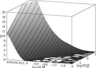
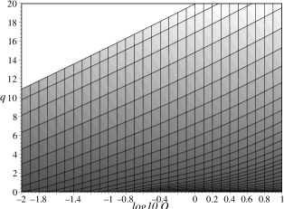
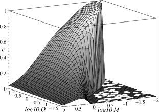
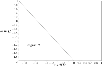
Figure 4: The field configuration $q=u(0)$, $b=u^{\prime}(0)$, and $c=g(0)$ at zero is displayed for an array $[-2<\log_{10}M<1,-2<\log_{10}Q<1]$ of different values for the external parameters $M$ and $Q$.

The first two of these plots display the internal Proca charge $q$. One can see that for any $M$, the internal $q$ depends approximately linear on $\log_{10}Q$:

$$q=\alpha\,\log_{10}Q+\beta\;,\qquad\text{where roughly }3<\alpha<4.5\;.$$ (38)

In the white regions of the left plot, the numerical integration could not reach the requested accuracy of $10^{-13}$ (relative and absolute error). The next two plots in figure 4 show $b$ and $c$. The noisy peaks in the plot of $b$ are at the very edge to regions where the integration could not reach the requested accuracy. However, we observe a smooth transition to positive values of $b$. This region II belongs to small values of $M$ and $Q$ as the diagram at the bottom illustrates. Also the plot of $c$ clearly demonstrates this edge to region II but at the same time exhibits the smooth transition to this region for smaller Q. We cannot completely exclude that this behavior is an artifact of the numerical integration. It is interesting that this region represents the limit $Q\to 0$ which, as we discussed above, cannot be continuous.

3.4 Solutions with fixed internal Proca charge

Figure 5: The integration from zero for arbitrary constants $q$, $b$, and $c$: If $c$ is too large (left plot) the Proca function $u$ diverges to $+\infty$, whereas if $c$ is too small (right plot) $u$ diverges to $-\infty$. Note the small difference of 0.0012 between the two values of $c$.

As we already mentioned, the integration from zero is quite costly. If we start integration with the constants (31) with arbitrary $q$, $b$, and $c$, the solution diverges at some finite radius. Figure 5 displays the two possible divergences: the Proca function $u$ either diverges to $+\infty$, if $c$ is large, or to $-\infty$, if $c$ is small. Only a fine tuning of $c$ allows to find a global solution by an integration from zero. Of course, these integrations exhibit the same solution as an integration from $\infty$. Since this procedure is very time expensive, we had to find another way to produce solutions with fixed internal Proca charge by using the relation (38) between $q$ and $Q$. We fixed $q$ by tuning $Q$ for given $M$. This may be done very quickly because if we have found one solution with arbitrary $q$, relation (38) tells us of how to approximately choose $Q$ for a given value of $q$. Thereby we need only about five steps to fix $q$ on a given value up to an accuracy of $10^{-5}$. Figure 6 shows how $Q$ has to be chosen for different $M$ in order to fix $q=1$. Figure 7 displays the solutions for fixed $q=1$ and different $M$. The plot of $h$ nicely demonstrates the necessary relation $h(0)=q/\sqrt{2}$ we found in (31). The plot of $f^{2}$, again, demonstrates that our solutions do not have a horizon. Instead, $f^{2}$ approaches zero but never becomes negative. Finally, the plots of $g$ and $u$ exhibit the localization of our Proca particle within a finite radius.

Figure 6: How to choose $Q$ for given $M$ in order to fix $q=1$.

Figure 7: The metric functions $h=r\,f$, $f^{2}$, and $g$ and the Proca function $u$ for fixed internal Proca charge $q=1$.

4 Other approaches

Failure of the magnetic type ansatz

In section 2.1 we found a solution $\phi=p\,\exp(-mr)\,(1-\cos\theta)\,d\varphi$ for the flat Proca equation (11). However, with the general spherically symmetric ansatz (23) for the coframe, we find the 12-component of the Einstein equation:

$$\vartheta^{1}\wedge X^{2}=\frac{f\kappa uu^{\prime}(\cos\theta-1)}{gr^{3}\sin\theta}\ \eta$$ (39)

which has only trivial solutions. Hence, there exists no magnetic analogue to the previous solution!

Rosen’s ansatz

In this section we have a glance on the ansatz of Rosen [8]. He considered the lagrangian (8) of a Proca 1-form together with the ansatz

$$\phi=w_{0}(r){\rm e}^{-i\omega t}\,dt+w_{1}(r){\rm e}^{-i\omega t}\,dr\;.\quad$$ (40)

With (40) and the spherically symmetric coframe (23), the Proca equation (11) reads

$$0 =\vartheta^{0}\wedge\vartheta^{2}\wedge\vartheta^{3}~{}\frac{{\rm e}^{-i\omega t}}{fg}~{}\Big{[}w_{1}(f^{2}m^{2}-\omega^{2})-i\omega w_{0}^{\prime}\Big{]}$$

$$-\vartheta^{1}\wedge\vartheta^{2}\wedge\vartheta^{3}~{}\frac{f{\rm e}^{-i\omega t}}{g^{2}r}~{}\Big{[}2i\omega w_{1}+g^{2}m^{2}rw_{o}/f^{2}-2w_{0}^{\prime}$$

$$\hskip 113.81102pt-(w_{0}^{\prime\prime}-i\omega w_{1}^{\prime})r+(w_{0}^{\prime}-i\omega w_{1})rg^{\prime}/g\Big{]}\;.\quad$$ (41)

From the 023-component we read off

$$w_{1}=\frac{i\omega w_{0}^{\prime}}{f^{2}m^{2}-\omega^{2}}\;,$$ (42)

which is equivalent to equation [8] (17). We substitute $w_{1}$ and identify $w\equiv w_{0}$. In flat space, the 123-component of the Proca equation (41) becomes

$$0=rw^{\prime\prime}+2w^{\prime}+(\omega^{2}-m^{2})rw\;,\quad$$ (43)

which is in agreement with [8] (19). Comparing with (15), we find that this equation is the same as the Proca equation in flat space for a Proca 1-form $w(r)\,dt$ with mass parameter $\sqrt{m^{2}-\omega^{2}}$. Hence, if we set $\omega=m$, as Rosen proposes in equation [8] (33) (in his notation $C=1\Rightarrow\omega=\kappa$), then (43) is the ordinary, massless Maxwell equation. Thus, in flat spacetime, such a particle has no finite extension. This raises the question of how to choose the initial constraints at infinity for such a numerical integration of the field equations. Finally, Rosen assumes that the total gravitating mass ($M$ in our notation) is equal to the mass parameter $m$ (in dimensionless units). In general, one can hardly compare Rosen’s work with ours because he concentrates on the idea of an elementary particle with finite and absolute boundary existing in the Einstein-Proca theory. Thus, he assumes an empty (exactly Schwarzschild) space outside the particle’s boundary – and not a space that becomes Schwarzschild asymptotically, as we did. He calculates the solution by continuously (not smoothly) fitting the (Einstein-Proca) fields inside to the (purely Einstein) fields outside.

5 Summary

The introduction of this chapter explained the meaning of the coupled Einstein-Proca theory as an effective theory of MAG and thus motivated our analysis of this theory. Most interesting, we found the general condition (7) for the massless case, i.e. for the (restricted) lagrangian being equivalent to the Einstein-Maxwell theory. Then we derived the field equations (11, 12) and the energy-momentum (10) of the Einstein-Proca theory and displayed the (electric and magnetic type) Yukawa solution in flat spacetime. For an electric type ansatz we discussed the numerical integration and its integration constants and also offered the power series expansion (35) at the origin. We also proved the failure of the magnetic type ansatz. Here, we collect the essential features of the numeric solution:

(1) In figure 1 we display the typical solution of the Einstein-Proca system for the case of the gravitating mass $M$ and the external Proca charge $Q$ being of the same order as the mass parameter $m$.

(2) Figure 2 concentrates on the behavior of the metric function $f$, with $\vartheta^{\hat{0}}=f\,dt$. We found that our solution has no horizon, which should also be clear from the energy-momentum trace in (24) and is consistent with [1]. Hence, our solution has a naked singularity. The lack of a horizon also prohibits a continuous limit to the Reissner-Nordström ($m\to 0$) or Schwarzschild ($Q\to 0$) solution.

(3) Figure 3 focuses on the shape of the Proca particle. We found some boundary which is sharp for small external Proca charge $Q$. The larger the gravitating mass $M$, the larger the extension of the Proca particle.

(4) Figure 4 exhibits the interesting linear relation (38) between the internal Proca charge $q$ and the logarithm of the external Proca charge $\log_{10}Q$.

(5) The $b$- and $c$-plots in figure 4 and the $g$- and $u$-plots in figure 3 suggest a different kind of behavior for small $M$ and $Q$ (region II). Note that this region represents the limit $Q\to 0$. Although the transition to this behavior is smooth, we cannot completely exclude it to be an artifact of the numerical integration.

Acknowledgment

The author is grateful to Prof. Friedrich W. Hehl (University of Cologne) and Yuri Obukhov (Moskow State University) for their support.

References

- [1] E. Ayón-Beato, A. García, A. Marcías, H. Quevedo: Uniqueness theorems for static black holes in metric-affine gravity. Subm. to Phys. Rev. D.
- [2] P. Baekler, M. Gürses, F.W. Hehl, J.D. McCrea: The exterior gravitational field of a charged spinning source in the Poincaré gauge theory: A Kerr-Newman metric with dynamical torsion. Phys. Lett. 128A (1988) 245-250.
- [3] F.W. Hehl, A. Marcías: Metric-affine gauge theory of gravity: II. Exact solutions. Los Alamos e-Print Archive gr-qc/9902076 (1999) 1-27. (To appear in Int. Jour. Mod. Phys. D)
- [4] F.W. Hehl, J.D. McCrea, E.W. Mielke, Y.Ne’eman: Metric-affine gauge theory of gravity: Field equations, Noether identities, world spinors, and breaking of dilation invariance. Phys. Rep. 258 (1995) 1-171.
- [5] Yu.N. Obukhov, E.J. Vlachynsky: Einstein-Proca model: spherically symmetric solution. Annalen der Physik (Lpz.) 8 (1999) 497-509.
- [6] Yu.N. Obukhov, E.J. Vlachynsky, W. Esser, F.W. Hehl: Effective Einstein theory from metric-affine gravity models via irreducible decompositions. Phys. Rev. D56 (1996) 7769-7778.
- [7] Yu.N. Obukhov, E.J. Vlachynsky, W. Esser, R. Tresguerres, F.W. Hehl: An exact solution of the metric-affine gauge theory with dilation, shear, and spin charges. Phys. Lett. A200 (1996) 1-9.
- [8] N. Rosen: A classical Klein-Gordon particle. Foundations of Physics 24 (1994) 1563-1569. A classical Proca particle. ibid. 1689-1695.