[

Gravity Waves, Chaos, and Spinning Compact Binaries

Abstract

Spinning compact binaries are shown to be chaotic in the Post-Newtonian expansion of the two body system. Chaos by definition is the extreme sensitivity to initial conditions and a consequent inability to predict the outcome of the evolution. As a result, the spinning pair will have unpredictable gravitational waveforms during coalescence. This poses a challenge to future gravity wave observatories which rely on a match between the data and a theoretical template.

04.30.Db,97.60.Lf,97.60.Jd,95.30.Sf,04.70.Bw,05.45 ]

Coalescing binaries are the primary objects of attention for future ground based gravity wave detectors such as LIGO and VIRGO. The successful detection of the waveforms requires a technique of matched filtering whereby the data is convolved with a theoretical template. Excellent agreement is required if a signal is to be drawn out of the noise. A possible obstacle to the method of matched filtering can surface if the orbits become chaotic. As shown here, the final coalescence of spinning, compact binaries proceeds chaotically for some spin configurations. Chaotic binaries with similar initial conditions may produce disparate waveforms and consequently they may not be detectable by the method of matched filtering. An alternative method must be sought for their detection.

Many authors have emphasized that black holes are susceptible to chaos [1, 2, 3, 4, 5, 6]. Chaos has not received the attention it deserves in part because the systems studied have been highly idealized. An elegant example of chaos around black holes is provided by the Majumdar-Papapetrou spacetimes [7, 8] which arrange extremal black holes such that the gravitational attraction of their masses is exactly countered by the electrostatic repulsion of their charges. The spacetime is static and yields a simple solution. The geodesics however are formally non-integrable and fully chaotic [1, 4]. A static spacetime produces no gravitational waves and so the chaotic scattering in the Majumdar-Papapetrou spacetime remains just an interesting formal system, although gravity waves are produced by a third orbiting body [5]. Chaos around Schwarzschild black holes has also been studied formally with a hypothetical perturbation of a test companion along the homoclinic orbits which mark the boundary between dynamical stability and instability [2]. Another important example of chaos around a black hole is the motion of a spinning test particle [3]. This already shows the key features of the two-body system investigated here.

In this paper, the most realistic description currently available of a black hole plus a companion is shown to succumb to chaos when the pairs spin. The Post-Newtonian (PN) expansion of the relativistic two-body problem [9, 10, 11, 12] provides the dynamical equations of motion to 2PN-order [13, 14]. In the absence of spins, the existence of a conserved angular momentum and energy [10] ensure that the system is in principle integrable to at least 5/2PN-order [15]. The non-spinning pair still has two identifiable circular orbits for a given angular momentum, one stable and one unstable. In the transition to chaos, the periodic orbits proliferate and these form the structure of the chaotic dynamics. The homoclinic orbits found in Ref. [15] demarcate the region of phase space at which this occurs, perhaps at higher orders in the PN expansion.

When spins are introduced at 2PN-order, the orbital plane precesses chaotically. There are now an infinite number of periodic orbits which form a fractal in the dynamical phase space. We can isolate this fractal through the method of fractal basin boundaries [4, 5, 6, 16, 17, 18]. Fractals are a particularly important tool in relativity since they do not depend on the coordinate system used, a point emphasized in [18].

In the notation of Ref. [13], the center of mass equations of motion in harmonic coordinates are

$$\ddot{\vec{x}}=\vec{a}_{PN}+\vec{a}_{SO}+\vec{a}_{SS}+\vec{a}_{RR}.$$ (1)

The right hand side is the sum of the contributions to the relative acceleration from the PN expansion, from the spin-orbit (SO) and spin-spin (SS) coupling and from the radiative reaction (RR). The spins also precess by

$$\dot{\vec{S}_{1}}=\vec{\Omega}_{1}\times\vec{S}_{1}\quad,\quad\dot{\vec{S}_{2}}=\vec{\Omega}_{2}\times\vec{S}_{2}.$$ (2)

For brevity we do not rewrite the explicit forms of $\vec{a}$ and $\vec{\Omega}$ here but they can be found in Ref. [13]. There are 12 degrees of freedom $(\vec{x},\dot{\vec{x}},\vec{S}_{1},\vec{S}_{2})$. The form of eqn. (2) indicates that the magnitudes of the individual spins are conserved. To 2PN-order there is also a conserved energy $E$ and a conserved total angular momentum $\vec{J}=\vec{L}+\vec{S}$ where $\vec{L}$ is the orbital angular momentum and $\vec{S}=\vec{S}_{1}+\vec{S}_{2}$. In all, there are $6$ constants of motion reducing the phase space to $6$ degrees of freedom, plenty to allow for chaotic motion. The condition that the orbit be perfectly circular $\dot{r}=\ddot{r}=0$ (where $r=|\vec{x}|$) still leads to an underdetermined set of equations for which there are an infinite number of spin configurations. This is evidence for the proliferation of periodic orbits and indicates the pursuit of an innermost stable circular orbit [19] is futile.

FIG. 1.: The pair has mass ratio $m_{2}/m_{1}=1.4/10$ and no spins. The initial conditions are $x_{i}/m=10,\dot{y}_{i}=0.3$ and $z_{i}=0$. Time is measured in units of the total mass $m$. Top: A 3D view of the orbit. Lower Left: The smooth phase space curve in the $(r,\dot{r})$ plane. Lower Right: The waveform $h_{+}$.

Figure 1 shows typical orbital motion in the absence of spins and with the dissipative (RR)-term in eqn. (1) temporarily turned off. There is no precession of the orbital plane and no chaos. Although the orbit is confined to a plane, the perihelion precesses within the plane due to the relativistic corrections. The regularity of the motion is confirmed by the phase space diagram in fig. 1 which shows the motion to be confined to a smooth line in the $(r,\dot{r})$ plane. The waveforms for specific orbits are obtained to 3/2PN-order using the results of Ref. [13] and neglecting tail contributions. For simplicity we show the $+$-polarization waveform, $h_{+}=h_{xx}$, with the Earth located above the $z$-axis.

If the compact objects spin, then the motion can become chaotic. The spin vector $\vec{S}_{1}$ is tilted by an angle $\theta_{1}$ measured from the $\hat{z}$-axis and the spin vector $\vec{S}_{2}$ is tilted by an angle $\theta_{2}$. The motion is clearly occupying three dimensions and is no longer confined to a plane as demonstrated in fig. 2. A Poincaré surface of section is constructed by plotting a point as the orbit crosses the $z=0$ plane from $z>0$ to $z<0$. A regular orbit would draw a smooth curve in the plane while a chaotic orbit speckles the plane with points unpredictably. The chaotic precession is indicated in the surface of section which has begun to turn to dust. The more titled the spin vectors, the thicker the dusty region in the surface of section. (Due to the large dimensionality of the phase space, the diagram is a projection onto the $(r,\dot{r})$ plane. Cautious of any ambiguity this may introduce, we take the speckled surface only as confirmation of chaos seen in the precessional motion and the fractal basin boundaries discussed below.) The waveform is also shown.

The binary of figure 2 could be a maximally spinning $10M_{\odot}$ black hole with a rapidly rotating $1.4M_{\odot}$ neutron star companion. The spins are each displaced from the initial orbital angular momentum by $45^{o}$. Large spin misalignments occur naturally in the formation of close black hole/neutron star pairs [20]. The orbit shown is within the LIGO bandwidth with a frequency of roughly ${\cal O}(10-10^{2})$ Hz. With dissipation included, an orbit which begins regular at larger radii chaotically scatters as the pair draws closer and the signal sweeps through the LIGO bandwidth.

FIG. 2.: The pair has mass ratio $m_{2}/m_{1}=1.4/10$ and spins $S_{1}=m_{1}^{2},S_{2}=0.7m_{2}^{2}$. The initial conditions are $x_{i}/m=10,\dot{y}_{i}=0.3$ and $z_{i}=0$. The initial angles are $\theta_{1}=\theta_{2}=45{}^{o}$. Top: A 3D view of the orbit. Lower Left: The surface of section in the $(r,\dot{r})$ plane. Lower Right: The waveform $h_{+}$.

Chaos is not isolated to this specific binary. Instead of investigating individual orbits, we can broadly scan the phase space for chaos. There may be a sensitivity to the variation of any of the degrees of freedom as well as the relative masses of the compact objects. Since it is impossible to cover all variations, in this instance we limit our scan to search for chaos as the spin angles are varied. To do this, we look at a slice through the phase space which varies only the initial angle $\theta_{1}$ of $\vec{S}_{1}$ and the initial angle $\theta_{2}$ of $\vec{S}_{2}$ for pairs which are otherwise given identical initial conditions (in this case $m_{2}/m_{1}=1/3$ and $S_{1}/m_{1}^{2}=S_{2}/m_{2}^{2}=0.6$). These could be black hole pairs. While the spins are consistent with neutron star pairs also, they are at such a close separation that tidal effects for the extended objects would be significant. The initial location in the $(\theta_{1},\theta_{2})$ plane is color coded black if the pair coalesce, grey if the pair separate by $r/m>1000$, and white if stable motion is attained with more than 50 orbits. A few pairs which separate to $r/m>1000$ may still continue orbiting. Increasing the cutoff would reduce the grey basin. Also, pushing the stable orbit condition to more than 100 orbits tends to increase the size of the black basins slightly as more orbits have a chance to coalesce. If there were no chaos, the boundaries between colors would be smooth while fractal boundaries signal chaos. The fractal basin boundaries of fig. 3 clearly show a mingling of possible outcomes as the angles are varied. The extreme sensitivity to initial conditions is exemplified in the blown up regions in the lower panels of fig. 3 which show the repeated fractal structure.

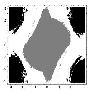
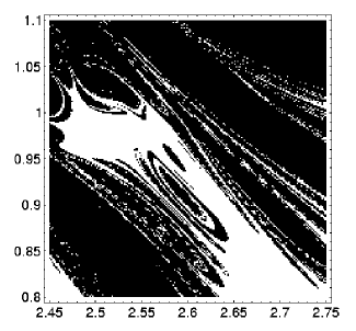
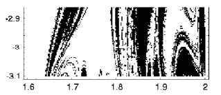
FIG. 3.: Top: The fractal basin boundaries for pairs with $m_{2}/m_{1}=1/3$ and $S_{1}/m_{1}^{2}=S_{2}/m_{2}^{2}=0.6$. All orbits begin with $x_{i}/m=5,\dot{y}_{i}=0.45$. The initial angles $(\theta_{1},\theta_{2})$ are varied. The axes are labelled in radians. $200\times 200$ orbits shown. The middle and bottom panels are details of the upper panel.

Compact pairs with initial conditions drawn from near the fractal basin boundaries will result in unpredictable outcomes. They will have correspondingly unpredictable waveforms. The waveforms for pairs selected from the initial conditions in fig. 3 are shown in fig. 4. The orbits begin with nearly identical initial conditions. Although the difference in initial angles is only $3{}^{o}$, the waveforms are entirely different. The first pair separates while the second pair executes many thousands of orbits.

FIG. 4.: The waveform $h_{+}$ for pairs selected from the initial conditions in fig. 3. Both orbits begin with $\theta_{1}=10{}^{o}$. The left panel began with $\theta_{2}=128{}^{o}$ while the right panel began with $\theta_{2}=131{}^{o}$. The extreme angles were randomly chosen from the fractal set for illustration. Chaos is seen with more temperate angles as in fig. 2.

It should be emphasized that orbits within smooth basins can still be chaotic. Well within the white stable basins, many orbits will precess chaotically as does the orbit of fig. 2. Similarly, many of the escape orbits and the merger orbits will chaotically scatter before reaching their final outcome. Fractal basin boundaries are a fairly blunt tool, insensitive to some manifestations of chaos. Therefore while fractal basin boundaries do prove the dynamics is chaotic, smooth basins are inconclusive.

With the radiative reaction included, the pair goes from an energy conserving scattering system to a dissipative one. In any stability analysis, dissipation must be turned off to distinguish instability to the onset of chaos from instability to merger from simple energy loss. Once the chaos has been identified, radiative back reaction can readily be incorporated and we do so now. Under the effects of dissipation, some orbits will sweep through the chaotic region of phase space as they inspiral. The surface of section is not useful for a dissipative system since the radius of the orbit is shrinking as energy is lost to gravity waves. However, fractal basin boundaries are still effective at identifying extreme sensitivity to initial conditions. Another advantage is that several thousand orbits can be scanned at once. We use this method to show that dissipation does not obliterate the chaos.

As energy is lost the binary pairs tend to coalesce in such a way that $r\rightarrow$merger is an attractor in phase space that can be described by another fractal set. To show this, we again look at an initial condition slice through phase space. We evolve each of these pairs under the influence of the radiative reaction force. We need to color code the initial conditions on the basis of some well defined outcome. Since all pairs considered coalesce, we have to select some other criterion than that used above. We choose to color code the initial location in the $(\theta_{1},\theta_{2})$ plane white if the pair approach merger from below the $z$-axis and black if they approach merger from above the $z$-axis. The resultant fractal is shown in fig. 5. Another criterion could have been selected and in this sense the basin boundaries are crude, as already mentioned, but they are nonetheless powerful at signaling the presence of chaos. The conclusion to draw from this figure is that there is extreme sensitivity to initial spin angles for rapidly spinning, inspiralling $10M_{\odot}$ black hole and $1.4M_{\odot}$ neutron star binaries. The pairs will inspiral along different paths as a result of this sensitivity and therefore will have disparate waveforms. Similar chaotic sets have also been found for different binary mass ratios and orbital parameters.

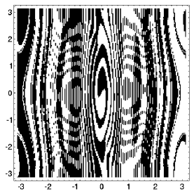
FIG. 5.: The fractal basin boundaries with dissipation included. The parameters are $m_{2}/m_{1}=1.4/10$ and spins $S_{1}=m_{1}^{2}$ and $S_{2}=0.7\ m_{2}^{2}$. The orbits begin with $x_{i}/m=26,\dot{y}_{i}=0.15$ and $z_{i}=0$. The pair can execute anywhere from $0$ to ${\cal O}(40)$ orbits before coalescence. The initial angles $(\theta_{1},\theta_{2})$ are varied from $-\pi$ to $\pi$. $300\times 300$ orbits shown.

This work demonstrates the existence of chaotic regions of phase space. At least some orbits will move into this chaotic region as they inspiral. Of course some orbits will still be regular such as circular inspiral with spins exactly aligned with the orbital angular momentum. A systematic scan of all parameters is needed to ascertain when the dynamics is predictable and regular and when it is chaotic. A quantitative comparison of the waveforms from a chaotic orbit against a circular template is also needed to evaluate how seriously chaos would deter detection. Given that eccentricity in an otherwise simple orbit can greatly diminish the signal when matched against a circular template [21], the chaotic precession does not bode well. Still, the luminosity in gravity waves is enhanced for some of these wilder orbits [5], as was already seen along the regular homoclinic orbits [15]. Though unlikely, an optimist might hope that direct detection of these gravity waves will be possible if the signal is boosted substantially above the noise, relieving the dependence on a theoretical template.

The inherent difficulty in the direct detection of gravity waves highlights the importance of indirect methods of detection. Corroborating evidence for gravity waves in electromagnetic observations may be promising. Chaos can have unexpected benefits if the black hole is able to capture the light from a luminous companion for many chaotic orbits before some of the light escapes. Such chaotic scattering of a pulsar beam around a central black hole could lead to a diffuse glow around the pair [6]. While this signature is likely to be faint, any confirmation of a gravity wave signal will be welcome.

I am grateful to E.J.Copeland, R.O’Reilly, and N.J.Cornish for their valuable input. This work is supported by a PPARC Advanced Fellowship.

REFERENCES

- [1] G. Contopolous, Proc. R. Soc. A431 183 (1990); Proc. R. Soc. A435 551 (1990).
- [2] L.Bombelli and E.Calzetta, Class. Quantum. Grav. 9 2573 (1992).
- [3] S.Suzuki and K.Maeda, Phys. Rev. D. 55 4848 (1997).
- [4] C. P. Dettmann, N. E. Frankel and N. J. Cornish, Phys. Rev. D50, R618 (1994); Fractals, 3, 161 (1995).
- [5] N.J. Cornish and N.E.Frankel, Phys. Rev. D 56 1903 (1997).
- [6] J.Levin, Phys. Rev. D. 60 64015 (1999).
- [7] S.D.Majumdar, Phys. Rev. 72 390 (1947).
- [8] A. Papapetrou, Proc. R. Irish Acad. A51 191 (1947).
- [9] L. Blanchet and T. Damour, Ann. Inst. Henri Poincaré A, 50 377 (1989); T. Damour and B.R. Iyer, Ann. Inst. Henri Poincaré 54 115 (1991).
- [10] T. Damour and N. Deruelle, C. R. Acad. Sci. Paris 293 537 (1981); 293 877 (1981).
- [11] C.M. Will and A.G. Wiseman, Phys. Rev. D 54 4813 (1996).
- [12] A.Gopakumar and B.R.Iyer, Phys. Rev. D. 59 7708 (1997).
- [13] L. Kidder, Phys. Rev. D. 52 821 (1995).
- [14] L.E.Kidder, C.M.Will and A.G.Wiseman, Phys. Rev. D 47 R4183 (1993).
- [15] J. Levin, R. O’Reilly, and E.J. Copeland, gr-qc/9909051.
- [16] E. Ott, Chaos in dynamical systems, (Cambridge University Press, Cambridge, 1993).
- [17] N.J. Cornish and J.J. Levin, Phys. Rev. D 53 3022 (1996).
- [18] N.J. Cornish and J.J. Levin, Phys. Rev. Lett. 78 998 (1997); Phys. Rev. D.55 7489 (1997).
- [19] L.E.Kidder, C.M.Will and A.G.Wiseman, Phys. Rev. D. 47 3281 (1993); D.M Eardly and E.W. Hirschmann, gr-qc 9601019; D.Lai and A.G.Wiseman, Phys. Rev. D. 54 3958 (1996).
- [20] V.Kalogera, astro-ph/9911417.
- [21] K.Martel and E.Poisson, gr-qc/9907006.