Relativistic Scalar Gravity:
A Laboratory for Numerical Relativity[1]

Abstract

We present here a relativistic theory of gravity in which the spacetime metric is derived from a single scalar field $\Phi$. The field equation, derived from a simple variational principle, is a non-linear flat-space four-dimensional wave equation which is particularly suited for numerical evolution. We demonstrate that while this theory does not generate results which are exactly identical quantitatively to those of general relativity (GR), many of the qualitative features of the full GR theory are reproduced to a reasonable approximation. The advantage of this formulation lies in the fact that 3D numerical grids can be numerically evolved in minutes or hours instead of the days and weeks required by GR, thus drastically reducing the development time of new relativistic hydrodynamical codes. Scalar gravity therefore serves as a meaningful testbed for the development of larger routines destined for use under the full theory of general relativity.

]

I Scalar Theories of Gravity

Computational loads in numerical relativity are typically immense. Fox [2] estimates that the computation of the gravitational waves from black hole collisions would require approximately 100,000 hours on a Cray Y-MP. Current [3] improvements in parallel machines and algorithms may cut this to 50 hours on rare machines. It is very difficult to do even test problems under these conditions. Clearly, one cannot wait days or weeks to get results to use in deciphering the cause (or even detecting the existence) of some problem in the code. When one considers that we are not even completely certain what new problems we will be forced to face, the situation is completely unacceptable. While many problems will be unique to the Einstein equations and must be faced in that context, others, notably in relativistic hydrodynamics, will be similar using any metric theory of gravity.

Shapiro and Teukolsky [4] have proposed that instead of starting with the full equations of general relativity, we should instead look at a simpler relativistic theory of gravity in order to discover and learn how to resolve these unknown issues while utilizing far less computational resources than the full problem would require. The scalar theory presented here is intended to provide a testbed for relativistic hydrodynamics. It is to be implemented in code that accepts a matter stress-energy tensor and generates an updated metric at each time step. The hydrodynamic code that accepts this metric and updates the hydrodynamic variables and the stress-energy tensor can be exactly the same code that is to interact in the same way with a program that solves the Einstein equations. Thus speeded development and testing of hydrodynamical codes is the principal motivation for developing this scalar theory. Any gravitational physics or techniques that may be carried over to Einstein equation solvers will be a bonus.

Shapiro and Teukolsky’s prescription is to explore the scalar gravitation theory presented in Exercise 7.1 of Misner, Thorne, and Wheeler (MTW) [5]. This theory, however, violently disagrees with observations and fails all three of the classical tests of general relativity. It is not clear that this theory is close enough to general relativity to prove useful to our purposes. Nevertheless, the potential benefits of a simplified testbed are such that a further examination of scalar gravity theories is warranted.

Ni [6] provides a compendium of metric theories organized in terms of their “Parameterized Post-Newtonian limits” as defined by Thorne and Will [7]. In general, scalar theories can be grouped into three classifications:

1. Conformally flat theories

2. Stratified conformally flat (SCF) theories

3. Other scalar theories

Conformally flat theories are some sense the simplest possible theories of gravity. In this class of theories, the metric takes the form

$$ds^{2}=\Psi(-dt^{2}+dx^{2}+dy^{2}+dz^{2})\quad,$$ (1)

where the variable $\Psi$ is some function of the scalar field $\Phi$, e.g., $\Psi=\exp{2\Phi}$. We use the symbol $\Phi$ throughout for the basic scalar gravitational field, normalized so that in the Newtonian limit it becomes the Newtonian gravitational potential, asymptotically $\Phi=-M/r=-GM/rc^{2}$. We shall also use units with $G=1=c$ where $G$ is the Newton-Cavendish gravitational constant. The field equation (which determines $\Phi$) can technically be anything, but is generally some variation of the scalar wave equation, with some version of the matter density serving as the source term. Ni describes five different examples of this type of theory. [6]

All conformally flat theories (including the theory of MTW Ex.7.1) suffer from a fatal flaw: since Maxwell’s equations are conformally invariant, all conformally flat theories must predict zero light deflection, in obvious disagreement with experiment. Most also fail various other solar-system tests of general relativity, but the zero light-deflection prediction is a fundamental consequence of each of these theories and cannot be avoided.

One way to solve the light-deflection problem is to postulate that there exists a universal preferred reference frame and that while spacelike slices of this spacetime (referred to as “strata”) are conformally flat, the full spacetime is not. The general form for the metric of this “stratified conformally flat theory” is

$$ds^{2}=-\Psi_{1}dt^{2}+\Psi_{2}(dx^{2}+dy^{2}+dz^{2})\quad,$$ (2)

where again $\Psi_{1}$ and $\Psi_{2}$ are functions of the scalar field $\Phi$. This type of metric obviously destroys Lorentz invariance, however this is not as strict a requirement as one might think. Global Lorentz invariance is a treasured philosophical feature of general relativity with asymptotically flat boundary conditions, but in reality we usually model sources as though they existed alone and in isolation in the Universe. The fact that we have a preferred reference frame in this case is not such an important issue.

The last category, more general scalar theories, has seen little examination in the literature and we do not study it here.

II Simple Relativistic Scalar Gravity

A Variational Principle and Metric

We propose a variational principle which leads to a simplified theory closely related to Ni’s [6] “Lagrangian-based stratified theory”, which until 1972 was thought to agree with all tests of general relativity. It has since been found to disagree with the Earth rotation rate experiment [16] and with white dwarf stability observations [8] (although Ni notes that the validity of the latter experiment can be questioned since it is based upon ideas about pulsation-damping forces in white dwarfs which have yet to be tested experimentally). As will be seen in Section II E, the PPN form of the simplified metric is identical to that found from Ni’s theory, hence it satisfies (and fails) the same tests of general relativity as does Ni’s theory. This stratified conformally-flat (SCF) scalar theory, therefore, has all of the advantages of Ni’s more complicated theory, yet has a simpler form which eliminates many of the disadvantages. Additionally, the resulting field equation has the form of the non-linear Klein-Gordon equation, for which a significant amount literature exists, thus aiding in the numerical implementation of the theory.

We begin by selecting the Lagrangian:

$$I=-\frac{1}{8\pi}\int\eta^{\mu\nu}\Phi_{,\mu}\Phi_{,\nu}\sqrt{-\eta}\,d^{4}x+\int{\cal L}_{\rm matter}d^{4}x\quad.$$ (3)

This differs from Ni’s theory (cf. [6] or a summary in MTW [5, Box 39.1]) only in using $\eta^{\mu\nu}$ where Ni uses $g^{\mu\nu}$ in the first term, so that our scalar field $\Phi$ propagates along flat spacetime light cones. Here $\eta^{\mu\nu}$ is the Minkowski metric, and $\sqrt{-\eta}=1$ unless one is using nonstandard, e.g., spherical, coordinates. We generate the metric (with which all nongravitational fields interact just as in general relativity) in the same way as Ni:

$$ds^{2}=-e^{2\Phi}dt^{2}+e^{-2\Phi}(dx^{2}+dy^{2}+dz^{2})\quad.$$ (4)

We have briefly explored alternative forms of the stratified metric,

$$ds^{2}=-(1-\frac{2}{n}\Phi)^{-n}dt^{2}+(1-\frac{2}{n}\Phi)^{n}(dx^{2}+dy^{2}+dz^{2}),$$ (5)

but found that the most realistic (i.e., closest to Einstein) results are obtained when $n$ is allowed to go to infinity.

B The Field Equation

The field equation follows from varying $\Phi$ in the action (3) which gives

$$\frac{\partial}{\partial x^{\mu}}(\sqrt{-\eta}\,\eta^{\mu\nu}\frac{\partial\Phi}{\partial x^{\nu}})=-4\pi\frac{\delta{\cal L}_{\rm matter}}{\delta g_{\mu\nu}}\frac{\partial g_{\mu\nu}}{\partial\Phi}\quad.$$ (6)

The right hand side of this equation can be expressed in terms of the stress-energy tensor by using the definition found in MTW [5, Chap. 21]):

$$\frac{\delta{\cal L}_{\rm matter}}{\delta g_{\mu\nu}}=\mbox{$\frac{1}{2}$}T^{\mu\nu}\sqrt{-g}\quad.$$ (7)

The field equation derived from this variational principle, which is valid for a metric generated in any way from $\Phi$, is therefore

$$\sqrt{-\eta}\,\Box\Phi=-2\pi\sqrt{-g}\frac{\partial g_{\mu\nu}}{\partial\Phi}T^{\mu\nu}\quad,$$ (8)

where $\sqrt{-\eta}\,\Box=\partial_{\mu}\sqrt{-\eta}\,\eta^{\mu\nu}\partial_{\nu}$. Utilizing the SCF metric (4), this field equation becomes

$$\sqrt{-\eta}\,\Box\Phi=4\pi(T^{00}+e^{-4\Phi}\delta_{ij}T^{ij})\quad.$$ (9)

The theory proposed by Ni [6] differs only in using the metric (4) where our simplified theory uses the Minkowski metric $\eta_{\mu\nu}$ on the left hand side.

C Conserved Quantities

It is often important to know which physical quantities are conserved in a theory. These quantities are of particular importance if the field equation is to be solved numerically, as they are often used as to monitor the error or stability of a numerical integration algorithm (e.g. [9]). A conserved energy and conserved linear and angular momentum can be derived from the Lagrangian implicit in the variational principle of (3) using Noether’s Theorem, since this Lagrangian density is invariant under spacetime translations and spatial rotations. Expositions of Noether’s theorems can be found, e.g., in Hill [10] and in Byers [11]. For the present application the special case using the canonical stress-energy tensor suffices. For a Lagrangian density ${\cal L}(\Psi^{\sc A},{\Psi^{\sc A}}_{,\mu})$ which has no explicit coordinate dependence but may contain several fields $\Psi^{\sc A}$, the equations

$${{\cal T}_{\lambda}}^{\gamma}_{,\gamma}=0$$ (10)

where

$${{\cal T}_{\lambda}}^{\gamma}={\cal L}\delta_{\lambda}^{\gamma}-\frac{\partial{\cal L}}{\partial{\Psi^{\sc A}}_{,\gamma}}{\Psi^{\sc A}}_{,\lambda}$$ (11)

are easily shown to be a consequence of the field equations

$$0=\frac{\partial{\cal L}}{\partial{\Psi^{\sc A}}}-\partial_{\gamma}\frac{\partial{\cal L}}{\partial{\Psi^{\sc A}}_{,\gamma}}\quad.$$ (12)

(See, e.g., [12, 13, 14].) Since the stress energy tensor ${{\cal T}_{\lambda}}^{\gamma}$ as defined in equation (11) is linear in $\cal L=L_{\rm grav}+L_{\rm matter}$, it is also a sum of two parts and the energy-momentum conservation law can be written as

$$\left[{{\cal T}_{({\rm grav})\lambda}}^{\gamma}+{{\cal T}_{({\rm matter})\lambda}}^{\gamma}\right]_{,\gamma}=0\quad.$$ (13)

Here

$${{\cal T}_{({\rm grav})\lambda}}^{\gamma}=\frac{1}{4\pi}\sqrt{-\eta}\left(-\mbox{$\frac{1}{2}$}\eta^{\mu\nu}\Phi_{,\mu}\Phi_{,\nu}\,\delta^{\gamma}_{\lambda}+\Phi_{,\lambda}\Phi_{,\mu}\eta^{\mu\gamma}\right)$$ (14)

follows from equation (11) since $\cal L_{\rm grav}$ depends on only the single field $\Phi$. Although $\cal L_{\rm matter}$ may depend on several matter fields, in it $\Phi$ occurs only indirectly via $g_{\mu\nu}$. Since we assume that $\cal L_{\rm matter}$ is generally covariant, one knows that its stress-energy tensor can equivalently be obtained as

$${{\cal T}_{({\rm matter})\lambda}}^{\gamma}=2g_{\lambda\alpha}\frac{\delta{\cal L}_{\rm matter}}{\delta g_{\alpha\gamma}}=g_{\lambda\alpha}\sqrt{-g}\,T^{\alpha\gamma}\quad.$$ (15)

To directly verify the conservation law (13) one uses the scalar field equation (9) and the covariant conservation law for the matter fields ${T^{\lambda\gamma}}_{;\gamma}=0$ in the form

$${{{\cal T}_{({\rm matter})\lambda}}^{\gamma}}_{,\gamma} = \Gamma_{\alpha\lambda\gamma}{{\cal T}_{({\rm matter})}}^{\alpha\gamma}$$ (16)

$$= \mbox{$\frac{1}{2}$}g_{\alpha\gamma,\lambda}\sqrt{-g}\,T^{\alpha\gamma}$$ (17)

$$= -\Phi_{,\lambda}(T^{00}+e^{-4\Phi}\delta_{ij}T^{ij})\quad.$$ (18)

Only the last step in this equation uses the special SCF form (4) of $g_{\mu\nu}$ in terms of $\Phi$.

Since the $\eta^{\mu\nu}$ are constants, the conservation law ${{{\cal T}_{\lambda}}^{\gamma}}_{,\gamma}=0$ can also be written ${{\cal T}^{\lambda\gamma}}_{,\gamma}=0$ by defining ${{\cal T}^{\lambda\gamma}}=\eta^{\lambda\alpha}{{{\cal T}_{\alpha}}^{\gamma}}$. One then defines the total energy and momentum of the system as usual by

$$P^{\mu}=\int{{\cal T}^{\mu 0}}\,d^{3}x$$ (19)

and recognizes ${\cal T}^{0k}$ as the Poynting-like energy flux. The zero-component of (19) is the energy, defined as

$$E\equiv P^{0}=-\int{{\cal T}_{0}^{0}}\,d^{3}x\quad,$$ (20)

with the corresponding energy conservation law

$$\frac{dE}{dt}=-\oint{{\cal T}^{0k}}\,d^{2}\sigma_{k}\quad.$$ (21)

Here ${\cal T}^{0k}=-{{\cal T}_{0}}^{k}\equiv{{\cal S}^{k}}$ is an energy flux like the Poynting vector. In most applications the bounding surface will be chosen outside the region occupied by matter so only the gravitational terms remain as ${\cal S}^{k}_{\rm grav}=-(c^{5}/4\pi G)\Phi_{,0}\Phi_{,k}$.

Angular momentum conservation is a consequence of the symmetry of the stress-energy tensor. The gravitational part of ${\cal T}^{\lambda\gamma}$ is symmetric as a consequence of the Lorentz invariance of the Lagrangian ${\cal L}_{\rm grav}$ from which it is derived, and is also clear from its explicit definition

$${\cal T}_{({\rm grav})}^{\lambda\gamma}=\frac{1}{4\pi}\sqrt{-\eta}\left(-\mbox{$\frac{1}{2}$}\eta^{\mu\nu}\Phi_{,\mu}\Phi_{,\nu}\,\delta^{\lambda\gamma}+\eta^{\lambda\mu}\Phi_{,\mu}\Phi_{,\nu}\eta^{\nu\gamma}\right)\ \ .$$ (22)

However the matter Lagrangian is not Lorentz invariant in view of the preferred rest frame in which equation (4) holds. The matter stress-energy is defined by

$${{\cal T}_{({\rm matter})}}^{\lambda\gamma}=2\eta^{\lambda\beta}g_{\beta\alpha}\frac{\delta{\cal L}_{\rm matter}}{\delta g_{\alpha\gamma}}=\eta^{\lambda\beta}g_{\beta\alpha}\sqrt{-g}\,T^{\alpha\gamma}$$ (23)

and does not inherit the symmetry of $T^{\alpha\beta}$ except in its spatial components: ${{\cal T}_{({\rm matter})}}^{ij}={{\cal T}_{({\rm matter})}}^{ji}=e^{-4\Phi}T^{ij}$ . An angular momentum density can be defined as usual ${\cal M}^{\mu\nu\gamma}=x^{\mu}{\cal T}^{\nu\gamma}-x^{\nu}{\cal T}^{\mu\gamma}$ which satisfies ${{\cal M}^{\mu\nu\gamma}}_{,\gamma}={\cal T}^{\nu\mu}-{\cal T}^{\mu\nu}$ so that a conserved angular momentum is defined

$$J^{ij}=\int{{\cal M}^{ij0}}\,d^{3}x\quad.$$ (24)

D The Newtonian Limit

In order to find the Newtonian limit for this theory, assume a static point source of mass $M$ for the stress-energy tensor and solve the field equation for the Schwarzschild-like solution. The field equation with this source is

$$\bigtriangledown^{2}\Phi=4\pi M\delta(x)\quad.$$ (25)

Away from the source, the solution to this equation is

$$\Phi=-\frac{M}{r}\quad,$$ (26)

which is, of course, the Newtonian potential. The spacetime metric is therefore

$$ds^{2}=-e^{-{2M}/{r}}dt^{2}+e^{{2M}/{r}}(dx^{2}+dy^{2}+dz^{2})\quad.$$ (27)

The small-$\Phi$ (small $M$ or large $r$) limit of the $g_{00}$ component is $g_{00}\rightarrow-(1+2\Phi)$, therefore correspondence with Newtonian gravity is assured.

E PPN Parameters

Having found the field equation, one is now compelled to ask, how “good” is the theory? We will explore a number of definitions of “good” in this paper, but one possible definition is to insist that a “good” theory have parameterized post-Newtonian (PPN) parameters which 1) satisfy as many as possible of the solar system gravitational tests made to date, and 2) match as closely as possible the PPN parameters of general relativity. One must keep in mind, however, that obviously a theory may be “good” in its Newtonian limit yet still give results which differ greatly from general relativity in the strong-field limit! In fact, we have found no solutions in this SCF scalar theory that approximate the cosmological models in general relativity.

Ni [6] has calculated the PPN parameters for his “Lagrangian-based stratified theory”, which our simplified theory closely resembles. Subtracting the present field equation (9) from Ni’s shows that the theories differ by

$$(\sqrt{-g}\, g^{\mu\nu} )_{,\mu}\Phi_{,\nu}-(\sqrt{-\eta}\,\eta^{\mu\nu})_{,\mu}\Phi_{,\nu}$$ (28)

$$= 4e^{-4\Phi}(\Phi_{,0})^{2}+(1-e^{-4\Phi})\Phi_{,00}\quad.$$ (29)

Both of these terms are $O(c^{-6})$. Because the PPN formulation considers terms through $O(c^{-4})$, this theory and Ni’s must have identical PPN parameters. [The PPN approximation is often considered an expansion in powers of $1/c$ since the dimensionless quantities $(v/c)^{2}$ and $GM/rc^{2}$ are of comparable size (virial theorem) in bound systems, and timelike derivatives $\partial_{0}$ are smaller by a factor of order $v/c$ than space derivatives $\partial_{i}$ when the time dependence is generated by the motion of sources. The Newtonian potential $\Phi\sim-GM/rc^{2}$ is considered to be $O(c^{-2})$.] The PPN parameters for this theory [6] are therefore

$$\xi=\eta=0,\gamma=\beta=\beta_{1} = \beta_{2}=\beta_{3}=\beta_{4}=\Delta_{2}=1,$$ (30)

$$\Delta_{1} = -\frac{1}{7}\quad.$$ (31)

The theory agrees with general relativity with the exception of the $\Delta_{1}$ parameter. Additionally, due to its value of $\Delta_{1}$, it disagrees with the Earth rotation rate experiments. [16] Essentially, this theory predicts an incorrect relative amount of dragging of inertial frames ($g_{0i}$) produced by unit momentum ($\rho v$) (see MTW Box 39.2 [5]). On the basis of PPN parameters, this theory compares favorably to all of its scalar gravity competitors. In fact, one obtains precisely the PPN parameters of Ni’s SCF theory [6] and Rosen’s [17] two field variable theory with $\lambda=1$, yet both authors postulate a considerably more complex field equation than is used here.

III The Schwarzschild-like Solution

The PPN formulation predicts how the mid-range field of scalar gravity compares to general relativity, but it makes no such prediction about the strong-field region. A second measure of how “good” the theory is, then, is to calculate the analytic results for a simple strong-field case and compare those results to the equivalent case in general relativity. The metric found in Section II D corresponds to the well-studied Schwarzschild case of GR; in this section we will determine the properties of the equivalent case for scalar gravity, studying geodesics in a manner parallel to §25.3 of MTW [5].

A The Effective Potential

To begin, write (27) in spherical coordinates

$$ds^{2}=-e^{-{2M}/{r}}dt^{2}+e^{{2M}/{r}}dr^{2}+r^{2}e^{{2M}/{r}}d\theta^{2}\quad.$$ (32)

The geometry is unaffected by changes in $t$ or $\theta$, therefore two constants of motion exist:

$$p_{0}=-E\quad,\quad p_{\theta}=\pm L\quad.$$ (33)

Conservation of rest-mass energy,

$$g_{\alpha\beta}\,p^{\alpha}p^{\beta}+\mu^{2}=0\quad,$$ (34)

gives the orbit equation

$$-E^{2}e^{{2M}/{r}}+e^{{2M}/{r}}\left(\!\frac{dr}{d\lambda}\!\right)^{2}+\left(\frac{L}{r}\right)^{2}e^{-{2M}/{r}}+1=0$$ (35)

where $\lambda$ is the path parameter and $p^{r}\equiv dr/d\lambda$. Defining $\tilde{E}={E}/{\mu}$, $\tilde{L}={L}/{\mu}$, $\lambda={\tau}/{\mu}$ places the orbit equation in its final form

$$\left(\frac{dr}{d\tau}\right)^{2}=\tilde{E}^{2}-V_{\rm eff}(r)^{2}\quad,$$ (36)

where $V_{\rm eff}$, the effective potential, is defined as

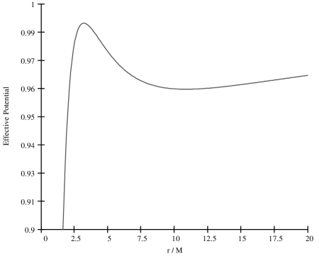
FIG. 1.: The effective potential (37) plotted as a function of $r/M$ for a typical specific angular momentum, in this case $\tilde{L}=4M$. Notice the “pit in the potential”, (see MTW [5, Chap.25]) which gives rise to an innermost stable circular orbit when, for still smaller values of $\tilde{L}$, the stable and unstable circular orbit radii (local min and max of $V_{\rm eff}$) coincide. (see Section III B).

$$V_{\rm eff}(r)^{2}=e^{-{2M}/{r}}\left(\frac{\tilde{L}^{2}}{r^{2}}e^{-{2M}/{r}}+1\right)\quad.$$ (37)

Figure 1 shows a typical plot of the effective potential as a function of $r$.

B Innermost Stable Circular Orbit

One of the first relativistic effects to be noticed was the “pit” in the effective potential, the existence of which implies the presence of an innermost stable circular orbit. Any particle that moves within this limit must necessarily spiral in and impact the singularity at r=0. As the present theory also possesses this pit, it is reasonable to suppose that it possesses an innermost stable circular orbit as well.

Circular orbits occur at extrema of the effective potential. Taking the derivative with respect to $r$ of (37) returns, after some algebra, the circular orbit angular momentum as a function of $r$:

$$\tilde{L}_{\rm circ}=re^{{M}/{r}}\sqrt{\frac{M}{r-2M}}\quad.$$ (38)

It can immediately be seen that no circular orbits exist at all below $r=2M$. The innermost stable circular orbit occurs at the value of $r$ for which $\tilde{L}_{\rm circ}$ is a minimum. Taking the derivative of (38) with respect to $r$ yields

$$r_{\rm isco}=M(3+\sqrt{5})\quad.$$ (39)

This result compares favorably to the predictions of general relativity. GR predicts the innermost stable circular orbit occurs at $r=6M$, which corresponds to a circumference of $12\pi M$. The circumference of the innermost stable circular orbit under the scalar gravity theory is $12.6759\pi M$, a difference of only $5.63\%$

Well inside the innermost stable circular orbit we cannot expect this theory to mimic general relativity. To produce the analog of the interior Schwarzschild solutions would require inclusion of the $e^{-4\Phi}\delta_{ij}T^{ij}$ term in equation 9 and the hydrostatic fluid equations, so it is possible that the theory would give a maximum neutron star mass. But since the radial null vectors are $k_{\pm}=\partial_{t}\pm e^{2\Phi}\partial_{r}$, the only possibility for a black hole effect would be to find solutions where $\Phi\rightarrow-\infty$ at a nonzero value of $r$.

IV Gravitational Radiation

With the completion of the LIGO gravitational wave interferometer nearing, attention in the numerical relativity community has been focused upon the production of gravitational wave templates to supply LIGO’s matched-filtering analysis routines. A third and particularly relevant measure of how “good” scalar gravity is would be to calculate the frequency of the radiation, as observed at infinity, of the innermost stable circular orbit.

From the scalar gravity Schwarzschild-like metric

$$ds^{2}=-e^{-{2M}/{r}}dt^{2}+e^{{2M}/{r}}dr^{2}+r^{2}e^{{2M}/{r}}(d\theta^{2}+\sin{\theta}^{2}d\phi^{2})$$ (40)

the radiation frequency, $2\omega$, can be defined from the circular orbit frequency

$$\omega=\frac{d\phi}{dt}=\frac{d\phi}{d\tau}\frac{d\tau}{dt}=e^{-{4M}/{r}}\frac{\tilde{L}}{\tilde{E}r^{2}}\quad.$$ (41)

Combining (37) and (38), yields the effective potential as a function of orbital radius; this value, by (36), is also equal to the orbital energy squared. The result of this algebra is

$$\tilde{E}_{\rm circ}=e^{-{M}/{r_{\rm circ}}}\sqrt{\frac{r_{\rm circ}-M}{r_{\rm circ}-2M}}\quad.$$ (42)

A somewhat more useful quantity conceptually, however, is the binding energy,

$$\tilde{E}_{\rm binding}=1-\tilde{E}_{\rm circ}\quad.$$ (43)

Substituting (42) and (38) into (41) gives, after some algebra, scalar gravity’s equivalent of Kepler’s Third Law

$$\omega^{2}r_{\rm circ}^{2}e^{{4M}/{r_{\rm circ}}}(r-M)=M\quad.$$ (44)

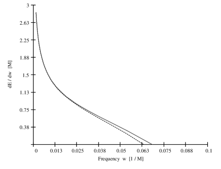
FIG. 2.: The frequency spectrum of gravitational radiation produced by a test mass in nearly circular orbit about a central object as the test mass adiabatically spirals inward. The graph shows the change in binding energy (43) as a function of circular orbit frequency (41), which is in turn a function of the circular orbit radius. The solid line shows the spectrum for a test mass moving within a Schwarzschild background metric, while the dashed line shows the spectrum for a test mass moving within the background metric of (40). The innermost stable circular orbit occurs where each curve crosses the $x$-axis. The agreement between the curves is very good almost down to this point.

Notice that this expression is precisely Kepler’s Third Law only for large ${r}/{M}$. Although $\tilde{E}_{\rm binding}(\omega)$ cannot be found as an analytic expression, we can easily plot the spectrum of the gravitational radiation $d\tilde{E}_{\rm binding}(\omega)/d\omega$ by knowing both $d\tilde{E}_{\rm binding}(\omega)/d\omega=(d\tilde{E}_{\rm binding}(\omega)/dr_{\rm circ})/(d\omega/dr_{\rm circ})$ and $\omega$ as functions of $r_{\rm circ}$. Figure 2 compares the frequency spectrum calculated under scalar gravity with that found from general relativity. As can be seen, the two theories agree quite well almost down to the innermost stable circular orbit. The frequency of the innermost stable circular orbit is found using (44) evaluated at $r=r_{\rm isco}=M(3+\sqrt{5})$:

$$\omega_{\rm isco}=\frac{0.0633326}{M}\quad.$$ (45)

General relativity gives a value of $\omega_{\rm isco}=0.0680414/M$ (a difference of $6.92\%$), again demonstrating the close agreement the two theories. This close agreement is not too surprising when one considers that there is a sense in which the Schwarzschild-like solution of this SCF scalar theory “almost” satisfies Einstein’s equations. The non-zero components of the Einstein tensor, calculated using the metric (40) are

$$G^{0}_{0}=-G^{1}_{1}=G^{2}_{2}=G^{3}_{3}=e^{-2M/r}\frac{M^{2}}{r^{4}}\quad,$$ (46)

rather than zero. This is smaller than the nonzero components of the Riemann tensor in the Schwarzschild metric by a factor $e^{-2M/r}(M/r)$. A dimensionless measure of this failure to satisfy Einstein’s equations has its maximum at $r=M$ where each nonzero component $M^{2}|G^{\mu}_{\nu}|$ is $e^{-2}=0.135$, from which point they decrease monotonically. At $r=r_{\rm isco}$ this error is $0.0009$ and decreases rapidly farther out.

V Discussion

The scalar theory presented here is intended as a stand-in for general relativity while developing hydrodynnamic computer codes for application in problems such as the production of gravitational radiation by binary neutron star systems. It has the advantage of involving only one field variable $\Phi$ (and its time derivative) and satisfying a simple field equation. The field equation (9) involves only the usual flat spacetime d’Alembertian (nonlinearities only in terms containing no derivatives) and reduces to the flat space linear wave equation outside the region occupied by matter. This should simplify its numerical treatment, and particularly the imposition of outgoing wave boundary conditions; there are no curved light cones to manage. Its interface to hydrodynamics can be identical that of general relativity — it requires a matter stress-energy tensor and produces a metric.

It seems plausible that, in a range including fields stronger than those treated by the PPN methods, this theory could also give results that are close to those of general relativity. For Coulomb-like gravitational fields our study of the analog of the Schwarzschild metric shows results within a few percent of those of GR down to the innermost stable circular orbit. For gravitomagnetic forces (from metric components $g_{0i}$ generated by matter currents $\rho v$) it will necessarily fail, as it allows no $g_{0i}$ metric components. Thus one cannot expect physically plausible results when matter velocities approach the velocity of light. But since this scalar theory does reproduce important qualitative features of general relativity (the existence of an innermost stable circular orbit for test particles), it may allow the initial study of important relativistic hydrodynamical phenomena whose accurate analysis will have to be done using the full Einstein theory of gravitation.