Robust test for detecting non-stationarity in data from gravitational wave detectors

Abstract

It is difficult to choose detection thresholds for tests of non-stationarity that assume a priori a noise model if the data is statistically uncharacterized to begin with. This is a potentially serious problem when an automated analysis is required, as would be the case for the huge data sets that large interferometric gravitational wave detectors will produce. A solution is proposed in the form of a robust time-frequency test for detecting non-stationarity whose threshold for a specified false alarm rate is almost independent of the statistical nature of the ambient stationary noise. The efficiency of this test in detecting bursts is compared with that of an ideal test that requires prior information about both the statistical distribution of the noise and also the frequency band of the burst. When supplemented with an approximate knowledge of the burst duration, this test can detect, at the same false alarm rate and detection probability, bursts that are about 3 times larger in amplitude than those that the ideal test can detect. Apart from being robust, this test has properties which make it suitable as an online monitor of stationarity.

I Introduction

Each of the large interferometric gravitational Wave detectors that are now under construction (LIGO [2], VIRGO [3], GEO [4], TAMA [5]) will produce a flood of data when they come online in a few years. Apart from the “main” data channel carrying measurement of strain in the arm lengths, there will be a few hundred auxiliary channels [6] at each site associated with system and environmental monitors, such as seismometers and magnetometers. Their role would be to monitor the state of the detector and its environment so that any unusual event in the main channel or an unexpected behavior of the detector can be diagnosed properly. (The sum total of raw data from the LIGO detectors will be produced at the rate of $\sim 10$ megabytes [7] every second.)

Under ideal conditions, each data channel would carry stationary noise. For the main channel, this would reflect a steady state of the interferometer and for the auxiliary channels, a steady state of the environment. However, experience with prototypes as well as with the several resonant mass detectors that have been operating for quite some time shows that this situation does not hold in reality. There will always be episodes of non-stationarity though their rates and durations will depend on the choice of the detector site and other factors.

Detecting non-stationarity is important both in the main channel, because some non-stationarity could be of astrophysical origin, and also in the auxiliary channels where it can be an important diagnostic of the instrument or its environment. It is also important when estimating a statistical model of the detector noise where it is essential that the data segment used be stationary. [The deleterious effects of non-stationarity on power spectral density (PSD) estimation were noted in [8].]

Several methods for detecting non-stationarity that are relevant in this context have already been considered in the gravitational wave data analysis literature [9, 10]. However, these methods share an unsatisfactory feature which is that the computation of the detection threshold corresponding to a specified false alarm rate requires an a priori knowledge of a statistical model of the stationary ambient noise. An error in the model leads to an error in our knowledge of the false alarm rate. In the real world such prior models are usually not available and it is necessary to estimate noise models from the data itself. Even if a model exists, it will almost always have some free parameters (the variance being a trivial example) whose values would have to be estimated from the data fairly regularly, especially in the case of a complicated instrument such as a laser interferometer or its environment monitors.

Thus, when confronted with an uncharacterized dataset, an experimenter who is only limited to methods such as the above can face considerable uncertainty in fixing a threshold for the test before analyzing the data. For a sufficiently small dataset, the analyst can start with ad hoc thresholds and work in some iterative sense towards a statistically satisfactory conclusion. The problem becomes more serious when the data set to be analyzed is so large that it becomes necessary to substantially automate the analysis, as would most certainly be needed in the case of the large interferometers. An additional set of problems will arise when analyzing auxiliary channels since ambient terrestrial noise may be intrinsically more difficult to characterize and have a variable nature.

We introduce here, in the context of gravitational wave data analysis, a test for detecting non-stationarity for which the issue of fixing the correct threshold is trivial by design. The false alarm rate for such a robust test depends weakly on the statistics of the ambient noise and is specified almost completely by the detection threshold alone. In the present paper we concentrate on short duration non-stationarity or bursts since they are likely to be the most common types of non-stationarity in gravitational wave detectors. We find that the robustness of the test improves for smaller false alarm rates, which is precisely the regime of interest. If required, the test can be optimized in terms of the duration of the bursts that need to be detected.

We compare the efficiency of this test in detecting narrowband bursts with that of an ideal test which requires both a noise model and prior knowledge of the frequency band (center frequency and bandwidth) in which the bursts occur. We find that supplementing our test with an approximate prior knowledge of the burst duration allows it to detect, at the same false alarm rate and detection probability, bursts with a peak amplitude that is a factor of $\sim 3$ larger than that of the bursts which the ideal test can detect.

Apart from being robust, it also has the following properties that make it useful as an online monitor of stationarity. The computational cost associated with this test is quite small. Areas of non-stationarity are clearly distinguished, in the time-frequency plane, from areas of stationarity. Apart from making the output simple to understand visually, this will allow an automated routine to catalogue burst information such as the time of occurrence and frequency band.

The detection of non-stationarity has been actively studied in Statistics for quite some time [14] and numerous tests suitable for a wide variety of non-stationary effects exist in the literature. The central idea behind our test is the detection of statistically significant changes in the PSD. As a means of detecting non-stationarity, this idea is quite natural and has been proposed in several earlier works. (See, for instance,[15, 16].) though what constitutes a change and how it is measured can be defined in many different ways leading to tests that differ statistically as well as computationally. The specific implementation presented in this paper leads to a statistically robust test. The issue of robust tests for non-stationarity, though important as we have argued, has not been considered in gravitational wave detection so far. The same concerns as well as a more rigorous treatment exist in the Statistical literature [17]. Our present work was, however, done independently and this test is a new contribution.

The paper is organized as follows. In Section II we formally state the problem addressed in this paper. Section III describes the Student t-test which lies at the core of our test. This is followed by a discussion of the basic ideas that lead to the test and why the test can be expected to be robust. In Section IV, the test is characterized statistically in term of its false alarm rate and detection power. The main results of this paper are also presented in this section. The computational cost associated with this test is discussed in Section IV D. This is followed by our conclusions and pointers to future work in Section V.

II Formal statement of the problem

A random process $x(t)$ is said to be strictly stationary [11] if the joint probability density $P(x(t_{i}),x(t_{i}+\delta_{1}),x(t_{i}+\delta_{2}),\ldots,x(t_{i}+\delta_{n}))$ of any finite number, $n$, of samples is independent of $t_{i}$. Often, one uses a less restrictive definition called wide sense stationarity which demands only that the mean ${\rm E}\left[x(t_{i})\right]$ and the autocovariance ${\rm E}[(x(t_{i})-{\rm E}[x(t_{i})])(x(t_{i}+\tau)-{\rm E}[x(t_{i}+\tau)])]$ be independent of $t_{i}$. A random process not satisfying any of the above definitions is called non-stationary.

We assume that the ambient noise in the data channel of interest is wide sense stationary over sufficiently long time scales and a burst is an episode of non-stationarity with a much smaller duration. That is, the occurrence of a burst lasting from $t=t_{0}$ to $t=t_{1}$ in a segment $x(t)$ of data ($0\leq t\leq T$) means that

$$x(t)=\left\{\begin{array}[]{lr}\mbox{wide sense stationary}&0\leq t\leq t_{0}\\ \mbox{non-stationary}&t_{0}\leq t\leq t_{1}\\ \mbox{wide sense stationary}&t_{1}\leq t\leq T\end{array}\right.\;,$$ (1)

where $t_{1}-t_{0}\ll T$. In practice, only a time series ${\bf x}$ consisting of regularly spaced samples of $x(t)$ is available instead of $x(t)$ itself. Thus, given the time series ${\bf x}$, we want to decide between the following two hypotheses about ${\bf x}$ :

1. Null Hypothesis $H_{0}$ : ${\bf x}$ is obtained from a wide sense stationary random process.

2. Alternative Hypothesis $H_{1}$ : ${\bf x}$ is obtained from a non-stationary random process.

The frequentist approach [12] to this decision problem, which is followed here, begins by constructing a function ${\cal T}({\bf x})$, called a test statistic, of the data ${\bf x}$. If the data ${\bf x}$ is such that ${\cal T}({\bf x})\geq\eta$, for some threshold $\eta$, the null hypothesis is rejected in favor of the alternative hypothesis for that ${\bf x}$.

Since ${\bf x}$ is obtained from a random process, there exists a finite probability, that ${\cal T}({\bf x})$ crosses the threshold even when the data is stationary. Such an event is called a false alarm and the rate of such events over a sequence of data ${\bf x}$ is called the false alarm rate. The threshold $\eta$ is determined by specifying the false alarm rate that the analyst is willing to tolerate.

To compute the threshold, we need to know the distribution function of ${\cal T}({\bf x})$ when $H_{0}$ is true. This distribution can, in principle, be obtained if the joint distribution of ${\bf x}$ (i.e., a noise model) is known. However, as mentioned in the introduction, such prior knowledge is usually incomplete, if it exists at all, in the real world. The only solution then is to estimate the joint distribution from the data itself. Therefore, one must first find a stationary segment of the data, by detecting and then rejecting non-stationary parts, but that brings us back to our primary objective itself!

To get around this paradox, we must construct ${\cal T}({\bf x})$ such that its distribution is as independent as possible of the distribution of the data under the null hypothesis. If the distribution of the test statistic is strictly independent of the distribution of ${\bf x}$, the test is called [13] non-parametric. If the test statistic distribution depends on the distribution of ${\bf x}$ but only weakly, the test is said to be a robust test. Tests which do not have either of these properties are called parametric. Formally, therefore, the aim of this work is to find a non-parametric, or at least a robust test, for non-stationarity.

III Description of the test

A Student’s $t$-test

Before we describe our test for non-stationarity, it is best to discuss Student’s t-test [13] in some detail since this standard statistical test plays an important role in what follows.

Student’s t-test is designed to address the following problem. Given a set of $N$ samples, $\left\{x_{1},\ldots,x_{N}\right\}$, drawn from a Gaussian distribution of unknown mean and variance, how do we check that the mean $\mu$ of the distribution is non-zero? In Student’s t-test, a test statistic $t$ is constructed,

$$t=\frac{\widehat{\mu}\sqrt{N}}{\sqrt{\widehat{s}^{2}}}\;,$$ (2)

where

$$\widehat{\mu} := \frac{1}{N}\sum_{j=1}^{N}x_{j}\;,$$ (3)

$$\widehat{s}^{2} := \frac{1}{N-1}\sum_{j=1}^{N}\left(x_{j}-\widehat{\mu}\right)^{2}\;.$$ (4)

The distribution of $t$ is known [18], both when $\mu=0$ and $\mu\neq 0$. To check whether $\mu\neq 0$, a two-sided threshold is set on t corresponding to a specified false alarm probability. If t crosses the threshold on either side, the null hypothesis $\mu=0$ is rejected in favour of the alternative hypothesis $\mu\neq 0$.

Of interest to us here are two main properties of the t-test. First, if two sets of independent samples $X=\left\{x_{1},\ldots,x_{N}\right\}$ and $Y=\left\{y_{1},\ldots,y_{N}\right\}$ are drawn from Gaussian distributions with the same but unknown variances, the t-test can be employed to check whether the means of the two distributions are equal or not. This can be done simply by constructing a third set of samples $Z=\left\{y_{1}-x_{1},\ldots,y_{N}-x_{N}\right\}$, which would again be Gaussian distributed, and then testing, as shown above, whether the mean of the distribution from which $Z$ is drawn is non-zero or not.

The second important property [19] of the t-test is its robustness : As long as the underlying distributions from which the two samples are drawn are identical, but not necessarily Gaussian, the distribution of the t statistic does not deviate much from the Gaussian case. The lowest order corrections to the mean and variance of the distribution being ${\cal O}(N^{-5/2})$ and ${\cal O}(-N^{2})$ respectively.

B An outline of the test

We present here an outline of our test. The details of the actual algorithm are presented in the appendix.

From Sec. II, it is clear that a direct signature of non-stationarity is a change in the autocovariance function. This implies that the PSD of the random process should also change since the it is the Fourier transform of the autocovariance function [11]. Therefore, the basic idea behind our test is the detection of a change in the PSD of a time series.

The test involves the following steps (see Fig. 1 also).

1. The time series to be analyzed is divided into adjacent but disjoint segments of equal duration $l_{l}$.

2. Take two such disjoint data segments $S_{k}$ and $S_{k+\epsilon}$ separated by a time interval $(\epsilon-1)\,l_{l}$, $\epsilon=1,\,2,\,\ldots$. We would like to compare the PSDs of these two segments and test if there is a significant difference.

3. Subdivide each of the two segments into $N$ subsegments of equal duration. Thus, segment $S_{i}$, $i\in\left\{k,\,k+\epsilon\right\}$, gives us $N$ subsegments, each of duration $l_{s}=l_{l}/N$, which we denote by $s^{(i)}_{j}$, $j=1,\,2,\ldots,N$. This is an intermediate step in the estimation of the PSD of each segment $S_{i}$.

4. Compute the periodogram of each $s^{(i)}_{j}$. A periodogram is the squared modulus of the Discrete Fourier Transform (DFT) of a time series [Eq. (6].

5. For every frequency bin, therefore, we obtain a set $X$ of $N$ numbers from $S_{k}$ and similarly another set $Y$ from $S_{k+\epsilon}$. In a conventional estimation of the PSD of a segment, say $S_{k}$, we would simply average the corresponding set $X$. However, since we want to compare two PSDs, we do the following instead.

6. Perform Student’s t-test for equality of mean on these two independent sets $X$ and $Y$. If the t statistic crosses a preset threshold $\eta$, then a significant change in the mean is indicated, otherwise not.

7. Repeat step 6 for all frequency bins in exactly the same manner.

Steps 2 to 7 should then be repeated with another pair of disjoint segments $S_{k+1}$ and $S_{k+\epsilon+1}$ and so on.

Thus, the output of the test at this stage is a two dimensional image with time along one axis and frequency along the other. In this image, every frequency bin for which the threshold $\eta$ is crossed can be thought of as being colored black while the remaining are colored white. Hence, white areas in this image would indicate stationarity while the contrary would be indicated by the black areas. A sample image is shown in Fig. 2(a). It is the result of applying the test to a simulated time series constructed by adding a broad band burst to stationary white Gaussian noise (see Sec. IV A for definitions).

Not all black areas would, however, correspond to non-stationarity. Most of them would be random threshold crossings caused by the stationary noise itself. We search, therefore, for clusters of black pixels in the image which pass a veto that can be motivated as follows. Suppose the burst is fully contained in one segment, say, $S_{k}$. Then one would expect the t-test threshold to be crossed once when comparing $S_{k}$ with $S_{k-\epsilon}$ and again when $S_{k}$ is compared with $S_{k+\epsilon}$. This leads to a characteristic “double bang” structure for the cluster of black pixels. We throw away all other groups of black pixels that do not show such a feature. (This scheme is defined rigorously in the appendix.) Fig 2(b) shows the result obtained by applying this veto to the image in Fig 2(a). One of the cluster is at the location of the added burst while the other is a false event.

C Why is this test robust?

This test can be expected to be robust for two reasons. First, the periodogram at any frequency is asymptotically exponentially [20, 21] distributed. This can be heuristically explained as follows. The DFT of a time series is a linear transform. If the number of time samples in a random time series is sufficiently large, it then follows from the central limit theorem that the DFT of that time series will have, at each frequency, imaginary and real parts which are distributed as Gaussians. Since the basis functions used in a DFT are orthogonal, the real and imaginary parts also tend towards being statistically independent. This implies that, for a sufficiently large number of time samples, the periodogram, which is simply the squared modulus of the DFT, is exponentially distributed at each frequency.

The second reason which should make the test robust is the fact, mentioned earlier, that the t-test is robust against non-Gaussianity when the two samples being compared have identical distributions. Under the null hypothesis of stationarity, we do indeed have identically distributed sets in our case.

Since the asymptotic distribution of a periodogram is independent of the statistical distribution of the time samples, much of the information about the time domain statistical distribution is lost in the frequency domain. Thus, the t-test “sees” nearly exponentially distributed samples whereas the time domain samples may have a Gaussian or Non-Gaussian distribution. Added to this, the robustness of the t-test also removes information about the time domain statistical distribution. Further, the t-test checks for a change in the mean value and is insensitive to the absolute value of the mean. This is strictly true in the Gaussian case but, because of the robustness of the t-test, it should also hold to a large extent for the exponential case.

These basic considerations suggest strongly that the test as a whole should be robust. However, the test also involves some other steps beyond just a simple t-test. First, the same segment is involved twice in a t-test (c.f. Sec. III B). Thus, for any $k$, samples $k$ and $k+\epsilon$ in the sequence of t values at a given frequency will be correlated to a large extent. Second, we impose a non-trivial veto.

The above features of the test, though well motivated and conceptually simple, make a straightforward analytical study of the test difficult. Therefore, to establish the robust nature of the test and quantify its performance, we must follow a more empirical approach based on Monte Carlo simulations. This is the subject of the next section. An analytical treatment of the test is currently under development.

IV Statistical characterization of the test

Our main aim in this section is to demonstrate the robust nature of the test and to study the efficacy of this test in detecting non-stationarity. Since, we need to use Monte Carlo simulations for understanding these statistical aspects of the test, we discuss only a few selected cases in this paper.

For a test to qualify as robust the threshold should be almost completely specified by the false alarm rate without requiring any assumptions about the statistics of the data. The false alarm rate, in the context of this test, is the rate at which clusters of black pixels occur when the input to the test is a stationary data stream. To obtain the false alarm rate, several realizations of stationary noise are generated and the test is performed on each. For a given threshold, the number of clusters detected over all the realizations provides an estimate of the false alarm rate at that threshold.

The efficacy of a test in detecting a deviation from the null hypothesis is measured by the detection probability of the deviation. In this paper, we measure the detection probability of different types of bursts that appear additively in stationary ambient noise. Realizations of signals from a fixed class (such as narrowband or broadband bursts of noise) are generated, to each of which we add a realization of stationary noise. The test is applied to the total data and we check whether a cluster of black pixel appears in a specified area of the time-frequency plane. This fixed area, which we call the detection region, is specified in advance of the simulation. The ratio of the number of realizations having a cluster in the specified area to the total number of realizations gives an estimate of the detection probability for bursts of that class.

The function that maps the test threshold into false alarm rate depends on the test parameters, $l_{l}$, $l_{s}$ and $\epsilon$ (c.f. Sec. III B). Therefore, for each choice of these test parameters, the test must be calibrated separately using a Monte Carlo simulation. However, thanks to the robust nature of the test, the simulation needs to be performed only once and for a simple noise process such as Gaussian white noise which need not have any relation to the actual random process at hand. The role of the test parameters is discussed in more detail in Sec. IV C.

A False alarm probability

We perform a Monte Carlo simulation for each of the representative cases below and show that the false alarm rate, as a function of threshold, is the same for all of them.

Each realization of the input data is a 10 sec long time series and each simulation uses $5000$ such realizations. We can look upon all the separate realizations of the input as forming parts of a single data stream ($5000\times 10$ sec long) and, if we assume that false alarms occur as a Poisson process, the false alarm rate (in number of events per hour) is given by the total number of false alarms over all realizations divided by $5\times 10^{4}/3600$.

The various cases considered here are as follows.

(i) White Gaussian noise ($\sigma=1$)— The time series consists of independent and identically distributed Gaussian random variables. The standard deviation $\sigma$ of the Gaussian random variables is unity and their mean is zero.

(ii) White Gaussian noise ($\sigma=10$) — Same as above but with $\sigma=10$.

(iiI) White non-Gaussian noise — All details in this simulation are the same as above except that the distribution of each sample is now chosen to be an exponential with $\sigma=1$.

(iv) Colored noise — We generated Gaussian, zero mean noise with a PSD as shown in Fig. 3. The overall normalization is arbitrary but the noise is scaled in the time domain to make its variance unity. This PSD was derived from the expected initial LIGO PSD, as provided in [22], by truncating the latter below 5 Hz and above 800 Hz followed by the application of a band pass filter with unity gain between 50 Hz and 500 Hz.

The range covered by the above types of statistical models is much more extensive than would be required in practice. By applying the test to such extreme situations, we can bound the variations in the false alarm rate versus threshold curve that would occur in a more realistic situation. In considering this range of models for the stationary background noise, we have gone from a two-sided distribution to a completely one side distribution. The output from most channels would be two sided and, hence, closer to a Gaussian than the Exponential distribution considered here.

The results are shown in Fig. 4, 5 and 6. For the small false alarm rates ($<5$/hour) that will be required in practice, the test is clearly shown to be very insensitive to the statistical nature of the data. The largest variation is between the Gaussian and exponential case while there is hardly any variation, even at large false alarm rates, among the Gaussian cases. The variation between the Gaussian and exponential case is less than $\sim 50\%$ in the worst case. As explained above, this should be treated as an upper bound on the error one might expect in practice.

Figs. 4, 5 and 6 correspond to different sets of test parameter values. The threshold for a given false alarm rate does depend, as one may expect, on the parameters of the test $l_{s}$, $l_{l}$ and $\epsilon$. Because of the robust nature, however, given a particular set of parameter values only a single Monte Carlo simulation has to be performed with, say, white Gaussian noise, in order to obtain the corresponding false alarm rate versus threshold curve.

The parameter values for Fig. 4 were chosen to be the same as those that will be used in the following section. We also consider in that section the case of a band pass filtered and down sampled time series. Fig. 6 uses parameter values appropriate to the latter while the choice for Fig. 5 is explained in more detail in Sec. IV C.

B Detection probability

A burst has an effectively finite duration and is itself an instance of a stochastic process. We consider the following combinations of background noise, bursts and test parameters $l_{l}$, $l_{s}$ and $\epsilon$. The sampling frequency of the data is assumed to be $1000$ Hz.

The background noise is a zero mean stationary Gaussian process with a PSD that matches the expected initial LIGO PSD (c.f. Fig. 3). The burst is a narrow band burst constructed by band pass filtering a white Gaussian noise sequence followed by multiplication of the filtered output with a time domain window. Let the width of the pass band be $W$ and its central frequency be $f_{c}$. The time domain window function is chosen to be a Gaussian in shape ($\exp\left(-t^{2}/2\Sigma^{2}\right)$) where $\Sigma$ is chosen such that when $t=0.5$ sec, the window amplitude drops to 10% of its maximum value (which is unity at $t=0$). The burst has, therefore, an effective duration of $\sim 1$ sec. After windowing, the peak amplitude of the burst is normalized to a specified value. The test parameters are $l_{l}=0.5$ sec, $l_{s}=0.064$ sec and $\epsilon=3$. ( $l_{s}=0.064$ sec corresponds to 64 points, a power of 2, in order to optimize the Fast Fourier Transforms needed for computing the periodogram for each subsegment.)

We consider two types of narrow band bursts. Type (1) has $f_{c}=200$ Hz, while type (2) has $f_{c}=100$ Hz. $W=20$ Hz for both types of bursts. The detection region, which is the area in the time frequency plane that must contain a cluster of black pixel for a valid detection, is chosen in both cases to be $1.0$ sec and $80$ Hz wide in time and frequency respectively. It is centered at the location of the window maximum in time and at $f_{c}$ in frequency.

For each type of burst, we empirically determine the peak amplitude required in order for the burst to have a detection probability of $\simeq 0.8$. This is done at several different values of the detection threshold corresponding to false alarm rates of 1 false event in 1/2, 1, 2, or 3 hours. The results are tabulated in Table I.

As shown later in Sec. IV C, the above choice for the test parameters, especially the value of $l_{l}$, optimizes the test for detecting bursts which effectively last for $\sim 1$ sec. We have, therefore, presented the best performance the test can deliver for detecting bursts with this duration. Note that the same set of parameters optimize the test for detecting bursts that occur in very different frequency bands. Thus, the duration of a burst is effectively the only characteristic that needs to be considered when optimizing the test. This point is discussed further in Sec. IV C.

In Figs. 7 and 8, we show samples of both data and burst (with the peak amplitudes given in Table I) for each of the two cases described above. Fig. 7 corresponds to type (1) bursts and illustrates the fact that the bursts being detected are not prominent enough to be picked up by “eye” . The burst in Fig. 8, which is of type (2), is more prominent. This is because these bursts lie closer in frequency to the “seismic wall” part of the noise curve (see Fig. 3) where the variance of the PSD is higher.

To better understand the detection efficiency of our test, it is natural to ask for a comparison with a test that, intuitively, represents the best we can do. Let us suppose that we know a priori that all bursts are of type (2) above and that the ambient noise is a Gaussian, stationary random process. Note that such prior information is substantially more than that used to optimize our test which was a knowledge of only the burst duration. Nonetheless, assuming that such information was available to us (and no more), then the following would be the ideal scheme we should compare our test with.

In the ideal scheme (similar to [23]), we first band pass filter the data ${\bf x}$. Since we know the bursts are of type (2), let the filter pass band be $W=20$ Hz wide, centered at the frequency $f_{c}=100$ Hz. The output of the filter is demodulated and the resulting quadrature components, say ${\bf X}=\{X_{k}\}$ and ${\bf Y}=\{Y_{k}\}$, $k=1,\,2,\ldots$, are resampled down to a sampling frequency of $2W$. The downsampled quadratures are then squared and summed to give a time series ${\bf Z}=\{Z_{k}=X^{2}_{k}+Y^{2}_{k}\}$. If any sample of ${\bf Z}$ crosses a threshold $\eta$, we declare that a burst was present near the location of that sample.

The samples of ${\bf Z}$ should be nearly independent and distributed identically. Since the original time series is a Gaussian random process, this distribution is an exponential. (Note that the assumption of Gaussianity is essential since the central limit theorem does not apply here.) The number of samples per hour would be $2W\times 3600=144000$. For a false alarm rate of one per hour, therefore, the threshold $\eta$ should be $2.14$. Here, we have used the fact that for the PSD shown in Fig. 3, the standard deviation of $Z_{k}$ turns out to be $0.18$.

Monte Carlo simulations then show that, for obtaining a detection probability of 0.8 with the ideal scheme, the peak amplitude of bursts of type (2) must be $\simeq 1.5\sigma$, where $\sigma$ is the standard deviation of the original time series ${\bf x}$. From Table I we see that, for the same false alarm rate and detection probability, our test requires a peak amplitude of $4.7\sigma$, a factor of $\sim 3$ higher than that for the ideal test.

C The role of the test parameters

The test has three adjustable parameters (c.f. Sec. III B) $l_{l}$, $\epsilon$ and $l_{s}$. The false alarm rate of the test depends on the choice of these parameters as does the power of the test. Here, we empirically explore the effect of these parameters on the performance of the test.

1 Resolution in time and frequency

The parameter $l_{l}$, determines the time resolution of the test. A burst can only be located in time with an accuracy of $\simeq l_{l}$. The duration of a subsegment $l_{s}$ determines the frequency resolution of the test. The bin size in frequency domain is simply given by $1/l_{s}$.

2 False alarm rate

(a) The effect of $l_{l}$. A decrease in $l_{l}$ reduces the number of samples used in the t-test and, hence, should lead to an increase in the false alarm rate. Fig. 9 shows the effect of $l_{l}$ on the false alarm rate of the test ($l_{s}$ and $\epsilon$ held fixed). It is seen that, for large $l_{l}$, the trend is indeed as expected above but it reverses below a certain value of $l_{l}$. This is probably an effect of the correlation in the sequence of t values (c.f. Sec. III C), though a full understanding requires an analytical treatment. Nonetheless, simulations establish that this behavior does not significantly affect the robustness of the test. In fact, the parameters chosen for the simulations in Sec. IV A for the demonstration of robustness, correspond to values of $l_{l}$ on both sides of the change point in Fig. 9. Fig. 4 corresponds to a value of $l_{l}$ that lies on the left and Fig. 5 to a value on the right of the change point and both show that the test is robust. We have verified this behavior for several other cases also.

(b) The effect of $l_{s}$. Similarly, the effect of an increase in $l_{s}$ for a fixed $l_{l}$ is expected to increase the false alarm rate but as in the case of $l_{l}$, though this trend is present, it is reversed above a certain value of $l_{s}$ (see Fig. 10). However, simulations verify that this does not affect the robustness of the test.

(c) The effect of $\epsilon$. The false alarm rate should be independent of $\epsilon$ since for stationary noise it does not matter which two segments are compared in the t-test. This agrees with actual simulation results as shown in Fig. 11(a).

3 Detection probability

(a) The effect of $l_{l}$. When $l_{l}$ is significantly larger than the burst duration, only a few of the subsegments in the segment containing the burst will have a distribution which is different from the stationary case. The periodograms of such subsegments will appear as outliers in an otherwise normal sample and the t-test, which is unsuitable for such cases, will not be able to detect them. Therefore, as the burst duration falls below $l_{l}$, the detection probability should decrease. The effect of $l_{l}$ on detection probability should be independent of the frequency band in which the burst is localized since $l_{l}$ only governs the number of subsegments over which the burst is spread. Both of the above effects are observed, as shown in Fig. 12. Thus, to optimize the test, the only prior knowledge required is the duration of the bursts which are to be detected.

(b) The effect of $l_{s}$. Decreasing $l_{s}$ will increase $N$, the number of samples used in the t-test, which would increase the detection probability. However, $l_{s}$ should not be reduced indiscriminately (see Sec. IV C 4).

(c) The lag $\epsilon$. As long as the burst durations are smaller than $\epsilon$, a change in $\epsilon$ should not affect the power of the test. This is indeed observed in our simulations, an example of which is shown in Fig. 11(b). In Fig. 12, we kept $\epsilon$ large enough that the effect of $\epsilon$ on burst detectability did not get entangled with that of $l_{l}$.

4 Miscellaneous

Reducing $l_{s}$ to the point that each subsegment has only one sample is simply equivalent to monitoring changes in the variance of the input time series. This is because a one point DFT is simply the sample itself and the periodogram is, therefore, just the square of the sample. Thus, a test for change in variance is a special case of the present test.

However, under some circumstances, an indiscriminate reduction in $l_{s}$ can have adverse effects. For instance, suppose the ambient noise PSD is such that the power in some frequency region is much greater than the power elsewhere (see Fig. 3 for an example) and all the bursts occur in the low power region. Since reduction in $l_{s}$ decreases frequency resolution, the low power region will be completely masked by the high power one for sufficiently small $l_{s}$. This will then make the detection of the bursts more difficult. A related issue is that of narrowband noise contamination which is discussed in more detail in Sec. V.

A very long lag would allow the detection of long time scale non-stationarity such as an abrupt change in the variance from one fixed value to another. However, for such abrupt long lasting changes, there exist better methods of detection [24].

D Computational Cost

In estimating the computational cost of this test, it is helpful to divide the total number of floating point operations (additions, subtractions, multiplications) required into two parts : (a) Deterministic and (b) Stochastic.

(a) Deterministic. This is the part involving the generation of the raw image (c.f. Sec. III B). The number of operations required is completely determined by the parameters $l_{l}$, $l_{s}$ and the sampling frequency of the data $f_{s}$. A breakup of the steps involved in this part and the respective number of operations involved is as follows.

For each column of the image : (1) Two sets of Fast Fourier Transforms (FFTs) have to be computed, each set having $N=l_{l}/l_{s}$ FFTs with each FFT involving $n=l_{s}f_{s}$ time samples. Therefore, the number of operations involved is $2\times N\times 3n\log_{2}n$. (2) The modulus squared of only the positive frequency FFT amplitudes are computed for each subsegment leading to $2N\times 3\times(n/2)$ operations (the factor 3 comes from squaring and adding the real and imaginary parts). (3) For each frequency, the sample mean ($2N+1$ operations) and variances ($3N+1$ operations) are computed followed by 4 operations to construct the t-statistic. Thus, total number of operations involved is $(5N+8)n/2$. (4) Finally, for each frequency, the t-statistic is compared to a threshold, involving $n/2$ operations in all. Adding up all the steps and dividing the total number of operations by $l_{l}$ gives the computing speed required in order to generate the image online : $\left(6\log_{2}n+9/2N+11/2\right)f_{s}$. As an example, for $f_{s}=5000$ Hz, $l_{l}=0.5$ sec and $l_{s}=0.064$ sec, the required computing speed is $0.28$ MFlops. Thus, generating the raw image is computationally trivial by the standards of modern day computing.

(b) Stochastic. This is the part involving the application of the veto to the raw image (c.f. Sec. III B). Since the number of black pixels in the image after thresholding as well as the size of the black-pixel patches are random variables, the number of operations involved in this part is also a random variable. One expects, however, that for low false alarm rates, the computational cost of this part will be much smaller than that of the deterministic part since clusters would only occur sparsely in the image.

The simplest way to estimate the computational load because of the stochastic part is via Monte Carlo simulations in which the number of operations involved in the stochastic part are explicitly counted within the code itself. In Table II, we present the number of floating point operations incurred in the stochastic part, as a fraction of the total number of operations incurred in the deterministic part, over a wide range of false alarm rates for stationary input noise. (To generate Table II, the test parameters used were $l_{l}=0.5$ sec, $l_{s}=0.064$ sec and $\epsilon=3$. The sampling frequency of the input data was 1000 Hz, each realization being 20 sec long. The operations were counted over 200 trials.)

From Table II, we see that even when the false alarm rate is as high as 50 events/hour, the time spent in the stochastic part is negligible compared to that involved in generating the raw image itself. The computational cost of generating the image itself (the deterministic part) is quite low as shown above. Hence, overall, the test can be implemented without significant computational costs.

V Discussion

A test for the detection of non-stationarity is presented which has the important property of being robust. This allows the test to be used on data without the need to first characterize the data statistically.

The main results of this work are (i) the demonstration, using Monte Carlo simulations, of the insensitivity of the false alarm rate at a given threshold to the statistical nature of the data being analyzed, and (ii) application of the test to the detection of different types of bursts which showed that the test can detect fairly weak bursts. For instance, as shown in Table I, the test could detect 80% of narrowband bursts, each located within a band of 20 Hz centered at 200 Hz, that were added to Gaussian noise with a PSD such as that of LIGO-I when the peak amplitude of the bursts was only $1.6\times\mbox{r.m.s.~{}of background noise}$ and the false alarm rate for the test was 1 event/hour.

We did not catalog the false alarm rate or detection probability for a large number of cases since real applications will almost always fall outside any such catalog. Instead, for false alarm rate, we chose a rather extreme range for the types of stationary noise so that a bound on the robustness could be obtained. While, for detection probability, our main aim was to demonstrate that, given its robustness, the test performs quite well in realistic situations. When applying the test to a particular data set, the appropriate false alarm versus threshold curve can be obtained easily using a single Monte Carlo simulation. Almost always, the experimenter has some prior idea of the range of burst durations he/she is interested in and therefore can choose the set of test parameters appropriately. This would be necessary for any test of non-stationarity, and not particularly the present one, since non-stationarity can take many forms. A more general approach would require understanding the test analytically. This work is in progress.

Though we mentioned the problem of narrow band noise (c.f. Sec. IV C) it was not addressed in detail. This is because this is an issue that is fundamental to all tests for transient non-stationarity and not specific to the present test alone. Narrow band noise, such as power supply interference at 60 Hz and its harmonics or the thermal noise associated with the violin modes of suspension wires, appear non-stationary on timescales much shorter than their correlation length. Thus, if a narrow band noise component has significant power, the frequency band (max[frequency resolution, line width]) containing it will appear non-stationary to any test that searches for short duration transients. On the other hand, steady narrowband signals in the data can suppress the detection of non-stationarity that happens to lie close to them in frequency. This is because detection of short bursts implies an increase in time resolution and, correspondingly, a decrease in frequency resolution. Thus if the narrowband signals are strong, they can make the frequency bins containing them appear stationary.

This problem can be addressed in several ways. A preliminary look at the PSD can tell us about the frequency bands where narrowband interference is severe and the output of the test in those bands can be discarded from further analysis. Another way could be to decrease the time resolution sufficiently though at the cost of losing short bursts. A more direct and effective approach would be to pass the data through time domain filters that notch the offending frequencies. Such filters could also be made adaptive so that the frequencies can be tracked in time [25]. Further work is in progress on this issue.

Algorithm of the test

1 Notation

We present, first, some of the notation that will be used in the following. The time series to be analyzed will be denoted by ${\bf x}$, where ${\bf x}$ is a sequence of real numbers. We will need to divide ${\bf x}$ into disjoint segments, without gaps, with all segments having the same duration $l_{l}$. A segment of length $l_{l}$ will be denoted by ${\bf y}^{(j)}$, where $j$ stands for segment number $j$.

Each segment ${\bf y}^{(j)}$ will need to be further subdivided into disjoint segments, again without gaps, with all subsegments having the same duration $l_{s}$. The $k^{\rm th}$ such sub-segment in the segment ${\bf y}^{(j)}$ will be denoted by ${\bf z}^{(j,k)}$.

The periodogram of a time series is defined to be the squared modulus of its DFT. That is, if $\widehat{\bf u}$ is the DFT of some time series ${\bf u}$ (consisting of $m$ samples), then the $q^{\rm th}$ frequency component $\widehat{u}_{q}$ of $\widehat{\bf u}$ is given by,

$$\widehat{u}_{q}:=\sum_{p=1}^{m}u_{p}\exp\left({2\pi i(q-1)(p-1)/m}\right)\;.$$ (5)

where $q=\{1,\ldots,m\}$. The periodogram $\{S_{q}\}$ ($q=\{1,\ldots,m\}$) is defined by

$$S_{q}:=|\widehat{u}_{q}|^{2}\;.$$ (6)

To reduce the aliasing of high frequency power on to lower frequencies, it is common to compute the periodogram after modifying ${\bf u}$ by multiplying it with a window function ${\bf w}$ : $u_{p}$ $\rightarrow$ $u_{p}w_{p}$. The definition of the periodogram is modified in this case to,

$$S_{q}:=\frac{1}{\parallel{\bf w}\parallel}|\widetilde{u}_{q}|^{2}$$ (7)

where $\parallel{\bf w}\parallel$ stands for the Euclidean norm of the window function and $\widetilde{u}_{q}$ is the $q^{\rm th}$ frequency component of the DFT of the windowed sequence. Before windowing, we also subtract the sample mean of the sequence from each sample in the sequence. In the following, all periodograms are obtained as defined in Eq. (7) after subtraction of the sample mean followed by windowing. the window function is chosen to be the symmetric Hanning window of the same length as the input time series ${\bf u}$. We denote the periodogram of ${\bf z}^{(j,k)}$ by ${\bf S}^{(j,k)}$, with its $q^{\rm th}$ frequency component denoted by $S^{(j,k)}_{q}$.

2 Algorithm : The first stage

We will now state the algorithm of the test. First, the values of the free parameters of the test $l_{l}$, $l_{s}$ and $\epsilon$ are set. Then the following loop is executed.

1. Starting with $j=1$, take segments ${\bf y}^{(j)}$ and ${\bf y}^{(j+\epsilon)}$ from the detector output ${\bf x}$. The loop index is $j$.

2. Subdivide each of the above segments into equal number of subsegments ${\bf z}^{(j,k)}$ and ${\bf z}^{(j+\epsilon,k)}$, $k=1,\ldots,{\rm floor}(l_{l}/l_{s})$, where the floor function returns the integer part of its argument. Let $N={\rm floor}(l_{l}/l_{s})$.

3. Compute the sets $\{{\bf S}^{(j,k)}\}$ and $\{{\bf S}^{(j+\epsilon,k)}\}$ with $k$ as the running index. Thus, each of the two sets contains $N$ periodograms.

4. For each frequency component, compute the sample means and variances of the two sets. Let the sample means at the $q^{\rm th}$ frequency component be denoted by $\mu_{q}^{(j)}$ and $\mu_{q}^{(j+\epsilon)}$ for $\{{\bf S}^{(j,k)}\}$ and $\{{\bf S}^{(j+\epsilon,k)}\}$ respectively. Then,

   $$\mu_{q}^{(j)} = N^{-1}\sum_{k=1}^{N}S^{(j,k)}_{q}\;,$$ (8)

   $$\mu_{q}^{(j+\epsilon)} = N^{-1}\sum_{k=1}^{N}S^{(j+\epsilon,k)}_{q}\;.$$ (9)

   Similarly, let the standard deviations be denoted by $\sigma^{(j)}_{q}$ and $\sigma^{(j+\epsilon)}_{q}$,

   $$\left(\sigma_{q}^{(j)}\right)^{2} = (N-1)^{-1}\sum_{k=1}^{N}\left(S^{(j,k)}_{q}-\mu_{q}^{(j)}\right)^{2}\;,$$ (10)

   $$\left(\sigma_{q}^{(j+\epsilon)}\right)^{2} = (N-1)^{-1}\sum_{k=1}^{N}\left(S^{(j+\epsilon,k)}_{q}-\mu_{q}^{(j+\epsilon)}\right)^{2}\;,$$ (11)

   where we have used the unbiased estimator of variance (the biased estimator has $N$ in the denominator instead of $N-1$).

5. Compute $t_{q}^{(j)}$, the value of the t-statistic for the $q^{\rm th}$ frequency component,

   $$t_{q}^{(j)}:=\sqrt{N}\,\frac{\mu_{q}^{(j+\epsilon)}-\mu_{q}^{(j)}}{\left[\left(\sigma_{q}^{(j)}\right)^{2}+\left(\sigma_{q}^{(j+\epsilon)}\right)^{2}\right]^{1/2}}\;.$$ (12)

Let ${\bf T}$ be a matrix with ${\bf T}_{qj}=|t_{q}^{(j)}|$, $q$ and $j$ being the row and column indices respectively. For every pass through the loop described above, a column of ${\bf T}$ is produced.

Let the threshold for the t-test be $\eta$. Set all elements of ${\bf T}$ that are below $\eta$ to zero and set all elements above $\eta$ to a fixed value $t_{0}$. We denote the resulting matrix by the same symbol ${\bf T}$. This should not cause any confusion since we will mostly require the thresholded form of ${\bf T}$ in the following.

The matrix ${\bf T}$ can also be visualized (see Fig. 2) as a two dimensional image composed of a rectangular array of pixels (picture elements) with the same dimension as ${\bf T}$. We can imagine that the pixels for which the corresponding matrix elements crossed $\eta$ are colored black and those that did not cross are colored white. We call the black pixels b-pixels and the white ones w-pixels.

3 Algorithm : The second stage

A burst will appear in the image ${\bf T}$ as a cluster of b-pixels. In order to define a cluster we first delineate the set of pixels which form the nearest neighbors to any given pixel. The nearest neighbor of a pixel with $q$ as the row and $j$ as the column index is a pixel with row index $q^{\prime}$ and column index $j^{\prime}$ such that (i) $q^{\prime}\in\{q,\,q\pm 1\}$ and $j^{\prime}\in\{j,\,j\pm 1\}$ or (ii) $q^{\prime}=q$ and $j^{\prime}\in\{j+\epsilon,j-\epsilon\}$. We call the set of nearest neighbors of type (i) as contacting and those of type (ii) as non-contacting. Fig. 13 shows the set of nearest neighbors of a pixel. We can now define a cluster of b-pixels as a set of b-pixels such that (i) each member of this set has at least one other member as its nearest neighbor, and (ii) at least one member of the cluster has another member as a non-contacting nearest neighbor.

The next step in the algorithm is the identification of a cluster of b-pixels in the image ${\bf T}$. In our code, we proceed as follows. Make a list of all b-pixels in the image ${\bf T}$ (the ordering of the list is immaterial). Let this list be called ${\bf L}$. We define two more symbols :

  

(i) ${\bf L}_{\rm sub}$ is a proper subset of ${\bf L}$ such that any two elements $a\in{\bf L}_{\rm sub}$ and $b\in{\bf L}_{\rm sub}$, there exist elements $\{c,\,d,\,\ldots,\,h\}\in{\bf L}_{\rm sub}$ such that $c$ is a contacting nearest neighbor of $a$, $d$ is a contacting nearest neighbor of $c$ and so on till $h$ which is also a contacting nearest neighbor of $b$. That is, starting from any one element we can reach any other by “stepping” through a chain of members. Essentially, ${\bf L}_{\rm sub}$ is, roughly speaking, an unbroken patch of b-pixels.

  

(ii) ${\bf L}_{\rm sub}^{\prime}$ is the complement of ${\bf L}_{\rm sub}$ in ${\bf L}$.

In the algorithm below, it is understood that when an element is added or removed from ${\bf L}_{\rm sub}$, the new set is always renamed as ${\bf L}_{\rm sub}$. Similarly, the complement of the new ${\bf L}_{\rm sub}$ is always denoted by ${\bf L}_{\rm sub}^{\prime}$.

The steps in the algorithm are as follows. (Parenthesized statements are comments.)

1. For each member of ${\bf L}_{\rm sub}$, search for contacting nearest neighbors in ${\bf L}_{\rm sub}^{\prime}$.

2. if found add them to ${\bf L}_{\rm sub}$. If not, go to step 4.

   (To obtain ${\bf L}_{\rm sub}$ starting from the null set: take the first element, which we call the seed element, of ${\bf L}$ as ${\bf L}_{\rm sub}$ and go to step 1.)

3. Update ${\bf L}_{\rm sub}^{\prime}$. Go to step 1.

4. Check if any element of ${\bf L}_{\rm sub}$ has a non-contacting nearest neighbor in ${\bf L}_{\rm sub}^{\prime}$.

   (This and the following steps check whether ${\bf L}_{\rm sub}$ qualifies as a cluster according to our definition.)

5. If none are found, go to step 7. Otherwise, take the first non-contacting nearest neighbor as a new seed element and construct a subset $\widetilde{\bf L}_{\rm sub}$ following step 1 to step 3 (temporarily rename ${\bf L}$ by ${\bf L}_{\rm sub}^{\prime}$, ${\bf L}_{\rm sub}$ by $\widetilde{\bf L}_{\rm sub}$ and ${\bf L}_{\rm sub}^{\prime}$ by $\widetilde{\bf L}_{\rm sub}^{\prime}$ in those steps). Add $\widetilde{\bf L}_{\rm sub}^{\prime}$ to ${\bf L}_{\rm sub}$ and set a flag ${\cal B}$ that ${\bf L}_{\rm sub}$ is a cluster.

6. Repeat step 4.

7. Rename ${\bf L}^{\prime}_{\rm sub}$ as ${\bf L}$. If flag ${\cal B}$ was set, save ${\bf L}_{\rm sub}$. Go to step 1 again (until not more than one b-pixel is left in ${\bf L}$).

The above algorithm is easy to implement in softwares such as MATLAB [26] or MATHEMATICA [27] which have inbuilt routines for set operations. We use MATLAB for our implementation. The actual code can, of course, be optimized significantly. For instance, in step 1 the search can be confined to only the most recent set of elements added to ${\bf L}_{\rm sub}$.

TABLE I.: Burst peak amplitude, in multiples of the background noise r.m.s., required for a detection probability of 0.8. The threshold $\eta$ corresponding to a particular false alarm rate is given in parantheses below it.

Burst	False alarm rate
type	(number of events/$x$ hours)
	2 /hr	1 /hr	1 /2hrs	1 /3hrs
	($\eta=1.8$)	(1.84)	(1.875)	(1.9)
(1)	1.3	1.6	1.8	2.3
(2)	4.0	4.7	5.8	6.4

TABLE II.: Number of operations involved in the stochastic part as a fraction of the number of operations required in the deterministic part. Numbers in parentheses are the false alarm rates corresponding to the respective thresholds $\eta$.

$\eta=1.57$	1.65	1.7	1.8
(50 events/hour)	(20/hr)	(10/hr)	(2/hr)
$0.46\times 10^{-3}$	$0.23\times 10^{-3}$	$0.14\times 10^{-3}$	$0.04\times 10^{-3}$

FIG. 1.: Schematic of the data stream subdivisions. In this example, we have chosen $N=4$. (Thus, $j=1,2,3,4$.)

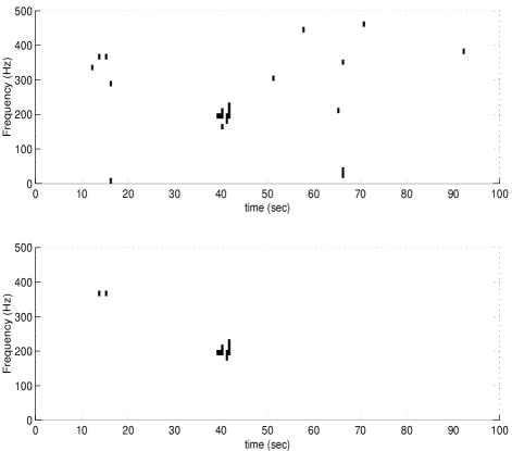
FIG. 2.: Test output for simulated input data constructed by adding a broad band burst of effective duration 1.0 sec, center frequency 200 Hz and bandwidth 200 Hz to stationary white Gaussian noise. The sampling frequency was chosen to be 1000 Hz. (a) Top: raw image obtained after applying the t-test threshold. (b) Bottom: result of applying the veto to the image in (a). The cluster that occurs earlier in (b) is a false event while the next cluster corresponds to the burst.

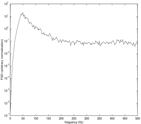
FIG. 3.: PSD for the colored Gaussian noise used in this paper.

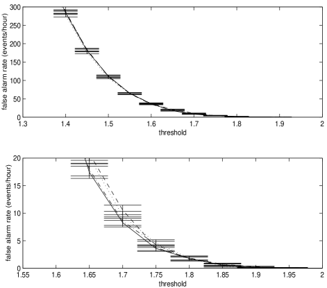
FIG. 4.: False alarm rate as function of threshold for different types of stationary input noise. The sampling frequency of the input is 1000 Hz. Bottom panel: zoomed in view of the top panel. Solid line: white Gaussian noise ($\sigma=1$). Dashed line: white Gaussian noise ($\sigma=10$). Dotted line: white exponential noise ($\sigma=1$). Dash-dotted line: colored Gaussian noise. The error bars correspond to $1\sigma$ deviations. The test parameters values are $l_{l}=0.5$ sec, $l_{s}=0.064$ sec and $\epsilon=3$.

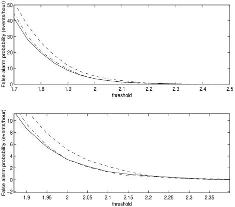
FIG. 5.: False alarm rate as function of threshold for different types of stationary input noise. The sampling frequency of the input is $1000$ Hz. Bottom panel: zoomed in view of the top panel. Solid line: white Gaussian noise ($\sigma=10$). Dashed line: white exponential noise ($\sigma=1.0$). Dash-dotted line: colored Gaussian noise. The test parameters values are $l_{l}=1.25$ sec, $l_{s}=0.064$ sec and $\epsilon=3$.

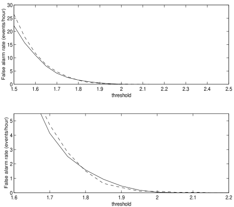
FIG. 6.: False alarm rate as function of threshold for different types of stationary input noise. The sampling frequency of the input is 40 Hz. Bottom panel: zoomed in view of the top panel. Solid line: white Gaussian white noise with ($\sigma=10$). Dashed line: white exponential noise ($\sigma=1.0$). The test parameters values are $l_{l}=1.0$ sec, $l_{s}=0.1$ sec and $\epsilon=3$.

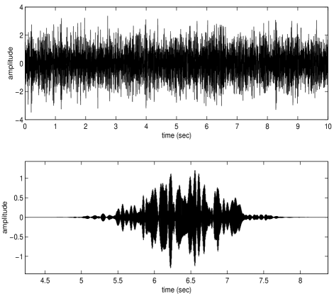
FIG. 7.: Sample realizations a narrow band burst of type (1) and the corresponding input data. Top panel: data obtained by adding a burst to stationary colored Gaussian noise. Bottom: the burst waveform. Here, the peak amplitude of the burst is $1.3\sigma$.

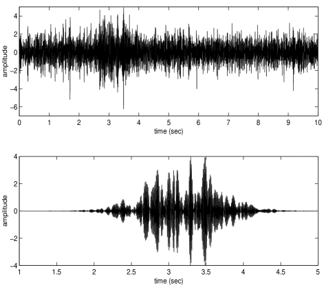
FIG. 8.: Sample realizations of a narrow band burst of type (2) and the corresponding input data. Top panel: data obtained by adding a burst to stationary colored Gaussian noise. Bottom panel: the burst waveform. Here, the peak amplitude of the burst is $4.0\sigma$.

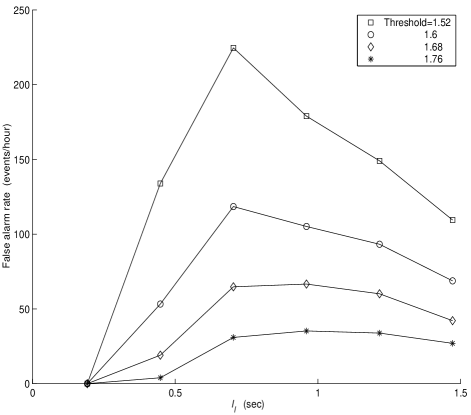
FIG. 9.: Effect of $l_{l}$ ( $l_{s}$ and $\epsilon$ held fixed) on false alarm rate. The stationary noise used was white Gaussian noise ($\sigma=10.0$).

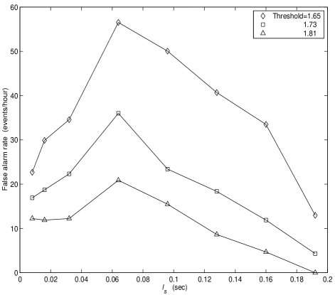
FIG. 10.: Effect of $l_{s}$ ($l_{l}$ and $\epsilon$ held fixed) on the false alarm rate. The stationary noise used was white Gaussian noise ($\sigma=10.0$).

FIG. 11.: Effect of $\epsilon$ on (a) false alarm rate (top) and (b) detection probability (bottom). $l_{l}=0.5$ sec and $l_{s}=0.064$ sec for both (a) and (b). The stationary background noise used was white Gaussian ($\sigma=10$) for (a) and colored Gaussian for (b). In (b), the sudden drop in detection probability occurs, as expected, when the burst duration (chosen to be $2l_{l}$) becomes comparable to $(\epsilon-1)l_{l}$ (which is the actual gap). The total duration of simulated data for (a) was 6.94 hours while the number of trials used for (b) was 800.

FIG. 12.: The effect of burst duration on detection probability. The test parameters were fixed at $l_{l}=0.5$ sec, $l_{s}=0.064$ sec and $\epsilon=5$. The burst peak amplitude for the type (1) bursts ($f_{c}=200$ Hz) was $1.6\sigma$ while it was $4.7\sigma$ for the type (2) bursts ($f_{c}=100$ Hz). The false alarm rate was fixed at 1 false event/hour.

FIG. 13.: Nearest neighbors (gray) of a pixel (brick-wall pattern). The gray pixels which touch the central pixel are its contacting nearest neighbors while the two that do not are its non-contacting nearest neighbors. ($\epsilon=3$ here.)

REFERENCES

- [1] e-mail : mohanty@gravity.phys.psu.edu
- [2] A. Abramovici et al., Science 256, 325 (1992); (http://www.ligo.caltech.edu)
- [3] B. Caron et al., Nucl. Phys. B (Proc. Suppl.) 54 B, 167 (1997).
- [4] K. Danzmann et al., in Gravitational Wave Experiments, edited by E. Coccia, G. Pizzella and F. Ronga (World Scientific, 1997).
- [5] K. Kuroda, in Gravitational waves : Sources and Detectors, edited by I. Ciufolini and F. Fidecaro (World Scientific, 1997).
- [6] D. Sigg, P. Fritschel, LIGO technical document LIGO-T980004-00-D, 1998 (unpublished).
- [7] S. Anderson et al., LIGO technical document LIGO-P990020-00-E, 1999 (unpublished).
- [8] B. Allen et al., Phys. Rev. Lett. 83, 0031-9007 (1999).
- [9] N. Arnaud, F. Cavalier, M. Davier, P. Hello, Phys. Rev. D 59, 082002 (1999).
- [10] E . E. Flanagan, S. A. Hughes, Phys. Rev. D 57, 4535 (1998).
- [11] J. W. Goodman, Statistical Optics (John Wiley, New York, 1985).
- [12] A. Stuart, J. K. Ord, Kendall’s Advanced Theory of Statistics (Edward Arnold, 1991), Vol. 2, fifth edition.
- [13] G. W. Snedecor, W. G. Cochran, Statistical methods (Iowa State Univ. Press, 1980), seventh edition .
- [14] B. Sinha, A. Rukhin, M. Ahsanullah (eds.), Applied Change Point Problems in Statistics (Nova Science Publishers, 1995).
- [15] M. B. Priestley, J. Roy. Statist. Soc. Ser. B, 27, 204 (1965).
- [16] B. Allen, GRASP : Users Manual, University of Wisconsin, Miwaukee, 1997, Version 1.5.0, p. 81.
- [17] B. E. Brodsky, B. S. Darkhovsky, Nonparametric Methods in Change-Point Problems (Kluwer Academic Publishers, 1993).
- [18] N. L. Johnson, S. Kotz, N. Balakrishnan, Continuous Univariate Distributions (Wiley & Sons, New York, 1994).
- [19] R. C. Geary, Supp. Journal of Royal Statistical Society, 3, 178 (1936).
- [20] C. W. Helstrom, Statistical Theory of Signal Detection (Pergamon Press, 1968), 2nd Ed.
- [21] An exponential probability density function is given by , where is both the mean and standard deviation of . For instance, the sum of the squares of two independent and identically distributed Gaussian random variables is distributed as an exponential.
- [22] L. S. Finn, D. F. Chernoff, Phys. Rev. D 47, 2198 (1993).
- [23] G. V. Pallotino, G. Pizzella, in The Detection of Gravitational Waves, edited by D. G. Blair (Cambridge University Press, 1991).
- [24] E. S. Page, Biometrika 41, 100 (1954).
- [25] S. Hayking, Adaptive filter theory (Prentice Hall, 1996), third edition.
- [26] http://www.mathworks.com
- [27] http://www.wolfram.com