The fate of Reissner-Nortström black hole in the Einstein-Yang-Mills-Higgs system

Abstract

We study about an evaporating process of black holes in SO(3) Einstein-Yang-Mills-Higgs system. We consider a massless scalar field which couple neither with the Yang-Mills field nor with the Higgs field surrounding the black hole. We discuss differences in evaporating rate between a monopole black hole and a Reissner-Nortström (RN) black hole. Since a RN black hole is unstable below the point at which a monopole black hole emerges, it will transit into a monopole black hole as suggested via a catastrophe theory. We then conjecture the following: Starting from a Reissner-Nortström black hole, the mass decreases via the Hawking radiation and the black hole will reach a critical point. Then it transits to a monopole black hole. We find that the evaporation rate will increase continuously or discontinuously according to the type of phase transition, that is either second order or first order, respectively. After its transition, the evaporation will never stop because the Hawking temperature of a monopole black hole diverges at the zero horizon limit and overcomes the decrease of the transmission amplitude $\Gamma$.

I Introduction

For many years, there have been various efforts to find a theory of “everything”. One of the candidates is the superstring theory which has been the cause of much attention for last several years in the context of black hole thermodynamics. Since the discovery of black hole radiation by Hawking[1] which is now called Hawking radiation, black hole thermodynamics takes its position beyond the analogy of ordinary thermodynamics.

But Hawking radiation is a semiclassical phenomenon which means that space-time itself is treated classically and matter field is quantized around its metric. Although the gravitational field should also be quantized when the curvature radius gets as small as the Plancknian length ($l_{p}\sim 1.6\times 10^{-33}cm$), usually we ignore it and estimate the effect of Hawking radiation, e.g., as $\gamma$-ray sources of the early universe[2]. When we consider the evaporation process of a Schwarzschild black hole, the Hawking temperature arises monotonically and Hawking radiation does not stop, so classical physics will break down and quantum gravity effects should be considered. This is a serious unsolved problem which will be a key to quantum gravity. But if we think about Hawking radiation of a Reissner-Nortström (RN) black hole in the Einstein-Maxwell (EM) system, its fate is completely different because its temperature will go down and the evaporation process will cease, if we assume that the electric charge is conserved.

Such fates and related things have been investigated by many authors. But as for the black holes with non-Abelian hair[3, 4, 5, 6, 7, 8, 9], they have not been much investigated because their black hole solutions themselves are only obtained numerically, which takes much work compared with black holes analytically obtained. Another cause is perhaps due to their instability in which case the evaporation process need not be considered. But for some types of non-Abelian black holes, there exist stable solutions. Particularly, a monopole black hole which is found in SO(3) Einstein-Yang-Mill-Higgs (EYMH) system is important in the context of Hawking radiation[10, 11, 12, 13]. In the EYMH system, if we consider the evaporation process of the RN black hole, its fate will be rather different from that in the EM system, since it may experience a phase transition and become a monopole black hole. In contrary to the RN black hole, when a monopole black hole evaporates, the Hawking temperature rises monotonically like the Schwarzschild black hole and it may have the possibility to become a regular monopole. If this is the case, it may shed new light on the problem of the remnant of Hawking radiation. So we need to study its evaporation.

This paper is organized as follows. In Sec. II, we introduce basic Ansätze and the field equations in the EYMH system. In Sec. III, we briefly review black holes in the EYMH system and their thermodynamical properties. In Sec. IV, we investigate the evaporating features of RN and monopole black holes in the EYMH system. In Sec. V, we make some concluding remarks and mention some discussion. Throughout this paper we use units $c=\hbar=1$. Notations and definitions such as Christoffel symbols and curvature follow Misner-Thorne-Wheeler[14].

II Basic equations

We consider black hole spacetime in the SO(3) EYMH model as

$$S=\int d^{4}x\sqrt{-g}\left[\frac{R}{2\kappa^{2}}+L_{m}\right],$$ (1)

where $\kappa^{2}\equiv 8\pi G$ with $G$ being Newton’s gravitational constant. $L_{m}$ is the Lagrangian density of matter fields which are written as

$$L_{m}=-\frac{1}{4}F^{a}_{\mu\nu}F^{a\mu\nu}-\frac{1}{2}(D_{\mu}\Phi^{a})(D^{\mu}\Phi^{a})-\frac{\lambda}{4}(\Phi^{a}\Phi^{a}-v^{2})^{2}\ .$$ (2)

$F^{a}_{\mu\nu}$ is the field strength of SU(2) YM field and is expressed by its potential $A^{a}_{\mu}$ as

$$F^{a}_{\mu\nu}=\partial_{\mu}A^{a}_{\mu}-\partial_{\nu}A^{a}_{\nu}+e\epsilon^{abc}A^{b}_{\mu}A^{c}_{\nu},$$ (3)

with a gauge coupling constant $e$. $\Phi^{a}$ is a real triplet Higgs field and $D_{\mu}$ is the covariant derivative:

$$D_{\mu}\Phi^{a}=\partial_{\mu}\Phi^{a}+e\epsilon^{abc}A^{b}_{\mu}\Phi^{c}.$$ (4)

The theoretical parameters $v$ and $\lambda$ are a vacuum expectation value and a self-coupling constant of a Higgs field, respectively. To obtain black hole solutions, we assume that a space-time is static and spherically symmetric, in which case the metric is written as

$$ds^{2}=-f(r)e^{-2\delta(r)}dt^{2}+f(r)^{-1}dr^{2}+r^{2}d\Omega^{2},$$ (5)

where $f(r)\equiv 1-2Gm(r)/r$. For the matter fields, we adopt the hedgehog ansatz given by

$$\Phi^{a}=v\mbox{\boldmath$r$}^{a}h(r),$$ (6)

$$A^{a}_{0}=0,$$ (7)

$$A^{a}_{\mu}=\omega^{c}_{\mu}\epsilon^{acb}\mbox{\boldmath$r$}^{b}\frac{1-w(r)}{er},\;\;\;\;\;(\mu=1,2,3),$$ (8)

where $\mbox{\boldmath$r$}^{a}$ and $\omega^{c}_{\mu}$ are a unit radial vector in the internal space and a triad, respectively.

Variation of the action (1) with the matter Lagrangian (2) leads to the field equations

$$\frac{d\delta}{d\tilde{r}}=-8\pi\tilde{r}\tilde{v}^{2}\tilde{K},$$ (9)

$$\frac{d\tilde{m}}{d\tilde{r}}=4\pi\tilde{r}^{2}\tilde{v}^{2}\left[f\tilde{K}+\tilde{U}\right],$$ (10)

$$\frac{d^{2}w}{d\tilde{r}^{2}}=\frac{1}{f}\left[\frac{1}{2}\frac{\partial\tilde{U}}{\partial w}+8\pi\tilde{r}\tilde{v}^{2}\tilde{U}\frac{dw}{d\tilde{r}}-\frac{2\tilde{m}}{\tilde{r}^{2}}\frac{dw}{d\tilde{r}}\right],$$ (11)

$$\frac{d^{2}h}{d\tilde{r}^{2}}=-\frac{dh}{d\tilde{r}}\frac{1}{\tilde{r}}+\frac{1}{f}\left[\frac{\partial\tilde{U}}{\partial h}+8\pi\tilde{r}\tilde{v}^{2}\tilde{U}\frac{dh}{d\tilde{r}}-\frac{1}{\tilde{r}}\frac{dh}{d\tilde{r}}\right],$$ (12)

where

$$\tilde{U}\equiv\frac{(1-w^{2})^{2}}{2\tilde{r}^{4}}+\left(\frac{wh}{\tilde{r}}\right)^{2}+\frac{\tilde{\lambda}}{4}(h^{2}-1)^{2},$$ (13)

$$\tilde{K}\equiv\frac{1}{\tilde{r}^{2}}\left(\frac{dw}{d\tilde{r}}\right)^{2}+\frac{1}{2}\left(\frac{dh}{d\tilde{r}}\right)^{2}.$$ (14)

We have introduced the following dimensionless variables:

$$\tilde{r}=evr,\ \ \tilde{m}=Gevm,\ \$$ (15)

and dimensionless parameters:

$$\tilde{v}=v\sqrt{G},\;\;\tilde{\lambda}=\lambda/e^{2}.$$ (16)

Although the solution exists when $v\leq M_{Pl}$, where $M_{Pl}$ is Planck mass, it can be described by a classical field configuration in the limit of a weak gauge coupling constant $e$, because its Compton wavelength $\sim e/v$ is much smaller than the radius of the classical monopole solution ($\sim 1/ev$) in this case. Moreover, since the energy density is $\sim e^{2}v^{4}\ll M_{Pl}^{4}$, we can treat this classically if we ignore the effect of gravity. The boundary conditions at spatial infinity are

$$m(\infty)=M<\infty,\ \ \delta(\infty)=0,\ \ h(\infty)=1,\ \ w(\infty)=0.$$ (17)

These conditions imply that space-time approaches a flat Minkowski space with a charged object.

To obtain a black hole solution, we assume the existence of a regular event horizon at $r=r_{H}$. So the metric components are

$$m_{H}\equiv m(r_{H})=\frac{r_{H}}{2G},\ \ \delta_{H}\equiv\delta(r_{H})<\infty.$$ (18)

We also require that no singularity exists outside the horizon, i.e.,

$$m(r)<\frac{r}{2G}\ ~{}~{}~{}~{}~{}{\rm for}~{}~{}~{}r>r_{H}\ .$$ (19)

For the matter fields, the square brackets in Eqs. (11)-(12) must vanish at the horizon. Hence we find that

$$\left.\frac{dw}{d\tilde{r}}\right|_{\tilde{r}=\tilde{r}_{H}}=\frac{w_{H}}{F}\left(1-w^{2}_{H}-h^{2}_{H}\tilde{r}^{2}_{H}\right)$$ (20)

$$\left.\frac{dh}{d\tilde{r}}\right|_{\tilde{r}=\tilde{r}_{H}}=-\frac{h_{H}}{F}\left[2w^{2}_{H}+\tilde{\lambda}\tilde{r}^{2}_{H}(h^{2}_{H}-1)\right]$$ (21)

where

$$F = 2\pi\tilde{v}^{2}\tilde{r}_{H}\left[2\tilde{r}^{-2}_{H}(1-w^{2}_{H})^{2}+4w^{2}_{H}h^{2}_{H}+\tilde{\lambda}\tilde{r}^{2}_{H}(h^{2}_{H}-1)^{2}\right]$$ (23)

$$-\tilde{r}_{H}.$$

Hence, we should determine the values of $w_{H}$, and $h_{H}$ iteratively so that the boundary conditions at infinity are fulfilled.

Non-trivial solution does not necessarily exist for given physical parameters. However, for arbitrary values of $\tilde{v}$ and $\tilde{\lambda}$, there exists an RN black hole solution such as

$$w\equiv 0,\ h\equiv 1,\ \delta\equiv 0,\ \tilde{m}(\tilde{r})\equiv\tilde{M}-\frac{2\pi\tilde{v}^{2}}{\tilde{r}}\ .$$ (24)

$\tilde{M}$ is the gravitational mass at spatial infinity and $\tilde{Q}\equiv 2\sqrt{\pi}\tilde{v}$ is the magnetic charge of the black hole. The radius of the event horizon of the RN black hole is constrained to be $\tilde{r}_{H}\geq\tilde{Q}$. The equality implies an extreme solution.

Around these black holes, we consider a neutral and massless scalar field which does not couple with the matter fields, i.e., either Yang-Mills nor Higgs fields. This is described by the Klein-Gordon equation as

$$\Phi_{,\mu}^{\ ;\mu}=0.$$ (25)

The energy emission rate of Hawking radiation is given by

$$\frac{dM}{dt}=-\frac{1}{2\pi}\sum_{l=0}^{\infty}(2l+1)\int_{0}^{\infty}\frac{\Gamma(\omega)\omega}{e^{\omega/T_{H}}-1}d\omega,$$ (26)

where $l$ and $\Gamma(\omega)$ are the angular momentum and the transmission probability in a scattering problem for the scalar field $\Phi$. $\omega$ and $T_{H}$ are the energy of the particle and the Hawking temperature respectively. We define as $\Xi\equiv-dM/dt$.

The Klein-Gordon equation (25) can be made separable, and we should only solve the radial equation

$$\frac{d^{2}\chi}{d\tilde{r}^{\ast 2}}+\chi\left[\tilde{\omega}^{2}-\tilde{V}^{2}\right]=0,$$ (27)

where

$$\tilde{V}^{2} \equiv \frac{f}{\tilde{r}e^{2\delta}}\left\{\frac{l(l+1)}{\tilde{r}}-f\delta^{\prime}+\frac{2(\tilde{m}-\tilde{m}^{\prime}\tilde{r})}{\tilde{r}^{2}}\right\},$$ (28)

$$\frac{d\tilde{r}}{d\tilde{r}^{\ast}} \equiv fe^{-\delta},$$ (29)

where ^′ denotes $d/d\tilde{r}$ and $\chi$ is only the function of $r$. We need the normalization as $\tilde{\omega}=\omega/ev$, $\tilde{V}=V/ev$. The transmission probability $\Gamma$ can be calculated by solving the radial equation numerically under the boundary condition

$$\chi\rightarrow Ae^{-i\omega r^{\ast}}+Be^{i\omega r^{\ast}}\ \ (r^{\ast}\rightarrow\infty),$$ (30)

$$\chi\rightarrow e^{-i\omega r^{\ast}}\ \ (r^{\ast}\rightarrow-\infty),$$ (31)

where $\Gamma$ is given as $1/|A|^{2}$. In our case, if we obtained the black hole solution, i.e., the shooting parameters $w_{H}$ and $h_{H}$, we should integrate (27) and (9)-(12) simultaneously.

III Black Holes in the Einstein-Yang-Mills-Higgs system

In this section, we briefly explain about black holes in the EYMH system, particularly about thermodynamical properties. We show the relation between horizon radius $\tilde{r}_{H}$ and gravitational mass $\tilde{M}$ in Fig. 1(a). We denote RN and monopole black holes by a dotted line and a solid line, respectively. We chose as $\tilde{\lambda}=\tilde{v}=0.1$. In this figure, we can see that RN and monopole black holes emerge at the point $B$ which does not change even if we change $\tilde{\lambda}$. On the contrary, if we change $\tilde{v}$, the point $B$ moves and disappears for large $\tilde{v}$ (i,e., they do not emerge.). The precise are shown in [10]. We only consider the parameter region where the point $B$ exists, because it is shown in [11] that the RN black hole becomes unstable via linear perturbation below the point $B$ and later analysis showed that the RN black hole may transits to the monopole black hole only in this case.

Before denoting the stability of monopole black hole, we show the magnification of Fig. 1 (a) around the point $B$ in Fig. 1 (b). We find a cusp structure at the point $A$ which exists for $\tilde{\lambda}<\tilde{\lambda}_{crit}$. $\tilde{\lambda}_{crit}$ slowly depends on $\tilde{v}$. We can understand them via swallow tail catastrophe[13]. We can see in Fig. 1 (b) that for some mass range which corresponds to $B$ to $A$, there appear three types of solutions (stable RN black hole, stable and unstable monopole black holes) which suggests the violation of weak no hair conjecture. By contrast, for $\lambda>\lambda_{crit}$, a cusp structure never appears and the monopole black hole solution merges with the RN black hole at the point $B$. From the analysis in [13], we can summerize the stability of black holes as follows:

(i) As for the RN black hole, the stability changes at the point $B$. It is stable or unstable according to be above or below the point $B$.

(ii) As for the monopole black hole, when $\tilde{\lambda}<\tilde{\lambda}_{crit}$, it is unstable along the curve from $A$ to $B$, otherwise it is stable. When $\tilde{\lambda}>\tilde{\lambda}_{crit}$, it is always stable.

We also show the inverse temperature $1/T_{H}$ in terms of the gravitational mass $M/(M_{pl}^{2}/ev)$ in Fig. 1(c). Assuming the conservation of charge and starting with the RN black hole, the point $B$ is a key to the fate of the black hole. Because if we consider the RN black hole in the EM system, the RN black hole is always stable and the evaporation will cease at the extreme limit because the temperature vanishes there. While if we have the RN black hole in the EYMH system, the RN black hole becomes unstable below the critical point $B$ and will change to a monopole black hole by either second- or first- order transition according to $\lambda>\lambda_{crit}$ or $\lambda<\lambda_{crit}$. After this transition, because the temperature diverges to infinity at the $r_{H}\rightarrow 0$ limit, so we may not stop evaporating a monopole black hole and find that one of the candidates for the remnant is a self-gravitating monopole. We show the diagram for $\tilde{\lambda}=\tilde{v}=0.1$. But the results are qualitatively same for other parameters (see Fig. 9 (a) in [13]).

The criterion stable or unstable is based on casastrophe which coincide with the analysis via linear perturbation. So if we think evaporation process and time evolution of them, the results may change. But it may be laborious to calculate such evolution, here we consider mainly about transmission amplitude of a scalar field assuming black holes as a background.

IV Evaporation of Black Holes in the Einstein-Yang-Mills-Higgs system

Even if we assume that the background spacetime is fixed and ignore backreaction, it is not evident to predict the final fate of black holes. Naively speaking, the temperature is the main cause to decide evaporation process. But the transmission amplitude $\Gamma$ may also affect the results. For example, a dilatonic black hole in the EM-dilaton system has different properties via a coupling constant $\alpha$ of the dilaton field to the matter field[15]. If $\alpha>1$, the temperature of the black hole diverges and the effective potential $V^{2}$ grows infinitely high simultaneously at the extreme limit[16]. In this case, it is not evident how to decide whether or not the emission rate diverges. In [17], it turned out that the divergence of the temperature at the extreme limit overcomes that of the effective potential, resulting in a divergence of the emission rate.

In the case of a monopole black hole, it is not even evident whether or not the effective potential diverges at the $r_{H}\rightarrow 0$ limit, because its solution is only obtained numerically. Fig. 2 shows the effective potential $(V/ev)^{2}$ in terms of the radial coordinate for $v/M_{pl}=0.05$, $\lambda/e^{2}=1$ and $r_{H}/(ev)^{-1}=0.1$, $0.3$. Taking the horizon radius as smaller, the potential $V^{2}$ becomes larger and our numerical results suggest that its potential diverges within that limit, so we must analyze the emission rate to decide whether or not the evaporation will stop. Another interesting point is how Hawking radiation changes at the point $B$ in the transition process of an RN black hole to a monopole black hole. Near the point $B$ we can suggest something concrete under some assumptions. For this, we assume the following: (i) The coupling constant $e$ is small enough so that we can treat the gravitational field classically at the point B. (ii) A discharge process does not occur during the evaporation[18]. (iii) The coupling of the matter fields (YM and Higgs fields) to the scalar field even if it exists, the results would not be much affected. The last ansatz may seem to be strong, but it might turn out to be true near the point $B$ because the monopole black hole around there is very close to the RN black hole, which is a vacuum solution. In fact the field strength of YM field for such a monopole black hole is much smaller than that in the other cases.

Before seeing such properties, we show the transmission probability $\Gamma$ of a RN black hole and a monopole black hole in terms of $\omega$ for the horizon radius $r_{H}/(ev)^{-1}=0.55$ and $v/M_{pl}=0.05$, $\lambda/e^{2}=0.1$, $1$ in Fig. 3 (a). We depict only $l=0$, $1$ modes. The RN black hole, monopole black hole with $\lambda/e^{2}=0.1$, monopole black hole with $\lambda/e^{2}=1$ correspond to the dotted lines, the solid lines and the dot-dashed lines, respectively. As we see the dominant contribution for the Hawking radiation is $l=0$, because the contributions of the higher modes are suppressed by the centrifugal barrier. In what follows, we will ignore the contributions from $l\geq 2$. Although $\Gamma$ is the largest for an RN black hole, these are almost indistinguishable. So, when evaluating the value of the emission rate of a monopole black hole, we may conclude that $\Gamma$ may not be the main origin of the difference from that of the RN black hole. However, for a monopole black hole with a smaller horizon radius, its difference from an RN black hole becomes clear. Fig. 3 (b) shows the same diagram in Fig. 3 (a) with the same parameters $v$ and $\lambda$ but with a smaller horizon radius $r_{H}=0.3/ev$. We can see the difference clearly. It is because the size of non-trivial structure becomes larger compared with the horizon radius for the monopole black hole of smaller horizon. We also show the examples of the radiation spectrum $-d^{2}M/dtd\omega$ in terms of $\omega$ in Fig. 4 (a), (b). The parameters correspond to Fig. 3 (a), (b). One can see the reason why we can ignore the contribution for $l\geq 2$. Actually, the difference caused by it is below $1\%$ from one of our calculation.

We return to the first concern, i.e., what happens when the horizon radius changes via Hawking radiation. In Fig. 5 (a), we show the emission rate $\Xi$ in terms of the gravitational mass $M$ of an RN black hole and a monopole black hole for $v/M_{pl}=0.05$, $\lambda/e^{2}=1$. The difference between an RN black hole and a monopole black hole may be caused by the Hawking temperature $T_{H}$, because the emission rate $\propto T_{H}^{4}$. In Fig. 5 (b), we show the emission rate $\Xi$ in terms of the horizon radius $\tilde{r}_{H}$ for the same parameters in Fig. 5 (a). This diagram strongly suggest that the evaporation will not stop even at the $r_{H}\to 0$ limit. This resembles the situation of the dilatonic black hole at the extremal limit, i.e., whether or not evaporation stop depends only on $T_{H}$[17]. Thus whenever we think black hole space-times as background, the transmission amplitude does not change the scenario estimating from the temperature.

We estimate the time scale of the evaporation using $T_{time}\equiv M/\Xi$ as the indicator, and show this time scale in terms of the gravitational mass $M$ in Fig. 6 for the same solutions in Fig. 5 in the CGS units. Near the bifurcation point $B$, $T_{time}\sim 10^{-37}/e^{3}\ second$, and below the bifurcation point, the time evolution of the monopole black hole is completely different from that of an RN black hole.

Next, we study the evaporation rate near the bifurcation point when either the first or second order transition to the monopole black hole occurs. In Fig. 7, we show the emission rate $\Xi$ in terms of the gravitational mass $M$ of RN and monopole black holes for $v=0.05M_{pl}$, $\lambda/e^{2}=0.1$, $0.2$, $0.3$, $0.4$, $1$ near the bifurcation point. The curves from $B$ to $A$ correspond to the emission rate of the unstable branch. In the case that the transition is first order, the emission rate will also change discontinuously as shown by an arrow in Fig. 7.

It may be interesting to ask in which direction the RN black hole jumps to the monopole black hole or how much black hole entropy (or radius of event horizon) will increase after the phase transition. In order to analyze this problem properly, we have to include a back reaction effect of Hawking radiation, which is very difficult and has not yet been solved. However, we may find some constraints through the following considerations. Because the RN black hole emits particles, it will lose some of the gravitational mass. But, whether the horizon radius increases or not may depend on two time scales, i.e. the evaporation time and the transition time. If we apply the catastrophe theory, the entropy of the black hole will increase and the horizon radius will increase. But this analysis is based on the assumption that the change of black hole states can be treated adiabatically. Since the coupling constant $e$ is so small that each state can be described by a quasi-stationary solution, we may expect that the horizon radius will increase after the transition.

We also confirm that an other choice of values of $v$ and $\lambda$ does not provide any serious difference in the evaporation process. In Fig. 8, we show one of the interesting cases ($\lambda/e^{2}=0.1$ and $v=0.2M_{pl}$) where the bifurcation point $B$ is very near the extreme RN solution. In this case, this diagram suggests that the RN black hole first almost ceases the evaporation process and becomes close to the extreme one, and then it transits to a monopole black hole and will start to evaporate again. In other parameters, these diagrams are basically similar to the above cases:

(i) The emission rate diverges at the $\tilde{r}_{H}\to 0$ limit.

(ii) Near the bifurcation point $B$, the emission rate changes continuously or discontinuously according to $\tilde{\lambda}$ is above or below $\tilde{\lambda}_{crit}$.

V Conclusion and discussion

We have considered an evaporation process of the RN and monopole black holes in the EYMH system. We have analyzed a real massless scalar field which couple to neither the NA field nor the Higgs field. We may suggest how RN and monopole black holes evolve through an evaporation process in the EYMH system. We have the following results.

(i) We investigated the evaporation process of an RN black hole, in particular, near the bifurcation point where this merges with a branch of monopole black holes. Since the RN black hole becomes unstable there, we expect that it transits into a monopole black hole. This transition will be first- or second-order according to whether $\lambda$ is smaller than some critical value $\lambda_{crit}$ or not. We show that the evaporation rate changes continuously or discontinuously depending on whether the transition which occurs is second- or first-order. Our results suggest that the Hawking radiation near the bifurcation point is determined only by the temperature of the black hole. We can understand this as follows. Because in particular, around this region, we find little difference in the transmission probability between a monopole black hole and an RN black hole.

(ii) When the horizon radius becomes small, the transmission probability of a monopole black hole becomes small compared with that of an RN black hole. Though it can not stop evaporating in our analysis because the increase of temperature of a monopole black hole at the $r_{H}\rightarrow 0$ limit, quantum effects of gravity may cause a serious effect on it and would overcomes the decrease of $\Gamma$.

We finally remark on some subjects which we leave to the future. When we consider the fate of an RN black hole via Hawking radiation, we may take into account the effects of charge loss if it is to be expected, and have to include a coupling to the YM field or Higgs field before we consider the effects of quantum gravity. The second is the concern with the critical behavior[19]. There are several works about it in the EYM or Einstein-Skyrme systems[20, 21], in which the Schwarzschild black hole is the most stable one. But in the EYMH system, since a monopole black hole becomes more stable than the RN black hole below a certain critical mass, it would be interesting to study the critical behavior in the EYMH system. Finally, it may be more interesting to look for the “real” critical behaviour in our present phase transition via Hawking evaporation. Those are under investigation.

ACKOWLEDGEMENTS

Special thanks to J. Koga, T. Torii and T. Tachizawa for useful discussions. T. T is thankful for financial support from the JSPS. This work was supported partially by a JSPS Grant-in-Aid (No. 106613), and by the Waseda University Grant for Special Research Projects.

FIG. 1.: (a) the gravitational mass $M/(M_{pl}^{2}/ev)$ and the horizon radius $r_{H}/(ev)^{-1}$ relation and (b) its magnification diagram near the point $B$ and (b) the inverse Hawking temperature $(T_{H}/eM_{pl}^{2})^{-1}$ in terms of the gravitational mass $M/(M_{pl}^{2}/ev)$ of the monopole black hole with $\lambda/e^{2}=0.1$ (solid lines) and of the RN black hole (dotted lines). We choose $v/M_{pl}=0.1$ in these diagrams. At the point $B$, the RN black hole becomes unstable and change to monopole black hole. This process is first or second order correspond to $\lambda$ is larger than $\lambda_{crit}$ or not. Fig. (c) shows that temperature of the monopole black hole diverges at the $\tilde{r}_{H}\to 0$ limit like the Schwarzschild one. Though we showed the one example, which is irrelevant to the results (see Fig. 9 (a) in [13].).

FIG. 2.: We show the potential $V^{2}/(ev)^{2}$ in terms of the radial coordinate with $\lambda/e^{2}=1$, $v/M_{pl}=0.05$ and $r_{H}/(ev)^{-1}=0.1$, $0.3$ for $l=0$ mode. It shows that when horizon radius $r_{H}$ becomes small, potential barrier becomes large. It seems that if we take $r_{H}\rightarrow 0$, potential barrier diverges.

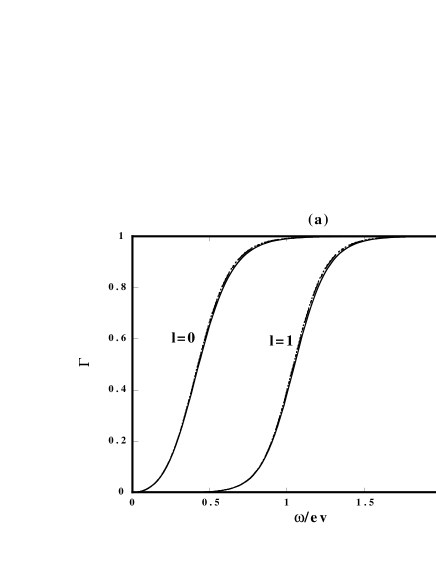
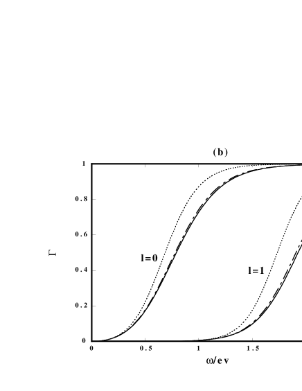
FIG. 3.: Energy dependence of the transmission amplitude $\Gamma$ for monopole black holes with $\lambda/e^{2}=0.1$ (solid lines) and $\lambda/e^{2}=1$ (dot-dashed lines) and of RN black holes (dotted lines) for $l=0$, $1$ mode which make the main contributions to the Hawking radiation. We choose $v/M_{pl}=0.05$ in these diagrams and (a) $r_{H}/(ev)^{-1}=0.55$ (b) $r_{H}/(ev)^{-1}=0.3$. Though the RN black hole has the largest $\Gamma$ among them, these are almost indistinguishable in (a). But when horizon radius becomes small, their difference becomes large because YM field and Higgs field outside the horizon becomes large and contribute to the black hole structure.

FIG. 4.: Energy spectrum of the $-d^{2}m/dtd\omega$ for black holes corresponding to Fig. 3 (a), (b). They shows that why we can neglect the contribution from $l\geq 2$.

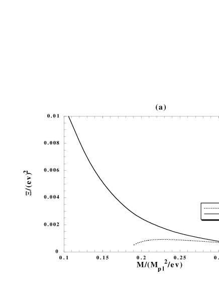
FIG. 5.: The emission rate $\Xi/ev$ (a) in terms of the gravitational mass $M/(M_{pl}^{2}/ev)$ (b) in terms of the horizon radius $r_{H}/(ev)^{-1}$ for RN and monopole black holes for $v/M_{pl}=0.05$, $\lambda/e^{2}=1$. If we assume the charge is conserved, though the RN black hole will stop evaporating at the extreme limit, monopole black hole does not stop evaporating as in the Schwarzschild black hole. If we consider the effects of quantum gravity, the results near $r_{H}\sim l_{p}$ may be changed.

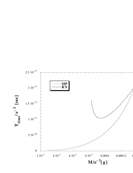
FIG. 6.: The evaporation time scale $T_{time}$ in terms of the gravitational mass $M$ in the CGS units for the same solutions in Fig. 5.

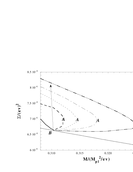
FIG. 7.: The emission rate $\Xi/ev$ in terms of the gravitational mass $M/(M_{pl}^{2}/ev)$ for RN and monopole black holes for $v/M_{pl}=0.05$, $\lambda/e^{2}=0.1$, $0.2$, $0.3$, $0.4$, $1$ near the bifurcation point $B$. The lines from $B$ to $A$ correspond to the emission rate of the monopole black hole which is thought to be unstable. So when the transition from the RN black hole to the monopole black hole occurs, emission rate will raise above the points $A$.

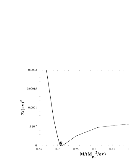
FIG. 8.: The emission rate $\Xi/ev$ in terms of the gravitational mass $M/(M_{pl}^{2}/ev)$ for $v/M_{pl}=0.2$. We chose $\lambda/e^{2}=0.1$. In this figure, we considered the situation bifurcation point almost coincide with extreme RN black hole. This figure shows that evaporation feature drastically changes near the extreme point because of the transition into the monopole black hole.

REFERENCES

- [1] S. W. Hawking, Nature 248, 30 (1974); Commun. Math. Phys. 43, 199 (1975).
- [2] D. N. Page and S. W. Hawking, Astrophys. J. 206, 1 (1976).
- [3] As a review paper see K. Maeda, Journal of the Korean Phys. Soc. 28, S468, (1995), and M. S. Volkov and D. V. Gal’tsov, Phys. Rept. 319, 1 (1999).
- [4] M. S. Volkov and D. V. Galt’sov, Pis’ma Zh. Eksp. Theor. Fiz. 50, 312 (1989); P. Bizon, Phys. Rev. Lett. 64, 2844 (1990); H. P. Künzle and A. K. Masoud-ul-Alam, J. Math. Phys. 31, 928 (1990).
- [5] K. Maeda, T. Tachizawa, T. Torii and T. Maki, Phys. Rev. Lett. 72, 450 (1994); T. Torii, K. Maeda and T. Tachizawa, Phys. Rev. D. 51, 1510 (1995).
- [6] S. Droz, M. Heusler and N. Straumann, Phys. Lett. B 268, 371 (1991).
- [7] B. R. Greene, S. D. Mathur and C. M. O’Neill, Phys. Rev. D 47, 2242 (1993).
- [8] H. Luckock and I. G. Moss, Phys. Lett. B 176, 341 (1986); H. Luckock, in String theory, quantum cosmology and quantum gravity, integrable and conformal invariant theories, eds. H. de Vega and N. Sanchez, (World Scientific, Singapore, 1986), p. 455.
- [9] T. Torii and K. Maeda, Phys. Rev. D 48, 1643 (1993).
- [10] P. Breitenlohner, P. Forgács and D. Maison, Nucl. Phys. B 383, 357 (1992); ibid. 442, 126 (1995).
- [11] K. -Y. Lee, V. P. Nair and E. Weinberg, Phys. Rev. Lett. 68, 1100 (1992); Phys. Rev. D 45, 2751 (1992); Gen. Relativ. Gravit. 24, 1203 (1992).
- [12] P. C. Aichelberg and P. Bizon, Phys. Rev. D. 48, 607 (1993).
- [13] T. Tachizawa, K. Maeda and T. Torii, Phys. Rev. D. 51, 4054 (1995).
- [14] C. W. Misner, K. S. Thorne and J. A. Wheeler, Gravitation (Freeman, New York 1973).
- [15] G.W. Gibbons and K. Maeda, Nucl. Phys. B 298, 741 (1988).
- [16] We use the same notation as in [17].
- [17] J. Koga and K. Maeda, Phys. Rev. D. 52, 7066 (1995).
- [18] W. T. Zaumen, Nature 247, 530 (1974); G. W. Gibbons, Comm. Math. Phys. 44, 245 (1975).
- [19] M. W. Choptuik, Phys. Rev. Lett. 70, 9 (1993).
- [20] M. W. Choptuik, P. Bizon, and T. Chmaj, Phys. Rev. Lett. 77, 424 (1996). ; M. W. Choptuik, Eric W. Hirschmann, and Robert. L. Marsa, Phys. Rev. D. 60, 124011 (1999).
- [21] P. Bizon and T. Chmaj, Phys. Rev. D. 58, 041501 (1998). ; ibid. Acta. Phys. Polon. B 29, 1071 (1998).
- [22] R. M. Wald, General Relativity (Chicago Press, Chicago and London 1984).