[

Collision of 1.4 $M_{\odot}$ Neutron Stars: Dynamical or Quasi-Equilibrium?

Abstract

Shapiro put forth a conjecture stating that neutron stars in head-on collisions (infalling from infinity) will not collapse to black holes before neutrino cooling, independent of the mass of the neutron stars. In a previous paper we carried out a numerical simulation showing a counter example based on 1.4 $M_{\odot}$ neutron stars, and provided an analysis explaining why Shapiro’s argument was not applicable for this case.

A recent paper by Shapiro put forth an argument suggesting that numerical simulations of the 1.4 $M_{\odot}$ collisions could not disprove the conjecture with the accuracy that is presently attainable. We show in this paper that this argument is not applicable for the same reason that the Shapiro conjecture is not applicable to the 1.4 $M_{\odot}$ neutron star collision, namely, the collision is too dynamical to be treated by quasi-equilibrium arguments.

]

Shapiro in [1] proposed an intriguing conjecture on head-on collisions of neutron stars (NSs) infalling from infinity. It goes as follows: For two stable NSs that are described by a polytropic equation of state (EOS) $P=K\rho^{\Gamma}$ [$K=K(s)$ is a function of the entropy $s$, the polytropic index $\Gamma$ is a constant in space and time], it is conjectured that no prompt collapse can occur for an arbitrary $\Gamma$ and an arbitrary initial $K$, independent of the mass of the neutron stars. The basic argument of [1] is that, with the polytropic EOS, there always exists a stable equilibrium TOV configuration with the same total mass and total energy as the two initially isolated TOV stars. As the mass and energy are conserved to a good extent in the head-on collision process, Ref. [1] concluded that the merged object will be stable until energy is radiated away at a much longer timescale.

In [2], we present a counter example to the conjecture. We carried out a numerical simulation of the head-on collision of two 1.4 $M_{\odot}$ neutron stars, with polytropic index of $2$ and initial polytropic coefficient $K=1.16\times 10^{5}\;\frac{{cm}^{5}}{g\;s^{2}}$, a typical choice used in neutron star collision studies (see e.g., [3] and references therein). We found that a black hole is formed promptly. We also proposed a reason why Shapiro’s argument is not applicable to the 1.4 $M_{\odot}$ case (see below).

Recently Shapiro [4] put forth an argument suggesting that the $1.4M_{\odot}$ simulation in [2] could not possibly have the accuracy needed to determine whether a black hole is formed or not. The argument is again based on stable equilibrium TOV configurations. It is pointed out that in order to determine whether a TOV configuration is on the stable or unstable side of the equilibrium curve near the critical point of stability, one has to determine its total energy to very high accuracy. For the 1.4 $M_{\odot}$ simulation reported in [2], it is estimated that the energy must be calculated to within an accuracy of $0.5\%$ throughout the evolution. It is claimed that such an accuracy is beyond what one can achieve with a 3D code with presently available computing power.

In the following we discuss why the observation in [4], although interesting and potentially important to other numerical studies, is irrelevant to the simulation reported in [2]. In fact, the reason why this argument is irrelevant is the same as why the Shapiro’s argument is not applicable to the 1.4 $M_{\odot}$ case in the first place, as given already in [2].

In [2] we pointed out that there is a hidden assumption in Shapiro’s argument, namely, that the collision process can be approximated by a quasi-equilibrium process, in two related senses: (A) The coalescing matter can be described by one single EOS everywhere [$K(s)$ is a function of time but not space, that is, $s$ is a spatial constant, uniform throughout the object], and further, (B) whether it collapses or not is determined by the hydro-static equilibrium condition, i.e., whether a stable equilibrium TOV configuration exists or not. We pointed out in [2] that this quasi-equilibrium assumption is not self-evident for the head-on collision of the 1.4 $M_{\odot}$ NSs after estimating the various time scales involved. In the following we expand on this question of “dynamical” vs. “quasi-equilibrium”.

For concreteness and for the purpose of establishing one counter example to Shapiro’s conjecture, in both [2] and the present paper we focus on the 1.4 $M_{\odot}$ case, with a specific EOS. We shall not comment, nor make any claim, on any other preliminary simulations or results with a different mass or EOS.

In [2] we found that the quasi-equilibrium assumption was broken in the sense of both (A) and (B) for the 1.4 $M_{\odot}$ case . (A) is violated as the coalesced object does not have time to thermalize before it collapses. Notice that with a strong shock, “thermalization” proceeds much faster than the heat conduction time scale. However the shock front is still not fast enough in its outward propagation; it gets trapped inside the apparent horizon before it can reach a good part of the infalling matter. The polytropic coefficient $K(s)$ is never a spatial constant, nor approximately constant, throughout the coalesced object. This implies that (B) must also be violated: the collision process is so dynamical that although a stable equilibrium state exists (allowed by the energy and mass conservation laws), it is not attained in the collapse process.

One central message of [2] and the present paper is that the head-on collision of 1.4 $M_{\odot}$ NSs is so dynamical that one must not use any notion of quasi-equilibrium, on which both the original Shapiro conjecture and the “accuracy argument” are based.

We have already provided evidence for this dynamical nature of the collision in [2]. To strengthen this message of “dynamical” vs. “quasi-equilibrium”, we focus on one specific aspect in this paper. When the two 1.4 $M_{\odot}$ NSs touch after infalling from infinity, they approach one another at a fraction of the light speed. A strong shock is generated, converting about $90\%$ of the bulk kinetic energy to thermal energy in the post-shock material. However, the rest of the stars (pre-shock) cramp in so rapidly that an apparent horizon quickly forms, trapping everything, including the shock front, inside. In Fig. 1 below, the solid line is the world line of the shock front in the $z$ direction (direction of infall), plotted in coordinate distance and coordinate time. The “*” represents the location of the apparent horizon found in the simulation. The dotted line represents one leg of the backward light cone, starting backward from the apparent horizon. The backward light cone meets the shock front at $t=0.195ms$, which is $0.048ms$ after the two stars first touched. At this point the shock has just barely propagated outward and the material heated up by the shock wave (the post-shock material) makes up only a small fraction of the total amount of matter on this time slice. In terms of the number of baryons, it is less than 5%. (One could consider different time slices, but the basic picture is the same.) We do not expect that such an insignificant fraction of heated material could have much effect on the overall dynamics of the infalling matter, let alone providing the thermal pressure to prevent the collapse as envisioned in the Shapiro conjecture. At later times the shock heated material does make up a bigger fraction of the total mass. However, from the point of intersection of the dashed and solid line at $t=0.195ms$ onward, the shock heated material is causally disconnected with the apparent horizon shown and could not affect its formation. This highlights how far away from thermal and dynamical equilibrium the collision process is.

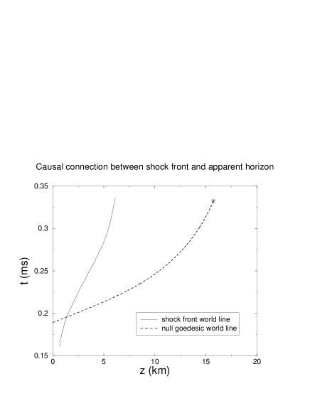
FIG. 1.: The causal relation between the apparent horizon and the shock front is displayed. The point marked by “*” represents the intersection of the apparent horizon with the $+z$ axis (the stars are falling towards one another along the $z$ axis with the center of collision at $z=0$). A null geodesic traveling along the $z$ axis is shown as a dotted line. The solid line represents the world line of the intersection of the shock front on the $+z$ axis. World lines are plotted in coordinate distance vs. coordinate time.

It may be worthwhile to point out that the features of this figure have been quite carefully examined. The position of the AH has been subjected to convergence and stability tests with respect to different boundary conditions and different locations of the outer boundary. The existence of trapped surfaces in the spacetime have been explicitly verified. To confirm the shock propagation speed in the curved spacetime simulation, we have carried out tests in which we extracted the proper density, pressure and velocity of the fluid flow on two sides of the shock at various times in the collision simulation, and set up shock tube tests with the same hydrodynamic conditions in flat space. Such tests are meaningful because of the fact that shock propagation is a local phenomena, and that the flat space shock treatments in our code has been thoroughly tested previously [5]. The details of these tests will be given in a follow up paper.

The main aim of this paper is to contrast the dynamical picture demonstrated in our simulation with the “equilibrium picture” of [1, 4]. In the “equilibrium picture” one envisions that the shock wave bounces a couple of times across the whole coalesced object, heating it up approximately uniformly [so that the polytropic constant $K(s)$ becomes a spatial constant], and the coalesced object can be described by a TOV configuration in equilibrium. Refs. [1] and [4] then analyzed the stability of this “resulting” TOV configuration and concluded that it could not collapse.

The argument of [1] and [4] would be strictly valid if the collision process is in quasi-equilibrium instead of freefall. In Fig. 2, panel (A1) represents two NSs in free fall towards each other. Panel (A2) represents the shock wave heating up the merging stars (with the dark grey area representing the material at higher temperature and hence higher $K$). However, at this point the apparent horizon pops into existence engulfing most of the infalling matter. (A3) represents the black hole finally formed. Fig. 3 represents a thought experiment in which the quasi-equilibrium analysis is valid. Panel (B1) represents two NSs with ropes attached slowly lowered towards one another, with the potential energy extracted and re-deposited back into the stars. This makes the stars gradually heat up, maintaining quasi-equilibrium throughout the process. (To be precise, each fluid element has to be tied and arranged into its quasi-equilibrium position at each point in time.) This is represented in (B2). Darker grey is used to represent the uniformly heated object with the potential energy extracted and redistributed back to it through the ropes. One final equilibrium (hot) TOV star is formed, represented by (B3). The stability of this TOV star is determined by the considerations in Refs. [1] and [4].

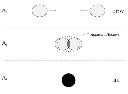
FIG. 2.: The freefall collision of two 1.4 $M_{\odot}$ NSs. In (A1) two NSs are in free fall towards each other. The grey region in panel (A2) represents the material heated by the shock wave. At this point, an apparent horizon forms, engulfing most of the infalling matter. Panel (A3) represents the black hole finally formed.

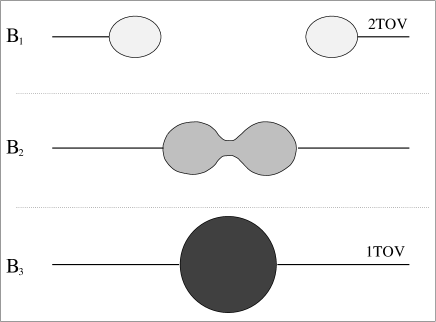
FIG. 3.: The merging of two NSs in quasi-equilibrium. (B1) represents two NSs with ropes attached slowly lowered towards one another, with the potential energy extracted and re-deposited back into the stars. (The fluid elements are tied and arranged into their quasi-equilibrium position throughout the process.) Panel (B2) represents the uniformly heated, merging object with the potential energy extracted and redistributed back to it through the ropes. Panel (B3) represents the final equilibrium TOV star formed. In this quasi-equilibrium scenario the considerations in Refs. [1] and [4] would be strictly applicable.

Fig. 4 schematically represents the configuration space of the coupled Einstein-GRHydro equations. The lower left dot denoted 2TOV represents the state of two TOV configurations infinitely separated. In free fall governed by the coupled Einstein-GRHydro equations, it evolves along the solid line towards the lower right hand dot denoted BH representing the solution of a black hole. The three stages A1, A2 and A3 in Fig. 2 are labeled. The dotted line represents the evolution of the Panels B in Fig. 3 (the Einstein-GRHydro equations with source terms including the ropes): The two TOV stars are tied and lowered towards one another. This leads to the state represented by the dot in upper right hand corner denoted 1TOV. The argument in Ref. [4] amounts to pointing out that should one actually carry out a numerical simulation following this dotted line, one would have to maintain $0.5\%$ accuracy in order to determine whether the 1TOV solution obtained at B3 is stable or not. We see that this accuracy requirement is irrelevant to the head-on collision study: We are not carrying out a simulation along the quasi-equilibrium path (if such a simulation is at all possible).

FIG. 4.: This figure represents the configuration space of the coupled Einstein-GRHydro equations. The lower left dot denoted 2TOV represents the state of two TOV configurations infinitely separated. In free fall governed by the coupled Einstein-GRHydro equations, it evolves along the solid line towards the lower right hand dot denoted BH representing a black hole. The three stages A1, A2 and A3 in Fig. 2 are labeled. The dotted line represents the evolution in quasi-equilibrium depicted in Panels B of Fig. 3: The two TOV stars are tied and lowered towards one another. This leads to the state represented by the dot in upper right hand corner denoted 1TOV.

How accurate do we have to get in following the evolution depicted by the solid line in Fig. 4 before we can be sure that a black hole is actually formed? We do not have an answer to this question presently. The accuracy we achieved can be monitored by the Hamiltonian constraint violation at the point we found the AH (along the z-axis). The Hamiltonian constraint violation is $0.146,0.096,0.062,0.040$ (in units of $16\pi\rho$, with $\rho$ being the maximum rest mass density at that time), for the simulations carried out with grid sizes of $40^{3},96^{3},160^{3},256^{3}$, respectively. The simulations are carried out with only one octant of the grid evolved. (Due to the symmetry of the problem, only one octant of the domain needs to be numerically calculated. The $256^{3}$ simulation corresponds to having about 140 points across the diameter of one star.) We note two points: 1. the formation of a black hole can be obtained by a simulation with rather coarse resolution, and 2. this feature of black hole formation is stable with respect to increasing resolution, i.e., a long time scale convergence test. We emphasize that in numerical studies one must insist that the physical feature one is studying is subjected to, and passes convergence tests. We emphasize that here we are talking about not just the usual short time convergence code test. The convergence tests must be carried out for the specific system of physical interest, and maintained throughout the time of evolution up to the time the physical feature under consideration is extracted: a “long term” convergence test. Together with the consistency tests making sure that the finite difference equations are faithful to the differential equations, one can then invoke the Lax theorem to give oneself a reasonable confidence on the numerical result. This is a point that cannot be over-emphasized for all numerical studies. All simulations discussed in this paper and in [2] have gone through these consistency and long term convergence tests.

We further note that even though the simulations we carried out may be reliable and show the prompt formation of a black hole, they still may not constitute counter examples to the Shapiro conjecture, subject to the following consideration. In our numerical simulations, the initial data is set with the NSs at a finite separation with an infall velocity. The initial data set we used may not be the same as what it would actually be falling in from infinity. Indeed, setting initial data in numerical simulations to represent a given physical scenario is a major problem in numerical relativity. Fortunately, the problem at hand is considerably easier than trying to set up initial data to, say, obtain a gravitational waveform to compare with observations. There, one has to determine precisely the correct initial data corresponding to the physical scenario. Here, to establish a counter example to the Shapiro conjecture, our strategy is to construct reasonable initial data sets that one can consider as approximately representing the 1.4 $M_{\odot}$ head-on collision problem. If all of them leads to the same dynamical picture of evolution with the same qualitative behavior, and all of them produce a black hole promptly, we are willing to conclude that a counter example is established, even though we might not be able to pin down precisely the exact initial data.

For example, it is difficult if at all possible to determine the exact infalling velocity at the point we start the evolution (typically the initial separation is chosen to be around $45km$ in our numerical study). We choose the initial velocity to be given by the Newtonian freefall velocity ($M/r$ at $45km$ separation is about $0.05$ for 1.4 $M_{\odot}$ and the EOS used; it is not too much out of the Newtonian regime). We have also carried out simulations with $10\%$ higher and lower initial velocities, and confirmed that the prompt collapse result is not sensitive to the exact choice. Although we still cannot pin down the “correct” velocity, we believe that this inability to pin it down will not affect our conclusion of prompt collapse.

For this reason we have also carried out simulations using different constructions of the initial metric and matter distributions. There are different ways to put two 1.4 $M_{\odot}$ TOV configurations together. One can directly put the TOV density profile in and solve the four initial data constraints, or one can require the baryon number of the data to be held fixed before and after the solving of the initial data constraints, or the total ADM mass. While holding the total baryon number is arguably “preferable”, we have also carried out simulations of the other setups. The details of the evolutions with different initial data sets will be given in a follow up paper; but in all cases studied, we found the same qualitative behavior, and all of them produce a black hole promptly. It is with these tests we feel we have quite confidently established a counter example to the Shapiro conjecture: Even though we cannot pin down the exact initial data, the dynamical nature of the problem and the prompt collapse to a black hole appear to be generic features and are insensitive to details in choosing initial data.

Ref. [4] also raised the point that we have not considered tidal distortion of the two stars in the initial data, and that such an error could invalidate the prompt collapse result in view of the “$0.5\%$ accuracy requirement”. In the above we pointed out that the “$0.5\%$ accuracy requirement” is irrelevant to the present consideration, but it is true that we have not carried out studies of the tidal distortion effect. We note that we could have incorporated tidal distortion with the same type of argument as above: Carry out simulations with different distortions and verify that the qualitative behavior of the collapse is the same. Also, one can conceivably construct a tidally distorted initial configuration using the “conformally flat quasi-equilibrium treatment” minimizing the energy (for review, see e.g., Refs. [6, 7]), although quasi-equilibrium for the head-on case would be less accurate compared to the inspiraling case at the same initial separation. We have not investigated along this line because of the following consideration: The spherical symmetric density distribution of the individual star we used in starting off the initial data calculation has more energy compared to the “correctly tidally distorted” configuration that one would have obtained by tracking the stars all the way in from infinity. The spherical symmetric density distribution we used is in fact a “distorted configuration” with respect to the correct density distribution the stars would have infalling from infinity. By starting off at a finite distance with spherical symmetric distributions we have put more potential energy in the system than it would actually have. Hence, according to Shapiro’s argument, this should lead to more thermal energy upon coalescence and it should make it more difficult to collapse, if it has any effect at all. But still it promptly collapses even in this case of more energy. With this consideration in mind, we felt that tidal distortion was not a major concern towards the goal of establishing a counter example to the Shapiro conjecture. (It would be an important concern if one were trying to determine the gravitational waveform for the collision.)

Conclusion.

In the two recent papers [1] and [4], Shapiro provided useful insight to processes involving neutron stars. However, the arguments in these papers are not applicable to the head-on collision of 1.4 $M_{\odot}$ neutron stars in [2] and this paper. The crux of the problem is that such a collision is too dynamical to be studied using quasi-equilibrium analyses.

REFERENCES

- [1] S. Shapiro, Phys. Rev. D 58, (1998).
- [2] M. Miller, W.-M. Suen, and M. Tobias, , submitted to Physical Review Letters; gr-qc/9904041.
- [3] M. Ruffert and H.-T. Janka, Astron. Astrophys. 338, 535 (1998).
- [4] S. Shapiro, (1999), gr-qc/9909059.
- [5] J. A. Font, M. Miller, W. M. Suen, and M. Tobias, (1998), submitted to Phys. Rev. D.
- [6] E. Gourgoulhon, GR-QC 9804054 (1998).
- [7] F. A. Rasio and S. L. Shapiro, Class.Quant.Grav. 16, R1 (1999).