Quasi-stationary binary inspiral II: Radiation-balanced boundary conditions

Abstract

The quasi-stationary method for black hole binary inspiral is an approximation for studying strong field effects while suppressing radiation reaction. In this paper we use a nonlinear scalar field toy model (i) to explain the underlying method of approximating binary motion by periodic orbits with radiation; (ii) to show how the fields in such a model are found by the solution of a boundary value problem; (iii) to demonstrate how a good approximation to the outgoing radiation can be found by finding fields with a balance of ingoing and outgoing radiation (a generalization of standing waves).

Submitted to: Class. Quantum Grav.

1 Introduction and overview

The inspiraling of black hole binaries is receiving much recent attention both because it is an exciting potential source of detectable gravitational waves[1], and due to its inherent interest as a strong field gravitational interaction. The process of inspiral and merger is being investigated with a number of techniques. Newtonian and post-Newtonian computations[2] are appropriate to the early stages of inspiral; numerical relativity[3] and black hole perturbation theory[4] are used for the late strong field stage of the inspiral. The present paper deals with aspects of the intermediate phase, when strong field effects are too important for post-Newtonian methods to be useful, but in which the full power of numerical relativity is not required. Detweiler and collaborators[5] have drawn attention to the possible value of an approximation based on the comparison of the orbital time $\tau_{orb}$ for the binary holes with the time $\tau_{rad}$ on which gravitational radiation acts to change the orbit. From a dimensional analysis of an equal mass binary of mass $M$ and separation $a$ this ratio is

$$\frac{\tau_{orb}}{\tau_{rad}}\propto\left(\frac{GM/c^{2}}{a}\right)^{5/2}\ .$$ (1)

The factor $GM/(ac^{2})$ on the right is an indicator of “how relativistic” the gravitational interaction is between the two holes. When $a$ is on the order of 30 or so times $GM/c^{2}$, the ratio in (1) will be small, and the orbits may be quasiperiodic, but nonradiative relativistic effects may still be important.

It is useful to focus on a particular strong field relativistic effect of great importance: the innermost stable circular orbit (ISCO). The particle limit in gravitation theory treats the mass $\mu$ of one of the orbiting objects as much smaller than $M$, the mass of the other. In this approximation, there is a minimum radius for circular orbital motion, at a value $r=6GM/c^{2}$ in the case of a nonrotating hole. The existence of this limiting orbit is a purely relativistic effect; there is no such limit in Newtonian theory. It is, furthermore, unrelated to radiation. In the particle limit radiation reaction is a force of order $(\mu/M)^{2}$ and is ignored; the particle moves on a geodesic. There is no such justification for neglecting radiation reaction for the case of binary motion of equal mass holes. Since all orbits are being degraded by gravitational radiation, there is no meaning to “stability” in principle. But there is an important practical question: Do relativistic forces arise in the late binary motion that drive orbiting particles to plunge inward on a time scale much shorter than the time scale due to radiation? It is very plausible that this sort of “practical” meaning can be given to the question of stability. For radial infall of equal mass holes, we know[6] that the radiated energy is a very small fraction of the mass energy of the system as the holes fall into each other from moderate separations. Gravitational radiation reaction, therefore, cannot be a significant modification of the motion of the holes.

This and other questions can be investigated in the absence of radiation reaction by seeking an approximation to the slowly evolving spacetime which is periodic, or, in the case of circular orbits, stationary. It turns out that this greatly changes the mathematical nature of the solution process. The problem of evolving Cauchy data is converted into a boundary value problem. Past experience with this type of problem indicates that this boundary value problem suffers from none of the instability difficulties of numerical nonlinear evolution. The investigation of such questions has usually been based on an ansatz[7, 8] for suppressing radiative degrees of freedom in general relativity (GR), but such approaches by necessity only solve a subset of the full Einstein equations. We propose a very different approach. We do not attempt to suppress radiation fields, rather we suppress radiation reaction by requiring that the energy lost to outgoing radiation be replaced by a corresponding amount of ingoing radiation.

Since the goals of this paper are to introduce the general ideas behind a new approximation scheme, and to demonstrate the numerical implementation of this scheme, we devote our attention here to a toy model rather than to GR, with its added complexities. The toy model is the simplest system containing the relevant features of radiation, nonlinearity, and decaying orbits, namely that of a nonlinear scalar field in 2+1 dimensions. The choice of two rather than three spatial dimensions is made for two reasons: First and foremost, it makes the problem of finding a stationary solution less computationally intensive, since the wave equation has to be solved on a two- rather than three-dimensional grid. Second, a scalar field theory in 2+1 dimensions is equivalent to the same theory in 3+1 dimensions with all the sources and fields required to be translationally invariant in one spatial dimension. This theory with line-like sources is analogous to the problem of orbiting line-like sources in 3+1 GR. (Note that the scalar theory in 2+1 dimensions is not analogous to a problem in 2+1 GR. In 2+1 GR, gravity, i.e., Riemann curvature, vanishes outside gravitating bodies.) The formalism for 3+1 line-like sources in GR has already been developed[10], and the spacetime they generate will be the topic of a subsequent paper.

The analogy, with either point-like or line-like sources, between the scalar field problem and full GR is of course only a qualitative one, and we consider the scalar field results only as a test of the general method and not in any way a realistic model of the problem in GR. By the same token, the study now in progress of orbiting line sources in GR will not serve as a realistic simulation of the astrophysical problem with localized sources, but rather as a toy model that incorporates the added complexity of a gravitational problem while remaining computationally similar. Line-like sources in GR have features not found with localized sources, such as the lack of an ISCO for test particles and the lack of an asymptotically flat region in which gravitational waves have familiar properties[9]. On the other hand, the analogy between the 2+1 and 3+1 problems in scalar field theory is much closer, as illustrated analytically in B in the absence of nonlinearities. We therefore consider the difference between looking numerically at 2+1 rather than 3+1 scalar field theory to be one primarily of computational complexity. Finally,

Our toy model consists of two particles, each with a charge that couples to the nonlinear scalar field. To understand our method it is useful to consider three different solutions for the particle motion and the scalar field: I. The radiation is outgoing, and as a result of the loss of energy due to the radiation, the orbiting particles spiral inward. II. The radiation is outgoing, but due to constraining forces the particles remain in circular periodic orbits. III. Again, the particles move in circular periodic orbits, but now the scalar radiation is balanced and the waves are some generalization of standing waves; there is as much ingoing radiation energy flux as outgoing. The solution of type I is the (scalar field, 2+1) analog of the problem of binary inspiral in GR. The solution of type II is a reasonable approximation of the type-I problem when $\tau_{orb}/\tau_{rad}\ll 1$. This type of solution makes sense for a scalar field model; the constraining forces that maintain the periodic motion can be invoked ad hoc. Such forces need not couple to the scalar field, so they can be specified to have no effect on the problem other than to maintain the periodic circular orbits. In GR, on the other hand, all interactions couple to gravitation, and a solution of type II does not make sense. Solutions with periodic orbits and outgoing radiation should therefore not exist in GR. Solutions of type III, however, are not a priori ruled out by such considerations.

There are two principal goals of this paper. The first is to show that the type-II fields can be found by solving a boundary value problem, and to suggest that such a problem is much more easily solved than a Cauchy evolution problem. Our second goal is to demonstrate that a solution of the type-III problem can also be computed without evolution, and that the computed solution gives a good approximation to the fields of the type-II problem, when the conditions of our approximation are valid. The implication is that the physical problem in GR, the type-I problem, can be approximated from the “easily” solved type-III problem.

The remainder of this paper will be organized as follows. The basic toy model, a nonlinear scalar field will be introduced in Section 2 and solutions, both analytic and numerical, will be presented for periodic fields with outgoing boundary conditions. In Section 3 we discuss the meaning of radiation balanced fields and we make a particular choice (the “TSGF”) of such fields for our nonlinear model. Issues related to the application of the quasi-stationary approximation to GR are discussed in Section 4. A gives some technical details of the general solution to the linear wave equation with equal flux of ingoing and outgoing radiation. B presents the solution to a linear scalar field problem in 3+1 dimensions, as an illustration of the relationship of the 3+1 and 2+1 problems. Finally, C demonstrates explicitly (in the linear case) the vanishing of the radiation reaction force for the radiation-balanced solutions.

2 Nonlinear scalar field with periodic orbits

Our toy model is based on a nonlinear field $\psi$ in 2+1 dimensions satisfying

$$\nabla^{2}\psi-\partial_{t}^{2}\psi+\lambda{\cal F}(\psi,\rho)=-\sigma\ .$$ (2)

where $\sigma$ is a scalar source for the field. The spacetime for the field is Minkowskian and we use polar spatial coordinates $\rho,\phi$. The term $\lambda{\cal F}(\psi,\rho)$ is a term nonlinear in $\psi$ that may be an explicit function of $\rho$, but not an explicit function of $\phi$ or $t$. For later computational convenience we require that the nonlinear term satisfy the symmetry condition

$${\cal F}(\psi,\rho)=-{\cal F}(-\psi,\rho)\ .$$ (3)

The constant $\lambda$ is a parameter that governs the strength of the nonlinear term. We now specialize to the source

$$\sigma=a^{-1}Q\delta(\rho-a)\left[\delta(\phi-\Omega t-\pi/2)-\delta(\phi-\Omega t-3\pi/2)\right]$$ (4)

representing two point sources (in two spatial dimensions) of scalar charge density $\pm Q$, moving around each other in circular orbits of radius $a$, at angular speed $\Omega$.

If we were to treat (2) as an evolution problem, we would have to specify Cauchy data and integrate forward in time to find $\psi(\rho,\phi,t)$. Instead we concern ourselves only with the steady state solution, a solution that would evolve after transients associated with the initial conditions are radiated away. This steady state solution would embody the symmetries of the source. In particular, the source depends on $\phi$ and $t$ only in the combination ${\varphi}\equiv\phi-\Omega t$ and we seek a solution with the same symmetry. That is, we look for a solution $\psi(\rho,{\varphi})$. Since the left hand side of (2) does not have an explicit dependence on $\phi$ or $t$, such a solution is allowed.

When (2) is restricted to solutions of the form $\psi(\rho,{\varphi})$ it reduces to

$$\frac{1}{\rho}\frac{\partial}{\partial\rho}\left(\rho\frac{\partial\psi}{\partial\rho}\right)+\left[\frac{1}{\rho^{2}}-\Omega^{2}\right]\frac{\partial^{2}\psi}{\partial{\varphi}^{2}}+\lambda{\cal F}(\psi,\rho)=-\sigma(\rho,{\varphi})$$

$$=a^{-1}Q\delta(\rho-a)\left[\delta({\varphi}-3\pi/2)-\delta({\varphi}-\pi/2)\right]\ .$$ (5)

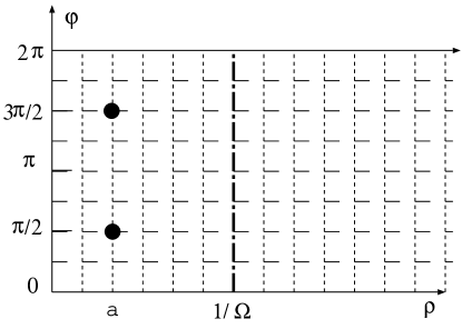
Figure 1: Coordinate regions for the periodic wave equation. The sources are shown as dark circles. The light cylinder is shown as the line with dots and dashes at $\rho=1/\Omega$. The outer boundary, $\rho=\rho_{\rm max}$, is not shown.

The coordinate regions for this equation are shown in Figure 1. Although this figure misrepresents the topology (a disk) of the physical problem, it is the appropriate description of the ($\rho,{\varphi}$) grid on which (5) is to be solved as a finite difference equation. The specific conditions to be used in solving the problem are the following: (i) Due to the symmetry of our source, and to condition (3), the solution is to have the symmetry $\psi(\rho,{\varphi})=-\psi(\rho,{\varphi}+\pi)$. This allows us to restrict the numerical solution to the range $0<{\varphi}<\pi$. (ii) Due to the antisymmetry under ${\varphi}\rightarrow{\varphi}+\pi$, the solution for $\psi$ must vanish at all $\rho=0$ grid points. (iii) Outgoing Sommerfeld boundary conditionsare imposed at some maximum radius ${\rho_{\rm max}}$ by requiring

$$\left.\left(\frac{\partial\psi}{\partial\rho}-\Omega\frac{\partial\psi}{\partial{\varphi}}\right)\right|_{\rho={\rho_{\rm max}}}=0\ .$$ (6)

If (5) and the above conditions (i-iv) are put on a grid of $N_{r}$ radial lines and $N_{{\varphi}}$ lines, containing $N\equiv N_{r}\times N_{{\varphi}}$ grid points with a priori unknown values of $\psi$, a system of $N$ equations for these unknowns is found. The solution of this system is the finite difference solution of our physical problem.

The finite difference procedure just outlined is relatively straightforward, but it has an unusual feature. Note that the nature of the differential equation in (5) changes at the “light cylinder” $\rho=1/\Omega$, shown as a line with dots and dashes in Figure 1. For $\rho<1/\Omega$ the equation is formally elliptic, while for $\rho>1/\Omega$ it is hyperbolic. Typically elliptic partial differential equations are solved as boundary value problems, with auxiliary data given on a closed boundary surrounding the region of the solution, but hyperbolic equations are given Cauchy data on an “initial” hypersurface. The common wisdom is that a hyperbolic problem with data specified on a closed surface can have more than a single solution[12]. Despite this we treat the entire coordinate region ($0\leq{\varphi}<\pi,0\leq r\leq{\rho_{\rm max}}$) as a boundary value problem. We have not attempted to give a rigorous proof that the boundary value approach to (5) and (6) is well posed, but several nonrigorous justifications are worth mentioning: (i) Although nonuniqueness is a possible feature for a hyperbolic equations with boundary values, whether or not a particular problem suffers from this difficulty depends on details of the problem, not only on whether it is hyperbolic. (ii) The physical problem described by the boundary value problem appears to be well posed. (iii) Numerical solutions of the boundary value problem are stable and insensitive to numerical grid size.

Here, as in the next section, it will be useful to separate the complexities of nonlinearity from other issues. To do this we temporarily set $\lambda$ to zero so that (5) becomes a linear equation. The outgoing radiation solution for this problem is easily found, with standard techniques, in the form of a series of Bessel $J_{m}$ and Neumann $N_{m}$ functions. For $\rho\geq a$, this series is

$$\psi_{\rm out}=Q\sum_{m=1,3,5,\ldots{}}(-1)^{(m+1)/2}J_{m}(m\Omega a)\left[N_{m}(m\Omega\rho)\sin{m{\varphi}}-J_{m}(m\Omega\rho)\cos{m{\varphi}}\right]\ .$$ (7)

This solution shows, by example, that there are no hidden difficulties in finding a solution to (5) in the case $\lambda=0$, and hence there is no fundamental problem in using a boundary value approach to solve a problem with outgoing radiation. It also demonstrates explicitly that, at least in the $\lambda=0$ case, the light cylinder $\rho=1/\Omega$ is not a special surface in the problem. Note that (7) gives the solution for waves that are “outgoing at infinity.” Solving the linear problem for waves that are “outgoing” at a finite radius, i.e. , for the boundary conditions in (6), is almost as simple as for true outgoing waves. For $\rho\geq a$, the solution is

$$\psi=\psi_{\rm out}-Q\sum_{m=1,3,5,\ldots{}}(-1)^{(m+1)/2}J_{m}(m\Omega a)J_{m}(m\Omega\rho)\,{\rm Re}\left(\gamma_{m}\rme^{im{\varphi}}\right)\ ,$$ (8)

where

$$\gamma_{m}=\left.-\frac{H^{(1)}_{m}(z)+i\frac{d}{dz}H^{(1)}_{m}(z)}{J_{m}(z)+i\frac{d}{dz}J_{m}(z)}\right|_{z=m\Omega{\rho_{\rm max}}}\ .$$ (9)

Here $H^{(1)}_{m}$ indicates the Hankel function of type 1. From a well known property of Hankel functions[13] the numerator of (9) vanishes as $m\Omega{\rho_{\rm max}}\rightarrow\infty$. This demonstrates that (aside from roundoff and truncation error) a solution on a grid of finite radial extent approaches the true outgoing solution as the radial extent of the grid becomes infinite. We have also checked that there are no difficulties, with truncation or otherwise, in solving (5) with finite difference methods. The solution found in this way was compared with (7). The agreement was excellent, and the expected second order convergence of the finite difference scheme was confirmed.

To investigate a nonlinear model numerically a specific choice must be made for the nonlinear term ${\cal F}$. To suit our purposes this term must satisfy several criteria in addition to the symmetry condition in (3). One criterion is that this nonlinear term be small enough at the outer boundary ${\rho_{\rm max}}$, so that the outgoing condition (6) is a good approximation at a large finite radius. The nature of this requirement can be seen if we choose ${\cal F}$ simply to be $\psi$, so that the nonlinear term in (5) becomes $\lambda\psi$, and (5) is the Helmholtz equation. The “outgoing” solution to this linear problem is that given in (7), except that the arguments of the Bessel and Neumann functions have $\sqrt{m^{2}\Omega^{2}+\lambda}$ in place of $m\Omega$. At large $\rho$ this solution will satisfy the condition (6), for a particular angular Fourier mode, if the $\Omega$ is replaced by $\sqrt{m^{2}\Omega^{2}+\lambda}\,/m$. The standard outgoing condition is then a good approximation only if $|\lambda|\ll\Omega^{2}$. To get a rough idea of the effect of nonlinearities on boundary conditions we can view the nonlinear term $\lambda{\cal F}$ as $\lambda_{\rm eff}\psi$ with $\lambda_{\rm eff}$, the effective $\lambda$, taken to be $\lambda\langle{\cal F}\rangle/\left<\psi\right>$. Here “$\langle\rangle$” indicates some sort of average (perhaps an r.m.s average over all ${\varphi}$ and one wavelength). A rough criterion for a nonlinear term that is compatible with the boundary condition (6) is that $\lambda_{\rm eff}$, at ${\rho_{\rm max}}$, be much smaller than $\Omega^{2}$. For our toy model to have interesting nonlinear effects, however, there is a somewhat contradictory requirement: the nonlinear term must be significant, even dominant, at small radius. A nonlinear term like ${\cal F}=\psi^{3}$ can be strong at small radii and weak at large radii if the field $\psi$ falls off quickly enough. For our line sources, the radiation fields fall off only as $r^{-1/2}$. This slow fall off causes computational difficulties in the application of boundary conditions. For this reason we include a factor $\exp{(-\left(\alpha\rho/a\right)^{2})}$ in the nonlinear term. To be certain that the nonlinear source is sufficiently well behaved near the point sources at the points $(a,\pi/2)$ and $(a,3\pi/2)$, we choose a source term that does not diverge at those points. The specific choice used in our numerical investigations has been

$${\cal F}=\exp(-(\alpha\rho/a)^{2})\frac{\psi^{3}}{\left(\psi^{2}+1\right)^{3/2}}\ .$$ (10)

The outgoing wave pattern for $\psi$ is illustrated in Figure 2. The field $\psi$ is shown as a function of $\rho\cos\phi$ and $\rho\sin\phi$ for two different times: (a) $\Omega t=0$, and (b) $\Omega t=\pi$. The figure illustrates how the rotation of the “rigid” pattern sends waves outward. The results were obtained from numerical runs with $961\times 41$ gridpoints in $\rho\in[0,40]$ and ${\varphi}\in[0,\pi]$. The parameter values are $Q=1$, $\Omega=0.5$, $a=0.5$, $\lambda=1500$, $\alpha=1$. At $\Omega t=0$, the positively charged particle is at $\phi=\pi/2$ and at $\Omega t=\pi$ it is at $\phi=3\pi/2$.

Figure 2: The field $\psi$ as a function of $\rho\cos\phi$ and $\rho\sin\phi$ for the two different times $\Omega t=0$ (a) and $\Omega t=\pi$ (b). This is a numerical solution to the nonlinear wave equation (with nonlinearity parameter $\lambda=1500$ and localization parameter $\alpha=1$) in the presence of outgoing-radiation boundary conditions. The sources are located at a radius of $\rho=0.5$. Note that there are no discernable irregularities at the light cylinder $\rho=2$.

Figure 3 shows the importance of nonlinear effects for the outgoing fields of Figure 2. The field $\psi$ is shown as a function of $\rho$ at ${\varphi}=\pi/2$, for $Q=1$, $\Omega=0.5$, and $a=0.5$. The solid curve shows the solution of the linear problem for $\lambda$ set to zero; the dashed curve shows the nonlinear fields for $\lambda=1500$, $\alpha=1$. Details of the fields near the source particles are shown in the insert. Though the nonlinear terms are negligible in the wave zone, the amplitude of the waves is more than doubled by the increase in the effective source strength produced by the nonlinearity in the central region.

Figure 3: The linear (solid curve) outgoing solution for $\lambda=0$ and the nonlinear (dashed curve) outgoing solution for $\lambda=1500$, $\alpha=1$. Both curves are for $Q=1$, $\Omega=0.5$, and $a=0.5$. The fields are shown at ${\varphi}=\pi/2$. The sharp peaks correspond to the location of the particle, at $\rho=0.5$. Note that there are no discernable irregularities at the light cylinder $\rho=2$.

3 Radiation-balanced boundary conditions

The universality of gravitational coupling in GR means that periodic orbits and outgoing radiation are not compatible. In this section we investigate a choice of solution for our toy model that does seem applicable to periodic orbits in GR. We introduce boundary conditions that do not carry net energy away from the inner region of the orbiting objects, boundary conditions containing equal measures of ingoing and outgoing radiation. There is a temptation to relate this idea to that of “standing waves,” and to impose Dirichlet boundary conditions that $\psi$ vanishes at some “wall” located at $\rho={\rho_{\rm wall}}$. As in the previous section, it is useful to separate issues of nonlinearity from other issues, and to look at the $\lambda=0$ case first. For this linear problem the solution, for $\rho>a$, with $\psi$ vanishing at $\rho={\rho_{\rm wall}}$ is

$$\psi=Q\sum_{m=1,3,5,\ldots{}}(-1)^{(m+1)/2}J_{m}(m\Omega a)\left[N_{m}(m\Omega\rho)+\beta_{m}J_{m}(m\Omega\rho)\right]\sin{m{\varphi}}\ ,$$ (11)

where

$$\beta_{m}=-\frac{N_{m}(m\Omega{\rho_{\rm wall}})}{J_{m}(m\Omega{\rho_{\rm wall}})}\ .$$ (12)

The expressions in (11) and (12) do not describe a well behaved solution. In general, the denominator for $\beta_{m}$ will come arbitrarily close to zero, as larger and larger values of $m$ are included in the sum. We have confirmed that the finite difference solution to (11) and (12) is not stable for small changes in the location of ${\rho_{\rm wall}}$, or for a change in the number of grid points. [Note that increasing the number of angular grid divisions is roughly equivalent to increasing the maximum value of $m$ included in the sum in (11).]

In considering fields $\psi$ that are acceptable mixtures of ingoing and outgoing waves, it is again helpful to look at the linear ($\lambda=0$) problem. In this case, a more-or-less obvious acceptable choice of $\psi$ can be constructed simply by averaging the solutions to (5) with ingoing waves at infinity and with outgoing waves at infinity. The result, for $\rho>a$, is

$$\psi=Q\sum_{m=1,3,5,\ldots{}}(-1)^{(m+1)/2}J_{m}(m\Omega a)N_{m}(m\Omega\rho)\sin{m{\varphi}}\ .$$ (13)

Although this is not the most general solution of the linear problem with equal amounts of in and outgoing waves, it is the most natural solution, as discussed in A.

The field in (13) is a solution to (5) in the $\lambda=0$ case, but not for any simply stated boundary conditions. In particular, it does not correspond to the vanishing of $\psi$ at some specific finite radius. Nor is it the limit in which the “wall” of (11), (12) is at $\infty$; no such limit exists. Rather, it is a superposition of two solutions each of which has a simply stated boundary condition (ingoing or outgoing), and superposition is not valid for solutions of nonlinear equations. We therefore reformulate our toy model so that fields can be found that are the nonlinear equivalent of (13). In place of a partial differential equation, we introduce an integral equation. The first step in doing this is to rewrite (5) as

$${\cal L}\psi=\sigma_{\rm eff}(\rho,{\varphi},\psi)\ ,$$ (14)

where

$${\cal L}\equiv-\frac{1}{\rho}\frac{\partial}{\partial\rho}\rho\frac{\partial}{\partial\rho}-\left(\frac{1}{\rho^{2}}-\Omega^{2}\right)\frac{\partial^{2}}{\partial{\varphi}^{2}}$$ (15)

and

$$\sigma_{\rm eff}(\rho,{\varphi},\psi)\equiv\sigma(\rho,{\varphi})+\lambda{\cal F}(\psi,\rho)\ .$$ (16)

We take the solution of (14-16) to be the time symmetric Green function (TSGF) solution given by

$$\psi_{\rm TSGF}(\rho,{\varphi})=\int\int G_{\rm TS}(\rho,{\varphi};\rho^{\prime},{\varphi}^{\prime})\sigma_{\rm eff}(\rho^{\prime},{\varphi}^{\prime}\psi(\rho^{\prime},{\varphi}^{\prime}))\rho^{\prime}\rmd\rho^{\prime}\rmd{\varphi}^{\prime}\ ,$$ (17)

where the Green function $G_{\rm TS}(\rho,{\varphi};\rho^{\prime},{\varphi}^{\prime})$ is the time symmetric inverse to the linear operator ${\cal L}$ corresponding to equal mixtures of ingoing and outgoing waves. In principle, this Green function can be written explicitly as

$$G(\rho,{\varphi};\rho^{\prime},{\varphi}^{\prime})_{\rm TS}=\cases{-\frac{1}{2\pi}\ln({\rho}/{\rho^{\prime}})-\frac{1}{2}\sum_{m=1}^{\infty}J_{m}(m\Omega\rho^{\prime})N_{m}(m\Omega\rho)\cos m({\varphi}-{\varphi}^{\prime})&$\rho>\rho^{\prime}$\\ -\frac{1}{2}\sum_{m=1}^{\infty}N_{m}(m\Omega\rho^{\prime})J_{m}(m\Omega\rho)\cos m({\varphi}-{\varphi}^{\prime})&$\rho<\rho^{\prime}$}$$

(18)

In practice, this series form of the time symmetric Green function is not directly applicable to our numerical method, and it is more useful to write the same radiation balanced solution with the following symbolic notation. We denote the solution to the nonlinear problem with outgoing boundary conditions as

$$\psi_{\rm out}={\cal L}^{-1}_{\rm out}\sigma_{\rm eff}\ ,$$ (19)

where ${\cal L}^{-1}_{\rm out}$ is the inverse to ${\cal L}$ for outgoing boundary conditions, i.e. , the retarded-time Green function. The ingoing solution $\psi_{\rm in}$ is written in a parallel manner using the advanced-time Green function ${\cal L}^{-1}_{\rm in}$. The linear superposition of the ingoing and outgoing (LSIO) solutions is not itself a solution since the problem is nonlinear.

To arrive at a field $\psi_{\rm TSGF}$ that is a solution, and that corresponds to the solution in (17), we superpose the operators ${\cal L}^{-1}_{\rm in}$ and ${\cal L}^{-1}_{\rm out}$ and take our radiation balanced solution to be

$$\psi_{\rm TSGF}=\frac{1}{2}\left({\cal L}^{-1}_{\rm in}+{\cal L}^{-1}_{\rm out}\right)\sigma_{\rm eff}\equiv{\cal L}^{-1}_{\rm TSGF}\sigma_{\rm eff}.$$ (20)

This integral equation is to be solved by iteration. From $\psi_{{\rm TSGF},n}$, the $n^{\rm th}$ iteration for $\psi_{{\rm TSGF}}$, we construct $\sigma_{{\rm eff},n}$, and then find the $(n+1)^{\rm th}$ iteration of the solution from

$$\psi_{{\rm TSGF},n+1}={\cal L}^{-1}_{\rm TSGF}\sigma_{{\rm eff},n}\ .$$ (21)

This method is well suited to implementation as a finite difference solution to a boundary value problem on a grid of $N$ points, like that in Figure 1. In this implementation, $\psi_{\rm TSGF}$ and $\sigma_{\rm eff}$ are one dimensional vectors of length $N$, and ${\cal L}$, along with the chosen boundary conditions, forms an $N\times N$ matrix. Since the form of this matrix depends on boundary conditions, the numerical inverse ${\cal L}^{-1}$ is also specific to the boundary conditions. The numerical radiation balanced operator ${\cal L}_{\rm TSGF}^{-1}$ is simply the average of the matrix inverses of ${\cal L}^{-1}$ for the ingoing and outgoing problems. Results of this numerical solution are shown in Figure 4. This figure, when compared with Figure 2 nicely illustrates the symmetry of the radiation field with respect to reversal of ${\varphi}$. It is not so effective in illustrating the fact that there is no radius at which $\psi$ vanishes at all values of ${\varphi}$. This is due to the strong dominance of the $m=1$ multipole of the field. For larger values of the source velocity $v=a\Omega$ the $m=3,5,\ldots{}$ multipoles make stronger contributions, but for those values of $v$ for which we could get accurate solutions (up to $v$ around 0.8) the $m=1$ multipole continued to dominate the appearance of the fields in a plot like that in Figure 4.

Figure 4: The field $\psi$ as a function of $\rho\cos\phi$ and $\rho\sin\phi$ (at time $t=0$). This is the numerical solution to the nonlinear wave equation (with nonlinearity parameter $\lambda=1500$ and localization parameter $\alpha=1$) according to the TSGF method of imposing a radiation-balanced boundary condition. The sources are located at a radius of $\rho=0.5$. Note that there are no discernible irregularities at the light cylinder $\rho=2$.

We now argue that within the scope of our approximation, the TSGF solution in the wave zone is close to a linear superposition of the ingoing and outgoing (LSIO) solutions for the same orbiting sources. It is important to recall that due to the nonlinearity, the LSIO is not a solution of (5), but it does have the convenient property that if the nonlinearities are weak in the wave zone, the outgoing and ingoing solutions can easily be extracted from the LSIO. We are claiming then that an approximate outgoing solution to the problem, in the wave zone, can be found from the TSGF solution. We emphasize that we are not claiming that nonlinear effects are weak. We will show that this approximation method is successful for problems with very strong nonlinear effects. The reason for this success can be seen most easily if (20) is rewritten as

$$\psi_{\rm TSGF}=\frac{1}{2}{\cal L}_{\rm in}^{-1}\sigma_{\rm eff}(\psi_{\rm TSGF})+\frac{1}{2}{\cal L}^{-1}_{\rm out}\sigma_{\rm eff}(\psi_{\rm TSGF})$$ (22)

and compared with the LSIO (not a solution of the nonlinear problem),

$$\psi_{\rm LSIO}=\frac{1}{2}{\cal L}_{\rm in}^{-1}\sigma_{\rm eff}(\psi_{\rm in})+\frac{1}{2}{\cal L}^{-1}_{\rm out}\sigma_{\rm eff}(\psi_{\rm out})\ .$$ (23)

The TSGF solution and the LSIO superposition differ due to the nonlinear terms contained within the effective source. Those nonlinear terms will be significant only in the small radius inner regions of the physical space, where the fields are strong. But in the inner, strong field, regions the solution should not be highly sensitive to whether ingoing or outgoing boundary conditions are imposed. Indeed, this last statement is a way of viewing the underlying idea in our approach. If the fields near the orbiting objects are not significantly influenced by the distant boundary conditions, then radiation reaction cannot be important. We are now assuming the converse: with parameters for which radiation reaction is not important, the fields near the sources will not be sensitive to the boundary conditions.

If the nonlinear contributions to $\sigma_{\rm eff}$ are nonnegligible only in the strong field region near the orbiting objects, and if the fields there are insensitive to boundary conditions, then we can conclude that $\sigma_{\rm eff}(\psi_{\rm in})$ and $\sigma_{\rm eff}(\psi_{\rm out})$ differ negligibly. It is then plausible that they are also negligibly different from $\sigma_{\rm eff}(\psi_{\rm TSGF})$, and hence that the LSIO is approximately the same as the TSGF solution. This conclusion, furthermore, should be valid to the same degree that it is valid to ignore radiation reaction (more specifically to ignore the sensitivity of the fields near the source to the boundary conditions on the waves).

For the nonlinearity given by (10), with $\lambda=1500$, $\alpha=1$, it turns out that the approximation of TSGF by LSIO is too good for an effective illustration. In this case a plot shows no discernible difference between the TSGF and LSIO, even though the nonlinearity plays a strong role, as shown in Figure 3. A discernible difference can be seen if the $\alpha$ parameter is reduced. The effect is to spread the region of strong nonlinearity to larger radius where the fields are somewhat sensitive to the boundary conditions. The comparison of the TSGF and the LSIO fields, for $\alpha=0.1$ is shown in Figure 5. The field $\psi$ is shown as a function of $\rho$ both for ${\varphi}=\pi/2$, the angular position of a source particle, and at ${\varphi}=\pi/4$. No difference between the TSGF and the LSIO fields can be seen at small radii. In the radiation zone a small phase shift can be seen between the LSIO and the TSGF and the LSIO waves are seen to have a slightly smaller amplitude.

In our approximation approach, the idea is to find the solution of the outgoing wave amplitude from the TSGF solution, by considering the TSGF solution in the wave zone to be (approximately) an equal mixture of ingoing and outgoing radiation. The specific application of this idea requires fitting the TSGF radiation field to a sum of multipoles of the form

$$\psi_{\rm TSGF}\approx\sum_{m=1,3,5\ldots{}}C_{m}N_{m}(m\Omega\rho)\sin{m{\varphi}},$$ (24)

and from the amplitudes $C_{m}$ inferred from the fit, writing the outgoing solution as

$$\psi_{\rm out}\approx\sum_{m=1,3,5\ldots{}}C_{m}\left[N_{m}(m\Omega\rho)\sin{m{\varphi}}-J_{m}(m\Omega\rho)\cos{m{\varphi}}\right]\ .$$ (25)

Using our toy nonlinear model, we can solve for both the TSGF and the outgoing solution, to check the accuracy of this method. For the model with parameters $Q=1$, $a=0.5$, $\Omega=0.5$, $\lambda=150$, $\alpha=0.1$, fitting the TSGF from $\rho=20$ to $\rho=40$, gives a wave amplitude for outgoing radiation that is larger than the true amplitude by 24%. For $\alpha=1$ the discrepancy is only 0.04%.

Figure 5: The difference between TSGF and LSIO. The figures show the source region and the wave zone for $a=0.5$, $\Omega=0.5$, $\alpha=0.1$ and $\lambda=150$. The plot on the right is for ${\varphi}=\pi/4$ and that on the left is for ${\varphi}=\pi/2$, the ${\varphi}$ location of one of the particles.

4 Conclusion and discussion

For our nonlinear toy scalar field model, we have demonstrated that a radiation balanced field, the time symmetric Green function (TSGF) solution, can be found by solving a numerical problem similar to a boundary value problem. Although the character of the differential operator is elliptical inside the light cylinder and hyperbolic outside, no special treatment of this surface was necessary, and the solution was found with boundary value methods usually associated with elliptical equations, despite the outer boundary being in the “hyperbolic” region. We have also shown that to the extent that radiation reaction forces can be ignored, the TSGF solution is a good approximation to the solution with outgoing boundary conditions.

We must now ask how related methods might be brought to bear on the problem of orbiting objects in GR. An important feature of the nonlinear scalar toy model is that the nonlinearities in the theory do not occur in the wave operator. This allowed us directly to recast the problem as an integral equation by using the time-symmetric Green function for the wave operator. It is not at all clear how the GR equations can be cast in a form with a linear wave operator, or whether it is in principle impossible. But it is not necessary that we follow these same steps in dealing with the GR equations. What is required, most generally, is any method for specifying a time symmetric solution.

For such a method in GR it is expected that some features of the basic physics will be the same as in the scalar model. In particular, for motions $\tau_{orb}/\tau_{rad}\ll 1$ the nonlinear terms in the effective source should be insensitive to boundary conditions. It can then be supposed that the radiation balanced solution is a good approximation to the linear superposition of ingoing and outgoing solutions (LSIO) and that from the LSIO we can infer the outgoing solution. There is, however, an important difference between this claim as it applies to GR, and the (demonstrably true) claim for the scalar field model. In the scalar field model we were comparing LSIO fields for periodic motion with the TSGF solution for periodic motion. In GR, there can be no LSIO solution for periodic motion, since ingoing, or outgoing, energy flux would be incompatible with periodic motion. For GR, the analogy needs to be made directly to the solution with outgoing waves and a slow rate of orbital decay due to radiation reaction. By constructing a spacetime with only outgoing radiation from the TSGF solution, we arrive at an approximation in which the radiation fields are periodic, with a period that is constant, not slowly drifting in time. In the notation introduced in Section 1, the quasi-stationary method in GR requires that the type-III problem be solved and used to produce an approximation to the type-I physics.

An additional complication is that the spacetime of the TSGF fields cannot be asymptotically flat in GR, since there is an infinite amount of energy contained in the radiation fields[11]. This apparent pathology can be viewed as irrelevant if we think of our TSGF, or outgoing, solutions as being an approximation only in a finite central region of the space. It is worth noting that this viewpoint is consistent with the nature of the numerical solution that is based on boundary conditions applied at finite radius. The important question that remains is whether the inner region, the region in which the problem is solved, is large enough to include a zone in which waves are weak and in which the ingoing and outgoing waves of the approximate LSIO can be disentangled. To investigate this, we note that the gravitational wave luminosity of the binary is of order $L_{\rm GW}\sim(GM/ac^{2})^{5}(c^{5}/G)$, where we are using the same notation as for (1). The gravitational wave energy $E_{\rm GW}$ contained within a sphere of radius ${\rho_{\rm max}}$ is of order $L_{\rm GW}{\rho_{\rm max}}/c$, and hence the ratio of $E_{\rm GW}$ to the orbital energy $GM^{2}/a$ of the binary, is of order

$$\frac{E_{\rm GW}}{GM^{2}/a}\sim\left(\frac{GM}{ac^{2}}\right)^{3}\frac{{\rho_{\rm max}}}{a}\ .$$ (26)

The nature of our approximation requires that $GM/(ac^{2})$ be small, so we conclude that the gravitational wave energy contained within ${\rho_{\rm max}}$ will be much less than the orbital energy, even for values of ${\rho_{\rm max}}$ large compared to $a$.

This last conclusion is important if we are to hope to use versions of our method to make inferences about the ISCO. By investigating the dependence of the binary energy on radius, we can study whether there is an instability like that for particles. The “energy” of the orbit must be computed as a surface integral at a large radius. If this integral were significantly influenced by the energy contained in the waves, conclusions about orbital stability would be suspect.

Whether or not the methods of this paper can be applied to the ISCO question, the use of these methods in GR would provide an important addition to the tools needed to understand black hole inspiral. A direct and obvious use of the method would be to provide Cauchy data for numerical relativity.

Appendix A General Radiation-Balanced Solution

We present here some of the details of the general solution for the linear scalar field theory with equal flux of ingoing and outgoing radiation. The Green function $G(\rho,{\varphi};\rho^{\prime},{\varphi}^{\prime})$ for the linear problem satisfies

$$\left[\frac{1}{\rho}\frac{\partial}{\partial\rho}\rho\frac{\partial}{\partial\rho}+\left(\frac{1}{\rho^{2}}-\Omega^{2}\right)\frac{\partial^{2}}{\partial{\varphi}^{2}}\right]G(\rho,{\varphi};\rho^{\prime},{\varphi}^{\prime})=-\rho^{\prime-1}\delta(\rho-\rho^{\prime})\delta({\varphi}-{\varphi}^{\prime}).$$ (27)

When the ${\varphi}$ dependence is represented in a Fourier series, and the Green function is written as $G(\rho,{\varphi};\rho^{\prime},{\varphi}^{\prime})$ =Re$\left[\sum{\cal G}_{m}(\rho;\rho^{\prime},{\varphi}^{\prime})\rme^{im{\varphi}}\right]$ , the equation becomes

$$\left[\frac{1}{\rho}\frac{\partial}{\partial\rho}\rho\frac{\partial}{\partial\rho}+m^{2}\left(\Omega^{2}-\frac{1}{\rho^{2}}\right)\right]{\cal G}_{m}(\rho;\rho^{\prime},{\varphi}^{\prime})=-\frac{1}{2\pi\rho^{\prime}}\delta(\rho-\rho^{\prime})\rme^{-im{\varphi}^{\prime}}$$ (28)

Reality of the Green function $G(\rho,{\varphi};\rho^{\prime},{\varphi}^{\prime})$ means that ${\cal G}_{-m}(\rho;\rho^{\prime},{\varphi}^{\prime})={\cal G}_{m}(\rho;\rho^{\prime},{\varphi}^{\prime})^{*}$, and the $m=0$ mode is irrelevant for the sources we consider, so we only need the general solution to (28) for $m>0$, which is

$${\cal G}_{m}(\rho;\rho^{\prime},{\varphi}^{\prime})=\cases{-\frac{1}{4}J_{m}(m\Omega\rho^{\prime})N_{m}(m\Omega\rho)\rme^{-im{\varphi}^{\prime}}+\Gamma_{m}(\rho^{\prime},{\varphi}^{\prime})J_{m}(m\Omega\rho)&$\rho>\rho^{\prime}$\\ -\frac{1}{4}N_{m}(m\Omega\rho^{\prime})J_{m}(m\Omega\rho)\rme^{-im{\varphi}^{\prime}}+\Gamma_{m}(\rho^{\prime},{\varphi}^{\prime})J_{m}(m\Omega\rho)&$\rho<\rho^{\prime}$}$$ (29)

For $\rho>\rho^{\prime}$, ${\cal G}_{m}$ can be written in terms of Hankel functions as

$${\cal G}_{m}=A_{m}H^{(1)}_{m}(m\Omega\rho)+B_{m}H^{(2)}_{m}(m\Omega\rho)\ ,$$ (30)

where

$$A_{m} = \frac{1}{2}\Gamma_{m}(\rho^{\prime},{\varphi}^{\prime})-\frac{1}{8i}J_{m}(m\Omega\rho)\rme^{-im{\varphi}^{\prime}}$$

$$B_{m} = \frac{1}{2}\Gamma_{m}(\rho^{\prime},{\varphi}^{\prime})+\frac{1}{8i}J_{m}(m\Omega\rho)\rme^{-im{\varphi}^{\prime}}\ .$$ (31)

The condition for equal flux of ingoing and outgoing radiation is $|A_{m}|=|B_{m}|$, for all $m$. This, and the expressions in (31), require that $\Gamma_{m}(\rho^{\prime},{\varphi}^{\prime})$ be a real multiple of $J_{m}(m\Omega\rho)\rme^{-im{\varphi}^{\prime}}$. The proportionality constant may be different for each $m$, so the general radiation balanced solution is

$${\cal G}_{m}(\rho;\rho^{\prime},{\varphi}^{\prime})=\cases{-\frac{1}{4}J_{m}(m\Omega\rho^{\prime})N_{m}(m\Omega\rho)\rme^{-im{\varphi}^{\prime}}+g_{m}J_{m}(m\Omega\rho^{\prime})J_{m}(m\Omega\rho)\rme^{-im{\varphi}^{\prime}}&$\rho>\rho^{\prime}$\\ -\frac{1}{4}N_{m}(m\Omega\rho^{\prime})J_{m}(m\Omega\rho)\rme^{-im{\varphi}^{\prime}}+g_{m}J_{m}(m\Omega\rho^{\prime})J_{m}(m\Omega\rho)\rme^{-im{\varphi}^{\prime}}&$\rho<\rho^{\prime}$}$$

Any choice of the set of real constants $g_{m}$ gives a radiation balanced solution. The choice made for the TSGF solution, $g_{m}=0$, for all $m$, is convenient for a numerical implementation that does not explicitly use Fourier decomposition. The choice $g_{m}=0$ also seems to be the most natural one if one views the $\Gamma_{m}$ terms in (28) as free waves, disconnected from the source.

Appendix B Three-plus-One Dimensional Theory

Here we present the solution of a linear toy model for point-like sources. We use standard spherical coordinates ($r,\theta,\phi$) and suppose that two particles of opposite scalar charge $\pm Q$ orbit at frequency $\Omega$ in the equatorial plane ($\theta=\pi/2$), at radius $a$, with angular separation $\Delta\phi=\pi$. In the linear differential equation of this toy model

$$\nabla^{2}\psi-\partial_{t}^{2}\psi=-a^{-2}Q\delta(r-a)\delta(\cos\theta)\left[\delta(\phi-\Omega t-\pi/2)-\delta(\phi-\Omega t-3\pi/2)\right]\ ,$$ (33)

we make the ansatz that the solution is not of the general type $\psi(r,\theta,\phi,t)$, but rather of the type $\psi(r,\theta,\varphi)$ where $\varphi\equiv\phi-\Omega t$. The differential equation then reduces to the point-like linear analog of (5):

$$\frac{1}{r^{2}}\frac{\partial}{\partial r}\left(r^{2}\frac{\partial\psi}{\partial r}\right)+\frac{1}{r^{2}\sin\theta}\frac{\partial}{\partial\theta}\left(\sin\theta\frac{\partial\psi}{\partial\theta}\right)+\left[\frac{1}{r^{2}\sin^{2}\theta}-\Omega^{2}\right]\frac{\partial^{2}\psi}{\partial{\varphi}^{2}}$$

$$=a^{-2}Q\delta(\rho-a)\delta(\cos\theta)\left[\delta({\varphi}-\pi/2)-\delta({\varphi}-3\pi/2)\right]\ .$$ (34)

If $\psi(r,\theta,\varphi)$ is decomposed as a sum of spherical harmonics $Y_{\ell m}(\theta,\varphi)$ it is straightforward to find the solution that is well behaved at $r=0$ and that corresponds to outgoing waves at infinity. This solution, the point-like equivalent of (7), is

$$\psi(r,\theta,\varphi)=Q\Omega\sum_{\ell m}\kappa_{\ell m}Y_{\ell m}(\theta,\varphi)\times\cases{j_{\ell}(m\Omega a)h^{(1)}_{\ell}(m\Omega r)&$r>a$\\ j_{\ell}(m\Omega r)h^{(1)}_{\ell}(m\Omega a)&$r<a$}$$ (35)

Here $j_{\ell}$ and $h^{(1)}_{\ell}$ indicate spherical Bessel and Hankel functions. The sum in (35) is over odd $\ell$ and odd $m$, and the coefficients $\kappa_{\ell m}$ are given by

$$\kappa_{\ell m}=im\left[Y_{\ell m}^{*}(\pi/2,\pi/2)-Y_{\ell m}^{*}(\pi/2,3\pi/2)\right]=(-1)^{(m-1)/2}2mY_{\ell m}(\pi/2,0)\ .$$ (36)

The point-like equivalent of (13), the radiation balanced TSGF solution of the problem, is

$$\psi(r,\theta,\varphi)=iQ\Omega\sum_{\ell m}\kappa_{\ell m}Y_{\ell m}(\theta,\varphi)\times\cases{j_{\ell}(m\Omega a)n_{\ell}(m\Omega r)&$r>a$\\ j_{\ell}(m\Omega r)n_{\ell}(m\Omega a)&$r<a$}$$ (37)

where $n_{\ell}$ is the spherical Neumann function. These solutions serve as explicit illustrations that for point-like sources in 3+1 dimensions the field embodies the same symmetry as the sources. That is, the field rotates “rigidly.” The dependence on time and on azimuthal angle appears only in the combination $\phi-\Omega t$.

Appendix C Net Force on the Orbiting Particles

In this appendix, we show that for a general radiation-balanced solution to the problem of orbiting particles, the proscribed circular orbits of the particles are consistent with the scalar field equations of motion without the need for external forces. (This is not true in the case of purely outgoing radiation.) We limit attention to the linear theory, so that we can easily separate out the forces due to each particle on the other, without worrying about any self-force.

The covariant force law for a scalar-charged particle with charge $Q$, mass $m$, and energy-momentum vector $p$ moving in a scalar field $\psi$ gives a force of

$$m^{-1}p^{\nu}\nabla_{\nu}p^{\mu}=\frac{\rmd p^{\mu}}{\rmd\tau}+m^{-1}\Gamma^{\mu}_{\nu\lambda}p^{\nu}p^{\lambda}=-Q\nabla^{\mu}\psi\ .$$ (38)

If we work in co-rotating coordinates, in which the particle is momentarily at rest, the metric is

$$\rmd s^{2}=-(1-\Omega^{2}\rho^{2})\rmd t^{2}+\rmd\rho^{2}+\rho^{2}\rmd\varphi^{2}+2\Omega\rho^{2}\rmd\varphi\rmd t$$ (39)

and the only non-zero component of the energy-momentum vector is

$$p^{t}=(1-\Omega^{2}a^{2})^{-1/2}m=:\gamma m\ ,$$ (40)

so that the only relevant Christoffel symbol is $\Gamma^{\rho}_{tt}$. (In the corresponding calculation in the 3+1 dimensional theory, only $\Gamma^{r}_{tt}$ is relevant.)

The equations of motion for $p^{\rho}$ and $p^{\varphi}$ in the 2+1 dimensional theory thus become

$$\frac{\rmd p^{\rho}}{\rmd\tau}=-Q\psi_{,\rho}+\gamma^{2}m\rho\Omega^{2}$$ (41)

$$\frac{\rmd p^{\varphi}}{\rmd\tau}=-Qg^{\varphi\varphi}\psi_{,\varphi}\ ,$$ (42)

where we have used the form of the inverse metric $g_{\mu\nu}$ in co-rotating coordinates and the fact that $(\partial\psi/\partial t)_{\varphi}=0$. The second term in (41) represents the fictitious centrifugal force that the particle feels in the co-rotating reference frame. The radial momentum $p^{\rho}$ can remain zero if the repulsive effect of this term cancels the attraction due to the field, described in the first term. This implies a relationship among the orbital radius $a$, angular frequency $\Omega$, and charge-to-mass ratio $Q/m$. (The corresponding relationship is given for orbiting charged particles in the presence of a half-advanced, half-retarded electromagnetic potential in [14].)

The angular force in (42), which represents radiation reaction force, will vanish if (and only if) the scalar field due to one particle has vanishing $\varphi$ derivative at the location of the other particle. For concreteness, we consider the force on the positively-charged particle at $\rho=a$, $\varphi=\pi/2$ due to the negatively-charged particle at $\rho=a$, $\varphi=3\pi/2$. The field due to the latter particle is

$$\psi(\rho,\varphi)=-QG(\rho,\varphi;a,3\pi/2)\ ,$$ (43)

where $G(\rho,\varphi;\rho^{\prime},\varphi^{\prime})$ is the Green function used to construct the solution. Using the Fourier expansion of the Green function given in A, we find that

$$\psi_{,\varphi}(a,\pi/2)=-{\rm Re}\left[\sum_{m}im\left(\frac{1}{4}J_{m}(m\Omega a)N_{m}(m\Omega a)(-1)^{m}+\Gamma_{m}(a,3\pi/2)\rme^{im\pi/2}\right)\right]\ .$$ (44)

This vanishes if the quantity in large parentheses on the right-hand side is real; for a general radiation-balanced solution this is the case, since $\Gamma_{m}(a,3\pi/2)=g_{m}J_{m}(m\Omega a)\exp(-im3\pi/2)$ with $g_{m}$ real. Thus the radiation-balanced solutions have zero radiation reaction force.

However, in the case of purely outgoing radiation, $\Gamma_{m}(\rho^{\prime},\varphi^{\prime})=J_{m}\rme^{-im\varphi^{\prime}}/4i$, and we can explicitly find the radiation reaction force as

$$\psi_{,\varphi}(a,\pi/2)=-\sum_{m}(-1)^{m}\frac{m}{4}[J_{m}(m\Omega a)]^{2}\neq 0\ .$$ (45)

A similar demonstration can be made in the 3+1-dimensional case using the outgoing-radiation and radiation-balanced fields (35) and (37), using the symmetries of the spherical Bessel functions under changes of sign in their arguments to illustrate that terms in the radiation-reaction force due to terms with opposite signs of $m$ cancel each other out in the radiation-balanced mode expansion but not in the outgoing-radiation one.

References

References

- [1] Flanagan É É and Hughes S A 1998 Phys. Rev.D57 4535(Flanagan É É and Hughes S A 1997 Preprint gr-qc/9701039)
- [2] E. Poisson 1998 Preprint gr-qc/9801038
- [3] Numerical relativity applied to black hole inspiral has been the subject of a Grand Challenge computational project. For information visit: http://www.npac.syr.edu/projects/bh/.
- [4] Pullin J 1998 Preprint gr-qc/9803005
- [5] Blackburn J K and Detweiler S 1992 Phys. Rev.D46 2318 Detweiler S 1994 Phys. Rev.D50 4929
- [6] Anninos O, Hobill D, Seidel E, Smarr L, and Suen W-M 1993 Phys. Rev. Lett.71 2851
- [7] Cook G B, Shapiro S L and Teukolsky S A 1996 Phys. Rev.D53 5533Cook G B, Shapiro S L and Teukolsky S A 1995 Preprint gr-qc/9512009
- [8] Wilson J R and Mathews G J 1995 Phys. Rev. Lett.75 4161 Wilson J R, Mathews G J and Marronetti P 1996 Phys. Rev.D54 1317 Wilson J R, Mathews G J and Marronetti P 1996 Preprint gr-qc/9601017
- [9] Whelan J T “Quasistationary binary inspiral III: Gravitational waves on a cylindrically symmetric background” (unpublished)
- [10] Whelan J T and Romano J D 1999 Phys. Rev.D60 084009 Whelan J T and Romano J D 1998 Preprint gr-qc/9812041
- [11] Gibbons G W and Stewart J M 1983 Classical General Relativity ed Bonnor W B et al (Cambridge: Cambridge University Press)
- [12] Mathews J and Walker R L 1970 Mathematical Methods of Physics sec 8.2 (Reading: W. A. Benjamin)
- [13] Olver F W J 1964 Handbook of Mathematical Functions ed Abramowitz M and Stegun I A (Washington: National Bureau of Standards)
- [14] Schild A 1963 Phys. Rev.131, 2762