Stability and Rotational Mixing of Modes in Newtonian and Relativistic Stars

A Dissertation Submitted in
Partial Fulfillment of the
Requirements for the degree of

Doctor of Philosophy

in
Physics

at

The University of Wisconsin-Milwaukee

August, 1999

A Dissertation Submitted in
Partial Fulfillment of the
Requirements for the degree of

Doctor of Philosophy

in
Physics

at

The University of Wisconsin-Milwaukee

August, 1999

          John L. Friedman Date

    Graduate School Approval Date

© Copyright 1999
by
Keith H. Lockitch

Chapter 1 Introduction

1.1 Background and Motivation

This dissertation examines a new class of oscillation modes of rotating stars. The work has been motivated by the recently discovered r-mode instability (see below), and answers a number of previously unresolved questions concerning the nature of the r-mode spectrum in newtonian and relativistic stellar models.

The structure and stability of rotating relativistic stars has recently been reviewed in detail (Stergioulas [75], Friedman [22, 23], Friedman and Ipser [24]), and a general discussion of the small oscillations of relativistic stars may be found in a recent review article by Kokkotas [40] (see also Kokkotas and Schmidt [41]). In this work, we will focus our attention on non-radial oscillations, which were first studied in relativistic stars by Thorne and collaborators (Thorne and Campolattaro [79], Price and Thorne [63], Thorne [76, 77], Campolattaro and Thorne [11], Ipser and Thorne [35]).

The spherical symmetry of a non-rotating star implies that its perturbations can be divided into two classes, polar or axial, according to their behaviour under parity. Where polar tensor fields on a 2-sphere can be constructed from the scalars $Y_{l}^{m}$ and their gradients $\nabla Y_{l}^{m}$ (and the metric on a 2-sphere), axial fields involve the pseudo-vector $\hat{r}\times\nabla Y_{l}^{m}$, and their behavior under parity is opposite to that of $Y_{l}^{m}$. That is, axial perturbations of odd $l$ are invariant under parity, and axial perturbations with even $l$ change sign.

It is useful to further divide stellar perturbations into subclasses according to the physics dominating their behaviour. This classification was first developed by Cowling [16] for the polar perturbations of newtonian polytropic models. The f- and p-modes are polar-parity modes having pressure as their dominant restoring force. They typically have large pressure and density perturbations and high frequencies (higher than a few kilohertz for neutron stars). The other class of polar-parity modes are the g-modes, which are chiefly restored by gravity. They typically have very small pressure and density perturbations and low frequencies. Indeed, for isentropic stars, which are marginally stable to convection, the g-modes are all zero-frequency and have vanishing perturbed pressure and density (see Sect. 2.1). Similarly, all axial-parity perturbations of newtonian perfect fluid models have zero frequency in a non-rotating star. The perturbed pressure and density as well as the radial component of the fluid velocity are all rotational scalars and must have polar parity. Thus, the axial perturbations of a spherical star are simply stationary horizontal fluid currents (see Sect. 2.1).

The analogues of these modes in relativistic models of neutron stars have been studied by many authors. More recently, an additional class of outgoing modes has been identified that exist only in relativistic stars. Like the modes of black holes, these are essentially associated with the dynamical spacetime geometry and have been termed w-modes, or gravitational wave modes. Their existence was first argued by Kokkotas and Schutz [42]. The polar w-modes were first found by Kojima [37] as rapidly damped modes of weakly relativistic models, while the axial w-modes were first studied by Chandrasekhar and Ferrari [14] as scattering resonances of highly relativistic models. (See the reviews by Kokkotas [40] and Kokkotas and Schmidt [41].)

In general, this classification of modes also describes the oscillations of rotating stars, although the character of the modes may be significantly affected by rotation. Because a rotating star is also invariant under parity, its perturbations can be classified according to their behaviour under parity. If a mode varies continuously along a sequence of equilibrium configurations that starts with a spherical star and continues along a path of increasing rotation, the mode will be called axial if it is axial for the spherical star. Its parity cannot change along the sequence, but $l$ is well-defined only for modes of the spherical configuration.

Rotation imparts a finite frequency to the axial-parity perturbations of newtonian models. Because these modes are restored by the Coriolis force, their frequencies are proportional to the star’s angular velocity, $\Omega$. These rotationally restored axial modes were first studied by Papaloizou and Pringle [60], who called them r-modes because of their similarity to the Rossby waves of terrestrial meteorology. For a normal mode of the form $e^{i(\sigma t+m\varphi)}$, Papaloizou and Pringle found the r-mode frequency to be,

$$\sigma+m\Omega=\frac{2m\Omega}{l(l+1)}.$$ (1)

It is only rather recently that the oscillation modes of rotating relativistic stars have begun to be accessible to numerical study (see below). Early work on the perturbations of such stars focused mainly on the criteria for their stability, and led to the surprising discovery that all rotating perfect fluid stars are subject to a non-axisymmetric instability driven by gravitational radiation. The instability was discovered by Chandrasekhar [12] in the $l=m=2$ polar mode of the uniform-density, uniformly rotating Maclaurin spheroids. Although this mode is unstable only for rapidly rotating models, by looking at the canonical energy of arbitrary initial data sets, Friedman and Schutz [28] and Friedman [21] showed the instability to be a generic feature of rotating perfect fluid stars.

In essence, the CFS (Chandrasekhar-Friedman-Schutz) instability operates by converting the rotational energy of the star partly into the oscillation energy of the perturbation and partly into gravitational waves. For a normal mode of the form $e^{i(\sigma t+m\varphi)}$ this nonaxisymmetric instability acts in the following manner.

In a non-rotating star, gravitational radiation removes positive angular momentum from a forward moving mode and negative angular momentum from a backward moving mode, thereby damping all time-dependent, non-axisymmetric modes. In a star rotating sufficiently fast, however, a backward moving mode can be dragged forward as seen by an inertial observer; and it will then radiate positive angular momentum. The mode continues to carry negative angular momentum because the perturbed star has lower total angular momentum than the unperturbed star. As positive angular momentum is removed from a mode with negative angular momentum, the angular momentum of the mode becomes increasingly negative, implying that the amplitude of the mode increases. Thus, the mode is driven by gravitational radiation.

Since the instability acts on modes that are retrograde with respect to the star, but prograde as seen by an inertial observer, a mode will be unstable if and only if its frequency satisfies the condition,

$$\sigma(\sigma+m\Omega)<0.$$ (2)

For the polar f- and p-modes, the frequency is large and approximately real. Condition (2) will be met only if $|m\Omega|$ is of order $|\sigma|$, so that for a given angular velocity the instability will set in first through modes with large $m$.

The CFS instability spins a star down by allowing it to radiate away its angular momentum in gravitational waves. However, to determine whether this mechanism may be responsible for limiting the rotation rates of actual neutron stars, one must also consider the effects of viscous damping on the perturbations. Detweiler and Lindblom [19] suggested that viscosity would stabilize any mode whose growth time was longer than the viscous damping time, and this was confirmed by Lindblom and Hiscock [49]. Recent work has indicated that the gravitational-wave-driven instability can only limit the rotation rate of hot neutron stars, with temperatures above the superfluid transition point, $T\sim 10^{9}\mbox{K}$, but below the temperature at which bulk viscosity apparently damps all modes, $T\sim 10^{10}\mbox{K}$. (Ipser and Lindblom [33]; Lindblom [47] and Lindblom and Mendell [51]) Because of uncertainties in the temperature of the superfluid phase transition and in our understanding of the dominant mechanisms for effective viscosity, even this brief temperature window is not guaranteed.

To calculate the timescales associated with viscous and radiative dissipation it is necessary to compute explicitly the normal modes of oscillation. Until recently, the polar f- and p-modes were expected to dominate the CFS instability through their coupling to mass multipole radiation. As we have already noted, all axial-parity fluid oscillations are time-independent in a spherical model, and therefore do not couple to gravitational radiation at all. (Thorne and Campolattaro [79]) In a rotating star, the rotationally restored r-modes do couple to current multipole radiation. However, their low frequencies and negligible perturbed densities in newtonian stars made it seem implausible that their contribution to gravitational radiation would compare to that of the polar-parity modes.

Indeed, apart from studies of the axial-parity oscillations of models of the neutron star crust (van Horn [80], Schumaker and Thorne [71]), the axial modes were almost universally ignored in the early research on perturbations of relativistic stars. It has only been recently that interest in these modes has been revived, following the work of Chandrasekhar and Ferrari on the resonant scattering of axial wave modes [14] and on the coupling between axial and polar modes induced by stellar rotation [13]. (Further recent studies of axial modes are reviewed by Kokkotas [40] and Kokkotas and Schmidt [41].)

Thus, the first explicit calculations of the dissipative timescales associated with neutron star oscillations focused on the $l=m$ f-modes (Ipser and Lindblom [33], Lindblom [47], Lindblom and Mendell [51]), and until very recently it was only these modes that had been studied in connection with the CFS instability. It has long been hoped that some neutron stars rotate sufficiently fast to be subject to the CFS instability, and that the gravitational radiation produced might be detectable by gravitational wave observatories. However, based on the initial studies of dissipation in f-mode oscillations, the prospects were rather unpromising. Neutron stars formed from stellar collapse would certainly be hot enough to pass through the temperature window at which viscous damping is apparently suppressed, but there was little evidence that neutron stars formed in supernovae (or by the accretion-induced collapse of white dwarves) rotate rapidly enough for the onset of instability. Following an early suggestion of Papaloizou and Pringle [61], Wagoner [81] had proposed another scenario in which an old, accreting neutron star, spun up past the onset of nonaxisymmetric instability would achieve an equilibrium state with angular momentum acquired by accretion balanced by angular momentum radiated in gravitational waves. This scenario, too, appeared to have been ruled out by the strength of damping by mutual friction and viscosity at the temperatures expected for such stars, $T\sim 10^{8}\mbox{K}$.

Very recently, however, a series of surprising results have emerged that dramatically improve these prospects.

The first surprise was the discovery that the r-modes are CFS unstable in perfect fluid models with arbitrarily slow rotation. First indicated in numerical work by Andersson [2], the instability is implied in a nearly newtonian context by the newtonian expression for the r-mode frequency (1), which satisfies the CFS instability criterion, (2), for arbitrarily small $\Omega$,

$$\sigma(\sigma+m\Omega)=-\frac{2(l-1)(l+2)m^{2}\Omega^{2}}{l^{2}(l+1)^{2}}<0.$$ (3)

A computation by Friedman and Morsink [25] of the canonical energy of initial data showed (independent of assumptions on the existence of discrete modes) that the instability is a generic feature of axial-parity fluid perturbations of relativistic stars.

As we have just observed, the generic instability of perfect fluid models will be of no astrophysical importance if, in actual stars, the unstable modes are damped by viscous dissipation. Studies of the viscous and radiative timescales associated with the r-modes (Lindblom et al. [54], Owen et al. [59], Andersson et al. [3], Kokkotas and Stergioulas [43], Lindblom et al. [53]) have revealed a second surprising result: The growth time of r-modes driven by current-multipole gravitational radiation is significantly shorter than had been expected. In fact, it has turned out be so short for some of the r-modes that their instability to gravitational radiation reaction easily dominates viscous damping in hot, newly formed neutron stars. A neutron star that is rapidly rotating at birth now appears likely to spin down by radiating most of its angular momentum in gravitational waves. (See, however, the caveats indicated below.)

Hot on the heels of these theoretical surprises was the discovery by Marshall et.al. [57] of a fast (16ms) pulsar in a supernova remnant (N157B) in the Large Magellanic Cloud. Estimates of the initial period put it in the 6-9ms range, thus providing the long-sought evidence of a class of neutron stars that are formed rotating rapidly. Hence, the newly discovered instability appears to set the upper limit on the spin of the newly discovered class of neutron stars!

The current picture that has emerged of the spin-down of a hot, newly formed neutron star can be readily understood in terms of a model of the r-mode instability due to Owen, Lindblom, Cutler, Schutz, Vecchio and Andersson (hereafter OLCSVA) [59]. Since one particular mode (with spherical harmonic indices $l=m=2$ and frequency $\sigma=-4\Omega/3$) is expected to dominate the r-mode instability, the perturbed star is treated as a simple system with two degrees of freedom: the uniform angular velocity $\Omega$ of the equilibrium star, and the (dimensionless) amplitude $\alpha$ of the $l=m=2$ r-mode. Initially, the neutron star forms with a temperature large enough for bulk viscosity to damp any unstable modes, $T\mathrel{\mathchoice{\vbox{\offinterlineskip\halign{\hfil$\displaystyle#$\hfil\cr>\cr\sim\cr}}}{\vbox{\offinterlineskip\halign{\hfil$\textstyle#$\hfil\cr>\cr\sim\cr}}}{\vbox{\offinterlineskip\halign{\hfil$\scriptstyle#$\hfil\cr>\cr\sim\cr}}}{\vbox{\offinterlineskip\halign{\hfil$\scriptscriptstyle#$\hfil\cr>\cr\sim\cr}}}}10^{10}\mbox{K}$; the star is assumed to be rotating close to its maximum (Kepler) velocity, $\Omega_{K}\sim\sqrt{M/R^{3}}$, the angular velocity at which a particle orbits the star’s equator. The star then cools by neutrino emission at a rate given by a standard power law cooling formula (Shapiro and Teukolsky [72]). Once it reaches the temperature window at which the $l=m=2$ r-mode can go unstable, the system is assumed to evolve in three stages.

First, the amplitude of the r-mode undergoes rapid exponential growth from some arbitrary tiny magnitude. Using conservation of energy and angular momentum, OLCSVA derive the following equations for the evolution of the system in this stage.

$$\frac{d\Omega}{dt}=-\frac{2\Omega}{\tau_{V}}\frac{\alpha^{2}Q}{1+\alpha^{2}Q}$$ (4)

$$\frac{d\alpha}{dt}=\frac{\alpha}{|\tau_{GR}|}-\frac{\alpha}{\tau_{V}}\frac{1-\alpha^{2}Q}{1+\alpha^{2}Q}$$ (5)

Here, $\tau_{GR}$ and $\tau_{V}$ are, respectively, the timescales for the growth of the mode by gravitational radiation reaction and the damping of the mode by viscosity (see Sect. 2.6). (The parameter $Q$ is a constant of order 0.1 related to the initial angular momentum and moment of inertia of the equilibrium star.) Since the initial amplitude $\alpha$ of the mode is so small, the angular momentum changes very little at first (Eq. (4)). That this stage is characterized by the rapid exponential growth of $\alpha$ is the statement that the first term in Eq. (5) (the radiation reaction term) dominates over the second (viscous damping).

Eventually the mode will grow to a size at which linear perturbation theory is insufficient to describe its behaviour. It is expected that a non-linear saturation will occur, halting the growth of the mode at some amplitude of order unity, although the details of these non-linear effects are poorly understood at present. When this saturation occurs, the system enters a second evolutionary stage during which the mode amplitude remains essentially unchanged and the angular momentum of the star is radiated away. During this stage OLCSVA evolve their model system according to the equations

$$\alpha^{2}=\kappa$$ (6)

$$\frac{d\Omega}{dt}=-\frac{2\Omega}{|\tau_{GR}|}\frac{\kappa Q}{1-\kappa Q}$$ (7)

where $\kappa$ is constant of order unity parameterizing the uncertainty in the degree of non-linear saturation. The star spins down by Eq. (7), radiating away most of its angular momentum while continuing to cool gradually.

When its temperature and angular velocity are low enough that viscosity again dominates the gravitational-wave-driven instability, the mode will be damped. During this third stage, OLCSVA return to Eqs. (4)-(5) to continue the evolution of their system. That the mode amplitude decays is the statement that the second term in Eq. (5) (the viscous damping term) dominates the first (radiation reaction), at this temperature and angular velocity.

The net effect of this three-stage evolutionary process is that the newly formed neutron star is left with an angular velocity small compared with $\Omega_{K}$. This final angular velocity appears to be fairly insensitive to the initial amplitude of the mode and to its degree of non-linear saturation. A final period $P\mathrel{\mathchoice{\vbox{\offinterlineskip\halign{\hfil$\displaystyle#$\hfil\cr>\cr\sim\cr}}}{\vbox{\offinterlineskip\halign{\hfil$\textstyle#$\hfil\cr>\cr\sim\cr}}}{\vbox{\offinterlineskip\halign{\hfil$\scriptstyle#$\hfil\cr>\cr\sim\cr}}}{\vbox{\offinterlineskip\halign{\hfil$\scriptscriptstyle#$\hfil\cr>\cr\sim\cr}}}}5-10\mbox{ms}$ apparently rules out accretion-induced collapse of white dwarves as a mechanism for the formation of millisecond pulsars with $P\mathrel{\mathchoice{\vbox{\offinterlineskip\halign{\hfil$\displaystyle#$\hfil\cr<\cr\sim\cr}}}{\vbox{\offinterlineskip\halign{\hfil$\textstyle#$\hfil\cr<\cr\sim\cr}}}{\vbox{\offinterlineskip\halign{\hfil$\scriptstyle#$\hfil\cr<\cr\sim\cr}}}{\vbox{\offinterlineskip\halign{\hfil$\scriptscriptstyle#$\hfil\cr<\cr\sim\cr}}}}3\mbox{ms}$.

The r-mode instability has also revived interest in the Wagoner [81] mechanism, involving old neutron stars spun up by accretion to the point at which the accretion torque is balanced by the angular momentum loss in gravitational radiation. Bildsten [8] and Andersson, Kokkotas and Stergioulas [5] have proposed that the r-mode instability might succeed in this regard where the instability to polar modes seems to fail. However, the mechanism appears to be highly sensitive to the temperature dependence of viscous damping. Levin [45] has argued that if the r-mode damping is a decreasing function of temperature (at the temperatures expected for accreting neutron stars, $T\sim 10^{8}\mbox{K}$) then viscous reheating of the unstable neutron star could drive the system away from the Wagoner equilibrium state. Instead, the star would follow a cyclic evolution pattern. Initially, the runaway reheating would drive the star further into the r-mode instability regime and spin it down to a fraction of its angular velocity. Once it has slowed to the point at which the r-modes become damped, it would again slowly cool and begin to spin up by accretion. Eventually, it would again reach the critical angular velocity for the onset of instability and repeat the cycle. Since the radiation spin-down time is of order 1 year, while the accretion spin-up time is of order $10^{6}$ years, the star spends only a small fraction of the cycle emitting gravitational waves via the unstable r-modes. This would significantly reduce the likelihood that detectable gravitational radiation is produced by such sources. On the other hand, if the r-mode damping is independent of - or increases with - temperature (at $T\sim 10^{8}\mbox{K}$) then the Wagoner equilibrium state may be allowed (Levin [45]). Work is currently in progress (Lindblom and Mendell [52]) to investigate the r-mode damping by mutual friction in superfluid neutron stars, which was the dominant viscous mechanism responsible for ruling out the Wagoner scenario in the first place (Lindblom and Mendell [51]).

Other uncertainties in the scenarios described above are still to be investigated. There is substantial uncertainty in the cooling rate of neutron stars, with rapid cooling expected if stars have a quark interior or core, or a kaon or pion condensate. Madsen [57] suggests that an observation of a young neutron star with a rotation period below $5-10\mbox{ms}$ would be evidence for a quark interior; but even without rapid cooling, the uncertainty in the superfluid transition temperature may allow a superfluid to form at about $10^{10}\mbox{K}$, possibly killing the instability. We noted above the expectation that the growth of the unstable r-modes will saturate at an amplitude of order unity due to non-linear effects (such as mode-mode couplings); however, this limiting amplitude is not yet known with any certainty and could be much smaller. In particular, it has been suggested that the non-linear evolution of the r-modes will wind up the magnetic field of a neutron star, draining energy away from the mode and eventually suppressing the unstable modes entirely (Rezzolla, Lamb and Shapiro [66]; see also Spruit [75]).

The excitement over the r-mode instability has generated a large literature. (Andersson [2], Friedman and Morsink [25], Kojima [38], Lindblom et al. [54], Owen et al. [59], Andersson, Kokkotas and Schutz [3], Kokkotas and Stergioulas [43], Andersson, Kokkotas and Stergioulas [5], Madsen [56], Hiscock [31], Lindblom and Ipser [50], Bildsten [8], Levin [45], Ferrari et al. [20], Spruit [74], Brady and Creighton [9], Lockitch and Friedman [55] (see Ch. 2), Lindblom et al. [53], Beyer and Kokkotas [7], Kojima and Hosonuma [39], Lindblom [48], Schneider et al. [70], Rezzolla et al. [67], Yoshida and Lee [83]) It has also generated a number of questions which have not been properly answered, some of which are addressed in this dissertation.

Despite the sudden interest in the r-modes they are not yet well-understood for stellar models appropriate to neutron stars. A neutron star is accurately described by a perfect fluid model in which both the equilibrium and perturbed configurations obey the same one-parameter equation of state. Hereafter, I will call such models isentropic, because isentropic models and their adiabatic perturbations obey the same one-parameter equation of state.

For stars with more general equations of state, the r-modes appear to be complete for perturbations that have axial-parity. However, this is not the case for isentropic models. Early work on the r-modes focused on newtonian models with general equations of state (Papalouizou and Pringle [60], Provost et al. [64], Saio [69], Smeyers and Martens [73]) and mentioned only in passing the isentropic case. In isentropic newtonian stars, one finds that the only purely axial modes allowed are the r-modes with $l=m$ and simplest radial behavior. (Provost et al. [64]; see Sect. 2.3.1) It is these r-modes only that have been studied (and found to be physically interesting) in connection with the gravitational-wave driven instability.

The first part of this dissertation (Ch. 2) addresses the question of the missing modes in isentropic newtonian models. (Lockitch and Friedman [55]) The disappearance of the purely axial modes with $l>m$ occurs for the following reason. We have already noted that all axial perturbations of a spherical star are time-independent convective currents with vanishing perturbed pressure and density. We have also noted that in spherical isentropic stars the gravitational restoring forces that give rise to the g-modes vanish and they, too, become time-independent convective currents with vanishing perturbed pressure and density. Thus, the space of zero frequency modes, which generally consists only of the axial r-modes, expands for spherical isentropic stars to include the polar g-modes. This large degenerate subspace of zero-frequency modes is split by rotation to zeroth order in the star’s angular velocity, and the corresponding modes of rotating isentropic stars are generically hybrids whose spherical limits are mixtures of axial and polar perturbations. These hybrid modes have already been found analytically for the uniform-density Maclaurin spheroids by Lindblom and Ipser [50] in a complementary presentation that makes certain features transparent but masks properties (such as their hybrid character) that are our primary concern. Lindblom and Ipser point out that since these modes are also restored by the Coriolis force, it is natural to refer to them as rotation modes, or generalized r-modes.

Having found the missing modes in isentropic newtonian stars, I then turn to the corresponding problem in general relativity. The r-modes of rotating relativistic stars have been studied for the first time only recently (Andersson [2]; Kojima [38]; Beyer and Kokkotas [7]; Kojima and Hosonuma [39]), but none of these calculations have found the modes in the isentropic stellar models appropriate to neutron stars. As in the newtonian case, a spherical isentropic relativistic star has a large degenerate subspace of zero-frequency modes consisting of the axial-parity r-modes and the polar-parity g-modes. Again, the degeneracy is split by rotation and the generic mode of a rotating isentropic star is a hybrid whose spherical limit is a mixture of axial and polar perturbations. The second part of this dissertation (Chs. 3-4) presents the first calculation finding these modes in isentropic relativistic stars. Although isentropic newtonian stars retain a vestigial set of purely axial modes (those having $l=m$), rotating relativistic stars of this type have no pure r-modes, no modes whose limit for a spherical star is purely axial. Instead, the newtonian r-modes with $l=m\geq 2$ acquire relativistic corrections with both axial and polar parity to become discrete hybrid modes of the corresponding relativistic models (see Sects. 3.4.1-3.4.2).

This dissertation examines the hybrid rotational modes of rotating isentropic stars, both newtonian and relativistic. Sect. 1.2 begins with a brief summary of the theory of self-gravitating perfect fluids and their linearized perturbations. Ch. 2 considers the hybrid modes of newtonian stars, first proving that the time-independent modes of spherical isentropic stars are the r- and g-modes (Sect. 2.1), and then moving to consider rotating stars (Sect. 2.2). Sect 2.3 distinguishes two types of modes, axial-led and polar-led, and shows that every mode belongs to one of the two classes. Sects. 2.4-2.5 deal with the computation of eigenfunctions and eigenfrequencies for modes in each class, adopting what appears to be a method that is both novel and robust. For the uniform-density Maclaurin spheroids, these modes have been found analytically by Lindblom and Ipser. I find machine precision agreement with their eigenfrequencies and corresponding eigenfunctions to lowest nontrivial order in the angular velocity $\Omega$. I also examine the frequencies and modes of $n=1$ polytropes, finding that the structure of the modes and their frequencies are very similar for the polytropes and the uniform-density configurations. The numerical analysis is complicated by a curious linear dependence in the Euler equations, detailed in Appendix B. The linear dependence appears in a power series expansion of the equations about the origin. It may be related to difficulty other groups have encountered in searching for these modes. Finally, Sect. 2.6 examines unstable modes, computing their growth time and expected viscous damping time. The pure $l=m=2$ r-mode retains its dominant role, but the $3\leq l=m\mathrel{\mathchoice{\vbox{\offinterlineskip\halign{\hfil$\displaystyle#$\hfil\cr<\cr\sim\cr}}}{\vbox{\offinterlineskip\halign{\hfil$\textstyle#$\hfil\cr<\cr\sim\cr}}}{\vbox{\offinterlineskip\halign{\hfil$\scriptstyle#$\hfil\cr<\cr\sim\cr}}}{\vbox{\offinterlineskip\halign{\hfil$\scriptscriptstyle#$\hfil\cr<\cr\sim\cr}}}}10$ r-modes and some of the fastest growing hybrids remain unstable in the presence of viscosity.

Chs. 3 and 4 are concerned with the hybrid modes of isentropic relativistic stars, which turn out be very similar in character to their newtonian counterparts. In Sect. 3.1, the proof that the time-independent modes of spherical isentropic stars are the r- and g-modes is generalized to relativity. In Sect. 3.2 the perturbation equations governing the hybrid modes in slowly rotating stars are derived; their structure parallels the corresponding newtonian equations of Sect. 2.2. This similarity between the newtonian and relativistic equations leads to an identical structure of the mode spectrum and to a parallel theorem in Sect 3.3 that every non-radial mode is either an axial-led or polar-led hybrid (the result has so far been proven only for slowly rotating relativistic stars). This chapter concludes with a discussion of the boundary conditions appropriate to the hybrid modes and the construction of some explicit solutions (Sect 3.4). I show that there are no modes in isentropic relativistic stars whose limit as $\Omega\rightarrow 0$ is a pure axial perturbation with $l\neq 1$. In particular, the newtonian r-modes having $l=m\geq 2$ do not exist in isentropic relativistic stars and must be replaced by axial-led hybrid modes (Sect. 3.4.1). I explicitly construct these particular modes to first post-newtonian order in slowly rotating, uniform density stars (Sect. 3.4.2).

Finally, Ch. 4 involves the computation of eigenfunctions and eigenfrequencies, applying essentially the same numerical method as was used in the newtonian calculation. A set of modes from each parity class is constructed for uniform density stars and compared with their newtonian counterparts. The relativistic corrections turn out to be small for the modes and stellar models considered. As in the newtonian calculation, the numerical analysis is complicated by a curious linear dependence in the perturbation equations. The linear dependence, again, appears in a power series expansion of the equations about the origin, and is discussed in Appendix D.

Throughout this dissertation I will work in geometrized units, ($G=c=1)$, except in Sect. 2.6 where $G$ and $c$ are restored to their cgs values for the explicit computation of dissipative timescales. I use the conventions of Misner, Thorne and Wheeler [58] for the metric signature $(-,+,+,+)$ and the sign of the curvature tensors. I adopt the abstract index notation (see, e.g., Wald, Sect 2.4 [82]) with latin spatial indices and greek spacetime indices; components of tensors will always be written with respect to a choice of coordinates $(t,r,\theta,\varphi)$.

1.2 Self-Gravitating Perfect Fluids and Their Linearized Perturbations

We will be considering stationary perfect fluid stellar models in both newtonian gravity and in general relativity. We construct both rotating and non-rotating equilibrium stars and then study the equations of motion, linearized about these equilibria, governing their small oscillations. We will make use of both the eulerian and lagrangian perturbation formalisms, which we now briefly review.

1.2.1 Newtonian Gravity

In the newtonian theory of gravity, a complete description of an isentropic perfect fluid configuration is provided by the fluid density $\rho$, the pressure $p$, the fluid velocity $v^{a}$ and the newtonian gravitational potential $\Phi$. These must satisfy a barotropic (one-parameter) equation of state,

$$p=p(\rho),$$ (8)

the equation of mass conservation,

$$\partial_{t}\rho+\nabla_{a}(\rho v^{a})=0,$$ (9)

Euler’s equation,

$$(\partial_{t}+v^{b}\nabla_{b})v_{a}+\frac{1}{\rho}\nabla_{a}p+\nabla_{a}\Phi=0,$$ (10)

and the newtonian gravitational equation,

$$\nabla^{2}\Phi=4\pi\rho.$$ (11)

An equilibrium stellar model is a time-independent solution $(\rho,p,v^{a},\Phi)$ to these equations. The small perturbations of such a star may be studied using either the eulerian or the lagrangian perturbation formalism (see, e.g., Friedman and Schutz [27]). If $[\bar{\rho}(\lambda),\bar{p}(\lambda),\bar{v}^{a}(\lambda),\bar{\Phi}(\lambda)]$ is a smooth family of solutions to the exact equations (8)-(11) that coincides with the equilibrium solution at $\lambda=0$,

$$[\bar{\rho}(0),\bar{p}(0),\bar{v}^{a}(0),\bar{\Phi}(0)]=(\rho,p,v^{a},\Phi),$$

then the eulerian change $\delta Q$ in a quantity $Q$ may be defined (to linear order in $\lambda$) as,

$$\delta Q\equiv\left.\frac{dQ}{d\lambda}\right|_{\lambda=0}.$$ (12)

Thus, an eulerian perturbation is simply a change $(\delta\rho,\delta p,\delta v^{a},\delta\Phi)$ in the equilibrium configuration at a particular point in space.

In the lagrangian perturbation formalism (Friedman and Schutz [27]), on the other hand, perturbed quantities are described in terms of a lagrangian displacement vector $\xi^{a}$ that connects fluid elements in the equilibrium and perturbed star. The lagrangian change $\Delta Q$ in a quantity $Q$ is related to its eulerian change $\delta Q$ by

$$\Delta Q=\delta Q+\pounds_{\xi}Q,$$ (13)

with $\pounds_{\xi}$ the Lie derivative along $\xi^{a}$. The fluid perturbation is then entirely determined by the displacement $\xi^{a}$:

$$\Delta v^{a}=\partial_{t}\xi^{a}$$ (14)

$$\frac{\Delta p}{\gamma p}=\frac{\Delta\rho}{\rho}=-\nabla_{a}\xi^{a},$$ (15)

(where $\gamma$ is the adiabatic index) and the corresponding Eulerian changes are

$$\delta v^{a} = (\partial_{t}+\pounds_{v})\xi^{a}$$ (16)

$$\delta\rho = -\nabla_{a}(\rho\xi^{a})$$ (17)

$$\delta p = -\gamma p\nabla_{a}\xi^{a}-\xi^{a}\nabla_{a}p$$ (18)

with the change in the gravitational potential determined by

$$\nabla^{2}\delta\Phi=4\pi\delta\rho.$$ (19)

1.2.2 General Relativity

In general relativity, a complete description of an isentropic perfect fluid configuration is provided by a spacetime with metric $g_{\alpha\beta}$, sourced by an energy-momentum tensor,

$$T_{\alpha\beta}=(\epsilon+p)u_{\alpha}u_{\beta}+pg_{\alpha\beta},$$ (20)

where the fluid 4-velocity $u^{\alpha}$ is a unit timelike vector field,

$$u^{\alpha}u_{\alpha}=-1,$$ (21)

and $\epsilon$ and $p$ are, respectively, the total energy density and pressure of the fluid as measured by an observer moving with 4-velocity $u^{\alpha}$. The metric and fluid variables must, again, satisfy a barotropic equation of state,

$$p=p(\epsilon),$$ (22)

as well as the Einstein field equations,

$$G_{\alpha\beta}=8\pi T_{\alpha\beta}.$$ (23)

An equilibrium stellar model is a stationary solution $(g_{\alpha\beta},u^{\alpha},\epsilon,p)$ to these equations. The small perturbations of such star may be studied using either the eulerian or the lagrangian perturbation formalism (Friedman [21]; see also Friedman and Ipser [24]). As in the newtonian case, an eulerian perturbation may described in terms of a smooth family, $[\bar{g}_{\alpha\beta}(\lambda),\bar{u}^{\alpha}(\lambda),\bar{\epsilon}(\lambda),\bar{p}(\lambda)]$, of solutions to the exact equations (21)-(23) that coincides with the equilibrium solution at $\lambda=0$,

$$[\bar{g}_{\alpha\beta}(0),\bar{u}^{\alpha}(0),\bar{\epsilon}(0),\bar{p}(0)]=(g_{\alpha\beta},u^{\alpha},\epsilon,p).$$

Then the eulerian change $\delta Q$ in a quantity $Q$ may be defined (to linear order in $\lambda$) as,

$$\delta Q\equiv\left.\frac{dQ}{d\lambda}\right|_{\lambda=0}.$$ (24)

Thus, an eulerian perturbation is simply a change $(\delta g_{\alpha\beta},\delta u^{\alpha},\delta\epsilon,\delta p)$ in the equilibrium configuration at a particular point in spacetime.

In the lagrangian perturbation formalism (Friedman [21]; see also Friedman and Ipser [24]), on the other hand, perturbed quantities are expressed in terms of the eulerian change in the metric $h_{\alpha\beta}\equiv\delta g_{\alpha\beta}$, and a lagrangian displacement vector $\xi^{\alpha}$, which connects fluid elements in the equilibrium star to the corresponding elements in the perturbed star. The lagrangian change $\Delta Q$ in a quantity $Q$ is related to its eulerian change $\delta Q$ by

$$\Delta Q=\delta Q+\pounds_{\xi}Q,$$ (25)

with $\pounds_{\xi}$ the Lie derivative along $\xi^{\alpha}$.

The identities,

$$\Delta g_{\alpha\beta} = h_{\alpha\beta}+2\nabla_{\left(\alpha\right.}\xi_{\left.\beta\right)}$$ (26)

$$\Delta\varepsilon_{\alpha\beta\gamma\delta} = \frac{1}{2}\varepsilon_{\alpha\beta\gamma\delta}\ g^{\mu\nu}\Delta g_{\mu\nu}$$ (27)

then allow one to express the fluid perturbation in terms of $h_{\alpha\beta}$ and $\xi^{\alpha}$,

$$\Delta u^{\alpha}=\frac{1}{2}u^{\alpha}u^{\beta}u^{\gamma}\Delta g_{\beta\gamma}$$ (28)

$$\frac{\Delta p}{\gamma p}=\frac{\Delta\epsilon}{\epsilon+p}=\frac{\Delta n}{n}=-\frac{1}{2}q^{\alpha\beta}\Delta g_{\alpha\beta}\\$$ (29)

where $n$ is the baryon density and $q^{\alpha\beta}\equiv g^{\alpha\beta}+u^{\alpha}u^{\beta}$. Using Eqs. (25)-(29), it is straightforward to express the corresponding eulerian changes also in terms of $h_{\alpha\beta}$ and $\xi^{\alpha}$.

Chapter 2 Newtonian Stars

The oscillation modes considered in this dissertation are dominantly restored by the Coriolis force and have frequencies that scale with the star’s angular velocity, $\Omega$. Thus, all of these modes will be degenerate at zero frequency in a non-rotating star. To study properly the spectrum of these rotationally restored modes, we must first examine the perturbations of a non-rotating star, and find all of the modes belonging to its degenerate zero-frequency subspace.

2.1 Stationary Perturbations of Spherical Stars

We consider a static spherically symmetric, self-gravitating perfect fluid described by a gravitational potential $\Phi$, density $\rho$ and pressure $p$. These satisfy an equation of state of the form

$$p=p(\rho),$$ (1)

as well as the newtonian equilibrium equations

$$\frac{1}{\rho}\nabla_{a}p+\nabla_{a}\Phi=0$$ (2)

$$\nabla^{2}\Phi=4\pi\rho.$$ (3)

We are interested in the space of zero-frequency modes, the linearized time-independent perturbations of this static equilibrium. This zero-frequency subspace is spanned by two types of perturbations: (i) perturbations with $\delta v^{a}\neq 0$ and $\delta\rho=\delta p=\delta\Phi=0$, and (ii) perturbations with $\delta\rho$, $\delta p$ and $\delta\Phi$ nonzero and $\delta v^{a}=0$. If one assumes that no solution to the linearized equations governing a static equilibrium is spurious, that each corresponds to a family of exact solutions, then the only solutions (ii) are spherically symmetric, joining neighboring equilibria.

The decomposition into classes (i) and (ii) can be seen as follows. The set of equations satisfied by $(\delta\rho,\delta p,\delta\Phi,\delta v^{a})$ are the perturbed mass conservation equation,

$$\delta\left[\partial_{t}\rho+\nabla_{a}(\rho v^{a})\right]=0,$$ (4)

the perturbed Euler equation,

$$\delta\left[(\partial_{t}+\pounds_{v})v_{a}+\frac{\mbox{$1$}}{\rho}\nabla_{a}p+\nabla_{a}(\mbox{$\Phi-\frac{1}{2}v^{2}$})\right]=0,$$ (5)

the perturbed Poisson equation, $\delta\mbox{[Eq. (\ref{newton})]}$, and an equation of state for the perturbed configuration (which may, in general, differ from that of the equilibrium configuration).

For a time-independent perturbation these equations take the form

$$\nabla_{a}(\rho\delta v^{a})=0,$$ (6)

$$\frac{1}{\rho}\nabla_{a}\delta p-\frac{\delta\rho}{\rho^{2}}\nabla_{a}p+\nabla_{a}\delta\Phi=0,$$ (7)

and

$$\nabla^{2}\delta\Phi=4\pi\delta\rho.$$ (8)

Because Eq. (6) for $\delta v^{a}$ decouples from Eqs. (7) and (8) for $(\delta\rho,\delta p,\delta\Phi)$, any solution to Eqs. (6)-(8) is a superposition of a solution $(0,0,0,\delta v^{a})$ and a solution $(\delta\rho,\delta p,\delta\Phi,0)$. This is the claimed decomposition.

The theorem that any static self-gravitating perfect fluid is spherical implies that the solution $(\delta\rho,\delta p,\delta\Phi,0)$ is spherically symmetric, to within the assumption that the static perturbation equations have no spurious solutions (“linearization stability”).

Thus, under the assumption of linearization stability we have shown that all stationary non-radial ($l>0$) perturbations of a spherical star have $\delta\rho=\delta p=\delta\Phi=0$ and a velocity field $\delta v^{a}$ that satisfies Eq. (6).

A perturbation with axial parity has the form (see, e.g., Friedman and Morsink [25]),

$$\delta v^{a}=U(r)\epsilon^{abc}\nabla_{b}Y_{l}^{m}\nabla_{c}r,$$ (9)

and automatically satisfies Eq. (6).

A perturbation with polar parity perturbation has the form,

$$\delta v^{a}=\frac{W(r)}{r}Y_{l}^{m}\nabla^{a}r+V(r)\nabla^{a}Y_{l}^{m};$$ (10)

and Eq. (6) gives a relation between W and V,

$$\frac{d}{dr}(r\rho W)-l(l+1)\rho V=0.$$ (11)

These perturbations must satisfy the boundary conditions of regularity at the center, $r=0$ and surface, $r=R$, of the star. Also, the lagrangian change in the pressure (defined in the next section) must vanish at the surface of the star. These boundary conditions result in the requirement that

$$W(0)=W(R)=0;$$ (12)

however, apart from this restriction, the radial functions $U(r)$ and $W(r)$ are undetermined.

Finally, we consider the equation of state of the perturbed star. For an adiabatic oscillation of a barotropic star (i.e., a star that satisfies a one-parameter equation of state, $p=p(\rho)$) Eq. (15) implies that the perturbed pressure and energy density are related by

$$\frac{\delta p}{\gamma p}=\frac{\delta\rho}{\rho}+\xi^{r}\left[\frac{\rho^{\prime}}{\rho}-\frac{p^{\prime}}{\gamma p}\right]$$ (13)

for some adiabatic index $\gamma(r)$ which need not be the function

$$\Gamma(r)\equiv\frac{\rho}{p}\frac{dp}{d\rho}$$ (14)

associated with the equilibrium equation of state. Here, $\xi^{a}$ is the lagrangian displacement vector and is related to our perturbation variables by Eq. (16), which becomes

$$\delta v^{a}=\partial_{t}\ \xi^{a},$$ (15)

or (taking the initial displacement (at $t=0$) to be zero)

$$\xi^{r}=t\ \delta v^{r}.$$ (16)

For the class of perturbations under consideration, we have seen that $\delta p=\delta\rho=0$, thus Eqs. (13) and (16) require that

$$\delta v^{r}\left[\frac{\rho^{\prime}}{\rho}-\frac{p^{\prime}}{\gamma p}\right]=0.$$ (17)

For axial-parity perturbations this equation is automatically satisfied, since $\delta v^{a}$ has no $r$-component (Eq. (9)). Thus, a spherical barotropic star always admits a class of zero-frequency r-modes.

For polar-parity perturbations, $\delta v^{r}\propto W(r)\neq 0$, and Eq. (17) will be satisfied if and only if

$$\gamma(r)\equiv\Gamma(r)=\frac{\rho}{p}\frac{dp}{d\rho}.$$ (18)

Thus, a spherical barotropic star admits a class of zero-frequency g-modes if and only if the perturbed star obeys the same one-parameter equation of state as the equilibrium star. We call such a star isentropic, because isentropic models and their adiabatic perturbations obey the same one-parameter equation of state.

Summarizing our results, we have shown the following. A spherical barotropic star always admits a class of zero-frequency r-modes (stationary fluid currents with axial parity); but admits zero-frequency g-modes (stationary fluid currents with polar parity) if and only if the star is isentropic. Conversely, the zero-frequency subspace of non-radial perturbations of a spherical isentropic star is spanned by the r- and g-modes - that is, by convective fluid motions having both axial and polar parity and with vanishing perturbed pressure and density. Being stationary, these modes do not couple to gravitational radiation. One would expect this large subspace of modes, which is degenerate at zero-frequency, to be split by rotation, so let us now consider the perturbations of rotating stars.

2.2 Perturbations of Rotating Stars

We consider perturbations of an isentropic newtonian star, rotating with uniform angular velocity $\Omega$. No assumption of slow rotation will be made until we turn to numerical computations in Sect. 2.4. The equilibrium of an axisymmetric, self-gravitating perfect fluid is described by the gravitational potential $\Phi$, density $\rho$, pressure $p$ and a 3-velocity

$$v^{a}=\Omega\varphi^{a},$$ (19)

where $\varphi^{a}$ is the rotational Killing vector field.

We will use the lagrangian perturbation formalism reviewed in Sect. 1.2.1. Since the equilibrium spacetime is stationary and axisymmetric, we may decompose our perturbations into modes of the form $e^{i(\sigma t+m\varphi)}$. In this case, the Eulerian change in the 3-velocity (16) is related to the lagrangian displacement $\xi^{a}$ by,

$$\delta v^{a}=i(\sigma+m\Omega)\xi^{a}.$$ (20)

We can expand this perturbed fluid velocity in vector spherical harmonics

$$\delta v^{a}=\sum_{l=m}^{\infty}\left\{\frac{1}{r}W_{l}Y_{l}^{m}\nabla^{a}r+V_{l}\nabla^{a}Y_{l}^{m}-iU_{l}\epsilon^{abc}\nabla_{b}Y_{l}^{m}\nabla_{c}r\right\}e^{i\sigma t},$$ (21)

and examine the perturbed Euler equation.

The lagrangian perturbation of Euler’s equation is

$$0 = \Delta[(\partial_{t}+\pounds_{v})v_{a}+\nabla_{a}(h-\mbox{$\displaystyle{\frac{1}{2}v^{2}+\Phi}$})]$$ (22)

$$= (\partial_{t}+\pounds_{v})\mbox{$\displaystyle{\Delta v_{a}+\nabla_{a}[\Delta(h-\frac{1}{2}v^{2}+\Phi)]}$},$$

and its curl, which expresses the conservation of circulation for an isentropic star, is

$$0=q^{a}\equiv i(\sigma+m\Omega)\epsilon^{abc}\nabla_{b}\Delta v_{c},$$ (23)

or

$$0=q^{a}=i(\sigma+m\Omega)\epsilon^{abc}\nabla_{b}\delta v_{c}+\Omega\epsilon^{abc}\nabla_{b}(\pounds_{\delta v}\varphi_{c}).$$ (24)

Using the spherical harmonic expansion (21) of $\delta v^{a}$ we can write the components of $q^{a}$ as

$$0=q^{r}=\frac{1}{r^{2}}\sum_{l=m}^{\infty}\Biggl{\{}\begin{array}[t]{l}[(\sigma+m\Omega)l(l+1)-2m\Omega]U_{l}Y_{l}^{m}\\ \\ -2\Omega V_{l}[\sin\theta\partial_{\theta}Y_{l}^{m}+l(l+1)\cos\theta Y_{l}^{m}]\\ \\ +2\Omega W_{l}[\sin\theta\partial_{\theta}Y_{l}^{m}+2\cos\theta Y_{l}^{m}]\Biggr{\}}\ e^{i\sigma t},\end{array}$$ (25)

$$0=q^{\theta}=\frac{1}{r^{2}\sin\theta}\sum_{l=m}^{\infty}\Biggl{\{}\begin{array}[t]{l}m(\sigma+m\Omega)\displaystyle{\left(\partial_{r}V_{l}-\frac{W_{l}}{r}\right)Y_{l}^{m}}\\ \\ -2\Omega\partial_{r}V_{l}\cos\theta\sin\theta\partial_{\theta}Y_{l}^{m}+\displaystyle{2\Omega m^{2}\frac{V_{l}}{r}Y_{l}^{m}}\\ \\ -2\Omega\partial_{r}W_{l}\sin^{2}\theta Y_{l}^{m}-2m\Omega\partial_{r}U_{l}\cos\theta Y_{l}^{m}\\ \\ +\displaystyle{(\sigma+m\Omega)\partial_{r}U_{l}\sin\theta\partial_{\theta}Y_{l}^{m}+2m\Omega\frac{U_{l}}{r}\sin\theta\partial_{\theta}Y_{l}^{m}}\Biggr{\}}e^{i\sigma t},\end{array}$$

and

$$0=q^{\varphi}=\frac{i}{r^{2}\sin^{2}\theta}\sum_{l=m}^{\infty}\Biggl{\{}\begin{array}[t]{l}m(\sigma+m\Omega)\partial_{r}U_{l}Y_{l}^{m}-2\Omega\partial_{r}U_{l}\cos\theta\sin\theta\partial_{\theta}Y_{l}^{m}\\ \\ +\displaystyle{2\Omega\frac{U_{l}}{r}[m^{2}-l(l+1)\sin^{2}\theta]Y_{l}^{m}-2m\Omega\partial_{r}V_{l}\cos\theta Y_{l}^{m}}\\ \\ +\left[(\sigma+m\Omega)\left(\partial_{r}V_{l}-\displaystyle{\frac{W_{l}}{r}}\right)+\displaystyle{2m\Omega\frac{V_{l}}{r}}\right]\\ \\ \times\sin\theta\partial_{\theta}Y_{l}^{m}\Biggr{\}}\ e^{i\sigma t}.\end{array}$$

These components are not independent. The identity $\nabla_{a}q^{a}=0$, which follows from equation (23), serves as a check on the right-hand sides of (25)-(2.2).

Let us rewrite these equations making use of the standard identities,

$$\sin\theta\partial_{\theta}Y_{l}^{m} = lQ_{l+1}Y_{l+1}^{m}-(l+1)Q_{l}Y_{l-1}^{m}$$ (26)

$$\cos\theta Y_{l}^{m} = Q_{l+1}Y_{l+1}^{m}+Q_{l}Y_{l-1}^{m}$$ (27)

where

$$Q_{l}\equiv\left[\frac{(l+m)(l-m)}{(2l-1)(2l+1)}\right]^{\frac{1}{2}}.$$ (28)

Defining a dimensionless comoving frequency

$$\kappa\equiv\frac{(\sigma+m\Omega)}{\Omega},$$ (29)

we find that the equation $q^{r}=0$ becomes

$$0=\sum_{l=m}^{\infty}\Biggl{\{}\begin{array}[t]{l}[\frac{1}{2}\kappa l(l+1)-m]U_{l}Y_{l}^{m}\\ \\ +(W_{l}-lV_{l})(l+2)Q_{l+1}Y_{l+1}^{m}\\ \\ -[W_{l}+(l+1)V_{l}](l-1)Q_{l}Y_{l-1}^{m}\Biggr{\}},\end{array}$$ (30)

$q^{\theta}=0$ becomes

$$0 = \sum_{l=m}^{\infty}\left\{\ -Q_{l+1}Q_{l+2}\left[\vphantom{\frac{1}{2}}lV^{\prime}_{l}-W^{\prime}_{l}\right]Y_{l+2}^{m}\right.$$

$$\left.\mbox{}-Q_{l+1}\left[(m-\frac{1}{2}\kappa l)U^{\prime}_{l}-ml\frac{U_{l}}{r}\right]Y_{l+1}^{m}\right.$$

$$\left.\mbox{}+\Biggl{[}\begin{array}[t]{l}\displaystyle{\left(\frac{1}{2}\kappa m+(l+1)Q_{l}^{2}-lQ_{l+1}^{2}\right)V^{\prime}_{l}}\\ \\ -\displaystyle{\left(1-Q_{l}^{2}-Q_{l+1}^{2}\right)W^{\prime}_{l}-\frac{1}{2}\kappa m\frac{W_{l}}{r}+m^{2}\frac{V_{l}}{r}}\Biggr{]}Y_{l}^{m}\end{array}\right.$$

$$\left.\mbox{}-Q_{l}\left[\left(m+\frac{1}{2}\kappa(l+1)\vphantom{Q_{l}^{2}}\right)U^{\prime}_{l}+m(l+1)\frac{U_{l}}{r}\right]Y_{l-1}^{m}\right.$$

$$\left.+Q_{l-1}Q_{l}\left[\vphantom{\frac{1}{2}}(l+1)V^{\prime}_{l}+W^{\prime}_{l}\right]Y_{l-2}^{m}\ \right\}$$

and $q^{\varphi}=0$ becomes

$$0 = \sum_{l=m}^{\infty}\left\{\ -lQ_{l+1}Q_{l+2}\left[U^{\prime}_{l}-(l+1)\frac{U_{l}}{r}\right]Y_{l+2}^{m}\right.$$

$$\left.\mbox{}+Q_{l+1}\left[(\frac{1}{2}\kappa l-m)V^{\prime}_{l}+ml\frac{V_{l}}{r}-\frac{1}{2}\kappa l\frac{W_{l}}{r}\right]Y_{l+1}^{m}\right.$$

$$\left.\mbox{}+\Biggl{[}\begin{array}[t]{l}\displaystyle{\left(\frac{1}{2}\kappa m+(l+1)Q_{l}^{2}-lQ_{l+1}^{2}\right)U^{\prime}_{l}}\\ \\ +\displaystyle{\left(m^{2}-l(l+1)\left(1-Q_{l}^{2}-Q_{l+1}^{2}\right)\right)\frac{U_{l}}{r}}\Biggr{]}Y_{l}^{m}\end{array}\right.$$

$$\left.\mbox{}-Q_{l}\left[\left(\frac{1}{2}\kappa(l+1)+m\vphantom{Q_{l}^{2}}\right)V^{\prime}_{l}+m(l+1)\frac{V_{l}}{r}-\frac{1}{2}\kappa(l+1)\frac{W_{l}}{r}\right]Y_{l-1}^{m}\right.$$

$$\left.\mbox{}+(l+1)Q_{l-1}Q_{l}\left[U^{\prime}_{l}+l\frac{U_{l}}{r}\right]Y_{l-2}^{m}\ \right\}$$

where ${}^{\prime}\equiv\frac{d}{dr}$.

Let us rewrite the equations one last time using the orthogonality relation for spherical harmonics,

$$\int Y_{l^{\prime}}^{m^{\prime}}Y_{l}^{\ast m}d\Omega=\delta_{ll^{\prime}}\delta_{mm^{\prime}},$$ (41)

where $d\Omega$ is the usual solid angle element.

From equation (30) we find that $\int q^{r}Y_{l}^{\ast m}d\Omega=0$ gives

$$0=[\frac{1}{2}\kappa l(l+1)-m]U_{l}+(l+1)Q_{l}[W_{l-1}-(l-1)V_{l-1}]-lQ_{l+1}[W_{l+1}+(l+2)V_{l+1}]$$ (42)

Similarly, $\int q^{\theta}Y_{l}^{\ast m}d\Omega=0$ gives

$$0 = Q_{l}Q_{l-1}\{(l-2)V^{\prime}_{l-2}-W^{\prime}_{l-2}\}+Q_{l}\left\{[m-\frac{1}{2}\kappa(l-1)]U^{\prime}_{l-1}-m(l-1)\frac{U_{l-1}}{r}\right\}$$ (43)

$$\mbox{}+\left(1-Q_{l}^{2}-Q_{l+1}^{2}\right)W^{\prime}_{l}-\left[\frac{1}{2}\kappa m+(l+1)Q_{l}^{2}-lQ_{l+1}^{2}\right]V^{\prime}_{l}+\frac{1}{2}\kappa m\frac{W_{l}}{r}-m^{2}\frac{V_{l}}{r}$$

$$\mbox{}+Q_{l+1}\left\{[m+\frac{1}{2}\kappa(l+2)]U^{\prime}_{l+1}+m(l+2)\frac{U_{l+1}}{r}\right\}$$

$$\mbox{}-Q_{l+2}Q_{l+1}\{(l+3)V^{\prime}_{l+2}+W^{\prime}_{l+2}\}$$

and $\int q^{\varphi}Y_{l}^{\ast m}d\Omega=0$ gives

$$0 = -(l-2)Q_{l}Q_{l-1}\left[U^{\prime}_{l-2}-(l-1)\frac{U_{l-2}}{r}\right]+(l+3)Q_{l+2}Q_{l+1}\left[U^{\prime}_{l+2}+(l+2)\frac{U_{l+2}}{r}\right]$$ (44)

$$\mbox{}+\left\{\left[\frac{1}{2}\kappa m+(l+1)Q_{l}^{2}-lQ_{l+1}^{2}\right]U^{\prime}_{l}+\left[m^{2}-l(l+1)\left(1-Q_{l}^{2}-Q_{l+1}^{2}\right)\right]\frac{U_{l}}{r}\right\}$$

$$\mbox{}+Q_{l}\left\{[\frac{1}{2}\kappa(l-1)-m]V^{\prime}_{l-1}+m(l-1)\frac{V_{l-1}}{r}-\frac{1}{2}\kappa(l-1)\frac{W_{l-1}}{r}\right\}$$

$$\mbox{}-Q_{l+1}\left\{[\frac{1}{2}\kappa(l+2)+m]V^{\prime}_{l+1}+m(l+2)\frac{V_{l+1}}{r}-\frac{1}{2}\kappa(l+2)\frac{W_{l+1}}{r}\right\}.$$

2.3 The Character of the Perturbation Modes

From this last form of the equations it is clear that the rotation of the star mixes the axial and polar contributions to $\delta v^{a}$. That is, rotation mixes those terms in (21) whose limit as $\Omega\rightarrow 0$ is axial with those terms in (21) whose limit as $\Omega\rightarrow 0$ is polar. It is also evident that the axial contributions to $\delta v^{a}$ with $l$ even mix only with the odd $l$ polar contributions, and that the axial contributions with $l$ odd mix only with the even $l$ polar contributions. In addition, we prove that for non-axisymmetric modes the lowest value of $l$ that appears in the expansion of $\delta v^{a}$ is always $l=m$. (When $m=0$ this lowest value of $l$ is either 0 or 1.)

For an equilibrium model that is axisymmetric and invariant under parity, one can resolve any degeneracy in the perturbation spectrum to make each discrete mode an eigenstate of parity with angular dependence $e^{im\varphi}$. The following theorem then holds.

Theorem 1

Let $(\delta\rho,\delta v^{a})$ with $\delta v^{a}\neq 0$ be a discrete normal mode of a uniformly rotating stellar model obeying a one-parameter equation of state. Then the decomposition of the mode into spherical harmonics $Y_{l}^{m}$ (i.e., into $(l,m)$ representations of the rotation group about the center of mass) has $l=m$ as the lowest contributing value of $l$, when $m\neq 0$; and has $0$ or $1$ as the lowest contributing value of $l$, when $m=0$.

Thus, we find two distinct classes of mixed, or hybrid, modes with definite behavior under parity. Let us call a non-axisymmetric mode an “axial-led hybrid” (or simply “axial-hybrid”) if $\delta v^{a}$ receives contributions only from

axial terms with $l\ =\ m,\ m+2,\ m+4,\ \ldots$ and

polar terms with $l\ =\ m+1,\ m+3,\ m+5,\ \ldots$.

Such a mode has parity $(-1)^{m+1}$.

Similarly, we define a non-axisymmetric mode to be a “polar-led hybrid” (or “polar-hybrid”) if $\delta v^{a}$ receives contributions only from

polar terms with $l\ =\ m,\ m+2,\ m+4,\ \ldots$ and

axial terms with $l\ =\ m+1,\ m+3,\ m+5,\ \ldots$.

Such a mode has parity $(-1)^{m}$.

For the case $m=0$, there exists a set of axisymmetric modes with parity $+1$ that we call “axial-led hybrids” since $\delta v^{a}$ receives contributions only from

axial terms with $l\ =\ 1,\ 3,\ 5,\ \ldots$ and

polar terms with $l\ =\ 2,\ 4,\ 6,\ \ldots$;and

and there exist two sets of axisymmetric modes that may be designated as “polar-led hybrids.” One set has parity $-1$ and $\delta v^{a}$ receives contributions only from

polar terms with $l\ =\ 1,\ 3,\ 5,\ \ldots$ and

axial terms with $l\ =\ 2,\ 4,\ 6,\ \ldots$.and

The other set has parity $+1$ and $\delta v^{a}$ receives contributions only from

polar terms with $l\ =\ 0,\ 2,\ 4,\ \ldots$ and

axial terms with $l\ =\ 1,\ 3,\ 5,\ \ldots$.and

Note that the theorem holds for p-modes as well as for the rotational modes that are our main concern. A p-mode is determined by its density perturbation and is therefore dominantly polar in character regardless of its parity. For a rotational mode, however, the lowest $l$ term in its velocity perturbation is at least comparable in magnitude to the other contributing terms.

We prove the theorem separately for each parity class in Appendix A.

2.3.1 The purely axial solutions

We have proved that the generic mode of a rotating isentropic newtonian star is a hybrid mixture of axial and polar terms. However, it is known that newtonian stars of this type do allow a set of purely axial modes (Provost et al. [64]). To find these r-modes, let us assume that the only non-vanishing coefficient in the spherical harmonic expansion (21) of the perturbed velocity is $U_{l}(r)$, for some particular value of $l$. Eqs. (42)-(44) must be satisfied for all $l$, but with our ansatz they reduce to the following set.

Eq. (42) becomes,

$$\left[\frac{1}{2}\kappa l(l+1)-m\right]U_{l}=0,$$ (45)

and Eq. (44) with $l\rightarrow l+2$, $l\rightarrow l$ and $l\rightarrow l-2$ gives the equations

$$0 = -lQ_{l+1}Q_{l+2}\left[U^{\prime}_{l}-(l+1)\frac{U_{l}}{r}\right]$$ (46)

$$0 = \begin{array}[t]{l}\displaystyle{\left(\frac{1}{2}\kappa m+(l+1)Q_{l}^{2}-lQ_{l+1}^{2}\right)U^{\prime}_{l}}\\ \\ +\displaystyle{\left[m^{2}-l(l+1)\left(1-Q_{l}^{2}-Q_{l+1}^{2}\right)\right]\frac{U_{l}}{r}}\end{array}$$ (50)

$$0 = (l+1)Q_{l-1}Q_{l}\left[U^{\prime}_{l}+l\frac{U_{l}}{r}\right],$$ (51)

respectively. Recall that we need only work with two of the three equations (42)-(44), since they are linearly dependent as a result of the identity, $\nabla_{a}q^{a}=0$.

We see immediately from Eq. (45) that a non-trivial solution to these equations exists if and only if

$$\kappa\Omega\equiv(\sigma+m\Omega)=\frac{2m\Omega}{l(l+1)},$$ (52)

which is the r-mode frequency, Eq. (1), found by Papalouizou and Pringle [60].

By Thm. (1), we know that a non-axisymmetric $(m>0)$ mode must have $l=m$ as its lowest value of $l$ and that an axisymmetric $(m=0)$ mode must have $l=1$ as its lowest value of $l$. Hence, in the present context of pure a spherical harmonic these are also the only allowed values of $l$. An r-mode with $l>m$ (or $l>1$ if $m=0$) cannot exist in isentropic newtonian models. We consider the axisymmetric and non-axisymmetric cases separately.

The case $m=0$ and $l=1$.

It is well known that uniform rotation is a purely axial perturbation with $m=0$ and $l=1$, and we can see this from our Eqs. (46)-(52) as follows.

With $m=0$ and $l=1$, Eq. (52) simply becomes $\kappa\Omega=\sigma=0$. The radial behaviour of this stationary solution is then determined by the other equations. The definition of $Q_{l}$, Eq. (28), gives,

$$\begin{array}[t]{ccccc}Q^{2}_{l-1}=0,&&Q^{2}_{l}=\displaystyle{\frac{1}{3}}&\mbox{and}&Q^{2}_{l+1}=\displaystyle{\frac{4}{15}}.\end{array}$$ (53)

These imply that Eq. (51) is trivially satisfied, while Eqs. (46) and (50) both become,

$$0=U^{\prime}_{l}-\frac{2}{r}U_{l}$$ (54)

or

$$U_{l}(r)=Kr^{2},$$ (55)

for some constant $K$. If we define the constant

$$\hat{\Omega}=-i\left(\frac{3}{4\pi}\right)^{\frac{1}{2}}K,$$ (56)

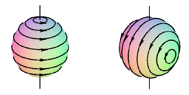
then our perturbed 3-velocity (21) simply becomes,

$$\delta v^{a}=-iKr^{2}\epsilon^{abc}\nabla_{b}Y_{1}^{0}\nabla_{c}r=\hat{\Omega}\varphi^{a},$$ (57)

which represents a small change $\hat{\Omega}$ in the uniform angular velocity $\Omega$ of the star, as claimed. This perturbed velocity field is displayed in Fig. (1).

The case $l=m>0$.

Eqs. (46)-(52) also have a simple solution when $l=m>0$. The Papalouizou and Pringle frequency (52) becomes,

$$\kappa\Omega=(\sigma+m\Omega)=\frac{2\Omega}{(m+1)}.$$ (58)

The definition of $Q_{l}$, Eq. (28), gives,

$$\begin{array}[t]{ccc}Q^{2}_{m}=0,&\mbox{and}&Q^{2}_{m+1}=\displaystyle{\frac{1}{(2m+3)}}.\end{array}$$ (59)

These, again, imply that Eq. (51) is trivially satisfied, while Eqs. (46) and (50) both become,

$$0=U^{\prime}_{m}-\frac{(m+1)}{r}U_{m}$$ (60)

with solution,

$$U_{m}(r)=\left(\frac{r}{R}\right)^{m+1}.$$ (61)

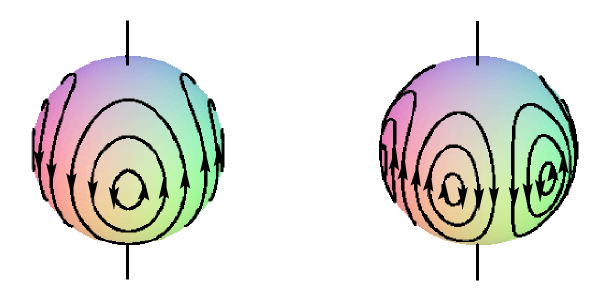
We have chosen the normalization of this solution so that $U_{m}=1$ at the surface of the star, $r=R$. Images of the perturbed velocity field $\delta v^{a}$ for the r-modes with $1\leq l=m\leq 3$ are shown in Fig. (1). We note that the mode with $l=m=1$ has zero-frequency in the inertial frame,

$$\sigma=(\kappa-1)\Omega=0,$$ (62)

and represents rotation of the star about an axis perpendicular to its original axis of rotation. In addition, we note that the r-mode with $l=m=2$ is the one expected to dominate the gravitational radiation driven instability in hot, young neutron stars.

2.4 Numerical Method

In our numerical solution, we restrict consideration to slowly rotating stars, finding axial- and polar-led hybrids to lowest order in the angular velocity $\Omega$. That is, we assume that perturbed quantities introduced above obey the following ordering in $\Omega$:

$$\begin{array}[]{rrrr}W_{l}\sim O(1),&V_{l}\sim O(1),&U_{l}\sim O(1),&\\ \delta\rho\sim O(\Omega),&\delta p\sim O(\Omega),&\delta\Phi\sim O(\Omega),&\sigma\sim O(\Omega).\end{array}$$ (63)

The $\Omega\rightarrow 0$ limit of such a perturbation is a sum of the zero-frequency axial and polar perturbations considered in Sect. 2.2. Note that, although the relative orders of $\delta\rho$ and $\delta v^{a}$ are physically meaningful, there is an arbitrariness in their absolute order. If $(\delta\rho,\delta v^{a})$ is a solution to the linearized equations, so is $(\Omega\delta\rho,\Omega\delta v^{a})$. We have chosen the order (63) to reflect the existence of well-defined, nontrivial velocity perturbations of the spherical model. Other authors (e.g., Lindblom and Ipser [50]) adopt a convention in which $\delta v^{a}=O(\Omega)$ and $\delta\rho=O(\Omega^{2})$.

To lowest order, the equations governing these perturbations are the perturbed Euler equations (42)-(44) and the perturbed mass conservation equation, (6), which becomes

$$rW^{\prime}_{l}+\left(1+r\frac{\rho^{\prime}}{\rho}\right)W_{l}-l(l+1)V_{l}=0.$$ (64)

In addition, the perturbations must satisfy the boundary conditions of regularity at the center of the star, $r=0$, regularity at the surface of the star, $r=R$, and the vanishing of the lagrangian change in the pressure at the surface of the star,

$$0=\Delta p\equiv\delta p+\pounds_{\xi}p=\xi^{r}p^{\prime}+O\mbox{($\Omega$)}.$$ (65)

Equations (42)-(44) and (64) are a system of ordinary differential equations for $W_{l^{\prime}}(r)$, $V_{l^{\prime}}(r)$ and $U_{l^{\prime}}(r)$ (for all $l^{\prime}$). Together with the boundary conditions, these equations form a non-linear eigenvalue problem for the parameter $\kappa$, where $\kappa\Omega$ is the mode frequency in the rotating frame.

To solve for the eigenvalues we proceed as follows. We first ensure that the boundary conditions are automatically satisfied by expanding $W_{l^{\prime}}(r)$, $V_{l^{\prime}}(r)$ and $U_{l^{\prime}}(r)$ (for all $l^{\prime}$) in regular power series about the surface and center of the star. Substituting these series into the differential equations results in a set of algebraic equations for the expansion coefficients. These algebraic equations may be solved for arbitrary values of $\kappa$ using standard matrix inversion methods. For arbitrary values of $\kappa$, however, the series solutions about the center of the star will not agree with those about the surface of the star. The requirement that the series agree at some matching point, $0<r_{0}<R$, then becomes the condition that restricts the possible values of the eigenvalue, $\kappa_{0}$.

The equilibrium solution $(\rho,\Phi)$ appears in the perturbation equations only through the quantity $(\rho^{\prime}/\rho)$ in equation (64). We begin by writing the series expansion for this quantity about $r=0$ as

$$\left(\frac{\rho^{\prime}}{\rho}\right)=\frac{1}{R}\sum^{\infty}_{\stackrel{{\scriptstyle i=1}}{{\mbox{\tiny$i$ odd}}}}\pi_{i}\left(\frac{r}{R}\right)^{i},$$ (66)

and about $r=R$ as

$$\left(\frac{\rho^{\prime}}{\rho}\right)=\frac{1}{R}\sum^{\infty}_{k=-1}\tilde{\pi}_{k}\left(1-\frac{r}{R}\right)^{k},$$ (67)

where the $\pi_{i}$ and $\tilde{\pi}_{k}$ are determined from the equilibrium solution.

Because (42) relates $U_{l}(r)$ algebraically to $W_{l\pm 1}(r)$ and $V_{l\pm 1}(r)$, we may eliminate $U_{l^{\prime}}(r)$ (all $l^{\prime}$) from (43) and (44). We then need only work with one of equations (43) or (44) since the equations (42) through (44) are related by $\nabla_{a}q^{a}=0$.

We next replace $\rho^{\prime}/\rho$, $W_{l^{\prime}}$, and $V_{l^{\prime}}$ in equations (43) or (44) by their series expansions. We eliminate the $U_{l^{\prime}}(r)$ from either (43) or (44) and, again, substitute for the $W_{l^{\prime}}(r)$ and $V_{l^{\prime}}(r)$. Finally, we write down the matching condition at the point $r_{0}$ equating the series expansions about $r=0$ to the series expansions about $r=R$. The result is a linear algebraic system which we may represent schematically as

$$Ax=0.$$ (68)

In this equation, $A$ is a matrix which depends non-linearly on the parameter $\kappa$, and $x$ is a vector whose components are the unknown coefficients in the series expansions for the $W_{l^{\prime}}(r)$ and $V_{l^{\prime}}(r)$. In Appendix B, we explicitly present the equations making up this algebraic system as well as the forms of the regular series expansions for $W_{l^{\prime}}(r)$ and $V_{l^{\prime}}(r)$.

To satisfy equation (68) we must find those values of $\kappa$ for which the matrix $A$ is singular, i.e., we must find the zeroes of the determinant of $A$. We truncate the spherical harmonic expansion of $\delta v^{a}$ at some maximum index $l_{\mbox{\tiny max}}$ and we truncate the radial series expansions about $r=0$ and $r=R$ at some maximum powers $i_{\mbox{\tiny max}}$ and $k_{\mbox{\tiny max}}$, respectively.

The resulting finite matrix is band diagonal. To find the zeroes of its determinant we use standard root finding techniques combined with routines from the LAPACK linear algebra libraries (Anderson et al. [1]). We find that the eigenvalues, $\kappa_{0}$, computed in this manner converge quickly as we increase $l_{\mbox{\tiny max}}$, $i_{\mbox{\tiny max}}$ and $k_{\mbox{\tiny max}}$.

The eigenfunctions associated with these eigenvalues are determined by the perturbation equations only up to normalization. Given a particular eigenvalue, we find its eigenfunction by replacing one of the equations in the system (68) with the normalization condition that

$$\begin{array}[]{ll}V_{m}(r=R)=1&\mbox{for polar-hybrids, or that}\\ V_{m+1}(r=R)=1&\mbox{for axial-hybrids.})\end{array}$$ (69)

Since we have eliminated one of the rows of the singular matrix $A$ in favor of this condition, the result is an algebraic system of the form

$$\tilde{A}x=b,$$ (70)

where $\tilde{A}$ is now a non-singular matrix and $b$ is a known column vector. We solve this system for the vector $x$ using routines from LAPACK and reconstruct the various series expansions from this solution vector of coefficients.

2.5 Eigenvalues and Eigenfunctions

We have computed the eigenvalues and eigenfunctions for uniform density stars and for $n=1$ polytropes, models obeying the polytropic equation of state $p=K\rho^{2}$, where $K$ is a constant. Our numerical solutions for the uniform density star agree with the recent results of Lindblom and Ipser [50] who find analytic solutions for the hybrid modes in rigidly rotating uniform density stars with arbitrary angular velocity - the Maclaurin spheroids. Their calculation uses the two-potential formalism (Ipser and Managan [34]; Ipser and Lindblom [32]) in which the equations for the perturbation modes are reformulated as coupled differential equations for a fluid potential, $\delta U$, and the gravitational potential, $\delta\Phi$. All of the perturbed fluid variables may be expressed in terms of these two potentials. The analysis follows that of Bryan [10] who found that the equations are separable in a non-standard spheroidal coordinate system.

The Bryan/Lindblom-Ipser eigenfunctions $\delta U_{0}$ and $\delta\Phi_{0}$ turn out to be products of associated Legendre polynomials of their coordinates. This simple form of their solutions leads us to expect that our series solutions might also have a simple form - even though their unusual spheroidal coordinates are rather complicated functions of $r$ and $\theta$. In fact, we do find that the modes of the uniform density star have a particularly simple structure. For any particular mode, both the angular and radial series expansions terminate at some finite indices $l_{0}$ and $i_{0}$ (or $k_{0}$). That is, the spherical harmonic expansion (21) of $\delta v^{a}$ contains only terms with $m\leq l\leq l_{0}$ for this mode, and the coefficients of this expansion - the $W_{l}(r)$, $V_{l}(r)$ and $U_{l}(r)$ - are polynomials of order $m+i_{0}$. For all $l_{0}\geq m$ there exist a number of modes terminating at $l_{0}$.

In Tables 1 to 4 we present the functions $W_{l}(r)$, $V_{l}(r)$ and $U_{l}(r)$ for all of the axial- and polar-led hybrids with $m=1$ and $m=2$ for a range of values of the terminating index $l_{0}$. (See also Figure 2.) For given values of $m>0$ and $l_{0}$ there are $l_{0}-m+1$ modes. (When $m=0$ there are $l_{0}$ modes. See Eq. (72) below.) We also find that the last term in the expansion (21), the term with $l=l_{0}$, is always axial for both types of hybrid modes. This fact, together with the fact that the parity of the modes is,

$$\pi=\Biggl{\{}\begin{array}[]{lr}(-1)^{m}&\mbox{for polar-led hybrids\phantom{,}}\\ (-1)^{m+1}&\mbox{for axial-led hybrids,}\end{array}$$ (71)

(for $m>0$) implies that $l_{0}-m+1$ must be even for polar-led modes and odd for axial-led modes.

The fact that the various series terminate at $l_{0}$, $i_{0}$ and $k_{0}$ implies that Equations (68) and (70) will be exact as long as we truncate the series at $l_{\mbox{\tiny max}}\geq l_{0}$, $i_{\mbox{\tiny max}}\geq i_{0}$ and $k_{\mbox{\tiny max}}\geq k_{0}$.

To find the eigenvalues of these modes we search the $\kappa$ axis for all of the zeroes of the determinant of the matrix $A$ in equation (68). We begin by fixing $m$ and performing the search with $l_{\mbox{\tiny max}}=m$. We then increase $l_{\mbox{\tiny max}}$ by 1 and repeat the search (and so on). At any given value of $l_{\mbox{\tiny max}}$, the search finds all of the eigenvalues associated with the eigenfunctions terminating at $l_{0}\leq l_{\mbox{\tiny max}}$.

In Table 5, we present the eigenvalues $\kappa_{0}$ found by this method for the axial- and polar-led hybrid modes of uniform density stars for a range of values of $l_{0}$ and $m$. Observe that many of the eigenvalues, (marked with a $\ast$) satisfy the CFS instability condition $\sigma(\sigma+m\Omega)<0$ (see Sect. 1.1). The modes whose frequencies satisfy this condition are subject to the non-axisymmetric gravitational radiation driven instability in the absence of viscosity. The modes having $l_{0}=m>0$ (or $l_{0}=1$ for $m=0$) are the purely axial r-modes with eigenvalues $\kappa_{0}=2/(m+1)$ (or $\kappa_{0}=0$ for $m=0$) discussed in Sect. 2.3.1. We find that there are no purely polar modes satisfying our assumptions (63) in these stellar models.

We have compared these eigenvalues with those of Lindblom and Ipser [50]. To lowest non-trivial order in $\Omega$ their equation for the eigenvalue, $\kappa_{0}$, can be expressed in terms of associated Legendre polynomials (see Lindblom and Ipser’s equation 6.4), as

$$(4-\kappa_{0}^{2})\frac{d}{d\kappa}P_{l_{0}+1}^{m}(\frac{1}{2}\kappa_{0})-2mP_{l_{0}+1}^{m}(\frac{1}{2}\kappa_{0})=0.$$ (72)

For given values of $m>0$ and $l_{0}$ this equation has $l_{0}-m+1$ roots (corresponding to the number of distinct modes), which can easily be found numerically. (For $m=0$ there are $l_{0}$ roots.) For the range of values of $m$ and $l_{0}$ checked our eigenvalues agree with these to machine precision. (Compare our Table 5 with Table 1 in Lindblom and Ipser [50].)

We have also compared our eigenfunctions with those of Lindblom and Ipser. For a uniformly rotating, isentropic star, the fluid velocity perturbation, $\delta v^{a}$, is related (Ipser and Lindblom [32]) to their fluid potential $\delta U$ by

$$\nabla_{a}\delta U=-\left[i\kappa\Omega g_{ab}+2\nabla_{b}v_{a}\right]\delta v^{b}.$$ (73)

Since the $\varphi$ component of this equation is simply

$$im\delta U=-\Omega r^{2}\sin^{2}\theta\left[\frac{2}{r}\delta v^{r}+2\cot\theta\delta v^{\theta}+i\kappa\delta v^{\varphi}\right],$$ (74)

it is straightforward numerically to construct this quantity from the components of our $\delta v^{a}$ and compare it with the analytic solutions for $\delta U$ given by Lindblom and Ipser (see their Eq. 7.2). We have compared these solutions on a $20\times 40$ grid in the ($r-\theta$) plane and found that they agree (up to normalization) to better than $1$ part in $10^{9}$ for all cases checked.

Because of the use of the two-potential formalism and the unusual coordinate system used in their analysis, the axial- or polar-hybrid character of the Bryan/Lindblom-Ipser solutions is not obvious. Nor is it evident that these solutions have, as their $\Omega\rightarrow 0$ limit, the zero-frequency convective modes described in Sect. 2.2. The comparison of their analytic results with our numerical work has served the dual purpose of clarifying these properties of the solutions and of testing the accuracy of our code. The computational differences are minor between the uniform density calculation and one in which the star obeys a more realistic equation of state. Thus, this testing gives us confidence in the validity of our code for the polytrope calculation. As a further check, we have written two independent codes and compared the eigenvalues computed from each. One of these codes is based on the set of equations described in Appendix B. The other is based on the set of second order equations that results from using the mass conservation equation, (64), to substitute for all the $V_{l}(r)$ in favor of the $W_{l}(r)$.

For the $n=1$ polytrope we will consider and, more generally, for any isentropic equation of state, the purely axial r-modes are independent of the equation of state. In both isentropic and non-isentropic stars, pure r-modes exist whose velocity field is, to lowest order in $\Omega$, an axial vector field belonging to a single angular harmonic (and restricted to harmonics with $l=m$ in the isentropic case). The frequency of such a mode is given (to order $\Omega$) by the Papalouizou and Pringle [60] expression, Eq. (1), and is independent of the equation of state. As we saw in Sect. 2.3.1, only those modes having $l=m$ (or $l=1$ for $m=0$) exist in isentropic stars, and for these modes the eigenfunctions are also independent of the (isentropic) equation of state. This independence of the equation of state occurs for the r-modes because (to lowest order in $\Omega$) fluid elements move in surfaces of constant $r$ (and thus in surfaces of constant density and pressure). For the hybrid modes, however, fluid elements are not confined to surfaces of constant $r$ and one would expect the eigenfrequencies and eigenfunctions to depend on the equation of state.

Indeed, we find such a dependence. The hybrid modes of the $n=1$ polytrope are not identical to those of the uniform density star. On the other hand, the modes do not appear to be very sensitive to the equation of state. We have found that the character of the polytropic modes is similar to the modes of the uniform density star, except that the radial and angular series expansions do not terminate. For each eigenfunction in the uniform density star there is a corresponding eigenfunction in the polytrope with a slightly different eigenfrequency (See Table 6.) For a given mode of the uniform density star, the series expansion (21) terminates at $l=l_{0}$. For the corresponding polytrope mode, the expansion (21) does not terminate, but it does converge quickly. The largest terms in (21) with $l>l_{0}$ are more than an order of magnitude smaller than those with $l\leq l_{0}$ and they decrease rapidly as $l$ increases. Thus, the terms that dominate the polytrope eigenfunctions are those that correspond to the non-zero terms in the corresponding uniform density eigenfunctions.

In Figures 2 and 3 we display the coefficients $W_{l}(r)$, $V_{l}(r)$ and $U_{l}(r)$ of the expansion (21) for the same $m=2$ axial-led hybrid mode in each stellar model. For the uniform density star (Figure 2) the only non-zero coefficients for this mode are those with $l\leq l_{0}=4$. These coefficients are presented explicitly in Table 3 and are low order polynomials in $r$. For the corresponding mode in the polytrope, we present in Figure 3 the first seven coefficients of the expansion (21). Observe that those coefficients with $l\leq 4$ are similar to the corresponding functions in the uniform density mode and dominate the polytrope eigenfunction. The coefficients with $4<l\leq 6$ are an order of magnitude smaller than the dominant coefficients and those with $l>6$ are smaller still. (Since they would be indistinguishable from the $(r/R)$ axis, we do not display the coefficients having $l>6$ for this mode.)

Just as the angular series expansion fails to terminate for the polytrope modes, so too do the radial series expansions for the functions $W_{l}(r)$, $V_{l}(r)$ and $U_{l}(r)$. We have seen that in the uniform density star these functions are polynomials in $r$ (Tables 1 through 4). In the polytropic star, the radial series do not terminate and we are required to work with both sets of radial series expansions - those about the center of the star and those about its surface - in order to represent the functions accurately everywhere inside the star.

In Figures 4 through 12 we compare corresponding functions from each type of star. For example, Figures 4, 5, and 6 show the functions $W_{l}(r)$, $V_{l}(r)$ and $U_{l}(r)$ (respectively) for $l\leq 6$ for a particular $m=1$ polar-led hybrid mode. In the uniform density star this mode has eigenvalue $\kappa_{0}=1.509941$, and in the polytrope it has eigenvalue $\kappa_{0}=1.412999$. The only non-zero functions in the uniform density mode are those with $l\leq l_{0}=2$ and they are simple polynomials in $r$ (see Table 2). Observe that these functions are similar, but not identical to, their counterparts in the polytrope mode, which have been constructed from their radial series expansions about $r=0$ and $r=R$ (with matching point $r_{0}=0.5R$). Again, note the convergence with increasing $l$ of the polytrope eigenfunction. The mode is dominated by the terms with $l\leq 2$ and those with $l>2$ decrease rapidly with $l$. (The $l=5$ and $l=6$ coefficients are virtually indistinguishable from the $(r/R)$ axis.)

Because the polytrope eigenfunctions are dominated by their $l\leq l_{0}$ terms, the eigenvalue search with $l_{\mbox{\tiny max}}=l_{0}$ will find the associated eigenvalues approximately. We compute these approximate eigenvalues of the polytrope modes using the same search technique as for the uniform density star. We then increase $l_{\mbox{\tiny max}}$ and search near one of the approximate eigenvalues for a corrected value, iterating this procedure until the eigenvalue converges to the desired accuracy. We present the eigenvalues found by this method in Table 6.

As a further comparison between the mode eigenvalues in the polytropic star and those in the uniform density star we have modelled a sequence of “intermediate” stars. By multiplying the expansions (66) and (67) for $(\rho^{\prime}/\rho)$ by a scaling factor, $\epsilon\in[0,1]$, we can simulate a continuous sequence of stellar ]models connecting the uniform density star ($\epsilon=0$) to the polytrope ($\epsilon=1$). We find that an eigenvalue in the uniform density star varies smoothly as function of $\epsilon$ to the corresponding eigenvalue in the polytrope.

2.6 Dissipation

The effects of gravitational radiation and viscosity on the pure $l_{0}=m$ r-modes discussed in Sect. 2.3.1 have already been studied by a number of authors. (Lindblom et al. [54], Owen et al. [59], Andersson et al. [3], Kokkotas and Stergioulas [43], Lindblom et al. [53]) All of these modes are unstable to gravitational radiation reaction, and for some of them this instability strongly dominates viscous damping. We now consider the effects of dissipation on the axial- and polar-hybrid modes.

To estimate the timescales associated with viscous damping and gravitational radiation reaction we follow the methods used for the $l_{0}=m$ modes (Lindblom et al. [54], see also Ipser and Lindblom [33]). When the energy radiated per cycle is small compared to the energy of the mode, the imaginary part of the mode frequency is accurately approximated by the expression

$$\frac{1}{\tau}=-\frac{1}{2E}\frac{dE}{dt},$$ (75)

where $E$ is the energy of the mode as measured in the rotating frame,

$$E=\frac{1}{2}\int\left[\rho\delta v^{a}\delta v^{\ast}_{a}+\left(\frac{\delta p}{\rho}+\delta\Phi\right)\delta\rho^{\ast}\right]d^{3}x.$$ (76)

The rate of change of this energy due to dissipation by viscosity and gravitational radiation is,

$$\frac{dE}{dt} = -\int\left(2\eta\delta\sigma^{ab}\delta\sigma_{ab}^{\ast}+\zeta\delta\theta\delta\theta^{\ast}\right)$$ (77)

$$-\sigma(\sigma+m\Omega)\sum_{l\geq 2}N_{l}\sigma^{2l}\left(\left|\delta D_{lm}\right|^{2}+\left|\delta J_{lm}\right|^{2}\right).$$

The first term in (77) represents dissipation due to shear viscosity, where the shear, $\delta\sigma_{ab}$, of the perturbation is

$$\delta\sigma_{ab}=\frac{1}{2}\left(\nabla_{a}\delta v_{b}+\nabla_{b}\delta v_{a}-\frac{2}{3}g_{ab}\nabla_{c}\delta v^{c}\right),$$ (78)

and the coefficient of shear viscosity for hot neutron-star matter is (Cutler and Lindblom [17]; Sawyer [68])

$$\eta=2\times 10^{18}\left(\frac{\rho}{10^{15}\mbox{g}\!\cdot\!\mbox{cm}^{-3}}\right)^{\frac{9}{4}}\left(\frac{10^{9}K}{T}\right)^{2}\ \mbox{g}\!\cdot\!\mbox{cm}^{-1}\!\cdot\!\mbox{s}^{-1}.$$ (79)

The second term in (77) represents dissipation due to bulk viscosity, where the expansion, $\delta\theta$, of the perturbation is

$$\delta\theta=\nabla_{c}\delta v^{c}$$ (80)

and the bulk viscosity coefficient for hot neutron star matter is (Cutler and Lindblom [17]; Sawyer [68])

$$\zeta=6\times 10^{25}\left(\frac{1\mbox{Hz}}{\sigma+m\Omega}\right)^{2}\left(\frac{\rho}{10^{15}\mbox{g}\!\cdot\!\mbox{cm}^{-3}}\right)^{2}\left(\frac{T}{10^{9}K}\right)^{6}\ \mbox{g}\!\cdot\!\mbox{cm}^{-1}\!\cdot\!\mbox{s}^{-1}.$$ (81)

The third term in (77) represents dissipation due to gravitational radiation, with coupling constant

$$N_{l}=\frac{4\pi G}{c^{2l+1}}\frac{(l+1)(l+2)}{l(l-1)[(2l+1)!!]^{2}}.$$ (82)

The mass, $\delta D_{lm}$, and current, $\delta J_{lm}$, multipole moments of the perturbation are given by (Thorne [78], Lindblom et al. [54])

$$\delta D_{lm}=\int\delta\rho r^{l}Y_{l}^{\ast m}d^{3}x,$$ (83)

and

$$\delta J_{lm}=\frac{2}{c}\left(\frac{l}{l+1}\right)^{\frac{1}{2}}\int r^{l}\left(\rho\delta v_{a}+\delta\rho v_{a}\right)Y^{a,B\ast}_{lm}d^{3}x$$ (84)

where $Y^{a,B}_{lm}$ is the magnetic type vector spherical harmonic (Thorne [78]) given by,

$$Y^{a,B}_{lm}=-\frac{r}{\sqrt{l(l+1)}}\epsilon^{abc}\nabla_{b}Y_{l}^{m}\nabla_{c}r.$$ (85)

To lowest order in $\Omega$, the energy (76) of the hybrid modes is positive definite. Their stability is therefore determined by the sign of the right hand side of equation (77). We have seen that many of the hybrid modes have frequencies satisfying the CFS instability criterion $\sigma(\sigma+m\Omega)<0$. It is now clear that this makes the third term in Eq. (77) positive, implying that gravitational radiation reaction tends to drive these modes unstable. As discussed in Sect. 1.1, however, to determine the actual stability of these modes, we must evaluate the various dissipative terms in (77).

We first substitute for $\delta v^{a}$ the spherical harmonic expansion (21) and use the orthogonality relations for vector spherical harmonics (Thorne [78]) to perform the angular integrals. The energy of the modes in the rotating frame then becomes

$$E=\sum^{\infty}_{l=m}\frac{1}{2}\int_{0}^{R}\rho\left[W_{l}^{2}+l(l+1)V_{l}^{2}+l(l+1)U_{l}^{2}\right]dr.$$ (86)

To calculate the dissipation due to gravitational radiation reaction we must evaluate the multipole moments (83) and (84). To lowest order in $\Omega$ the mass multipole moments (83) vanish and the current multipole moments are given by

$$\delta J_{lm}=\frac{2il}{c}\int_{0}^{R}\rho r^{l+1}U_{l}dr.$$ (87)

To calculate the dissipation due to bulk viscosity we must evaluate the expansion, $\delta\theta=\nabla_{c}\delta v^{c}$, of the perturbation. For uniform density stars this quantity vanishes identically by the mass conservation equation (6). For the $l_{0}=m$, pure axial modes the expansion, again, vanishes identically, regardless of the equation of state. To compute the bulk viscosity of these modes it is necessary to work to higher order in $\Omega$ (Andersson et al. [3], Lindblom et al. [53]). On the other hand, for the new hybrid modes in which we are interested, the expansion of the fluid perturbation is non-zero in the slowly rotating polytropic stars. After substituting for $\delta v^{a}$ its series expansion and performing the angular integrals, the bulk viscosity contribution to (77) becomes

$$\left(\frac{dE}{dt}\right)_{B}=-\sum^{\infty}_{l=m}\int_{0}^{R}\frac{\zeta}{r^{2}}\left[rW^{\prime}_{l}+W_{l}-l(l+1)V_{l}\right]^{2}dr$$ (88)

In a similar manner, the contribution to (77) from shear viscosity becomes

$$\left(\frac{dE}{dt}\right)_{S}=-\sum^{\infty}_{l=m}\int_{0}^{R}\begin{array}[t]{l}\displaystyle{\frac{2\eta}{r^{2}}}\Biggl{\{}\displaystyle{\frac{2}{3}\left[r^{3}\left(\frac{W_{l}}{r^{2}}\right)^{\prime}\right]^{2}+\frac{1}{2}l(l+1)W_{l}^{2}}\\ \\ +\displaystyle{\frac{1}{2}l(l+1)\left[r^{3}\left(\frac{V_{l}}{r^{2}}\right)^{\prime}\right]^{2}+\frac{1}{3}l(l+1)(2l^{2}+2l-3)V_{l}^{2}}\\ \\ +\displaystyle{l(l+1)W_{l}\left[r^{5}\left(\frac{V_{l}}{r^{4}}\right)^{\prime}\right]+\frac{2}{3}l(l+1)V_{l}\left(rW_{l}\right)^{\prime}}\\ \\ +\displaystyle{\frac{1}{2}l(l+1)\left[r^{3}\left(\frac{U_{l}}{r^{2}}\right)^{\prime}\right]^{2}+\frac{1}{2}l(l+1)(l^{2}+l-2)U_{l}^{2}}\Biggr{\}}dr.\end{array}$$ (89)

Given a numerical solution for one of the hybrid mode eigenfunctions, these radial integrals can be performed numerically. The resulting contributions to (77) also depend on the angular velocity and temperature of the star. Let us express the imaginary part of the hybrid mode frequency (75) as,

$$\frac{1}{\tau}=\frac{1}{\tilde{\tau}_{S}}\left(\frac{10^{9}K}{T}\right)^{2}+\frac{1}{\tilde{\tau}_{B}}\left(\frac{T}{10^{9}K}\right)^{6}\left(\frac{\pi G\bar{\rho}}{\Omega^{2}}\right)+\sum_{l\geq 2}\frac{1}{\tilde{\tau}_{l}}\left(\frac{\Omega^{2}}{\pi G\bar{\rho}}\right)^{l+1},$$ (90)

where $\bar{\rho}$ is average density of the star. (Compare this expression to the corresponding expression in Lindblom et al. [54] - their equation (22) - for the $l_{0}=m$ pure axial modes.)

The bulk viscosity term in this equation is stronger by a factor $\Omega^{-4}$ than that for the $l_{0}=m$ pure axial modes. This is because the expansion $\delta\theta$ of the hybrid mode is nonzero to lowest order in $\Omega$ for the polytropic star, whereas it is order $\Omega^{2}$ for the pure axial modes. This implies that the damping due to bulk viscosity will be much stronger for the hybrid modes than for the pure axial modes in slowly rotating stars.

Note that the contribution to (90) from gravitational radiation reaction consists of a sum over all the values of $l$ with a non-vanishing current multipole. This sum is, of course, dominated by the lowest contributing multipole.

In Tables 7 to 9 we present the timescales for these various dissipative effects in the uniform density and polytropic stellar models that we have been considering with $R=12.57\mbox{km}$ and $M=1.4M_{\odot}$. For the reasons discussed above, we do not present bulk viscosity timescales for the uniform density star.

Given the form of their eigenfunctions, it seems reasonable to expect that some of the unstable hybrid modes might grow on a timescale which is comparable to that of the pure $l_{0}=m$ r-modes. For example, the $m=2$ axial-led hybrids all have $U_{2}(r)\neq 0$ (see, for example, Figures 2 and 3). By equation (87), this leads one to expect a non-zero current quadrupole moment $\delta J_{22}$, and this is the multipole moment that dominates the gravitational radiation in the r-modes. Upon closer inspection, however, one finds that this is not the case. In fact, we find that all of the multipoles $\delta J_{lm}$ vanish (or nearly vanish) for $l<l_{0}$, where $l_{0}$ is the largest value of $l$ contributing a dominant term to the expansion (21) of $\delta v^{a}$.

In the uniform density star, these multipoles vanish identically. Consider, for example, the $m=2$, $l_{0}=4$ axial-hybrid with eigenvalue $\kappa=0.466901$. (See Table 3 and Figure 7) For this mode, $U_{2}\propto(7x^{3}-9x^{5})$, where $x=(r/R)$. By equation (87), we then find that

$$\delta J_{22}\propto\int_{0}^{1}x^{3}(7x^{3}-9x^{5})dx\equiv 0,$$ (91)

and that $\delta J_{42}$ is the only non-zero radiation multipole. In general, the only non-zero multipole for an axial- or polar-hybrid mode in the uniform density star is $\delta J_{l_{0}\,m}$.

That this should be the case is not obvious from the form of our eigenfunctions. However, Lindblom and Ipser’s [50] analytic solutions provide an explanation. Their equations (7.1) and (7.3) reveal that the perturbed gravitational potential, $\delta\Phi$, is a pure spherical harmonic to lowest order in $\Omega$. In particular,

$$\delta\Phi\propto Y_{l_{0}+1}^{m}.$$ (92)

This implies that the only non-zero current multipole is $\delta J_{l_{0}\,m}$.

We find a similar result for the polytropic star. Because of the similarity between the modes in the polytrope and the modes in the uniform density star, we find that although the lower $l$ current multipoles do not vanish identically, they very nearly vanish and the radiation is dominated by higher $l$ multipoles.

The fastest growth times we find in the hybrid modes are of order $10^{4}$ seconds (at $10^{9}K$ and $\Omega=\sqrt{\pi G\bar{\rho}}$). Thus, the spin-down of a newly formed neutron star will be dominated by the $l_{0}=m=2$ mode with small contributions from the $l_{0}=m$ pure axial modes with $2\leq m\mathrel{\mathchoice{\vbox{\offinterlineskip\halign{\hfil$\displaystyle#$\hfil\cr<\cr\sim\cr}}}{\vbox{\offinterlineskip\halign{\hfil$\textstyle#$\hfil\cr<\cr\sim\cr}}}{\vbox{\offinterlineskip\halign{\hfil$\scriptstyle#$\hfil\cr<\cr\sim\cr}}}{\vbox{\offinterlineskip\halign{\hfil$\scriptscriptstyle#$\hfil\cr<\cr\sim\cr}}}}10$ and from the fastest growing hybrid modes.

Table 1: Axial-Hybrid Eigenfunctions with $m=1$ for Uniform Density Stars.

Table 2: Polar-Hybrid Eigenfunctions with $m=1$ for Uniform Density Stars.

Table 3: Axial-Hybrid Eigenfunctions with $m=2$ for Uniform Density Stars.

Table 4: Polar-Hybrid Eigenfunctions with $m=2$ for Uniform Density Stars.

Table 5: Eigenvalues $\kappa_{0}$ for Uniform Density Stars.

Table 6: Eigenvalues $\kappa_{0}$ for the $p=K\rho^{2}$ Polytrope.

Table 7: Dissipative timescales (in seconds) for $m=1$ axial-hybrid modes at $T=10^{9}K$ and $\Omega=\sqrt{\pi G\bar{\rho}}$.

Table 8: Dissipative timescales (in seconds) for $m=2$ axial-hybrid modes at $T=10^{9}K$ and $\Omega=\sqrt{\pi G\bar{\rho}}$.

Table 9: Dissipative timescales (in seconds) for $m=2$ polar-hybrid modes at $T=10^{9}K$ and $\Omega=\sqrt{\pi G\bar{\rho}}$.

123456789012345$l=1$		$l=1$
123456789012345$m=0$		$m=1$

123456789012345$l=2$		$l=3$
123456789012345$m=2$		$m=3$

Figure 1: Images of the perturbed velocity field $\delta v^{a}$ for a few of the newtonian r-modes at a fixed time. The velocity profile shown rotates forward in the inertial frame with angular velocity $(l-1)(l+2)\Omega/l(l+1)$ and backward in the rotating frame with angular velocity $2\Omega/l(l+1)$. Fluid elements oscillate in small circles in the rotating frame as their velocity changes in accordance with this rotating profile.

Figure 2: All of the non-zero coefficients $W_{l}(r)$, $V_{l}(r)$, $U_{l}(r)$ of the spherical harmonic expansion (21) for a particular $m=2$ axial-led hybrid mode of the uniform density star. The mode has eigenvalue $\kappa_{0}=-0.763337$. Note that the largest value of $l$ that appears in the expansion (21) is $l_{0}=4$ and that the functions $W_{l}(r)$, $V_{l}(r)$ and $U_{l}(r)$ are low order polynomials in $(r/R)$. (See Table 3.) The mode is normalized so that $V_{3}(r=R)=1$.

Figure 3: The coefficients $W_{l}(r)$, $V_{l}(r)$, $U_{l}(r)$ with $l\leq 6$ of the spherical harmonic expansion (21) for a particular $m=2$ axial-led hybrid mode of the polytropic star. This is the polytrope mode that corresponds to the uniform density mode displayed in Figure 2. For the polytrope the mode has eigenvalue $\kappa_{0}=-1.025883$. The expansion (21) converges rapidly with increasing $l$ and is dominated by the terms with $2\leq l\leq 4$, i.e., by the terms corresponding to those which are non-zero for the uniform density mode. Observe that the coefficients shown with $4<l\leq 6$ are an order of magnitude smaller than those with $2\leq l\leq 4$. Those with $l>6$ are smaller still and are not displayed here. The mode is, again, normalized so that $V_{3}(r=R)=1$.

Figure 4: The functions $W_{l}(r)$ with $l\leq 6$ for a particular $m=1$ polar-led hybrid mode. For the uniform density star this mode has eigenvalue $\kappa_{0}=1.509941$ and $W_{1}=-x+x^{3}$ ($x=r/R$) is the only non-vanishing $W_{l}(r)$ (see Table 2). The corresponding mode of the polytropic star has eigenvalue $\kappa_{0}=1.412999$. Observe that $W_{1}(r)$ for the polytrope, which has been constructed from its power series expansions about $r=0$ and $r=R$, is similar, though not identical, to the corresponding $W_{1}(r)$ for the uniform density star. Observe also that the functions $W_{l}(r)$ with $l>1$ for the polytrope are more than an order of magnitude smaller than $W_{1}(r)$ and become smaller with increasing $l$. ($W_{5}(r)$ is virtually indistinguishable from the $(r/R)$ axis.)

Figure 5: The functions $V_{l}(r)$ with $l\leq 6$ for the same mode as in Figure 4.

Figure 6: The functions $U_{l}(r)$ with $l\leq 6$ for the same mode as in Figure 4.

Figure 7: The functions $U_{l}(r)$ with $l\leq 7$ for a particular $m=2$ axial-led hybrid mode. For the uniform density star this mode has eigenvalue $\kappa_{0}=0.466901$ and $U_{2}(r)$ and $U_{4}(r)$ are the only non-vanishing $U_{l}(r)$. (See Table 3 for their explicit forms.) The corresponding mode of the polytropic star has eigenvalue $\kappa_{0}=0.517337$. Observe that $U_{2}(r)$ and $U_{4}(r)$ for the polytrope, which have been constructed from their power series expansions about $r=0$ and $r=R$, are similar, though not identical, to the corresponding functions for the uniform density star. Observe also that $U_{6}(r)$ is more than an order of magnitude smaller than $U_{2}(r)$ and $U_{4}(r)$.

Figure 8: The functions $W_{l}(r)$ with $l\leq 7$ for the same mode as in Figure 7.

Figure 9: The functions $V_{l}(r)$ with $l\leq 7$ for the same mode as in Figure 7.

Figure 10: The functions $U_{l}(r)$ with $l\leq 8$ for a particular $m=2$ axial-led hybrid mode. For the uniform density star this mode has eigenvalue $\kappa_{0}=0.359536$ and $U_{2}(r)$, $U_{4}(r)$ and $U_{6}(r)$ are the only non-vanishing $U_{l}(r)$. (See Table 3 for their explicit forms.) The corresponding mode of the polytropic star has eigenvalue $\kappa_{0}=0.421678$. Observe that $U_{2}(r)$, $U_{4}(r)$ and $U_{6}(r)$ for the polytrope, which have been constructed from their power series expansions about $r=0$ and $r=R$, are similar, though not identical, to the corresponding functions for the uniform density star. Observe also that $U_{8}(r)$ is more than an order of magnitude smaller than $U_{2}(r)$, $U_{4}(r)$ and $U_{6}(r)$.

Figure 11: The functions $W_{l}(r)$ with $l\leq 8$ for the same mode as in Figure 10.

Figure 12: The functions $V_{l}(r)$ with $l\leq 8$ for the same mode as in Figure 10.

Chapter 3 Relativistic Stars: Analytic Results

In Ch. 2 we examined the rotationally restored hybrid modes of isentropic newtonian stars. We now consider the corresponding modes in relativistic stars. As in the newtonian case, we must begin by examining the perturbations of the non-rotating star, and finding all of the modes belonging to its degenerate zero-frequency subspace.

3.1 Stationary Perturbations of Spherical Stars

The equilibrium of a spherical perfect fluid star is described by a static, spherically symmetric spacetime with metric $g_{\alpha\beta}$ of the form,

$$ds^{2}=-e^{2\nu(r)}dt^{2}+e^{2\lambda(r)}dr^{2}+r^{2}d\theta^{2}+r^{2}sin^{2}\theta d\varphi^{2},$$ (1)

and with energy-momentum tensor,

$$T_{\alpha\beta}=(\epsilon+p)u_{\alpha}u_{\beta}+pg_{\alpha\beta},$$ (2)

where $\epsilon(r)$ is the total fluid energy density, $p(r)$ is the fluid pressure and

$$u^{\alpha}=e^{-\nu}t^{\alpha}$$ (3)

is the fluid 4-velocity - with $t^{\alpha}=(\partial_{t})^{\alpha}$ the timelike Killing vector of the spacetime.

These satisfy an equation of state of the form

$$p=p(\epsilon)$$ (4)

as well as the Einstein equations, $G_{\alpha\beta}=8\pi T_{\alpha\beta}$, which are equivalent to

$$\frac{dp}{dr}=-\frac{(\epsilon+p)(M+4\pi r^{3}p)}{r(r-2M)},$$ (5)

$$\frac{dM}{dr}=4\pi r^{2}\epsilon$$ (6)

and

$$\frac{d\nu}{dr}=-\frac{1}{(\epsilon+p)}\frac{dp}{dr}$$ (7)

where

$$M(r)\equiv\frac{1}{2}r(1-e^{-2\lambda}).$$ (8)

(See, e.g., Wald [82], Ch.6.)

We are, again, interested in the space of zero-frequency modes, the linearized, time-independent perturbations of this static equilibrium. As in the newtonian case, we find that this zero-frequency subspace is spanned by two classes of perturbations. To identify these classes explicitly, we must examine the equations governing the perturbed configuration.

Writing the change in the metric as $h_{\alpha\beta}\equiv\delta g_{\alpha\beta}$, we express the perturbed configuration in terms of the set $(h_{\alpha\beta},\delta u^{\alpha},\delta\epsilon,\delta p)$. These must satisfy the perturbed Einstein equations $\delta G_{\alpha}^{\ \beta}=8\pi\delta T_{\alpha}^{\ \beta}$, together with an equation of state (which may, in general, differ from that of the equilibrium configuration).

The perturbed Einstein tensor is given by

$$\delta G_{\alpha}^{\ \beta}=-\frac{1}{2}\biggl{\{}\begin{array}[t]{l}\nabla_{\gamma}\nabla^{\gamma}h_{\alpha}^{\ \beta}-\nabla_{\gamma}\nabla^{\beta}h_{\alpha}^{\ \gamma}-\nabla^{\gamma}\nabla_{\alpha}h_{\gamma}^{\ \beta}+\nabla_{\alpha}\nabla^{\beta}h\\ \\ +2R_{\alpha}^{\ \gamma}h_{\gamma}^{\ \beta}+(\nabla^{\alpha}\nabla^{\beta}h_{\alpha\beta}-\nabla_{\gamma}\nabla^{\gamma}h-R^{\alpha\beta}h_{\alpha\beta})g_{\alpha}^{\ \beta}\biggr{\}}\end{array}$$ (9)

where $h\equiv h_{\alpha}^{\ \alpha}$, $\nabla_{\alpha}$ is the covariant derivative associated with the equilibrium metric and

$$R_{\alpha}^{\ \beta}=8\pi(T_{\alpha}^{\ \beta}-\frac{1}{2}Tg_{\alpha}^{\ \beta})=8\pi\left[(\epsilon+p)u_{\alpha}u^{\beta}+\frac{1}{2}(\epsilon-p)g_{\alpha}^{\ \beta}\right]$$ (10)

is the equilibrium Ricci tensor. The perturbed energy-momentum tensor is given by

$$\delta T_{\alpha}^{\ \beta}=(\delta\epsilon+\delta p)u_{\alpha}u^{\beta}+\delta p\delta_{\alpha}^{\ \beta}+(\epsilon+p)\delta u_{\alpha}u^{\beta}+(\epsilon+p)u_{\alpha}\delta u^{\beta}.$$ (11)

Following Thorne and Campolattaro [79], we expand our perturbed variables in scalar, vector and tensor spherical harmonics. The perturbed energy density and pressure are scalars and therefore must have polar parity, $(-1)^{l}$.

$$\delta\epsilon=\delta\epsilon(r)Y_{l}^{m},$$ (12)

$$\delta p=\delta p(r)Y_{l}^{m}.$$ (13)

The perturbed 4-velocity for a polar-parity mode can be written

$$\delta u_{P}^{\alpha}=\biggl{\{}\frac{1}{2}H_{0}(r)Y_{l}^{m}t^{\alpha}+\frac{1}{r}W(r)Y_{l}^{m}r^{\alpha}+V(r)\nabla^{\alpha}Y_{l}^{m}\biggr{\}}e^{-\nu}$$ (14)

while that of an axial-parity mode can be written

$$\delta u_{A}^{\alpha}=-U(r)e^{(\lambda-\nu)}\epsilon^{\alpha\beta\gamma\delta}\nabla_{\beta}Y_{l}^{m}u_{\gamma}\nabla_{\delta}\,r.$$ (15)

(We have chosen the exact form of these expressions for later convenience.)

To simplify the form of the metric perturbation we will, again, follow Thorne and Campolattaro [79] and work in the Regge-Wheeler [65] gauge. The metric perturbation for a polar-parity mode can be written

$$h_{\mu\nu}^{P}=\left[\begin{array}[c]{cccc}H_{0}(r)e^{2\nu}&H_{1}(r)&0&0\\ H_{1}(r)&H_{2}(r)e^{2\lambda}&0&0\\ 0&0&r^{2}K(r)&0\\ 0&0&0&r^{2}sin^{2}\theta K(r)\end{array}\right]Y_{l}^{m},$$ (16)

while that of an axial-parity mode can be written

$$h_{\mu\nu}^{A}=\left[\begin{array}[c]{cccc}0&0&h_{0}(r)\,(\frac{-1}{sin\theta})\partial_{\varphi}Y_{l}^{m}&h_{0}(r)\,\sin\theta\partial_{\theta}Y_{l}^{m}\\ 0&0&h_{1}(r)\,(\frac{-1}{sin\theta})\partial_{\varphi}Y_{l}^{m}&h_{1}(r)\,\sin\theta\partial_{\theta}Y_{l}^{m}\\ \mbox{\scriptsize symm}&\mbox{\scriptsize symm}&0&0\\ \mbox{\scriptsize symm}&\mbox{\scriptsize symm}&0&0\\ \end{array}\right]$$ (17)

The Regge-Wheeler gauge is unique for perturbations having spherical harmonic index $l\geq 2$. However, when $l=1$ or $l=0$, there remain additional gauge degrees of freedom. In addition, the components of the perturbed Einstein equation acquire a slightly different form in each of these three cases (cf. Campolattaro and Thorne [11]) and will be presented separately below.

We have derived these components using the Maple tensor package by substituting expressions (12)-(17) into Eqs. (9) and (11) (making liberal use of the equilibrium equations (5) through (8) to simplify the resulting expressions). The resulting set of equations for the case $l\geq 2$ are equivalent to those presented in Thorne and Campolattaro [79] upon specializing their equations to the case of stationary perturbations and making the necessary changes of notation. Similarly, the set of equations for the case $l=1$ are equivalent to those presented in Campolattaro and Thorne [11].

3.1.1 The case $l\geq 2$

The non-vanishing components of the perturbed Einstein equation for $l\geq 2$ are as follows. We will use Eq. (21) below, to replace $H_{2}$ by $H_{0}$. From $\delta G_{t}^{\ t}=8\pi\delta T_{t}^{\ t}$ we have

$$0 = e^{-2\lambda}r^{2}K^{\prime\prime}+e^{-2\lambda}(3-r\lambda^{\prime})rK^{\prime}-\left[\frac{1}{2}l(l+1)-1\right]K$$ (18)

$$-e^{-2\lambda}rH_{0}^{\prime}-\left[\frac{1}{2}l(l+1)+1-8\pi r^{2}\epsilon\right]H_{0}+8\pi r^{2}\delta\epsilon.$$

From $\delta G_{r}^{\ r}=8\pi\delta T_{r}^{\ r}$ we similarly have

$$0 = e^{-2\lambda}(1+r\nu^{\prime})rK^{\prime}-\left[\frac{1}{2}l(l+1)-1\right]K$$ (19)

$$-e^{-2\lambda}rH_{0}^{\prime}+\left[\frac{1}{2}l(l+1)-1-8\pi r^{2}p\right]H_{0}-8\pi r^{2}\delta p.$$

From $\delta G_{\theta}^{\ \theta}+\delta G_{\varphi}^{\ \varphi}=8\pi\left(\delta T_{\theta}^{\ \theta}+\delta T_{\varphi}^{\ \varphi}\right)$ we have

$$0 = e^{-2\lambda}r^{2}K^{\prime\prime}+e^{-2\lambda}\left[r(\nu^{\prime}-\lambda^{\prime})+2\right]rK^{\prime}-16\pi r^{2}\delta p$$ (20)

$$-e^{-2\lambda}r^{2}H_{0}^{\prime\prime}-e^{-2\lambda}(3r\nu^{\prime}-r\lambda^{\prime}+2)rH_{0}^{\prime}-16\pi r^{2}pH_{0}.$$

From $\delta G_{\theta}^{\ \theta}-\delta G_{\varphi}^{\ \varphi}=8\pi\left(\delta T_{\theta}^{\ \theta}-\delta T_{\varphi}^{\ \varphi}\right)$ we have

$$H_{2}=H_{0}.$$ (21)

From $\delta G_{r}^{\ \theta}=8\pi\delta T_{r}^{\ \theta}$ we have

$$K^{\prime}=e^{-2\nu}\left[e^{2\nu}H_{0}\right]^{\prime}.$$ (22)

From $\delta G_{t}^{\ r}=8\pi\delta T_{t}^{\ r}$ we have

$$0=H_{1}+\frac{16\pi(\epsilon+p)}{l(l+1)}e^{2\lambda}rW.$$ (23)

From $\delta G_{t}^{\ \theta}=8\pi\delta T_{t}^{\ \theta}$ we have

$$0=e^{-(\nu-\lambda)}\left[e^{(\nu-\lambda)}H_{1}\right]^{\prime}+16\pi(\epsilon+p)e^{2\lambda}V.$$ (24)

From $\delta G_{t}^{\ \varphi}=8\pi\delta T_{t}^{\ \varphi}$ we have

$$h_{0}^{{}^{\prime\prime}}-(\nu^{\prime}+\lambda^{\prime})h_{0}^{\prime}+\left[\frac{(2-l^{2}-l)}{r^{2}}e^{2\lambda}-\frac{2}{r}(\nu^{\prime}+\lambda^{\prime})-\frac{2}{r^{2}}\right]h_{0}=\frac{4}{r}(\nu^{\prime}+\lambda^{\prime})U.$$ (25)

From $\delta G_{r}^{\ \varphi}=8\pi\delta T_{r}^{\ \varphi}$ we have

$$(l-1)(l+2)h_{1}=0.$$ (26)

Finally, from $\delta G_{\theta}^{\ \varphi}=8\pi\delta T_{\theta}^{\ \varphi}$ we have

$$e^{-(\nu-\lambda)}\left[e^{(\nu-\lambda)}h_{1}\right]^{\prime}=0.$$ (27)

3.1.2 The case $l=1$

The $l=1$ case differs from $l\geq 2$ in two respects (Campolattaro and Thorne [11]). Firstly, $H_{2}(r)\neq H_{0}(r)$, because the equation $\delta G_{\theta}^{\ \theta}-\delta G_{\varphi}^{\ \varphi}=8\pi\left(\delta T_{\theta}^{\ \theta}-\delta T_{\varphi}^{\ \varphi}\right)$ vanishes identically. Secondly, we may exploit the aforementioned gauge freedom for this case to eliminate the metric functions $K(r)$ and $h_{1}(r)$. (We note that Eq.(26) implies $h_{1}(r)=0$ for $l\geq 2$ anyway.) With these two differences taken into account the non-vanishing components of the perturbed Einstein equation for $l=1$ are as follows. From $\delta G_{t}^{\ t}=8\pi\delta T_{t}^{\ t}$ we have

$$0=e^{-2\lambda}rH_{2}^{\prime}+\left(2-8\pi r^{2}\epsilon\right)H_{2}-8\pi r^{2}\delta\epsilon.$$ (28)

From $\delta G_{r}^{\ r}=8\pi\delta T_{r}^{\ r}$ we have

$$0=e^{-2\lambda}rH_{0}^{\prime}-H_{0}+\left(1+8\pi r^{2}p\right)H_{2}+8\pi r^{2}\delta p.$$ (29)

From $\delta G_{\theta}^{\ \theta}+\delta G_{\varphi}^{\ \varphi}=8\pi\left(\delta T_{\theta}^{\ \theta}+\delta T_{\varphi}^{\ \varphi}\right)$ we have

$$0 = e^{-2\lambda}r^{2}H_{0}^{\prime\prime}+e^{-2\lambda}(2r\nu^{\prime}-r\lambda^{\prime}+1)rH_{0}^{\prime}-H_{0}$$ (30)

$$+e^{-2\lambda}(1+r\nu^{\prime})rH_{2}^{\prime}+(1+16\pi r^{2}p)H_{2}+16\pi r^{2}\delta p$$

From $\delta G_{r}^{\ \theta}=8\pi\delta T_{r}^{\ \theta}$ we have

$$0=rH_{0}^{\prime}+(r\nu^{\prime}-1)H_{0}+(r\nu^{\prime}+1)H_{2}$$ (31)

From $\delta G_{t}^{\ r}=8\pi\delta T_{t}^{\ r}$ we, again, have

$$0=H_{1}+8\pi(\epsilon+p)e^{2\lambda}rW.$$ (32)

From $\delta G_{t}^{\ \theta}=8\pi\delta T_{t}^{\ \theta}$ we, again, have

$$0=e^{-(\nu-\lambda)}\left[e^{(\nu-\lambda)}H_{1}\right]^{\prime}+16\pi(\epsilon+p)e^{2\lambda}V.$$ (33)

Finally, from $\delta G_{t}^{\ \varphi}=8\pi\delta T_{t}^{\ \varphi}$ we have

$$h_{0}^{{}^{\prime\prime}}-(\nu^{\prime}+\lambda^{\prime})h_{0}^{\prime}-\left[\frac{2}{r}(\nu^{\prime}+\lambda^{\prime})+\frac{2}{r^{2}}\right]h_{0}=\frac{4}{r}(\nu^{\prime}+\lambda^{\prime})U.$$ (34)

3.1.3 The case $l=0$

The $l=0$ case differs yet again from the previous two, being the case of stationary, spherically symmetric perturbations of a static, spherical equilibrium. To maximize the similarity to the preceding two cases we will use the same form for the perturbed metric except that we may now exploit the gauge freedom for this case to eliminate the functions $K(r)$, $H_{1}(r)$ and $h_{1}(r)$. The non-vanishing components of the perturbed Einstein equation for $l=0$ are as follows. From $\delta G_{t}^{\ t}=8\pi\delta T_{t}^{\ t}$ we have

$$0=e^{-2\lambda}rH_{2}^{\prime}+\left(1-8\pi r^{2}\epsilon\right)H_{2}-8\pi r^{2}\delta\epsilon.$$ (35)

From $\delta G_{r}^{\ r}=8\pi\delta T_{r}^{\ r}$ we have

$$0=e^{-2\lambda}rH_{0}^{\prime}+\left(1+8\pi r^{2}p\right)H_{2}+8\pi r^{2}\delta p.$$ (36)

From $\delta G_{\theta}^{\ \theta}+\delta G_{\varphi}^{\ \varphi}=8\pi\left(\delta T_{\theta}^{\ \theta}+\delta T_{\varphi}^{\ \varphi}\right)$ we have

$$0 = e^{-2\lambda}r^{2}H_{0}^{\prime\prime}+e^{-2\lambda}(2r\nu^{\prime}-r\lambda^{\prime}+1)rH_{0}^{\prime}$$ (37)

$$+e^{-2\lambda}(1+r\nu^{\prime})rH_{2}^{\prime}+16\pi r^{2}pH_{2}+16\pi r^{2}\delta p$$

Finally, from $\delta G_{t}^{\ r}=8\pi\delta T_{t}^{\ r}$ we have

$$0=16\pi(\epsilon+p)W.$$ (38)

3.1.4 Decomposition of the zero-frequency subspace.

By inspection of the above three sets of equations, it is evident that they decouple into two independent classes. For $l\geq 2$ Eqs. (18)-(22) involve only the variables $(H_{0},H_{2},K,\delta\epsilon,\delta p)$ while Eqs. (23)-(25) involve only the variables $(H_{1},h_{0},W,V,U)$ (with $h_{1}(r)\equiv 0$ implied by Eq. (26)). Similarly for $l=1$ Eqs. (28)-(31) involve only $(H_{0},H_{2},\delta\epsilon,\delta p)$ while Eqs. (32)-(34) involve only $(H_{1},h_{0},W,V,U)$ and, in fact, are identical to Eqs. (23)-(25). Finally, for $l=0$ Eqs. (35)-(37) involve only $(H_{0},H_{2},\delta\epsilon,\delta p)$ while Eq. (38) simply implies that $W(r)\equiv 0$.

Thus, any solution,

$$(H_{0},H_{1},H_{2},K,h_{0},W,V,U,\delta\epsilon,\delta p),$$ (39)

to the equations governing the time-independent perturbations of a static, spherical star is a superposition of (i) a solution

$$(0,H_{1},0,0,h_{0},W,V,U,0,0)$$ (40)

to Eqs. (23)-(25) or (38) and (ii) a solution

$$(H_{0},0,H_{2},K,0,0,0,0,\delta\epsilon,\delta p)$$ (41)

to Eqs. (18)-(22), (28)-(31) or (35)-(37).

For the solutions of type (ii), the vanishing of the $(tr)$, $(t\theta)$ and $(t\varphi)$ components of the perturbed metric in our coordinate system implies that these solutions are static. If, as in the newtonian case, one assumes the linearization stability of these solutions, i.e., that any solution to the static perturbation equations is tangent to a family of exact static solutions, then the theorem that any static self-gravitating perfect fluid is spherical implies that any solution of type (ii) is simply a neighboring spherical equilibrium.

Thus, under the assumption of linearization stability we have shown that all stationary non-radial ($l>0$) perturbations of a spherical star have

$$H_{0}=H_{2}=K=\delta\epsilon=\delta p=0$$

and satisfy Eqs. (23)-(25); that is,

$$0 = H_{1}+\frac{16\pi(\epsilon+p)}{l(l+1)}e^{2\lambda}rW,$$ (42)

$$0 = e^{-(\nu-\lambda)}\left[e^{(\nu-\lambda)}H_{1}\right]^{\prime}+16\pi(\epsilon+p)e^{2\lambda}V,$$ (43)

$$h_{0}^{{}^{\prime\prime}}-(\nu^{\prime}+\lambda^{\prime})h_{0}^{\prime}+\left[\frac{(2-l^{2}-l)}{r^{2}}e^{2\lambda}-\frac{2}{r}(\nu^{\prime}+\lambda^{\prime})-\frac{2}{r^{2}}\right]h_{0}=\frac{4}{r}(\nu^{\prime}+\lambda^{\prime})U.$$ (44)

Observe that if we use Eq. (42) to eliminate $H_{1}(r)$ from Eq. (43) we obtain

$$V=\frac{e^{-(\nu+\lambda)}}{l(l+1)(\epsilon+p)}\left[(\epsilon+p)e^{\nu+\lambda}rW\right]^{\prime}.$$ (45)

This equation is clearly the generalization to relativistic stars of the conservation of mass equation in newtonian gravity, Eq. (11) from Sect. 2.1. The other two equations relate the perturbation of the spacetime metric to the perturbation of the fluid 4-velocity and vanish in the newtonian limit.

These perturbations must be regular everywhere and satisfy the boundary condition that the lagrangian change in the pressure vanish at the surface of the star. (See Sect. 3.4 below.) As with newtonian stars, this boundary condition requires only that

$$W(R)=0.$$ (46)

leaving $W(r)$ and $U(r)$ otherwise undetermined. If $W(r)$ and $U(r)$ are specified, then the functions $H_{1}(r)$, $h_{0}(r)$ and $V(r)$ are determined by the above equations. (These solutions are subject to matching conditions to the solutions in the exterior spacetime, which must also be regular at infinity. See Sect. 3.4.)

Finally, we consider the equation of state of the perturbed star. For an adiabatic oscillation of a barotropic star (i.e., a star that satisfies a one-parameter equation of state, $p=p(\epsilon)$) Eq. (29) implies that the perturbed pressure and energy density are related by

$$\frac{\delta p}{\gamma p}=\frac{\delta\epsilon}{(\epsilon+p)}+\xi^{r}\left[\frac{\epsilon^{\prime}}{(\epsilon+p)}-\frac{p^{\prime}}{\gamma p}\right]$$ (47)

for some adiabatic index $\gamma(r)$ which need not be the function

$$\Gamma(r)\equiv\frac{(\epsilon+p)}{p}\frac{dp}{d\epsilon}$$ (48)

associated with the equilibrium equation of state. Here, $\xi^{\alpha}$ is the lagrangian displacement vector and is related to our perturbation variables by

$$q^{\alpha}_{\ \beta}\pounds_{u}\xi^{\beta}=\delta u^{\alpha}-\mbox{$\displaystyle{\frac{1}{2}}$}u^{\alpha}u^{\beta}u^{\gamma}h_{\beta\gamma}$$ (49)

Thus, we have

$$e^{-\nu}\partial_{t}\xi^{r}=\delta u^{r}$$ (50)

or (taking the initial displacement (at $t=0$) to be zero)

$$\xi^{r}=te^{\nu}\delta u^{r}.$$ (51)

For the class of perturbations under consideration, we have seen that $\delta p=\delta\epsilon=0$, thus Eqs. (47) and (51) require that

$$\delta u^{r}\left[\frac{\epsilon^{\prime}}{(\epsilon+p)}-\frac{p^{\prime}}{\gamma p}\right]=0.$$ (52)

For axial-parity perturbations this equation is automatically satisfied, since $\delta u_{A}^{\alpha}$ has no $r$-component (Eq. (15)). Thus, a spherical barotropic star always admits a class of zero-frequency r-modes.

For polar-parity perturbations, $\delta u^{r}_{P}=e^{-\nu}W(r)/r\neq 0$, and Eq. (52) will be satisfied if and only if

$$\gamma(r)\equiv\Gamma(r)=\frac{(\epsilon+p)}{p}\frac{dp}{d\epsilon}.$$ (53)

Thus, a spherical barotropic star admits a class of zero-frequency g-modes if and only if the perturbed star obeys the same one-parameter equation of state as the equilibrium star. Once again, we will call such a star isentropic, because isentropic models and their adiabatic perturbations obey the same one-parameter equation of state. (That all axial-parity fluid perturbations of a spherical relativistic star are time-independent was shown by Thorne and Campolattaro [79]. The time-independent g-modes in spherical, isentropic, relativistic stars were found by Thorne [76].)

Summarizing our results, we have shown the following. A spherical barotropic star always admits a class of zero-frequency r-modes (stationary fluid currents with axial parity); but admits zero-frequency g-modes (stationary fluid currents with polar parity) if and only if the star is isentropic. Conversely, the zero-frequency subspace of non-radial perturbations of a spherical isentropic star is spanned by the r- and g-modes - that is, by convective fluid motions having both axial and polar parity and with vanishing perturbed pressure and density. Being stationary, these r- and g-modes do not couple to gravitational radiation, although the r-modes do induce a nontrivial metric perturbation ($h_{t\theta},h_{t\varphi}\neq 0$) in the spacetime exterior to the star (frame-dragging). One would expect this large subspace of modes, which is degenerate at zero-frequency, to be split by rotation, as it is in newtonian stars, so let us now consider the perturbations of slowly rotating relativistic stars.

3.2 Perturbations of Slowly Rotating Stars

The equilibrium of an isentropic, perfect fluid star that is rotating slowly with uniform angular velocity $\Omega$ is described (Hartle [29], Chandrasekhar and Miller [15]) by a stationary, axisymmetric spacetime with metric, $g_{\alpha\beta}$, of the form

$$ds^{2}=-e^{2\nu(r)}dt^{2}+e^{2\lambda(r)}dr^{2}+r^{2}d\theta^{2}+r^{2}sin^{2}\theta d\varphi^{2}-2\omega(r)r^{2}sin^{2}\theta dtd\varphi$$ (54)

(accurate to order $\Omega$) and with energy-momentum tensor

$$T_{\alpha\beta}=(\epsilon+p)u_{\alpha}u_{\beta}+pg_{\alpha\beta},$$ (55)

where $\epsilon(r)$ is the total fluid energy density, $p(r)$ is the fluid pressure and

$$u^{\alpha}=e^{-\nu}(t^{\alpha}+\Omega\varphi^{\alpha})$$ (56)

is the fluid 4-velocity to order $\Omega$ - with $t^{\alpha}=(\partial_{t})^{\alpha}$ and $\varphi^{\alpha}=(\partial_{\varphi})^{\alpha}$, respectively the timelike and rotational Killing vectors of the spacetime.

That the star is rotating slowly is the assumption that $\Omega$ is small compared to the Kepler velocity, $\Omega_{K}\sim\sqrt{M/R^{3}}$, the angular velocity at which the star is unstable to mass shedding at its equator. In particular, we neglect all quantities of order $\Omega^{2}$ or higher. To this order, the star retains its spherical shape, because the centrifugal deformation of its figure is an order $\Omega^{2}$ effect (Hartle [29]).

In constructing such an equilibrium configuration, the equations (4)-(8) governing a spherical star,

$$p=p(\epsilon),$$ (57)

$$\frac{dp}{dr}=-\frac{(\epsilon+p)(M+4\pi r^{3}p)}{r(r-2M)},$$ (58)

$$\frac{dM}{dr}=4\pi r^{2}\epsilon,$$ (59)

and

$$\frac{d\nu}{dr}=-\frac{1}{(\epsilon+p)}\frac{dp}{dr},$$ (60)

with

$$M(r)\equiv\frac{1}{2}r(1-e^{-2\lambda}),$$ (61)

are joined by an equation (Hartle [29]) that determines the new metric function $\omega(r)$ in terms of the spherical metric functions $\nu(r)$ and $\lambda(r)$,

$$\frac{e^{(\nu+\lambda)}}{r^{4}}\frac{d}{dr}\left(r^{4}e^{-(\nu+\lambda)}\frac{d{\bar{\omega}}}{dr}\right)-\frac{4}{r}\left(\frac{d\nu}{dr}+\frac{d\lambda}{dr}\right){\bar{\omega}}=0$$ (62)

where

$${\bar{\omega}}(r)\equiv\Omega-\omega.$$ (63)

Outside the star, Eq. (62) has the solution,

$${\bar{\omega}}=\Omega-\frac{2J}{r^{3}}$$ (64)

where $J$ is the angular momentum of the spacetime. This new metric variable is a quantity of order $\Omega$ and governs the dragging of inertial frames induced by the rotation of the star (Hartle [29]). Apart from the frame-dragging effect, however, the spacetime is unchanged from the spherical configuration.

Since the equilibrium spacetime is stationary and axisymmetric, we may decompose our perturbations into modes of the form $e^{i(\sigma t+m\varphi)}$. We will use the lagrangian perturbation formalism reviewed in Sect. 1.2.2 and begin by expanding the displacement vector $\xi^{\alpha}$ and metric perturbation $h_{\alpha\beta}$ in tensor spherical harmonics.

The lagrangian displacement vector can be written

$$\xi^{\alpha}\equiv\frac{1}{i\kappa\Omega}\sum_{l=m}^{\infty}\biggl{\{}\begin{array}[t]{l}\displaystyle{\frac{1}{r}W_{l}(r)Y_{l}^{m}r^{\alpha}+V_{l}(r)\nabla^{\alpha}Y_{l}^{m}}\\ \\ -\displaystyle{iU_{l}(r)P^{\alpha}_{\ \mu}\epsilon^{\mu\beta\gamma\delta}\nabla_{\beta}Y_{l}^{m}\nabla_{\!\gamma}\,t\nabla_{\!\delta}\,r}\biggr{\}}e^{i\sigma t},\end{array}$$ (65)

where we have defined,

$$P^{\alpha}_{\ \mu}\equiv e^{(\nu+\lambda)}\left(\delta^{\alpha}_{\ \mu}-t_{\mu}\nabla^{\alpha}t\right)$$ (66)

and the comoving frequency $\kappa\Omega\equiv\sigma+m\Omega$. The exact form of this expression has been chosen for later convenience. In particular, we have chosen a gauge in which $\xi_{t}\equiv 0$. Note also the choice of phase between the terms in (65) with polar parity (those with coefficients $W_{l}$ and $V_{l}$) and the terms with axial parity (those with coefficients $U_{l}$).

Working again in the Regge-Wheeler gauge, we express our metric perturbation as

$$h_{\mu\nu}=\sum_{l=m}^{\infty}\left[\begin{array}[c]{cccc}H_{0,l}(r)e^{2\nu}Y_{l}^{m}&H_{1,l}(r)Y_{l}^{m}&h_{0,l}(r)\,(\frac{m}{sin\theta})Y_{l}^{m}&ih_{0,l}(r)\,\sin\theta\partial_{\theta}Y_{l}^{m}\\ H_{1,l}(r)Y_{l}^{m}&H_{2,l}(r)e^{2\lambda}Y_{l}^{m}&h_{1,l}(r)\,(\frac{m}{sin\theta})Y_{l}^{m}&ih_{1,l}(r)\,\sin\theta\partial_{\theta}Y_{l}^{m}\\ \mbox{\scriptsize symm}&\mbox{\scriptsize symm}&r^{2}K_{l}(r)Y_{l}^{m}&0\\ \mbox{\scriptsize symm}&\mbox{\scriptsize symm}&0&r^{2}sin^{2}\theta K_{l}(r)Y_{l}^{m}\end{array}\right]e^{i\sigma t}.$$ (67)

Again, note the choice of phase between the polar-parity components (those with coefficients $H_{0,l}$, $H_{1,l}$, $H_{2,l}$ and $K_{l}$) and the axial-parity components (those with coefficients $h_{0,l}$ and $h_{1,l}$).

Based on our knowledge of the newtonian spectrum, we expect to find a class of hybrid modes whose spherical limit ($\Omega\rightarrow 0$) is a sum of the relativistic zero-frequency r- and g-modes found in the preceding section. We will, therefore, assume that our perturbation variables obey an ordering in powers of $\Omega$ that reflects this spherical limit.

$$\begin{array}[]{lll}W_{l},V_{l},U_{l},H_{1,l},h_{0,l}&\sim&O(1)\\ H_{0,l},H_{2,l},K_{l},h_{1,l},\delta\epsilon,\delta p,\sigma&\sim&O(\Omega).\end{array}$$ (68)

In addition, we assume that the $O(1)$ quantities obey the $O(1)$ perturbation equations (42), (44) and (45) for all $l$.

Eq. (25) relates the Eulerian change in the 4-velocity to $\xi^{\alpha}$ and $h_{\alpha\beta}$,

$$\delta u^{\alpha}=q^{\alpha}_{\ \beta}\pounds_{u}\xi^{\beta}+\mbox{$\frac{1}{2}$}u^{\alpha}u^{\beta}u^{\gamma}h_{\beta\gamma}.$$ (69)

The ordering (68) implies that $\delta u^{\alpha}$ is given, to zeroth order in $\Omega$, by

$$\delta u^{\alpha}=i\kappa\Omega e^{-\nu}q^{\alpha}_{\ \beta}\xi^{\beta},$$ (70)

and the spherical limit of this expression reveals that the mode $(\xi^{\alpha},h_{\alpha\beta})$ is manifestly a sum of the axial and polar perturbations considered in Sect. 3.1. (Eqs. (14), (15), (16) and (17).)

In the newtonian calculation, it was the conservation of circulation in isentropic stars that brought about the rotational splitting of the zero-frequency modes at zeroth order in the angular velocity $\Omega$ (see Sect. 2.2). The equation that enforces this conservation law is the curl of the perturbed Euler equation (23) and in general relativity it takes the form (Friedman [21]; see also Friedman and Ipser [24]),

$$0=\Delta\pounds_{u}\omega_{\alpha\beta}=\pounds_{u}\mbox{$\Delta$}\omega_{\alpha\beta}=i\kappa\mbox{$\Omega$}e^{-\nu}\mbox{$\Delta$}\omega_{\alpha\beta}$$ (71)

or simply

$$\Delta\omega_{\alpha\beta}=0,$$ (72)

where

$$\omega_{\alpha\beta}\equiv 2\nabla_{\left[\alpha\right.}\Biggl{(}\frac{\epsilon+p}{n}u_{\left.\beta\right]}\Biggr{)}$$ (73)

is the relativistic vorticity tensor.

We begin by expressing Eq. (72),

$$0=\Delta\omega_{\alpha\beta}=\nabla_{\alpha}\left[\Delta\left(\frac{\epsilon+p}{n}u_{\beta}\right)\right]-\nabla_{\beta}\left[\Delta\left(\frac{\epsilon+p}{n}u_{\alpha}\right)\right],$$ (74)

in terms of $\xi^{\alpha}$ and $h_{\alpha\beta}$.

Making use of Eq. (29) we have

$$\Delta\left(\frac{\epsilon+p}{n}u_{\alpha}\right)=\frac{\epsilon+p}{n}\left[\Delta u_{\alpha}-\frac{1}{2}q^{\alpha\beta}\Delta g_{\alpha\beta}\left(\frac{\gamma p}{\epsilon+p}\right)u_{\alpha}\right],$$ (75)

where

$$\Delta u_{\alpha}\equiv\Delta(g_{\alpha\beta}u^{\beta})=\Delta g_{\alpha\beta}u^{\beta}+g_{\alpha\beta}\Delta u^{\beta}$$ (76)

The ordering (68) implies that $u^{\alpha}u^{\beta}h_{\alpha\beta}$ and $g^{\alpha\beta}h_{\alpha\beta}$ vanish to zeroth order in $\Omega$, since the only zeroth order metric components are $h_{tr}$, $h_{t\theta}$ and $h_{t\varphi}$. Therefore,

$$\frac{1}{2}u^{\alpha}u^{\beta}\Delta g_{\alpha\beta} = u^{\alpha}u^{\beta}\nabla_{\alpha}\xi_{\beta}$$ (77)

$$\frac{1}{2}q^{\alpha\beta}\Delta g_{\alpha\beta} = q^{\alpha\beta}\nabla_{\alpha}\xi_{\beta}$$ (78)

$$\Delta u^{\alpha} = u^{\alpha}u^{\beta}u^{\gamma}\nabla_{\beta}\xi_{\gamma}$$ (79)

$$\Delta u_{\alpha} = h_{\alpha\beta}u^{\beta}+u^{\beta}\nabla_{\beta}\xi_{\alpha}+u^{\beta}\nabla_{\alpha}\xi_{\beta}+u_{\alpha}u^{\beta}u^{\gamma}\nabla_{\beta}\xi_{\gamma}.$$ (80)

From Eqs. (29) and (60) and the relation,

$$u^{\alpha}u^{\beta}\nabla_{\alpha}\xi_{\beta} = -\xi^{\beta}u^{\alpha}\nabla_{\alpha}u_{\beta}+u^{\alpha}\nabla_{\alpha}(u^{\beta}\xi_{\beta})$$ (81)

$$= -\xi^{\beta}\nabla_{\beta}\nu+O(\Omega),$$

we obtain,

$$\frac{1}{2}q^{\alpha\beta}\Delta g_{\alpha\beta} = \left(\frac{\epsilon+p}{\gamma p}\right)\nu^{\prime}e^{-2\lambda}\xi_{r}$$ (82)

$$u^{\alpha}u^{\beta}\nabla_{\alpha}\xi_{\beta} = -\nu^{\prime}e^{-2\lambda}\xi_{r}$$ (83)

to zeroth order in $\Omega$. We will also use the explicit form of $u_{\varphi}$ from Eq. (56),

$$u_{\varphi}=e^{-\nu}{\bar{\omega}}r^{2}\sin^{2}\theta,$$ (84)

and the components of $\Delta u_{\alpha}$ to zeroth order in $\Omega$,

$$\Delta u_{r} = e^{-\nu}\biggl{[}h_{tr}+i\kappa\Omega\xi_{r}+\Omega r^{2}\partial_{r}\left(\frac{1}{r^{2}}\xi_{\varphi}\right)+\frac{e^{2\nu}}{r^{2}}\partial_{r}\left(r^{2}\omega e^{-2\nu}\right)\xi_{\varphi}\biggr{]}$$ (85)

$$\Delta u_{\theta} = e^{-\nu}\biggl{[}h_{t\theta}+i\kappa\Omega\xi_{\theta}+\Omega\partial_{\theta}\xi_{\varphi}-2{\bar{\omega}}\cot\theta\xi_{\varphi}\biggr{]}$$ (86)

$$\Delta u_{\varphi} = e^{-\nu}\biggl{[}\begin{array}[t]{l}h_{t\varphi}+i\kappa\Omega\xi_{\varphi}+\Omega\partial_{\varphi}\xi_{\varphi}+2{\bar{\omega}}\sin\theta\cos\theta\xi_{\theta}\vphantom{\frac{x^{a}_{b}}{y^{a}_{b}}}\\ +e^{\nu}\partial_{r}\left(r^{2}{\bar{\omega}}e^{-\nu}\right)\sin^{2}\theta e^{-2\lambda}\xi_{r}\vphantom{\frac{x^{a}_{b}}{y^{a}_{b}}}\biggr{]}.\end{array}$$ (89)

For reference, we explicitly write the components of $i\kappa\Omega{\vec{\xi}}$ to zeroth order in $\Omega$,

$$\begin{array}[t]{ll}i\kappa\Omega\xi^{t}=O(\Omega)&i\kappa\Omega\xi^{\theta}=\displaystyle{\sum_{l}\frac{1}{r^{2}\sin\theta}\left[V_{l}\sin\theta\partial_{\theta}Y_{l}^{m}+mU_{l}Y_{l}^{m}\right]e^{i\sigma t}}\\ &\\ i\kappa\Omega\xi^{r}=\displaystyle{\sum_{l}\frac{1}{r}W_{l}Y_{l}^{m}e^{i\sigma t}}&i\kappa\Omega\xi^{\varphi}=\displaystyle{\sum_{l}\frac{i}{r^{2}\sin^{2}\theta}\left[mV_{l}Y_{l}^{m}+U_{l}\sin\theta\partial_{\theta}Y_{l}^{m}\right]e^{i\sigma t}}\\ &\\ i\kappa\Omega\xi_{t}=0&i\kappa\Omega\xi_{\theta}=\displaystyle{\sum_{l}\frac{1}{\sin\theta}\left[V_{l}\sin\theta\partial_{\theta}Y_{l}^{m}+mU_{l}Y_{l}^{m}\right]e^{i\sigma t}}\\ &\\ i\kappa\Omega\xi_{r}=\displaystyle{\sum_{l}\frac{e^{2\lambda}}{r}W_{l}Y_{l}^{m}e^{i\sigma t}}&i\kappa\Omega\xi_{\varphi}=\displaystyle{\sum_{l}i\left[mV_{l}Y_{l}^{m}+U_{l}\sin\theta\partial_{\theta}Y_{l}^{m}\right]e^{i\sigma t}}.\end{array}$$ (90)

By making use of Eqs. (75) through (89) and the expressions (90) and (67) for the components of $i\kappa\Omega{\vec{\xi}}$ and $h_{\alpha\beta}$, we may now write the spatial components of $\Delta\omega_{\alpha\beta}$. We will use Eq. (42) to eliminate $H_{1,l}$ (for all $l$) from the resulting expressions and drop the “0” subscript on the metric functions $h_{0,l}$, writing $h_{0,l}\equiv h_{l}$.

$$\Delta\omega_{\theta\varphi} = \left(\frac{\epsilon+p}{n}\right)\biggl{\{}\partial_{\theta}\Delta u_{\varphi}-\partial_{\varphi}\Delta u_{\theta}-\partial_{\theta}\left[\frac{1}{2}q^{\alpha\beta}\Delta g_{\alpha\beta}\left(\frac{\gamma p}{\epsilon+p}\right)u_{\varphi}\right]\biggr{\}}$$ (97)

$$= \left(\frac{\epsilon+p}{n}\right)\frac{e^{-\nu}\sin\theta}{i\kappa\Omega}$$

$$\times\sum_{l}\biggl{\{}\begin{array}[t]{l}\left[l(l+1)\kappa\Omega(h_{l}+U_{l})-2m{\bar{\omega}}U_{l}\right]Y_{l}^{m}\\ \\ -2{\bar{\omega}}V_{l}\left[\sin\theta\partial_{\theta}Y_{l}^{m}+l(l+1)\cos\theta Y_{l}^{m}\right]\\ \\ +\frac{e^{2\nu}}{r}\partial_{r}\left(r^{2}{{\bar{\omega}}}e^{-2\nu}\right)W_{l}\left[\sin\theta\partial_{\theta}Y_{l}^{m}+2\cos\theta Y_{l}^{m}\right]\biggr{\}}e^{i\sigma t}\end{array}$$

$$\Delta\omega_{r\theta} = \left(\frac{\epsilon+p}{n}\right)e^{\nu}\biggl{[}\partial_{r}\left(e^{-\nu}\Delta u_{\theta}\right)-\partial_{\theta}\left(e^{-\nu}\Delta u_{r}\right)\biggr{]}$$ (106)

$$= \left(\frac{\epsilon+p}{n}\right)\frac{e^{\nu}}{\kappa\Omega\sin\theta}$$

$$\times\sum_{l}\Biggl{\{}\begin{array}[t]{l}m\kappa\Omega\partial_{r}\left[e^{-2\nu}(h_{l}+U_{l})\right]Y_{l}^{m}-2\partial_{r}\left({\bar{\omega}}e^{-2\nu}U_{l}\right)\cos\theta\sin\theta\partial_{\theta}Y_{l}^{m}\\ \\ +\frac{1}{r^{2}}\partial_{r}\left(r^{2}{\bar{\omega}}e^{-2\nu}\right)U_{l}\left[m^{2}+l(l+1)(\cos^{2}\theta-1)\right]Y_{l}^{m}\\ \\ -2m\partial_{r}\left({\bar{\omega}}e^{-2\nu}V_{l}\right)\cos\theta Y_{l}^{m}+\frac{m}{r^{2}}\partial_{r}\left(r^{2}{\bar{\omega}}e^{-2\nu}\right)V_{l}\sin\theta\partial_{\theta}Y_{l}^{m}\\ \\ +\kappa\Omega\left[\partial_{r}\left(e^{-2\nu}V_{l}\right)+e^{-2\nu}\left(\frac{16\pi r(\epsilon+p)}{l(l+1)}-\frac{1}{r}\right)e^{2\lambda}W_{l}\right]\sin\theta\partial_{\theta}Y_{l}^{m}\Biggr{\}}e^{i\sigma t}\end{array}$$

$$\Delta\omega_{\varphi r} = \left(\frac{\epsilon+p}{n}\right)e^{\nu}\biggl{\{}\begin{array}[t]{l}\partial_{\varphi}\left(e^{-\nu}\Delta u_{r}\right)-\partial_{r}\left(e^{-\nu}\Delta u_{\varphi}\right)\\ \\ +\partial_{r}\left[\frac{1}{2}q^{\alpha\beta}\Delta g_{\alpha\beta}\left(\frac{\gamma p}{\epsilon+p}\right)e^{-\nu}u_{\varphi}\right]\biggr{\}}\end{array}$$ (110)

$$= \left(\frac{\epsilon+p}{n}\right)\frac{e^{\nu}}{i\kappa\Omega}$$ (121)

$$\times\sum_{l}\Biggl{\{}\begin{array}[t]{l}m\kappa\Omega\left[\partial_{r}\left(e^{-2\nu}V_{l}\right)+e^{-2\nu}\left(\frac{16\pi r(\epsilon+p)}{l(l+1)}-\frac{1}{r}\right)e^{2\lambda}W_{l}\right]Y_{l}^{m}\\ \\ -2\partial_{r}\left({\bar{\omega}}e^{-2\nu}V_{l}\right)\cos\theta\sin\theta\partial_{\theta}Y_{l}^{m}+\frac{m^{2}}{r^{2}}\partial_{r}\left(r^{2}{\bar{\omega}}e^{-2\nu}\right)V_{l}Y_{l}^{m}\\ \\ +\partial_{r}\left[\frac{1}{r}\partial_{r}\left(r^{2}{{\bar{\omega}}}e^{-2\nu}\right)W_{l}\right](\cos^{2}\theta-1)Y_{l}^{m}\\ \\ -2m\partial_{r}\left({\bar{\omega}}e^{-2\nu}U_{l}\right)\cos\theta Y_{l}^{m}+\kappa\Omega\partial_{r}\left[e^{-2\nu}(h_{l}+U_{l})\right]\sin\theta\partial_{\theta}Y_{l}^{m}\\ \\ +\frac{m}{r^{2}}\partial_{r}\left(r^{2}{\bar{\omega}}e^{-2\nu}\right)U_{l}\sin\theta\partial_{\theta}Y_{l}^{m}\Biggr{\}}e^{i\sigma t}\end{array}$$

Note that the three spatial components of $\Delta\omega_{\alpha\beta}=0$ are not independent. They are related by the identity

$$\nabla_{\left[\alpha\right.}\Delta\omega_{\left.\beta\gamma\right]}=0,$$ (122)

which, therefore, serves as a check on the above expressions.

Let us write these three equations making use of the identities (26)-(27),

$$\sin\theta\partial_{\theta}Y_{l}^{m} = lQ_{l+1}Y_{l+1}^{m}-(l+1)Q_{l}Y_{l-1}^{m}$$ (123)

$$\cos\theta Y_{l}^{m} = Q_{l+1}Y_{l+1}^{m}+Q_{l}Y_{l-1}^{m}$$ (124)

where $Q_{l}$ was defined in Eq. (28) to be

$$Q_{l}\equiv\left[\frac{(l+m)(l-m)}{(2l-1)(2l+1)}\right]^{\frac{1}{2}}.$$ (125)

From $\Delta\omega_{\theta\varphi}=0$ we have,

$$0=\sum_{l}\Biggl{\{}\begin{array}[t]{l}\left[l(l+1)\kappa\Omega(h_{l}+U_{l})-2m{\bar{\omega}}U_{l}\right]Y_{l}^{m}\\ \\ +\left[\frac{e^{2\nu}}{r}\partial_{r}\left(r^{2}{\bar{\omega}}e^{-2\nu}\right)W_{l}-2l{\bar{\omega}}V_{l}\right](l+2)Q_{l+1}Y_{l+1}^{m}\\ \\ -\left[\frac{e^{2\nu}}{r}\partial_{r}\left(r^{2}{\bar{\omega}}e^{-2\nu}\right)W_{l}+2(l+1){\bar{\omega}}V_{l}\right](l-1)Q_{l}Y_{l-1}^{m}\Biggr{\}}\end{array}$$ (126)

From $\Delta\omega_{r\theta}=0$ we have,

$$0=\sum_{l}\Biggl{\{}\begin{array}[t]{l}\left[-2\partial_{r}\left({\bar{\omega}}e^{-2\nu}U_{l}\right)+\frac{(l+1)}{r^{2}}\partial_{r}\left(r^{2}{\bar{\omega}}e^{-2\nu}\right)U_{l}\right]lQ_{l+1}Q_{l+2}Y_{l+2}^{m}\\ \\ +\biggl{[}\begin{array}[t]{l}l\kappa\Omega\partial_{r}\left(e^{-2\nu}V_{l}\right)-2m\partial_{r}\left({\bar{\omega}}e^{-2\nu}V_{l}\right)\\ \\ +\frac{lm}{r^{2}}\partial_{r}\left(r^{2}{\bar{\omega}}e^{-2\nu}\right)V_{l}+l\kappa\Omega e^{-2\nu}\left(\frac{16\pi r(\epsilon+p)}{l(l+1)}-\frac{1}{r}\right)e^{2\lambda}W_{l}\biggr{]}Q_{l+1}Y_{l+1}^{m}\end{array}\\ \\ +\biggl{[}\begin{array}[t]{l}m\kappa\Omega\partial_{r}\left[e^{-2\nu}(h_{l}+U_{l})\right]+2\partial_{r}\left({\bar{\omega}}e^{-2\nu}U_{l}\right)\left((l+1)Q_{l}^{2}-lQ_{l+1}^{2}\right)\\ \\ +\frac{1}{r^{2}}\partial_{r}\left(r^{2}{\bar{\omega}}e^{-2\nu}\right)U_{l}\left[m^{2}+l(l+1)\left(Q_{l+1}^{2}+Q_{l}^{2}-1\right)\right]\biggr{]}Y_{l}^{m}\end{array}\\ \\ -\biggl{[}\begin{array}[t]{l}(l+1)\kappa\Omega\partial_{r}\left(e^{-2\nu}V_{l}\right)+2m\partial_{r}\left({\bar{\omega}}e^{-2\nu}V_{l}\right)\\ \\ +\frac{m(l+1)}{r^{2}}\partial_{r}\left(r^{2}{\bar{\omega}}e^{-2\nu}\right)V_{l}+(l+1)\kappa\Omega e^{-2\nu}\left(\frac{16\pi r(\epsilon+p)}{l(l+1)}-\frac{1}{r}\right)e^{2\lambda}W_{l}\biggr{]}Q_{l}Y_{l-1}^{m}\end{array}\\ \\ +\left[2\partial_{r}\left({\bar{\omega}}e^{-2\nu}U_{l}\right)+\frac{l}{r^{2}}\partial_{r}\left(r^{2}{\bar{\omega}}e^{-2\nu}\right)U_{l}\right](l+1)Q_{l-1}Q_{l}Y_{l-2}^{m}\Biggr{\}}\end{array}$$ (127)

From $\Delta\omega_{\varphi r}=0$ we have,

$$0=\sum_{l}\Biggl{\{}\begin{array}[t]{l}\biggl{[}\partial_{r}\left[\frac{1}{r}\partial_{r}\left(r^{2}{\bar{\omega}}e^{-2\nu}\right)W_{l}\right]-2l\partial_{r}\left({\bar{\omega}}e^{-2\nu}V_{l}\right)\biggr{]}Q_{l+2}Q_{l+1}Y_{l+2}^{m}\\ \\ +\biggl{[}l\kappa\Omega\partial_{r}\left[e^{-2\nu}(h_{l}+U_{l})\right]-2m\partial_{r}\left({\bar{\omega}}e^{-2\nu}U_{l}\right)+\frac{ml}{r^{2}}\partial_{r}\left(r^{2}{\bar{\omega}}e^{-2\nu}\right)U_{l}\biggr{]}Q_{l+1}Y_{l+1}^{m}\\ \\ +\biggl{[}\begin{array}[t]{l}m\kappa\Omega\partial_{r}\left(e^{-2\nu}V_{l}\right)+2\partial_{r}\left({\bar{\omega}}e^{-2\nu}V_{l}\right)\left((l+1)Q_{l}^{2}-lQ_{l+1}^{2}\right)\\ \\ +\frac{m^{2}}{r^{2}}\partial_{r}\left(r^{2}{\bar{\omega}}e^{-2\nu}\right)V_{l}+\partial_{r}\left[\frac{1}{r}\partial_{r}\left(r^{2}{\bar{\omega}}e^{-2\nu}\right)W_{l}\right]\left(Q_{l+1}^{2}+Q_{l}^{2}-1\right)\\ \\ +m\kappa\Omega e^{-2\nu}\left(\frac{16\pi r(\epsilon+p)}{l(l+1)}-\frac{1}{r}\right)e^{2\lambda}W_{l}\biggr{]}Y_{l}^{m}\end{array}\\ \\ -\biggl{[}\begin{array}[t]{l}(l+1)\kappa\Omega\partial_{r}\left[e^{-2\nu}(h_{l}+U_{l})\right]\\ \\ +2m\partial_{r}\left({\bar{\omega}}e^{-2\nu}U_{l}\right)+\frac{m(l+1)}{r^{2}}\partial_{r}\left(r^{2}{\bar{\omega}}e^{-2\nu}\right)U_{l}\biggr{]}Q_{l}Y_{l-1}^{m}\end{array}\\ \\ +\biggl{[}\partial_{r}\left[\frac{1}{r}\partial_{r}\left(r^{2}{\bar{\omega}}e^{-2\nu}\right)W_{l}\right]+2(l+1)\partial_{r}\left({\bar{\omega}}e^{-2\nu}V_{l}\right)\biggr{]}Q_{l-1}Q_{l}Y_{l-2}^{m}\Biggr{\}}\end{array}$$ (128)

Let us rewrite the equations one last time using the orthogonality relation for spherical harmonics,

$$\int Y_{l^{\prime}}^{m^{\prime}}Y_{l}^{m\ast}d\Omega=\delta_{ll^{\prime}}\delta_{mm^{\prime}},$$ (129)

where $d\Omega$ is the usual solid angle element on the unit 2-sphere.

From $\Delta\omega_{\theta\varphi}=0$ we have, for all allowed $l$,

$$0=\begin{array}[t]{l}\left[l(l+1)\kappa\Omega(h_{l}+U_{l})-2m{\bar{\omega}}U_{l}\right]\\ \\ +(l+1)Q_{l}\left[\frac{e^{2\nu}}{r}\partial_{r}\left(r^{2}{\bar{\omega}}e^{-2\nu}\right)W_{l-1}-2(l-1){\bar{\omega}}V_{l-1}\right]\\ \\ -lQ_{l+1}\left[\frac{e^{2\nu}}{r}\partial_{r}\left(r^{2}{\bar{\omega}}e^{-2\nu}\right)W_{l+1}+2(l+2){\bar{\omega}}V_{l+1}\right]\end{array}$$ (130)

From $\Delta\omega_{r\theta}=0$ we have, for all allowed $l$,

$$0 = (l-2)Q_{l-1}Q_{l}\left[-2\partial_{r}\left({\bar{\omega}}e^{-2\nu}U_{l-2}\right)+\frac{(l-1)}{r^{2}}\partial_{r}\left(r^{2}{\bar{\omega}}e^{-2\nu}\right)U_{l-2}\right]$$

$$+Q_{l}\biggl{[}\begin{array}[t]{l}(l-1)\kappa\Omega\partial_{r}\left(e^{-2\nu}V_{l-1}\right)-2m\partial_{r}\left({\bar{\omega}}e^{-2\nu}V_{l-1}\right)\\ \\ +\frac{m(l-1)}{r^{2}}\partial_{r}\left(r^{2}{\bar{\omega}}e^{-2\nu}\right)V_{l-1}+(l-1)\kappa\Omega e^{-2\nu}\left(\frac{16\pi r(\epsilon+p)}{(l-1)l}-\frac{1}{r}\right)e^{2\lambda}W_{l-1}\biggr{]}\end{array}$$

$$+\biggl{[}\begin{array}[t]{l}m\kappa\Omega\partial_{r}\left[e^{-2\nu}(h_{l}+U_{l})\right]+2\partial_{r}\left({\bar{\omega}}e^{-2\nu}U_{l}\right)\left((l+1)Q_{l}^{2}-lQ_{l+1}^{2}\right)\\ \\ +\frac{1}{r^{2}}\partial_{r}\left(r^{2}{\bar{\omega}}e^{-2\nu}\right)U_{l}\left[m^{2}+l(l+1)\left(Q_{l+1}^{2}+Q_{l}^{2}-1\right)\right]\biggr{]}\end{array}$$

$$-Q_{l+1}\biggl{[}\begin{array}[t]{l}(l+2)\kappa\Omega\partial_{r}\left(e^{-2\nu}V_{l+1}\right)+2m\partial_{r}\left({\bar{\omega}}e^{-2\nu}V_{l+1}\right)\\ \\ +\frac{m(l+2)}{r^{2}}\partial_{r}\left(r^{2}{\bar{\omega}}e^{-2\nu}\right)V_{l+1}+(l+2)\kappa\Omega e^{-2\nu}\left(\frac{16\pi r(\epsilon+p)}{(l+1)(l+2)}-\frac{1}{r}\right)e^{2\lambda}W_{l+1}\biggr{]}\end{array}$$

$$+(l+3)Q_{l+1}Q_{l+2}\left[2\partial_{r}\left({\bar{\omega}}e^{-2\nu}U_{l+2}\right)+\frac{(l+2)}{r^{2}}\partial_{r}\left(r^{2}{\bar{\omega}}e^{-2\nu}\right)U_{l+2}\right]$$

From $\Delta\omega_{\varphi r}=0$ we have, for all allowed $l$,

$$0 = Q_{l-1}Q_{l}\biggl{[}\partial_{r}\left[\frac{1}{r}\partial_{r}\left(r^{2}{\bar{\omega}}e^{-2\nu}\right)W_{l-2}\right]-2(l-2)\partial_{r}\left({\bar{\omega}}e^{-2\nu}V_{l-2}\right)\biggr{]}$$

$$+Q_{l}\biggl{[}\begin{array}[t]{l}(l-1)\kappa\Omega\partial_{r}\left[e^{-2\nu}(h_{l-1}+U_{l-1})\right]\\ \\ -2m\partial_{r}\left({\bar{\omega}}e^{-2\nu}U_{l-1}\right)+\frac{m(l-1)}{r^{2}}\partial_{r}\left(r^{2}{\bar{\omega}}e^{-2\nu}\right)U_{l-1}\biggr{]}\end{array}$$

$$+\biggl{[}\begin{array}[t]{l}m\kappa\Omega\partial_{r}\left(e^{-2\nu}V_{l}\right)+2\partial_{r}\left({\bar{\omega}}e^{-2\nu}V_{l}\right)\left((l+1)Q_{l}^{2}-lQ_{l+1}^{2}\right)\\ \\ +\frac{m^{2}}{r^{2}}\partial_{r}\left(r^{2}{\bar{\omega}}e^{-2\nu}\right)V_{l}+\partial_{r}\left[\frac{1}{r}\partial_{r}\left(r^{2}{\bar{\omega}}e^{-2\nu}\right)W_{l}\right]\left(Q_{l+1}^{2}+Q_{l}^{2}-1\right)\\ \\ +m\kappa\Omega e^{-2\nu}\left(\frac{16\pi r(\epsilon+p)}{l(l+1)}-\frac{1}{r}\right)e^{2\lambda}W_{l}\biggr{]}\end{array}$$

$$-Q_{l+1}\biggl{[}\begin{array}[t]{l}(l+2)\kappa\Omega\partial_{r}\left[e^{-2\nu}(h_{l+1}+U_{l+1})\right]\\ \\ +2m\partial_{r}\left({\bar{\omega}}e^{-2\nu}U_{l+1}\right)+\frac{m(l+2)}{r^{2}}\partial_{r}\left(r^{2}{\bar{\omega}}e^{-2\nu}\right)U_{l+1}\biggr{]}\end{array}$$

$$+Q_{l+1}Q_{l+2}\biggl{[}\partial_{r}\left[\frac{1}{r}\partial_{r}\left(r^{2}{\bar{\omega}}e^{-2\nu}\right)W_{l+2}\right]+2(l+3)\partial_{r}\left({\bar{\omega}}e^{-2\nu}V_{l+2}\right)\biggr{]}$$

It is instructive to consider the newtonian limit of these equations,

$$\omega(r),\nu(r),\lambda(r),h_{l}(r)\rightarrow 0.$$ (159)

We have already seen that Eq. (45) is the relativistic generalization of the newtonian mass conservation equation (11) (or Eq. (64)), and that the other zeroth order perturbation equations, (42) and (44), simply vanish in the newtonian limit. Similarly, one can readily observe that the conservation of circulation equations have as their newtonian limit the corresponding equations presented in Sect. 2.2,

$$\begin{array}[]{lcl}\mbox{Eq. (\ref{om_th_ph})}&\rightarrow&\mbox{Eq. (\ref{eq2})},\\ \mbox{Eq. (\ref{om_r_th})}&\rightarrow&\mbox{Eq. (\ref{eq4})},\\ \mbox{Eq. (\ref{om_ph_r})}&\rightarrow&\mbox{Eq. (\ref{eq3})}\end{array}$$

(and similarly for the other forms of these equations).

This correspondence leads us to expect the same structure for the relativistic modes as was found in the newtonian case: we expect to find a discrete set of axial- and polar-led hybrid modes with opposite behaviour under parity. Further, we expect a one-to-one correspondence between these relativistic hybrid modes and the newtonian modes, to which the relativistic hybrids should approach in the newtonian limit.

3.3 Character of the Perturbation Modes

In deriving the components of the curl of the perturbed Euler equation in newtonian gravity (42)-(44), we required no assumptions about the ordering of the perturbation variables $(\delta\rho,\delta v^{a})$ in powers of the angular velocity $\Omega$. Thus, our theorem concerning the character of the newtonian modes, Thm. (1) applied to any discrete normal mode of a uniformly rotating barotropic star with arbitrary angular velocity.

We conjecture that the perturbations of relativistic stars obey the same principle: If $(\xi^{\alpha},h_{\alpha\beta})$ with $\xi^{\alpha}\neq 0$ is a discrete normal mode of a uniformly rotating stellar model obeying a one-parameter equation of state, then the decomposition of the mode into spherical harmonics $Y_{l}^{m}$ has $l=m$ as the lowest contributing value of $l$, when $m\neq 0$; and has 0 or 1 as the lowest contributing value of $l$, when $m=0$.

However, in deriving the curl of the perturbed Euler equation for relativistic models we have imposed assumptions that restrict its generality. We have derived Eqs. (130)-(3.2) in a form that requires a slowly rotating equilibrium model, assumes the ordering (68) and neglects terms of order $\Omega^{2}$ and higher. Under these more restrictive assumptions, the following theorem holds.

Theorem 2

Let $(g_{\alpha\beta}(\Omega),T_{\alpha\beta}(\Omega))$ be a family of stationary, axisymmetric spacetimes describing a sequence of stellar models in uniform rotation with angular velocity $\Omega$ and obeying a one-parameter equation of state, where $(g_{\alpha\beta}(0),T_{\alpha\beta}(0))$ is a static spherically symmetric spacetime describing the non-rotating model. Let $(\xi^{\alpha}(\Omega),h_{\alpha\beta}(\Omega))$ with $\xi^{\alpha}\neq 0$ be a family of discrete normal modes of these spacetimes obeying the same one-parameter equation of state, where $(\xi^{\alpha}(0),h_{\alpha\beta}(0))$ is a stationary non-radial perturbation of the static spherical model. Let $(\xi^{\alpha}(\Omega_{0}),h_{\alpha\beta}(\Omega_{0})$ be a member of this family with $\Omega_{0}\ll\Omega_{K}$, the angular velocity of a particle in orbit at the star’s equator. Then the decomposition of $(\xi^{\alpha}(\Omega_{0}),h_{\alpha\beta}(\Omega_{0})$ into spherical harmonics $Y_{l}^{m}$ (i.e., into $(l,m)$ representations of the rotation group about its center of mass) has $l=m$ as the lowest contributing value of $l$, when $m\neq 0$; and $l=1$ as the lowest contributing value of $l$, when $m=0$.

We designate a non-axisymmetric mode with parity $(-1)^{m+1}$ an “axial-led hybrid” if $\xi^{\alpha}$ and $h_{\alpha\beta}$ receive contributions only from

axial terms with $l\ =\ m,\ m+2,\ m+4,\ \ldots$ and

polar terms with $l\ =\ m+1,\ m+3,\ m+5,\ \ldots$.

Similarly, we designate a non-axisymmetric mode with parity $(-1)^{m}$ a “polar-led hybrid” if $\xi^{\alpha}$ and $h_{\alpha\beta}$ receive contributions only from

polar terms with $l\ =\ m,\ m+2,\ m+4,\ \ldots$ and

axial terms with $l\ =\ m+1,\ m+3,\ m+5,\ \ldots$.

For the case $m=0$, we designate axisymmetric modes with parity $+1$ “axial-led hybrids” if $\xi^{\alpha}$ and $h_{\alpha\beta}$ receive contributions only from

axial terms with $l\ =\ 1,\ 3,\ 5,\ \ldots$ and

polar terms with $l\ =\ 2,\ 4,\ 6,\ \ldots$,and

and we designate axisymmetric modes with parity $-1$ “polar-led hybrids” if $\xi^{\alpha}$ and $h_{\alpha\beta}$ receive contributions only from

polar terms with $l\ =\ 1,\ 3,\ 5,\ \ldots$ and

axial terms with $l\ =\ 2,\ 4,\ 6,\ \ldots$.and

We prove the theorem separately for each parity class in Appendix C.

3.4 Boundary Conditions and Explicit Solutions

A physically reasonable solution $(\xi^{\alpha},h_{\alpha\beta})$ to the perturbation equations (42), (44), (45) and (130)-(3.2), must be regular everywhere in the spacetime. Of course, the fluid variables $W_{l}(r)$, $V_{l}(r)$ and $U_{l}(r)$ (for all $l$) have support only inside the star, $r\in[0,R]$. The metric functions $H_{1,l}(r)$ will also have support only inside the star (for all $l$), since they are directly proportional to $W_{l}(r)$ by Eq. (42). The metric functions $h_{l}(r)$, on the other hand, satisfy a nontrivial differential equation, (44), in the exterior spacetime and will, therefore, have support on the whole domain $r\in[0,\infty]$. Let us now consider the boundary and matching conditions that our solutions must satisfy.

At the surface of the star, $r=R$, the perturbed pressure, $\Delta p$, must vanish. (This is how one defines the surface of the perturbed star.) The lagrangian change in the pressure is given by Eq. (29),

$$\Delta p=-\frac{1}{2}\,\gamma\,p\,q^{\alpha\beta}\Delta g_{\alpha\beta}.$$ (160)

Making use of Eq. (82) and the equilibrium equations (58) and (60), we find that at $r=R$

$$0=\Delta p=\frac{-\epsilon M_{0}}{R^{2}\left(R-2M_{0}\right)}\sum_{l}W_{l}(R)Y_{l}^{m}e^{i\sigma t}$$ (161)

where $M_{0}=M(R)$ is the gravitational mass of the equilibrium star and satisfies $2M_{0}<R$.

For the equations of state we consider the energy density $\epsilon(r)$ either goes to a constant or vanishes at the surface of the star in the manner,

$$\epsilon(r)\sim\left(1-\frac{r}{R}\right)^{k}$$

(for some constant $k$). If $\epsilon(R)\neq 0$, then Eq. (161) requires that $W_{l}(R)=0$ for all $l$. Otherwise, one finds from Eq. (45) that $V_{l}(r)$ will diverge at the surface unless $W_{l}(R)=0$. Thus, the boundary condition,

$$W_{l}(R)=0\ \ \ \ \mbox{(all $l$)}$$ (162)

must be satisfied at the surface of the star. (By Eq. (42), this also implies that $H_{1,l}(r)$ vanishes at the surface of the star).

In the exterior vacuum spacetime, $r>R$, we have only to satisfy the single equation (44) for all $l$, which becomes

$$h_{l}^{{}^{\prime\prime}}+\left[\frac{(2-l^{2}-l)}{r^{2}}e^{2\lambda}-\frac{2}{r^{2}}\right]h_{l}=0,$$ (163)

or

$$(1-\frac{2M_{0}}{r})h_{l}^{{}^{\prime\prime}}-\left[\frac{l(l+1)}{r^{2}}-\frac{4M_{0}}{r^{3}}\right]h_{l}=0,$$ (164)

where we have used $e^{-2\lambda}=(1-2M_{0}/r)$ for $r>R$.

Since this exterior equation does not couple $h_{l}(r)$ having different values of $l$, we can find its solution explicitly. The solution that is regular at spatial infinity can be written

$$h_{l}(r)=\sum_{s=0}^{\infty}{\hat{h}}_{l,s}\left(\frac{R}{r}\right)^{l+s}.$$ (165)

If we substitute this series expansion into Eq. (164), we find the following recursion relation for the expansion coefficients,

$${\hat{h}}_{l,s}=\left(\frac{2M_{0}}{R}\right)\frac{(l+s-2)(l+s+1)}{s(2l+s+1)}{\hat{h}}_{l,s-1}$$ (166)

with ${\hat{h}}_{l,0}$ an arbitrary normalization constant. We, therefore, have the full solution to zeroth order in $\Omega$ of the perturbation equations in the exterior spacetime.

This exterior solution must be matched at the surface of the star to the interior solution for $h_{l}(r)$. One requires that the solutions be continuous at the surface,

$$\lim_{\varepsilon\rightarrow 0}\left[h_{l}(R-\varepsilon)-h_{l}(R+\varepsilon)\right]=0,$$ (167)

for all $l$, and that the Wronskian of the interior and exterior solutions vanish at $r=R$, i.e. that

$$\lim_{\varepsilon\rightarrow 0}\left[h_{l}(R-\varepsilon)h^{\prime}_{l}(R+\varepsilon)-h^{\prime}_{l}(R-\varepsilon)h_{l}(R+\varepsilon)\right]=0,$$ (168)

for all $l$.

Thus, in solving the perturbation equations to zeroth order in $\Omega$ we need only work in the interior of the star (as in the newtonian case). Inside the star, the perturbation $(\xi^{\alpha},h_{\alpha\beta})$ must satisfy the full set of coupled equations (42), (44), (45) and (130)-(3.2) for all $l$, subject to the boundary and matching conditions (162), (167) and (168).

Finally, we note that since we are working in linearized perturbation theory there is a scale invariance to the equations. If $(\xi^{\alpha},h_{\alpha\beta})$ is a solution to the perturbation equations then $(K\xi^{\alpha},Kh_{\alpha\beta})$ is also a solution, for constant $K$. Thus, in order to find a particular mode of oscillation we must impose some normalization condition in addition to the boundary and matching conditions just discussed. We choose the condition that

$$\begin{array}[]{ll}U_{m}(r=R)=1&\mbox{for axial-hybrids, or that}\\ U_{m+1}(r=R)=1&\mbox{for polar-hybrids.}\end{array}$$ (169)

3.4.1 The purely axial solutions

In Sect. 3.3 we saw that if a mode of a slowly rotating star has a stationary non-radial perturbation as its spherical limit, then it is generically a hybrid mode with mixed axial and polar angular behaviour. However, we have also seen in Sect. 2.3.1 that newtonian stars retain a vestigial set of purely axial modes - the so-called “classical r-modes” - whose angular behaviour is a purely axial harmonic having $l=m$. Let us now address the question of whether or not such r-mode solutions exist in the relativistic models.

For relativistic stars, Kojima [38] has recently derived an equation governing purely axial perturbations to lowest order in the star’s angular velocity. Based on this equation, he has argued for the existence of a continuous spectrum of modes, and his argument has been made precise in a recent paper of Beyer and Kokkotas [7]. Beyer and Kokkotas, however, also point out that the continuous spectrum they find may be an artifact of the vanishing of the imaginary part of the frequency in the slow rotation limit. (Or, more broadly, it may be an artifact of the slow rotation approximation.)

In addition, Kojima and Hosonuma [39] have studied the mixing of axial and polar perturbations to order $\Omega^{2}$ in rotating relativistic stars, again finding a continuous mode spectrum. Their calculation uses the Cowling approximation (which ignores all metric perturbations) and assumes an ordering of the perturbation variables in powers of $\Omega$ which forbids the mixing of axial and polar terms at zeroth order.

In contrast to these results, we do not find a continuous spectrum of purely axial modes for isentropic stars, but rather, a discrete spectrum of axial-led hybrids. Indeed, we show below that there are only two purely axial modes (and their complex conjugates) in isentropic rotating relativistic stars. Both are discrete stationary modes having spherical harmonic index $l=1$. (One mode has $m=0$ and the other has $m=1$.) These modes are the generalization to slowly rotating stars of the $l=1$ axial modes discussed by Campolattaro and Thorne [11] and the generalization to relativistic stars of the $l=1$ axial modes discussed in Sect. 2.3.1. In particular, none of the newtonian r-modes having $l=m\geq 2$ retain their purely axial character in isentropic relativistic stars.

As in Sect 2.3.1, let us write down the equations governing an axial mode belonging to a pure spherical harmonic of index $l$. In other words, let us assume that $h_{l}(r)$ and $U_{l}(r)$ (for some particular value of $l$) are the only non-vanishing coefficients in the spherical harmonic expansions of the lagrangian displacement (65) and the perturbed metric (67). The set of equations that have to be satisfied are the zeroth order (spherical) equations (42), (44) and (45); the order $\Omega$ conservation of circulation equations (130)-(3.2) and the matching conditions at the surface of the star (167) and (168).

With $h_{l}(r)$ and $U_{l}(r)$ the only non-vanishing perturbation variables, Eqs. (42) and (45) vanish identically, while Eq. (44) remains unchanged,

$$h_{l}^{{}^{\prime\prime}}-(\nu^{\prime}+\lambda^{\prime})h_{l}^{\prime}+\left[\frac{(2-l^{2}-l)}{r^{2}}e^{2\lambda}-\frac{2}{r}(\nu^{\prime}+\lambda^{\prime})-\frac{2}{r^{2}}\right]h_{l}=\frac{4}{r}(\nu^{\prime}+\lambda^{\prime})U_{l}.$$ (170)

Eq. (130) becomes,

$$0=\left[l(l+1)\kappa\Omega(h_{l}+U_{l})-2m{\bar{\omega}}U_{l}\right],$$ (171)

and Eq. (3.2) with $l\rightarrow l+2$, $l\rightarrow l$ and $l\rightarrow l-2$ gives the equations

$$0 = lQ_{l+1}Q_{l+2}\left[-2\partial_{r}\left({\bar{\omega}}e^{-2\nu}U_{l}\right)+\frac{(l+1)}{r^{2}}\partial_{r}\left(r^{2}{\bar{\omega}}e^{-2\nu}\right)U_{l}\right],$$ (172)

$$0 = \begin{array}[t]{l}m\kappa\Omega\partial_{r}\left[e^{-2\nu}(h_{l}+U_{l})\right]\\ \\ +2\partial_{r}\left({\bar{\omega}}e^{-2\nu}U_{l}\right)\left((l+1)Q_{l}^{2}-lQ_{l+1}^{2}\right)\\ \\ +\frac{1}{r^{2}}\partial_{r}\left(r^{2}{\bar{\omega}}e^{-2\nu}\right)U_{l}\left[m^{2}+l(l+1)\left(Q_{l+1}^{2}+Q_{l}^{2}-1\right)\right],\end{array}$$ (178)

$$0 = (l+1)Q_{l-1}Q_{l}\left[2\partial_{r}\left({\bar{\omega}}e^{-2\nu}U_{l}\right)+\frac{l}{r^{2}}\partial_{r}\left(r^{2}{\bar{\omega}}e^{-2\nu}\right)U_{l}\right],$$ (179)

respectively. Recall that we need only work with two of the three equations (130)-(3.2) since they are linearly dependent as a result of Eq. (122).

By Thm. (2), we know that a non-axisymmetric $(m>0)$ mode must have $l=m$ as its lowest value of $l$ and that an axisymmetric $(m=0)$ mode must have $l=1$ as its lowest value of $l$. (Hence, in the present context of pure a spherical harmonic these are also the only allowed values of $l$.) We consider each case separately.

The case $m=0$ and $l=1$.

We seek a solution to Eqs. (170)-(179) with $m=0$ and $l=1$. The fluid perturbation turns out to have a particularly simple form in this case. From the definition of $Q_{l}$, Eq. (28), we find that

$$\begin{array}[t]{ccccc}Q^{2}_{l-1}=0,&&Q^{2}_{l}=\displaystyle{\frac{1}{3}}&\mbox{and}&Q^{2}_{l+1}=\displaystyle{\frac{4}{15}}.\end{array}$$ (180)

These imply that Eq. (179) is trivially satisfied, while Eqs. (172) and (178) both become,

$$0=\partial_{r}\left({\bar{\omega}}e^{-2\nu}U_{l}\right)-\frac{1}{r^{2}}\partial_{r}\left(r^{2}{\bar{\omega}}e^{-2\nu}\right)U_{l}$$ (181)

with solution

$$U_{l}(r)=K_{1}r^{2},$$ (182)

for some constant $K_{1}$.

The exterior solution (165) also takes on a particularly simple form in the present case. When $l=1$, the recursion relation (166) terminates and the exterior solution simply becomes

$$h_{l}(r)=\frac{K_{2}}{r},$$ (183)

for some constant $K_{2}$.

Eq. (171) can be satisfied for $m=0$ if either $\kappa=0$ or $h_{l}\equiv-U_{l}=-K_{1}r^{2}$. In the latter case, however, the matching conditions (167) and (168) at the surface of the star would require that $K_{2}=-K_{1}R^{3}=0$. Thus, a non-trivial solution will exist if and only if

$$\kappa=0.$$ (184)

(Since $m=0$, this implies that the frequency $\sigma$ also vanishes.)

Finally, we consider Eq. (170). Defining $f(r)=h_{l}(r)/r^{2}$, it is not difficult to show that

$$\frac{1}{r^{2}}\Biggl{\{}h_{l}^{{}^{\prime\prime}}-(\nu^{\prime}+\lambda^{\prime})h_{l}^{\prime}\begin{array}[t]{l}-\displaystyle{\left[\frac{2}{r}(\nu^{\prime}+\lambda^{\prime})+\frac{2}{r^{2}}\right]h_{l}}\Biggr{\}}=\\ \\ \displaystyle{\frac{e^{(\nu+\lambda)}}{r^{4}}\left(r^{4}e^{-(\nu+\lambda)}f^{\prime}\right)^{\prime}-\frac{4}{r}(\nu^{\prime}+\lambda^{\prime})f.}\end{array}$$ (185)

But this is simply the operator appearing in Hartle’s [29] equation, Eq. (62)! Indeed, defining

$$\hat{\Omega} = -i\left(\frac{3}{4\pi}\right)^{\frac{1}{2}}K_{1}$$ (186)

$$\hat{J} = \frac{i}{2}\left(\frac{3}{4\pi}\right)^{\frac{1}{2}}K_{2}$$ (187)

$$\hat{\omega}(r) = i\left(\frac{3}{4\pi}\right)^{\frac{1}{2}}f(r)\ \ \mbox{$=\ \displaystyle{i\left(\frac{3}{4\pi}\right)^{\frac{1}{2}}\frac{h_{l}(r)}{r^{2}}}$}$$ (188)

$$\tilde{\omega}(r) = \hat{\Omega}-\hat{\omega}(r)$$ (189)

Eq. (170) becomes precisely Hartle’s equation - here governing a change $\hat{\Omega}$ in the uniform angular velocity $\Omega$ of the star and the associated changes $\hat{J}$ and $\hat{\omega}$ in the angular momentum $J$ of the spacetime and the frame-dragging metric variable $\omega$, respectively.

Just as in the newtonian case (Sect 2.3.1), we find that the only allowed purely axial mode with $m=0$ is a stationary perturbation in the fluid velocity of the form,

$$\delta u^{\alpha}=e^{-\nu}\hat{\Omega}\varphi^{\alpha}.$$ (190)

Associated with this fluid perturbation is a change in the frame-dragging metric variable $\omega\rightarrow\omega+\hat{\omega}$ given by a solution to Eq. (62) for $\tilde{\omega}=\hat{\Omega}-\hat{\omega}$. Observe that this change, $\hat{\Omega}$, in the angular velocity of the star is uniform - a fact which follows from the radial dependence of the perturbed velocity field, Eq. (182). In a star that is already rotating uniformly, a perturbation inducing differential rotation would violate conservation of circulation. Thus, the equation that enforces conservation of circulation - the curl of the perturbed Euler equation - with components (130)-(3.2), restricts the radial behaviour of $\delta u^{\alpha}$. In the non-rotating star, however, such a restriction does not apply (See Sect. 3.1.4 and Campolattaro and Thorne [11]). Since Eqs. (130)-(3.2) are of order $\Omega$, they vanish in the spherical limit and impose no restriction on the form of $U_{l}(r)$. In freely specifying $U_{l}(r)$, in this case, one is specifying the form of differential rotation about the $z$-axis. The corresponding metric perturbation (the frame dragging term) is then determined by Hartle’s equation in the form of Eq. (170).

The case $l=m>0$.

We now seek solutions to Eqs. (170)-(179) with $l=m$. The fluid perturbation, again, turns out to have a particularly simple form. In this case, Eq. (171) becomes,

$$(m+1)\kappa\Omega(h_{m}+U_{m})=2{\bar{\omega}}U_{m}.$$ (191)

From the definition of $Q_{l}$, Eq. (28), we find that

$$\begin{array}[t]{ccc}Q^{2}_{m}=0,&\mbox{and}&Q^{2}_{m+1}=\displaystyle{\frac{1}{(2m+3)}}.\end{array}$$ (192)

These, again, imply that Eq. (179) is trivially satisfied, while Eqs. (172) and (178) both become,

$$0=2\partial_{r}\left({\bar{\omega}}e^{-2\nu}U_{m}\right)-\frac{(m+1)}{r^{2}}\partial_{r}\left(r^{2}{\bar{\omega}}e^{-2\nu}\right)U_{m}$$ (193)

where we have used Eq. (191) to substitute for $\kappa\Omega(h_{m}+U_{m})$ in Eq. (178).

This last equation has solution

$$U_{m}(r)=K_{1}r^{m+1}{\bar{\omega}}^{\frac{1}{2}(m-1)}e^{-(m-1)\nu}$$ (194)

for some constant $K_{1}$. Then, Eq. (191) implies,

$$h_{m}(r)=K_{1}\left[\frac{2{\bar{\omega}}}{(m+1)\kappa\Omega}-1\right]r^{m+1}{\bar{\omega}}^{\frac{1}{2}(m-1)}e^{-(m-1)\nu}$$ (195)

Finally, consider Eq. (170). Letting $f={\bar{\omega}}^{\frac{1}{2}}e^{-\nu}$, and substituting for $U_{m}(r)$ and $h_{m}(r)$ the expressions (194) and (195), respectively, one can show that,

$$0 = \frac{1}{U_{m}(r)}\Biggl{\{}\begin{array}[t]{l}\displaystyle{h_{m}^{{}^{\prime\prime}}-(\nu^{\prime}+\lambda^{\prime})h_{m}^{\prime}-\frac{4}{r}(\nu^{\prime}+\lambda^{\prime})U_{m}}\\ \\ +\displaystyle{\left[\frac{(2-m^{2}-m)}{r^{2}}e^{2\lambda}-\frac{2}{r}(\nu^{\prime}+\lambda^{\prime})-\frac{2}{r^{2}}\right]h_{m}}\Biggr{\}}\end{array}$$ (199)

$$= (m-1)\Biggl{\{}\begin{array}[t]{l}\displaystyle{\frac{4{\bar{\omega}}^{\prime}}{(m+1)\kappa\Omega}\left(\frac{f^{\prime}}{f}+\frac{1}{r}\right)}\\ \\ +\displaystyle{\left[\frac{2{\bar{\omega}}}{(m+1)\kappa\Omega}-1\right]}\Biggl{[}\displaystyle{\frac{f^{\prime\prime}}{f}+(m-2)\left(\frac{f^{\prime}}{f}\right)^{2}+\frac{2(m+1)}{r}\left(\frac{f^{\prime}}{f}\right)}\\ \\ -\displaystyle{(\nu^{\prime}+\lambda^{\prime})\left(\frac{f^{\prime}}{f}+\frac{1}{r}\right)+\frac{(m+2)}{r^{2}}\left(1-e^{2\lambda}\right)}\Biggr{]}\Biggr{\}}\end{array}$$ (205)

If $m=1$ this equation is obviously satisfied. However, with some effort, one can also show that it is satisfied only if $m=1$. For $m>1$, therefore, the system of Eqs. (170)-(179) is overdetermined and no solutions exist. The purely axial modes with $l=m\geq 2$ do not exist in isentropic relativistic stars.

This result contradicts the claims by Kojima [38] and Kojima and Hosonuma [39] that a continuous spectrum of purely axial modes exists in isentropic relativistic stars.

Kojima [38] bases his conclusion on Eqs. (170) and (171) (which he derives using slightly different notation) and he does not distinguish between the isentropic and non-isentropic cases. In non-isentropic stars, Eqs. (170) and (171) are, indeed, the only equations governing axial perturbations to order $\Omega$. Kojima [38] derives the striking result that these equations can be combined into a single “master equation” whose highest derivative term has a frequency-dependent coefficient. The vanishing of this coefficient at a particular radius when the frequency is real gives rise to the continuous spectrum. However, because the frequency is complex (with imaginary part higher order in $\Omega$) we conjecture that a higher-order calculation for non-isentropic models will find only a discrete set of modes - those modes that generalize to relativistic stars the newtonian r-modes first studied by Papalouizou and Pringle [60] (see also Provost et al. [64], Saio [69] and Smeyers and Martens [73]).

For the case of isentropic stars, on the other hand, it is no longer true that Eqs. (170) and (171) are the only equations to be satisfied. As we have just seen, these are joined by Eqs. (172)-(179) and comprise an overdetermined system for modes with $m\geq 2$. The result is not a continuous spectrum of purely axial modes, but no such modes at all!

Kojima and Hosonuma [39] perform a higher order calculation and they do distinguish between what we are calling the isentropic and non-isentropic cases. (They use the terms “barotropic” and “non-barotropic”.) However, they also make the simplifying assumption that the metric perturbation is small and can be ignored altogether (the Cowling approximation). Based on this assumption they, again, claim to find a continuous spectrum of pure r-modes. However, we have seen in the isentropic case that the full perturbation equations (which include contributions from the perturbed metric) forbid the existence of such r-modes. Again, in the non-isentropic case, we expect that a higher order calculation that includes the metric perturbation will find only a discrete r-mode spectrum.

Finally, let us return to the solution (194)-(195) with $l=m=1$,

$$U_{m}(r) = K_{1}r^{2}$$ (206)

$$h_{m}(r) = K_{1}\left(\frac{{\bar{\omega}}}{\kappa\Omega}-1\right)r^{2}.$$ (207)

This solution must satisfy the matching conditions (167) and (168) to the exterior solution with $l=1$, Eq. (183),

$$h_{m}(r)=\frac{K_{2}}{r}.$$ (208)

Eq. (167) gives,

$$0=K_{1}R^{3}\left(\frac{{\bar{\omega}}(R)}{\kappa\Omega}-1\right)-K_{2},$$ (209)

while (168) gives,

$$0=K_{1}R^{3}\left[2\left(\frac{{\bar{\omega}}(R)}{\kappa\Omega}-1\right)+R\frac{{\bar{\omega}}^{\prime}(R)}{\kappa\Omega}\right]+K_{2},$$ (210)

Adding these equations, we find,

$$0={\bar{\omega}}(R)+\frac{1}{3}R{\bar{\omega}}^{\prime}(R)-\kappa\Omega$$ (211)

and using Eq. (64) to substitute for ${\bar{\omega}}(R)$ and ${\bar{\omega}}^{\prime}(R)$ we find,

$$0=\Omega-\kappa\Omega$$ (212)

or

$$\kappa=1.$$ (213)

Thus, the purely axial solution with $l=m=1$ has a co-rotating frequency equal to the angular velocity of the star. Since $\kappa\Omega=\sigma+m\Omega$, this implies that $\sigma=0$, i.e., that the mode is stationary as seen by an inertial observer. This mode is the generalization to slowly rotating stars of the $l=m=1$ mode found in spherical stars by Campolattaro and Thorne [11], and the generalization to relativistic stars of the $l=m=1$ mode found in Sect 2.3.1. It represents uniform rotation about an axis perpendicular to the rotational axis of the star. We note, again, that only uniform rotation is an acceptable perturbation, as was the case with the $m=0$, $l=1$ mode.

In newtonian isentropic stars there remained a large set of purely axial modes with $l=m$; the $l=m=2$ mode being the one expected to dominate the gravitational wave-driven spin-down of a hot, young neutron star. In relativistic stars, however, we see that all such pure r-modes with $l=m\geq 2$ are forbidden by the perturbation equations, and instead must be replaced by axial-led hybrids. Let us then turn to the problem of finding these important hybrid modes.

3.4.2 Relativistic corrections to the “classical” r-modes in uniform density stars

Before turning to the general problem of numerically solving for the hybrid modes of fully relativistic stars, let us look directly for the post-newtonian corrections to the $l=m$ newtonian r-modes. The equilibrium structure of a slowly rotating star with uniform density is particularly simple (see Chandrasekhar and Miller [15]) and lends itself readily to such a post-newtonian analysis.

For a spherically symmetric star with constant density,

$$\epsilon(r)=\frac{3M_{0}}{4\pi R^{3}},$$ (214)

the equilibrium equations (57)-(61) have the well-known exact solution inside the star ($r\leq R$),

$$p(r) = \epsilon\left\{\frac{\left(1-\frac{2M_{0}}{R}\right)^{\frac{1}{2}}-\left[1-\frac{2M_{0}}{R}\left(\frac{r}{R}\right)^{2}\right]^{\frac{1}{2}}}{3\left[1-\frac{2M_{0}}{R}\left(\frac{r}{R}\right)^{2}\right]^{\frac{1}{2}}-\left(1-\frac{2M_{0}}{R}\right)^{\frac{1}{2}}}\right\}$$ (215)

$$M(r) = M_{0}\left(\frac{r}{R}\right)^{3}$$ (216)

$$e^{2\nu(r)} = \left\{\frac{3}{2}\left[1-\frac{2M_{0}}{R}\left(\frac{r}{R}\right)^{2}\right]^{\frac{1}{2}}-\frac{1}{2}\left(1-\frac{2M_{0}}{R}\right)^{\frac{1}{2}}\right\}^{2}$$ (217)

$$e^{-2\lambda(r)} = 1-\frac{2M_{0}}{R}\left(\frac{r}{R}\right)^{2}$$ (218)

where $M_{0}$ is the gravitational mass of the star and $R$ is its radius. (See, e.g., Wald [82] Ch. 6.)

To find the equilibrium solution corresponding to the slowly rotating star, we must also solve Hartle’s [29] equation (62),

$$0=r^{2}{\bar{\omega}}^{\prime\prime}+[4-r(\nu^{\prime}+\lambda^{\prime})]r{\bar{\omega}}^{\prime}-4r(\nu^{\prime}+\lambda^{\prime}){\bar{\omega}}$$ (219)

where we may use the spherical solution to write

$$r(\nu^{\prime}+\lambda^{\prime}) = 4\pi r^{2}(\epsilon+p)e^{2\lambda}$$

$$= \frac{3\left(\frac{2M_{0}}{R}\right)\left(\frac{r}{R}\right)^{2}\left(1-\frac{2M_{0}}{R}\right)^{\frac{1}{2}}}{\left[1-\frac{2M_{0}}{R}\left(\frac{r}{R}\right)^{2}\right]\left\{3\left[1-\frac{2M_{0}}{R}\left(\frac{r}{R}\right)^{2}\right]^{\frac{1}{2}}-\left(1-\frac{2M_{0}}{R}\right)^{\frac{1}{2}}\right\}}.$$

To simplify the problem, we expand our equilibrium solution in powers of $(2M_{0}/R)$ and work only to linear order. We will need the expressions,

$$r(\nu^{\prime}+\lambda^{\prime})=\frac{3}{2}\left(\frac{r}{R}\right)^{2}\left(\frac{2M_{0}}{R}\right)+O\left(\frac{2M_{0}}{R}\right)^{2}$$ (221)

and

$$e^{-2\nu}=1+\left[\frac{3}{2}-\frac{1}{2}\left(\frac{r}{R}\right)^{2}\right]\left(\frac{2M_{0}}{R}\right)+O\left(\frac{2M_{0}}{R}\right)^{2}$$ (222)

Since we are also working to linear order in the star’s angular velocity, we may set $\Omega=1$ without loss of generality. We write,

$$\bar{\omega}=\sum^{\infty}_{i=0}\omega_{i}\left(\frac{r}{R}\right)^{2i}$$ (223)

and solve Eq. (219) subject to the following boundary condition (Hartle [29]) at the surface of the star,

$$1=\Omega=\left[{\bar{\omega}}+\frac{1}{3}R\ {\bar{\omega}}^{\prime}\right]_{r=R}$$ (224)

To order $(2M_{0}/R)$ the solution is,

$${\bar{\omega}}(r)=1-\left(1-\frac{3r^{2}}{5R^{2}}\right)\left(\frac{2M_{0}}{R}\right)+O\left(\frac{2M_{0}}{R}\right)^{2}.$$ (225)

With this explicit equilibrium solution in hand, we now consider the perturbation equations. We are required to solve Eqs. (42), (44), (45) and (130)-(3.2) subject to the boundary, matching and normalization conditions (162), (167), (168) and (169). We seek the post-newtonian corrections to the $l=m$ newtonian r-modes discussed in Sect. 2.3.1, Eqs. (58) and (61),

$$\kappa = \frac{2}{(m+1)}$$ (226)

$$U_{m} = \left(\frac{r}{R}\right)^{m+1}.$$ (227)

Therefore, let us make the following ansatz for our perturbed solution inside the star,

$$\kappa = \frac{2}{(m+1)}\left[1+\kappa_{1}\left(\frac{2M_{0}}{R}\right)+O\left(\frac{2M_{0}}{R}\right)^{2}\right]$$ (228)

$$U_{m}(r) = \left(\frac{r}{R}\right)^{m+1}\left[1+u_{m,0}\left(1-\frac{r^{2}}{R^{2}}\right)\left(\frac{2M_{0}}{R}\right)+O\left(\frac{2M_{0}}{R}\right)^{2}\right]$$ (229)

$$h_{m}(r) = \left(\frac{r}{R}\right)^{m+1}\left[h_{m,0}+h_{m,1}\left(\frac{r}{R}\right)^{2}\right]\left(\frac{2M_{0}}{R}\right)+O\left(\frac{2M_{0}}{R}\right)^{2}$$ (230)

$$W_{m+1}(r) = w_{m,0}\left(\frac{r}{R}\right)^{m+1}\left(1-\frac{r^{2}}{R^{2}}\right)\left(\frac{2M_{0}}{R}\right)+O\left(\frac{2M_{0}}{R}\right)^{2}$$ (231)

$$V_{m+1}(r) = \left(\frac{r}{R}\right)^{m+1}\left[v_{m,0}+v_{m,1}\left(\frac{r}{R}\right)^{2}\right]\left(\frac{2M_{0}}{R}\right)+O\left(\frac{2M_{0}}{R}\right)^{2}$$ (232)

$$U_{m+2}(r) = u_{m+2,0}\left(\frac{r}{R}\right)^{m+3}\left(\frac{2M_{0}}{R}\right)+O\left(\frac{2M_{0}}{R}\right)^{2}$$ (233)

where we have chosen the form of $U_{m}(r)$ so as to automatically satisfy the normalization condition (169) and we have chosen the form of $W_{m+1}(r)$ so as to automatically satisfy the boundary condition (162). Note that we have assumed that $h_{l}$, $V_{l^{\prime}}$, $W_{l^{\prime}}$ and $U_{l^{\prime\prime}}$ are of order $(2M_{0}/R)^{2}$ or higher for all $l>m$, $l^{\prime}>m+1$ and $l^{\prime\prime}>m+2$. We will justify this ansatz by finding a self-consistent solution to the perturbation equations.

Observe that the exterior solution (165) for $h_{m}(r)$ already has a natural expansion in powers of $(2M_{0}/R)$ as a result of the recursion relation (166),

$$h_{m}(r)={\hat{h}}_{m,0}\left(\frac{R}{r}\right)^{m}\left(\frac{2M_{0}}{R}\right)+O\left(\frac{2M_{0}}{R}\right)^{2}.$$ (234)

The normalization constant, ${\hat{h}}_{m,0}$, is determined by the matching condition (167),

$${\hat{h}}_{m,0}=h_{m,0}+h_{m,1}$$ (235)

while (168) imposes the following condition on the interior solution,

$$0={\hat{h}}_{m,0}\biggl{\{}-m(h_{m,0}+h_{m,1})-\left[(m+1)h_{m,0}+(m+3)h_{m,1}\right]\biggr{\}}$$ (236)

or,

$$0=(2m+1)h_{m,0}+(2m+3)h_{m,1}$$ (237)

Turning now to the perturbation equations, we will write Eqs. (44), (45), (130) and (3.2) to order $(2M_{0}/R)$. Eq. (42) merely expresses $H_{1,l}(r)$ in terms of $W_{l}(r)$, and we need not work with Eq. (3.2) since (130)-(3.2) are related by Eq. (122). Hence, a complete set of perturbation equations, accurate to first order in $(2M_{0}/R)$, is as follows.

Eq. (45) with $l=m+1$ is,

$$0=(m+1)(m+2)V_{m+1}-\left(rW_{m+1}\right)^{\prime}$$ (238)

Eq. (44) with $l=m$ is,

$$0=r^{2}h_{m}^{\prime\prime}-m(m+1)h_{m}-4r(\nu^{\prime}+\lambda^{\prime})U_{m}$$ (239)

Eq. (130) with $l=m$ is,

$$0=\begin{array}[t]{l}m(m+1)\kappa h_{m}+m\left[(m+1)\kappa-2{\bar{\omega}}\right]U_{m}\\ \\ -2mQ_{m+1}\left[W_{m+1}+(m+2)V_{m+1}\right]\end{array}$$ (240)

Eq. (130) with $l=m+2$ is,

$$0=\begin{array}[t]{l}\left[(m+2)(m+3)\kappa-2m\right]U_{m+2}\\ \\ +2(m+3)Q_{m+2}\left[W_{m+1}-(m+1)V_{m+1}\right]\end{array}$$ (241)

Eq. (3.2) with $l=m$ is,

$$0=\begin{array}[t]{l}m\kappa rh^{\prime}_{m}+m\kappa e^{2\nu}r\left(e^{-2\nu}U_{m}\right)^{\prime}-\displaystyle{\frac{2me^{2\nu}r}{(2m+3)}\left({\bar{\omega}}e^{-2\nu}U_{m}\right)^{\prime}}\\ \\ -\displaystyle{\frac{m(m+2)e^{2\nu}}{(2m+3)r}}\left(r^{2}{\bar{\omega}}e^{-2\nu}\right)^{\prime}U_{m}+2(m+3)Q_{m+1}Q_{m+2}\left[rU^{\prime}_{m+2}+(m+2)U_{m+2}\right]\\ \\ -Q_{m+1}\left\{[(m+2)\kappa+2m]rV^{\prime}_{m+1}+2m(m+2)V_{m+1}-(m+2)\kappa W_{m+1}\right\}\end{array}$$ (242)

where we have used the fact that $Q^{2}_{m}\equiv 0$ and $Q^{2}_{m+1}=1/(2m+3)$, and we have set $\Omega=1$. One can readily verify that all other non-trivial equations are satisfied by a solution to these; for example, Eq. (3.2) with $l=m+2$.

We now substitute for the equilibrium quantities $(\nu^{\prime}+\lambda^{\prime})$, $e^{-2\nu}$ and ${\bar{\omega}}$ using Eqs. (221), (222) and (225), respectively. We also substitute for the perturbation variables $\kappa$, $U_{m}$, $h_{m}$, $W_{m+1}$, $V_{m+1}$ and $U_{m+2}$ using our ansatz, Eqs. (228) to (233). Collecting powers of $(2M_{0}/R)$, one finds that the zeroth order terms vanish identically as a consequence of the newtonian solution. At order $(2M_{0}/R)$ we find the following set of equations.

Eq. (238) becomes,

$$0=\begin{array}[t]{l}\displaystyle{(m+2)\biggl{[}(m+1)v_{m+1,0}-w_{m+1,0}\biggr{]}\left(\frac{r}{R}\right)^{m+1}}\\ \\ +\displaystyle{\biggl{[}(m+1)(m+2)v_{m+1,1}+(m+4)w_{m+1,0}\biggr{]}\left(\frac{r}{R}\right)^{m+3}}\end{array}$$ (243)

Eq. (239) becomes,

$$0=\biggl{[}2(2m+3)h_{m,1}-6\biggr{]}\left(\frac{r}{R}\right)^{m+3}$$ (244)

Eq. (240) becomes,

$$0=\begin{array}[t]{l}\displaystyle{2m\Biggl{\{}h_{m,0}+\kappa_{1}+1-Q_{m+1}\biggl{[}w_{m+1,0}+(m+2)v_{m+1,0}\biggr{]}\Biggr{\}}\left(\frac{r}{R}\right)^{m+1}}\\ \\ +\displaystyle{2m\Biggl{\{}h_{m,1}-\frac{3}{5}+Q_{m+1}\biggl{[}w_{m+1,0}-(m+2)v_{m+1,1}\biggr{]}\Biggr{\}}\left(\frac{r}{R}\right)^{m+3}}\end{array}$$ (245)

Eq. (241) becomes,

$$0=\begin{array}[t]{l}\displaystyle{2(m+3)Q_{m+2}\biggl{[}w_{m+1,0}-(m+1)v_{m+1,0}\biggr{]}\left(\frac{r}{R}\right)^{m+1}}\\ \\ +\displaystyle{\Biggl{\{}\frac{4(2m+3)}{(m+1)}u_{m+2,0}-2(m+3)Q_{m+2}\biggl{[}w_{m+1,0}+(m+1)v_{m+1,1}\biggr{]}\Biggr{\}}\left(\frac{r}{R}\right)^{m+3}}\end{array}$$ (246)

Eq. (242) becomes,

$$0=\begin{array}[t]{l}\Biggl{\{}\begin{array}[t]{l}2mh_{m,0}+2m\kappa_{1}+2m\\ \\ -\displaystyle{2Q_{m+1}\biggl{[}[(m+2)+m(2m+3)]v_{m+1,0}-\frac{(m+2)}{(m+1)}w_{m+1,0}\biggr{]}\Biggr{\}}\left(\frac{r}{R}\right)^{m+1}}\\ \end{array}\\ \\ +\Biggl{\{}\begin{array}[t]{l}\displaystyle{\frac{2m(m+3)}{(m+1)}h_{m,1}-\frac{4m(m+2)}{(m+1)(2m+3)}u_{m,0}}-\displaystyle{\frac{m(m+3)}{(m+1)}}\\ \\ -\displaystyle{\frac{m(m+3)}{5(2m+3)}-\frac{2m(m+2)}{5(2m+3)}+2(m+3)(2m+5)Q_{m+1}Q_{m+2}u_{m+2,0}}\\ \\ -\displaystyle{\frac{2Q_{m+1}}{(m+1)}}\biggl{[}\begin{array}[t]{l}\displaystyle{[(m+2)(m+3)+m(m+1)(2m+5)]v_{m+1,1}}\\ \\ +(m+2)w_{m+1,0}\biggr{]}\Biggr{\}}\displaystyle{\left(\frac{r}{R}\right)^{m+3}}\end{array}\end{array}\end{array}$$ (247)

We must now solve these algebraic equations for the eight constants $\kappa_{1}$, $u_{m,0}$, $h_{m,0}$, $h_{m,1}$, $w_{m+1,0}$, $v_{m+1,0}$, $v_{m+1,1}$ and $u_{m+2,0}$ defined by our ansatz. Observe that of the four equations obtained from the coefficients of $(r/R)^{m+1}$, only two are linearly independent. (This is an example of the linear dependence in the perturbation equations expanded about $r=0$ discussed in detail in Appendix D.) Thus, we have seven independent equations together with our matching condition (237) for the eight unknown quantities. We find the following solution.

$$\kappa=\frac{2}{(m+1)}\left[1-\frac{4(m-1)(2m+11)}{5(2m+1)(2m+5)}\left(\frac{2M_{0}}{R}\right)+O\left(\frac{2M_{0}}{R}\right)^{2}\right]$$ (248)

$$U_{m}(r)=\left(\frac{r}{R}\right)^{m+1}\left[1+u_{m,0}\left(1-\frac{r^{2}}{R^{2}}\right)\left(\frac{2M_{0}}{R}\right)+O\left(\frac{2M_{0}}{R}\right)^{2}\right]$$ (249)

$$h_{m}(r)=\left(\frac{r}{R}\right)^{m+1}\left[-\frac{3}{(2m+1)}+\frac{3}{(2m+3)}\left(\frac{r}{R}\right)^{2}\right]\left(\frac{2M_{0}}{R}\right)+O\left(\frac{2M_{0}}{R}\right)^{2}$$ (250)

$$W_{m+1}(r)=(m+1)(m+2)K\left(\frac{r}{R}\right)^{m+1}\left(1-\frac{r^{2}}{R^{2}}\right)\left(\frac{2M_{0}}{R}\right)+O\left(\frac{2M_{0}}{R}\right)^{2}$$ (251)

$$V_{m+1}(r)=K\left(\frac{r}{R}\right)^{m+1}\left[(m+2)-(m+4)\left(\frac{r}{R}\right)^{2}\right]\left(\frac{2M_{0}}{R}\right)+O\left(\frac{2M_{0}}{R}\right)^{2}$$ (252)

$$U_{m+2}(r)=-K\,Q_{m+2}\frac{(m+1)^{2}(m+3)}{(2m+3)}\left(\frac{r}{R}\right)^{m+3}\left(\frac{2M_{0}}{R}\right)+O\left(\frac{2M_{0}}{R}\right)^{2}$$ (253)

where we have defined

$$K\equiv\frac{6(m-1)Q_{m+1}}{5(m+2)(2m+5)}$$ (254)

and where

$$u_{m,0}=-\frac{K\,Q_{m+1}}{24m(m+2)(2m+3)}\begin{array}[t]{l}\biggl{\{}48(m+1)^{4}(m+3)^{2}\\ \\ +(2m+3)^{2}(2m+5)\biggl{[}m(m+2)^{2}-48\biggr{]}\biggr{\}}\end{array}$$ (255)

Since our solution satisfies the full perturbation equations to order $(2M_{0}/R)$, our ansatz was self-consistent. Thus, we have explicitly found the first post-newtonian corrections to the $l=m$ newtonian r-modes of uniform density stars.

The solution reveals the expected mixing of axial and polar terms in the spherical harmonic expansion of $\delta u^{\alpha}$. All of the newtonian r-modes with $m\geq 2$ pick up both axial and polar corrections of order $(2M_{0}/R)$. (When $m=1$, the constant $K$ vanishes and we recover the purely axial solution with $l=m=1$ described in Sect. 3.4.1.) In addition, we see that the newtonian r-mode frequency also picks up a small relativistic correction. To order $(2M_{0}/R)$ the frequency decreases, but it is not clear whether this represents a tendency to stabilize or destabilize the mode. Finally, we note that the metric perturbation (whose radial behaviour is determined by the function $h_{m}$) is of the same order as the post-newtonian corrections to the fluid perturbation. Thus, there is no justification for the Cowling approximation in constructing the hybrid mode solutions.

This analytic solution provides some useful insights into the effect of general relativity on the rotational modes of neutron stars. However, it is limited to uniform density stars, it is accurate only to first post-newtonian order and it applies only to those modes that are purely axial in the newtonian star. Thus, let us now examine the numerical methods that will allow us, in principle, to relax all three of these restrictions.

Chapter 4 Relativistic Stars: Numerical Results

4.1 Method of Solution

We now consider the problem of solving numerically for the hybrid modes of slowly rotating relativistic stars. We follow the same approach used for the newtonian problem (Sect. 2.4). That is, we expand all quantities in regular power series about the center and surface of the star and solve an algebraic system for the coefficients of these expansions.

In the newtonian case, the equilibrium solution did not play a large role in the perturbation equations, entering only into the perturbed mass conservation equation (64). For the relativistic problem, however, equilibrium variables appear in all of the perturbation equations. Thus, we begin with a discussion of our numerical solution to the equilibrium equations (57)-(62).

4.1.1 Numerical solution of the equilibrium equations

As discussed in Sect. 3.2, we require our equilibrium solution to be that of a slowly rotating perfect fluid obeying a barotropic (one-parameter) equation of state,

$$p=p(\epsilon).$$ (1)

For such models, it is convenient to define a comoving enthalpy,

$$h(p)\equiv\int_{0}^{p}\frac{dp^{\prime}}{\epsilon(p^{\prime})+p^{\prime}}$$ (2)

and to re-express the equilibrium equations (57)-(62) such that $h$ is the independent integration variable rather than $r$ (Lindblom [46]). We write these modified equations below.

To integrate the equations in their usual form (for a given equation of state), one begins by fixing a quantity at the center of the star such as the central energy density $\epsilon_{c}$ or the central pressure $p_{c}$. One then integrates Eqs. (57)-(62) from $r=0$ out to the surface of the star - i.e., to the radius, $r=R$, at which the pressure drops to zero.

With the equations re-expressed so that $h$ is the independent variable one proceeds in a similar manner. One begins by fixing the central enthalpy $h_{c}$. (This also fixes the central pressure and energy density as a result of the equation of state and Eq. (2)). One then integrates from $h=h_{c}$ out to the surface of the star, $h=0$. This method, unlike the usual approach, has the advantage that the domain of integration is known from the outset.

Using

$$\frac{dp}{dh}=(\epsilon+p)$$ (3)

one can write Eq. (60) as

$$\frac{d\nu}{dh}=-1,$$ (4)

or

$$\nu(h)-\nu_{c}=h_{c}-h$$ (5)

where $\nu_{c}$ is an arbitrary integration constant.

Lindblom [46] has re-expressed Eqs. (58) and (59) as,

$$\frac{dr}{dh}=-\frac{r(r-2M)}{(M+4\pi r^{3}p)}$$ (6)

and

$$\frac{dM}{dh}=4\pi r^{2}\epsilon\frac{dr}{dh},$$ (7)

respectively. Similarly, we write Eq. (62) as the pair of first order equations

$$\frac{d{\bar{\omega}}}{dh}=e^{(\nu-\nu_{c}+\lambda)}f\frac{dr}{dh}$$ (8)

and

$$\frac{df}{dh}=\left[16\pi(\epsilon+p)e^{-(\nu-\nu_{c}-\lambda)}{\bar{\omega}}-\frac{4}{r}f\right]\frac{dr}{dh}$$ (9)

where we have defined

$$f\equiv e^{-(\nu-\nu_{c}+\lambda)}\frac{d{\bar{\omega}}}{dr}.$$ (10)

As in the usual approach, the equations (6)-(9) are singular at the center of the star. Therefore, we start the numerical integration near $h=h_{c}$ using the following truncated power series solutions (see Lindblom [46] for the first two of these expressions),

$$r(h)=\left[\frac{3(h_{c}-h)}{2\pi(\epsilon_{c}+p_{c})}\right]^{\frac{1}{2}}\left\{1-\frac{1}{4}\left[\epsilon_{c}-3p_{c}+\frac{3}{5}\epsilon_{1}\right]\frac{(h_{c}-h)}{(\epsilon_{c}+3p_{c})}\right\},$$ (11)

$$M(h)=\frac{4\pi}{3}\epsilon_{c}r^{3}(h)\left\{1+\frac{3\epsilon_{1}}{5\epsilon_{c}}(h_{c}-h)\right\},$$ (12)

$${\bar{\omega}}(h)=\omega_{c}\left\{1+\frac{12(\epsilon_{c}+p_{c})}{5(\epsilon_{c}+3p_{c})}(h_{c}-h)\right\},$$ (13)

$$f(h)=\frac{16\pi}{5}(\epsilon_{c}+p_{c})\omega_{c}r(h)\left\{1+\frac{5}{7}\left[\frac{6(2\epsilon_{c}-3p_{c})}{5(\epsilon_{c}+3p_{c})}+\frac{\epsilon_{1}}{(\epsilon_{c}+p_{c})}\right](h_{c}-h)\right\},$$ (14)

The central energy density $\epsilon_{c}$, the central pressure $p_{c}$ and the constant

$$\epsilon_{1}=-\left.\frac{d\epsilon}{dh}\right|_{h=h_{c}},$$ (15)

are determined from the equation of state, while $\omega_{c}$ is a normalization constant which must be fixed arbitrarily to begin the integration. (We simply set $\omega_{c}=1$.)

Beginning with these initial conditions, we integrate Eqs. (6)-(9) to the surface of the star, $h=0$, using a standard Runge-Kutta algorithm (Press et al. [62]). The mass and radius of the star are given at this point by $M_{0}=M(0)$ and $R=r(0)$. The constant $\nu_{c}$ is then given in terms of these quantities by matching to the exterior solution at the surface of the star,

$$\nu_{c}=-h_{c}+\nu(0)=-h_{c}+\frac{1}{2}\ln\left(1-\frac{2M_{0}}{R}\right).$$ (16)

Finally, the angular velocity $\Omega$ and the angular momentum $J$ of the star are determined by matching the interior solution to the exterior solution (64). (See, e.g., Hartle and Thorne [30].) At the surface of the star, $h=0$, we have,

$${\bar{\omega}}(0)=\Omega-\frac{2J}{R^{3}}$$ (17)

and

$$\frac{d{\bar{\omega}}}{dr}=\frac{6J}{R^{4}}=e^{-\nu_{c}}f(0),$$ (18)

which gives

$$\Omega=\left[{\bar{\omega}}+\frac{1}{3}R\frac{d{\bar{\omega}}}{dr}\right]_{r=R}={\bar{\omega}}(0)+\frac{1}{3}Re^{-\nu_{c}}f(0)$$ (19)

and

$$J=\frac{1}{6}R^{4}e^{-\nu_{c}}f(0).$$ (20)

Once these quantities are determined, we may then set $\Omega=1$ by renormalizing the solutions ${\bar{\omega}}(h)$ and $f(h)$ (Hartle and Thorne [30]).

For the special case of polytropic stellar models, one can explicitly relate the energy density and pressure to the enthalpy using Eq. (2). The equation of state for a polytrope is given by

$$p = K\rho^{\frac{n+1}{n}}$$ (21)

$$\epsilon = \rho+np$$ (22)

where $n$ is the polytropic index, $\rho$ is the rest-mass-energy density and $K$ is a constant. Since $K$ has dimensions $(\mbox{length})^{2/n}$, it is convenient to work only with dimensionless quantities by making the redefinitions,

$$p \rightarrow K^{-n}p$$

$$\rho \rightarrow K^{-n}\rho$$

$$\epsilon \rightarrow K^{-n}\epsilon.$$

The equation of state then becomes

$$p = \rho^{\frac{n+1}{n}}$$ (23)

$$\epsilon = \rho+np$$ (24)

and Eq. (2) gives

$$h(p) = \int_{0}^{p}\frac{dp^{\prime}}{\epsilon(p^{\prime})+p^{\prime}}$$ (25)

$$= ln\left[1+(n+1)p^{\frac{1}{n+1}}\right]$$ (26)

or

$$\rho(h) = \left(\frac{e^{h}-1}{n+1}\right)^{n}$$ (27)

$$p(h) = \left(\frac{e^{h}-1}{n+1}\right)^{n+1}$$ (28)

$$\epsilon(h) = \left(\frac{e^{h}-1}{n+1}\right)^{n}\left[1+n\left(\frac{e^{h}-1}{n+1}\right)\right].$$ (29)

These expressions may then be used in the integration of Eqs. (6)-(9) with the initial values

$$\epsilon_{c} = \left(\frac{e^{h_{c}}-1}{n+1}\right)^{n}\left[1+n\left(\frac{e^{h_{c}}-1}{n+1}\right)\right]$$ (30)

$$p_{c} = \left(\frac{e^{h_{c}}-1}{n+1}\right)^{n+1}$$ (31)

$$\epsilon_{1} = -\frac{ne^{2h_{c}}}{(e^{h_{c}}-1)}\left(\frac{e^{h_{c}}-1}{n+1}\right)^{n}.$$ (32)

Finally, we comment on one last aspect of the numerical solution of the equilibrium equations. In order to implement our numerical approach to the perturbation equations, we need the power series expansions of the equilibrium quantities that appear in these equations. The equilibrium quantities we will require (see Sect. 4.1.2 below) and the forms of their series expansions are as follows. About the center of the star, $r=0$, we write

$$\frac{r(\epsilon^{\prime}+p^{\prime})}{(\epsilon+p)} = \sum^{\infty}_{i=1}\pi_{i}\left(\frac{r}{R}\right)^{2i},$$ (33)

$$e^{2\lambda} = 1+\sum^{\infty}_{i=1}E_{i}\left(\frac{r}{R}\right)^{2i},$$ (34)

$$r\nu^{\prime} = \sum^{\infty}_{i=1}\nu_{i}\left(\frac{r}{R}\right)^{2i},$$ (35)

$$r\lambda^{\prime} = \sum^{\infty}_{i=1}\lambda_{i}\left(\frac{r}{R}\right)^{2i},$$ (36)

$$\frac{\bar{\omega}}{\Omega} = \sum^{\infty}_{i=0}\omega_{i}\left(\frac{r}{R}\right)^{2i},$$ (37)

$$\frac{\mu}{\Omega} = \sum^{\infty}_{i=1}\mu_{i}\left(\frac{r}{R}\right)^{2i},$$ (38)

and about the surface of the star, $r=R$, we write

$$\frac{r(\epsilon^{\prime}+p^{\prime})}{(\epsilon+p)} = \sum^{\infty}_{k=-1}\tilde{\pi}_{k}\left(1-\frac{r}{R}\right)^{k},$$ (39)

$$e^{2\lambda} = \sum^{\infty}_{k=0}\tilde{E}_{k}\left(1-\frac{r}{R}\right)^{k},$$ (40)

$$r\nu^{\prime} = \sum^{\infty}_{k=0}\tilde{\nu}_{k}\left(1-\frac{r}{R}\right)^{k},$$ (41)

$$r\lambda^{\prime} = \sum^{\infty}_{k=0}\tilde{\lambda}_{k}\left(1-\frac{r}{R}\right)^{k},$$ (42)

$$\frac{\bar{\omega}}{\Omega} = \sum^{\infty}_{k=0}\tilde{\omega}_{k}\left(1-\frac{r}{R}\right)^{k},$$ (43)

$$\frac{\mu}{\Omega} = \sum^{\infty}_{k=0}\tilde{\mu}_{k}\left(1-\frac{r}{R}\right)^{k},$$ (44)

where ${}^{\prime}\equiv d/dr$ and where we have defined the function

$$\mu(r)\equiv re^{2\nu}({\bar{\omega}}e^{-2\nu})^{\prime}.$$ (45)

All of these quantities are expressible in terms of the functions $r(h)$, $M(h)$, $\nu(h)$, ${\bar{\omega}}(h)$, $f(h)$, $p(h)$ and $\epsilon(h)$ defined by our Runge-Kutta solution to the equilibrium equations. The coefficients of these series, $\pi_{i}$, $\tilde{\pi}_{k}$ etc., are extracted from our numerical solution using a polynomial fitting algorithm (Press et al. [62]). We note that although the polynomial fit accurately reproduces the various equilibrium functions defined above, it does not find the coefficients of the higher order terms in the fitting polynomials with great accuracy. Since it is the coefficients, themselves, that are used in the numerical solution of the perturbation equations, this limits the accuracy of our solutions.

4.1.2 Numerical solution of the perturbation equations

Having described our numerical method for the solution of the equilibrium equations, we now turn to the perturbation equations (42), (44), (45) and (130)-(3.2). These must be solved numerically subject to the boundary, matching and normalization conditions (162), (167), (168) and (169) at the surface of the star.

Since Eq. (42) merely expresses $H_{1,l}(r)$ in terms of $W_{l}(r)$, we may ignore this metric variable and drop Eq. (42) from the system of equations to be solved, for all $l$. In addition, we need not work with Eq. (3.2) since (130)-(3.2) are related by Eq. (122). Thus, a complete set of perturbation equations is provided by Eqs. (44), (45), (130) and (3.2) which we will now re-express in a form more suitable for our numerical approach.

We write Eq. (44) as

$$0=\begin{array}[t]{l}r^{2}h_{l}^{{}^{\prime\prime}}-r(\nu^{\prime}+\lambda^{\prime})rh_{l}^{\prime}-\left[2+(2-l^{2}-l)e^{2\lambda}+r(\nu^{\prime}+\lambda^{\prime})\right]h_{l}\\ \\ -4r(\nu^{\prime}+\lambda^{\prime})U_{l},\end{array}$$ (46)

Eq. (45) as

$$0=rW_{l}^{\prime}+\left[1+r(\nu^{\prime}+\lambda^{\prime})+\frac{r(\epsilon^{\prime}+p^{\prime})}{(\epsilon+p)}\right]W_{l}-l(l+1)V_{l},$$ (47)

Eq. (130) as

$$0=\begin{array}[t]{l}\left[l(l+1)\kappa\Omega(h_{l}+U_{l})-2m{\bar{\omega}}U_{l}\right]\\ \\ +(l+1)Q_{l}\left[\left(2{\bar{\omega}}+\mu\right)W_{l-1}-2(l-1){\bar{\omega}}V_{l-1}\right]\\ \\ -lQ_{l+1}\left[\left(2{\bar{\omega}}+\mu\right)W_{l+1}+2(l+2){\bar{\omega}}V_{l+1}\right]\end{array}$$ (48)

and Eq. (3.2) as

$$0 = (l-2)l(l+1)Q_{l-1}Q_{l}\left[-2{\bar{\omega}}rU^{\prime}_{l-2}+2(l-1){\bar{\omega}}U_{l-2}+(l-3)\mu U_{l-2}\right]$$

$$+(l+1)Q_{l}\biggl{[}\begin{array}[t]{l}(l-1)l\kappa\Omega rV^{\prime}_{l-1}-2ml{\bar{\omega}}rV^{\prime}_{l-1}-2(l-1)l\kappa\Omega r\nu^{\prime}V_{l-1}\\ \\ +2m(l-1)l{\bar{\omega}}V_{l-1}+m(l-3)l\mu V_{l-1}\\ \\ -(l-1)l\kappa\Omega e^{2\lambda}W_{l-1}+4\kappa\Omega r(\nu^{\prime}+\lambda^{\prime})W_{l-1}\biggr{]}\end{array}$$

$$+l(l+1)\biggl{\{}\begin{array}[t]{l}m\kappa\Omega r\left(h^{\prime}_{l}+U^{\prime}_{l}\right)-2m\kappa\Omega r\nu^{\prime}\left(h_{l}+U_{l}\right)\\ \\ +\left((l+1)Q_{l}^{2}-lQ_{l+1}^{2}\right)\left(2{\bar{\omega}}rU^{\prime}_{l}+2\mu U_{l}\right)\\ \\ +\left[m^{2}+l(l+1)\left(Q_{l+1}^{2}+Q_{l}^{2}-1\right)\right](2{\bar{\omega}}+\mu)U_{l}\biggr{\}}\end{array}$$

$$-lQ_{l+1}\biggl{[}\begin{array}[t]{l}(l+1)(l+2)\kappa\Omega rV^{\prime}_{l+1}+2m(l+1){\bar{\omega}}rV^{\prime}_{l+1}-2(l+1)(l+2)\kappa\Omega r\nu^{\prime}V_{l+1}\\ \\ +2m(l+1)(l+2){\bar{\omega}}V_{l+1}+m(l+1)(l+4)\mu V_{l+1}\\ \\ -(l+1)(l+2)\kappa\Omega e^{2\lambda}W_{l+1}+4\kappa\Omega r(\nu^{\prime}+\lambda^{\prime})W_{l+1}\biggr{]}\end{array}$$

$$+l(l+1)(l+3)Q_{l+1}Q_{l+2}\left[2{\bar{\omega}}rU^{\prime}_{l+2}+2(l+2){\bar{\omega}}U_{l+2}+(l+4)\mu U_{l+2}\right].$$

where we have used the definition (45) of the function $\mu(r)$.

Eqs. (46)-(4.1.2) comprise a system of ordinary differential equations for the variables $h_{l^{\prime}}$, $U_{l^{\prime}}$, $W_{l^{\prime}}$ and $V_{l^{\prime}}$ (for all $l^{\prime}$). Together with the boundary and matching conditions at the surface of the star, these equations form a non-linear eigenvalue problem for the parameter $\kappa$, where $\kappa\Omega$ is the mode frequency in the rotating frame.

To solve for the eigenvalues we proceed exactly as in the newtonian case (see Sect. 2.4). We first ensure that the boundary and matching conditions are satisfied by expanding $h_{l^{\prime}}(r)$, $U_{l^{\prime}}(r)$, $W_{l^{\prime}}(r)$ and $V_{l^{\prime}}(r)$ (for all $l^{\prime}$) in regular power series about the surface and center of the star. (We present these expansions explicitly in Appendix D, Eqs. (6)-(13)). Substituting these series into the differential equations (46)-(4.1.2) results in a set of algebraic equations for the expansion coefficients. These algebraic equations may be solved for arbitrary values of $\kappa$ using standard matrix inversion methods. For arbitrary values of $\kappa$, however, the series solutions about the center of the star will not agree with those about the surface of the star. The requirement that the series agree at some matching point, $0<r_{0}<R$, then becomes the condition that restricts the possible values of the eigenvalue, $\kappa_{0}$.

We begin by replacing all of the equilibrium quantities in Eqs. (46)-(4.1.2) with their series expansions, (33)-(44) and by replacing our perturbation variables $h_{l^{\prime}}(r)$, $U_{l^{\prime}}(r)$, $W_{l^{\prime}}(r)$ and $V_{l^{\prime}}(r)$ with their series expansions, (6)-(13). The result is a set of algebraic equations for the expansion coefficients $h_{i}$, $\tilde{h}_{k}$ etc., which we present explicitly in Appendix D, Eqs. (20)-(128). We then write down the matching conditions at the point $r_{0}$ equating the series expansions about $r=0$ to the series expansions about $r=R$. (These matching conditions are also presented explicitly in Appendix D, Eqs. (15)-(19).) The result is a linear algebraic system which we may represent schematically as

$$Ax=0.$$ (68)

In this equation, $A$ is a matrix which depends non-linearly on the parameter $\kappa$, and $x$ is a vector whose components are the unknown coefficients in the series expansions for $h_{l^{\prime}}(r)$, $U_{l^{\prime}}(r)$, $W_{l^{\prime}}(r)$ and $V_{l^{\prime}}(r)$.

To satisfy equation (68) we must find those values of $\kappa$ for which the matrix $A$ is singular, i.e., we must find the zeroes of the determinant of $A$. We truncate the spherical harmonic expansions of $\delta u^{\alpha}$ and $h_{\alpha\beta}$ at some maximum index $l_{\mbox{\tiny max}}$ and we truncate the radial series expansions about $r=0$ and $r=R$ at some maximum powers $i_{\mbox{\tiny max}}$ and $k_{\mbox{\tiny max}}$, respectively.

The resulting finite matrix is band diagonal. To find the zeroes of its determinant we use the same routines from the LAPACK linear algebra libraries (Anderson et al. [1]) and root finding techniques that we used in the newtonian calculation.

The eigenfunctions associated with these eigenvalues are determined by the perturbation equations only up to normalization. Given a particular eigenvalue, we find its eigenfunction by replacing one of the equations in the system (68) with the normalization condition (169). Since this eliminates one of the rows of the singular matrix $A$ in favor of the normalization equation, the result is an algebraic system of the form

$$\tilde{A}x=b,$$ (69)

where $\tilde{A}$ is now a non-singular matrix and $b$ is a known column vector. We solve this system for the vector $x$ using routines from LAPACK and reconstruct the various series expansions from this solution vector of coefficients.

4.2 Eigenvalues and Eigenfunctions

We have computed the eigenvalues and eigenfunctions for uniform density stars in full general relativity. If $M_{0}$ is the gravitational mass of the spacetime and $R$ the coordinate radius of the star, then the dimensionless constant $(2M_{0}/R)$ is a useful measure of the strength of relativistic effects. We have studied a set of axial- and polar-hybrids over a range of values of this constant from the nearly newtonian to the relativistic regimes, $10^{-6}\mathrel{\mathchoice{\vbox{\offinterlineskip\halign{\hfil$\displaystyle#$\hfil\cr<\cr\sim\cr}}}{\vbox{\offinterlineskip\halign{\hfil$\textstyle#$\hfil\cr<\cr\sim\cr}}}{\vbox{\offinterlineskip\halign{\hfil$\scriptstyle#$\hfil\cr<\cr\sim\cr}}}{\vbox{\offinterlineskip\halign{\hfil$\scriptscriptstyle#$\hfil\cr<\cr\sim\cr}}}}(2M_{0}/R)\mathrel{\mathchoice{\vbox{\offinterlineskip\halign{\hfil$\displaystyle#$\hfil\cr<\cr\sim\cr}}}{\vbox{\offinterlineskip\halign{\hfil$\textstyle#$\hfil\cr<\cr\sim\cr}}}{\vbox{\offinterlineskip\halign{\hfil$\scriptstyle#$\hfil\cr<\cr\sim\cr}}}{\vbox{\offinterlineskip\halign{\hfil$\scriptscriptstyle#$\hfil\cr<\cr\sim\cr}}}}0.2$.

Although the code is fully relativistic and was written to handle any polytropic equation of state, it does not yet accurately find the modes for compressible stars (polytropic index $n\neq 0$) or for highly relativistic uniform density stars $(2M_{0}/R\mathrel{\mathchoice{\vbox{\offinterlineskip\halign{\hfil$\displaystyle#$\hfil\cr>\cr\sim\cr}}}{\vbox{\offinterlineskip\halign{\hfil$\textstyle#$\hfil\cr>\cr\sim\cr}}}{\vbox{\offinterlineskip\halign{\hfil$\scriptstyle#$\hfil\cr>\cr\sim\cr}}}{\vbox{\offinterlineskip\halign{\hfil$\scriptscriptstyle#$\hfil\cr>\cr\sim\cr}}}}0.2)$. The problem appears to be related to the fitting of the equilibrium variables to their power series expansions, and the difficulty in accurately computing the coefficients of the higher order terms in the fitting polynomials (see Sect. 4.1.1). Work is in progress to address this problem and extend this study to the broader class of stellar models. However, we do not expect qualitative differences between our current results and the results of such a study.

The structure of the hybrid mode spectrum in relativistic stars appears to be identical to that in newtonian stars. We find that for each of the hybrid modes considered, there exists a family of relativistic modes parametrized by $(2M_{0}/R)$, whose limit as $(2M_{0}/R)\rightarrow 0$ is the corresponding newtonian mode.

By means of the post-newtonian solution of Sect. 3.4.2, we have already verified our claim that the newtonian r-modes with $l=m\geq 2$ do not exist in relativistic stars as purely axial modes. We may now make further use of this analytic solution to test the accuracy of our relativistic code in the small $(2M_{0}/R)$ regime. We do so by examining the difference between the frequencies of corresponding modes in the newtonian and relativistic stars. If $\sigma_{0}$ is the frequency of a mode in the newtonian star with eigenvalue $\kappa_{0}$ and $\sigma$ is the frequency of the corresponding relativistic mode with eigenvalue $\kappa$, then this difference is given by,

$$\sigma-\sigma_{0}=(\kappa-\kappa_{0})\Omega.$$ (70)

In Fig. 1 we display $\kappa-\kappa_{0}$ as a function of $(2M_{0}/R)$ for the modes whose newtonian limit is a pure r-mode with $2\leq l=m\leq 5$. The curves show the post-newtonian solution given by Eq. (248), while the symbols show the fully relativistic numerical solution. At $(2M_{0}/R)=10\%$ the fractional change in the frequency from the newtonian value is approximately $4\%$ for these modes. Observe that not only do the analytic and numerical solutions agree in the small $(2M_{0}/R)$ regime, but that the code scales correctly with $(2M_{0}/R)$.

This agreement with our analytic solution gives us confidence that our code is able to find the relativistic modes. Thus, we may now explore those modes for which we have not worked out a post-newtonian solution. In Fig. 2 we display $\kappa-\kappa_{0}$ as a function of $(2M_{0}/R)$ for a set of modes whose newtonian limits are axial- and polar-led hybrids with $m=2$. The modes whose frequency corrections are shown correspond to the first six entries in the $m=2$ column of Table 5. At $(2M_{0}/R)=10\%$ the fractional change in the frequency from the newtonian value is, again, approximately $4\%$. Fig. 2 also reveals the feature that the frequencies of modes with $\kappa_{0}<0$ increase in the relativistic star, while the frequencies of modes with $\kappa_{0}>0$ decrease. So the magnitude of the frequency always decreases as the star becomes more relativistic. It is natural that general relativity will have such an effect for two reasons. Gravitational redshift will tend to decrease the fluid oscillation frequencies measured by an inertial observer at infinity (i.e., frequencies measured with respect to the Killing time parameter, $t$). Also, “the magnitude of the centrifugal force is determined not by the angular velocity $\Omega$ of the fluid relative to a distant observer but by its angular velocity relative to the local inertial frame, $\bar{\omega}(r)$.” (Hartle and Thorne [30].) Thus, the centrifugal and Coriolis forces diminish - and the modes oscillate less rapidly - as the dragging of inertial frames becomes more pronounced. It is not clear what effect these small frequency shifts will have (if any) on the stability of the modes.

We now turn to a discussion of the eigenfunctions. From Sect. 2.3.1, we know that the radial behaviour of the $l=m$ newtonian r-modes is given by $U_{m}(r)=(r/R)^{m+1}$, and in Sect. 3.4.2 we computed their post-newtonian corrections. The mode expected to dominate the gravitational-wave instability in a hot, young neutron star is the newtonian r-mode with $l=m=2$. In Fig. 3, we display the functions $U_{l}(r)$, $W_{l}(r)$, and $V_{l}(r)$ for $l\leq 4$ associated with this mode in a uniform density star with $(2M_{0}/R)=0.2$. These components of the eigenfunction were computed numerically using the fully relativistic code. The $20\%$ corrections to the structure of the equilibrium star induce only $1\%$ corrections to the character of this mode; thus, the function $U_{2}(r)$ is barely distinguishable from its newtonian form, $(r/R)^{3}$, and the coefficients shown of the other axial and polar terms have been multiplied by a factor of 100 to make them visible on the scale of the plot. These functions are normalized so that $U_{2}(r)=1$ at the surface of the star, $r=R$. In Fig. 4 we show the metric functions $h_{l}(r)$ for $l\leq 6$ for the same mode. The vertical scale is set by the normalization of $U_{2}(r)$, and this implies that the metric perturbation is at most a $4\%$ correction to the equilibrium metric. The fact that $h_{2}(r)$ dominates the perturbed metric is the statement that this mode couples strongly to current quadrupole radiation.

Figs. 5-7 are a series of plots displaying the $m=2$ axial-led hybrid mode whose newtonian eigenvalue in the uniform density star is $\kappa_{0}=0.466901$. (See Figs. 7-9 and Table 3.) Fig. 5 shows the functions $U_{l}(r)$, $W_{l}(r)$, and $V_{l}(r)$ for this mode as calculated by the relativistic code in the newtonian regime, $(2M_{0}/R)=10^{-6}$. As expected, these functions agree with the newtonian forms displayed in Figs. 7-9, up to the difference in the normalization conditions used in the newtonian (69) and relativistic (169) calculations and corrections of order $10^{-6}$. In Fig. 6 we display the functions $U_{l}(r)$, $W_{l}(r)$, and $V_{l}(r)$ for $l\leq 6$ for the same mode, but now with $(2M_{0}/R)=0.1$, and in Fig. 7 we display the corresponding metric functions $h_{l}(r)$ for $l\leq 6$. Observe that $U_{2}$, $W_{3}$, $V_{3}$ and $U_{4}$ are barely distinguishable from their newtonian forms and that the mode has acquired relativistic corrections of order $1\%$. Fig. 7 reveals the interesting feature that the metric function $h_{2}(r)$ nearly vanishes in the exterior spacetime. Recall the discussion at the end of Sect. 2.6 of the vanishing of the $l=2$ current multipole for this particular mode in the uniform density newtonian star; we saw that the only nonzero current multipole is that with $l=4$. Here, the relativistic calculation reveals explicitly that the perturbed metric in the exterior spacetime is dominated by $h_{4}(r)$, and that $h_{2}(r)$ is smaller by two orders of magnitude in the exterior spacetime.

Finally, we present a series of plots displaying a polar-led hybrid mode and its relativistic corrections. Figs. 8-10 show the $m=1$ polar-led hybrid mode whose newtonian eigenvalue in the uniform density star is $\kappa_{0}=1.509941$. (See Figs. 4-6 and Table 2 Fig. 8 shows the functions $U_{l}(r)$, $W_{l}(r)$, and $V_{l}(r)$ for this mode as calculated by the relativistic code in the newtonian regime, $(2M_{0}/R)=10^{-6}$. As expected, these functions agree with the newtonian forms displayed in Figs. 4-6, up to the difference in the normalization conditions used in the newtonian (69) and relativistic (169) calculations and corrections of order $10^{-6}$. In Fig. 9 we display the functions $U_{l}(r)$, $W_{l}(r)$, and $V_{l}(r)$ for $l\leq 4$ for the same mode, but now with $(2M_{0}/R)=0.05$, and in Fig. 10 we display the corresponding metric functions $h_{l}(r)$ for $l\leq 4$. Observe that $W_{1}$, $V_{1}$ and $U_{2}$ are barely distinguishable from their newtonian forms and that the mode has acquired relativistic corrections of order $1\%$. Fig. 10 shows that $h_{2}(r)$ dominates the metric perturbation. However, since the mode is stable, this strong coupling to current quadrupole radiation will serve only to damp the mode rapidly.

Figure 1: The difference between the relativistic and newtonian eigenvalues $(\kappa-\kappa_{0})$ as the uniform density star becomes increasingly relativistic. These frequency corrections are shown for the modes whose newtonian limit is a pure r-mode with $2\leq l=m\leq 5$. The curves were calculated using the analytic post-newtonian expression (248), while the symbols were calculated numerically.

Figure 2: The difference between the relativistic and newtonian eigenvalues $(\kappa-\kappa_{0})$ as the uniform density star becomes increasingly relativistic. These frequency corrections are shown for a number of both axial- and polar-led hybrid modes with $m=2$ (see Table 5). All of the data points were calculated numerically.

Figure 3: Coefficients $U_{l}(r)$, $W_{l}(r)$, and $V_{l}(r)$ with $l\leq 4$ of the spherical harmonic expansion (65) for the $m=2$ axial-led hybrid mode whose newtonian limit is the pure axial r-mode with $l=2$ and comoving frequency $\kappa_{0}\Omega=2\Omega/3$. The mode is shown in the uniform density star with $(2M_{0}/R)=0.2$, for which its comoving frequency has shifted to $\kappa\Omega=0.625\Omega$. The vertical scale is set by the normalization of $U_{2}(r)$ to unity at the surface of the star. Observe that there are both axial and polar relativistic corrections of order $1\%$. The coefficients of expansion (65) with $l>4$ are of order $0.01\%$ and smaller and are not shown.

Figure 4: Coefficients $h_{l}(r)(\equiv h_{0,l}(r))$ with $l\leq 6$ of the spherical harmonic expansion (67) of the perturbed metric for the same mode shown in Fig. 3. The vertical scale is the same as that of Fig. 3 and is set by the normalization of $U_{2}(r)$. Observe that, as expected, $h_{2}(r)$ dominates the perturbed metric, which implies that this mode couples strongly to current quadrupole radiation.

Figure 5: Coefficients $U_{l}(r)$, $W_{l}(r)$, and $V_{l}(r)$ with $l\leq 4$ of the spherical harmonic expansion (65) for the $m=2$ axial-led hybrid mode whose newtonian limit has comoving frequency $\kappa_{0}\Omega=0.466901\Omega$. The mode is shown in the uniform density star with $(2M_{0}/R)=10^{-6}$ to check for agreement with the newtonian calculation. As expected, these functions agree with the newtonian forms displayed in Figs. 7-9, up to the difference in the normalization conditions used in the newtonian (69) and relativistic (169) calculations and corrections of order $10^{-6}$.

Figure 6: Coefficients $U_{l}(r)$, $W_{l}(r)$, and $V_{l}(r)$ with $l\leq 6$ of the spherical harmonic expansion (65) for the same mode shown in Fig. 5 but now with $(2M_{0}/R)=0.1$. The comoving frequency has shifted to $\kappa\Omega=0.443\Omega$, and the mode has acquired relativistic corrections of order $1\%$. Accordingly, the functions $U_{2}$, $W_{3}$, $V_{3}$ and $U_{4}$ are indistinguishable from those shown in Fig. 5. The coefficients of expansion (65) with $l>6$ are of order $0.01\%$ and smaller and are not shown.

Figure 7: Coefficients $h_{l}(r)(\equiv h_{0,l}(r))$ with $l\leq 6$ of the spherical harmonic expansion (67) for the same mode shown in Fig. 6 in the uniform density star with $(2M_{0}/R)=0.1$. The vertical scale is the same as that of Fig. 6 and is set by the normalization of $U_{2}(r)$. Observe that $h_{2}(r)$ nearly vanishes in the exterior spacetime and that the metric perturbation is dominated by $h_{4}(r)$. This is the expected result that the mode couples strongly to the $l=4$ current multipole only (see Sect 2.6).

Figure 8: Coefficients $U_{l}(r)$, $W_{l}(r)$, and $V_{l}(r)$ with $l\leq 2$ of the spherical harmonic expansion (65) for the $m=1$ polar-led hybrid mode whose newtonian limit has comoving frequency $\kappa_{0}\Omega=1.509941\Omega$. The mode is shown in the uniform density star with $(2M_{0}/R)=10^{-6}$ to check for agreement with the newtonian calculation. As expected, these functions agree with the newtonian forms displayed in Figs. 4-6, up to the difference in the normalization conditions used in the newtonian (69) and relativistic (169) calculations and corrections of order $10^{-6}$.

Figure 9: Coefficients $U_{l}(r)$, $W_{l}(r)$, and $V_{l}(r)$ with $l\leq 4$ of the spherical harmonic expansion (65) for the same mode shown in Fig. 8 but now with $(2M_{0}/R)=0.05$. The comoving frequency has shifted to $\kappa\Omega=1.4802\Omega$, and the mode has acquired relativistic corrections of order $1\%$. Accordingly, the functions $W_{1}$, $V_{1}$ and $U_{2}$ are indistinguishable from those shown in Fig. 8. The coefficients of expansion (65) with $l>6$ are of order $0.01\%$ and smaller and are not shown.

Figure 10: Coefficients $h_{l}(r)(\equiv h_{0,l}(r))$ with $l\leq 4$ of the spherical harmonic expansion (67) for the same mode shown in Fig. 9 in the uniform density star with $(2M_{0}/R)=0.05$. The vertical scale is the same as that of Fig. 9 and is set by the normalization of $U_{2}(r)$. The metric perturbation is dominated by $h_{2}(r)$, which implies that this stable mode will be rapidly damped by current quadrupole radiation.

Appendices

Appendix A Proof of Theorem 1

A.1 Axial-Led Hybrids with $m>0$

Let $l$ be the smallest value of $l^{\prime}$ for which $U_{l^{\prime}}\neq 0$ in the spherical harmonic expansion (21) of the perturbed velocity field $\delta v^{a}$. The axial parity of $\delta v^{a}$, $(-1)^{l+1}$, and the vanishing of $Y_{l}^{m}$ for $l<m$ implies $l\geq m$. That the mode is axial-led means $W_{l^{\prime}}=0$ and $V_{l^{\prime}}=0$ for $l^{\prime}\leq l$. We show by contradiction that $l=m$.

Suppose $l\geq m+1$. From equation (42), $\int q^{r}Y_{l}^{\ast m}d\Omega=0$, we have

$$\left[\frac{1}{2}\kappa l(l+1)-m\right]U_{l}=lQ_{l+1}[W_{l+1}+(l+2)V_{l+1}],$$ (1)

and from equation (43) with $l$ replaced by $l-1$, $\int q^{\theta}Y_{l-1}^{\ast m}d\Omega=0$, we have

$$Q_{l+1}\left[(l+2)V^{\prime}_{l+1}+W^{\prime}_{l+1}\right]=\left\{\left[m+\frac{1}{2}\kappa(l+1)\right]U^{\prime}_{l}+m(l+1)\frac{U_{l}}{r}\right\}.$$ (2)

These two equations, together imply that

$$U^{\prime}_{l}+\frac{l}{r}U_{l}=0,$$

or

$$U_{l}=Kr^{-l},$$

which is singular at $r=0$.

A.2 Axial-Led Hybrids with $m=0$

Let $m=0$ and let $l$ be the smallest value of $l^{\prime}$ for which $U_{l^{\prime}}\neq 0$ in the spherical harmonic expansion (21) of the perturbed velocity field $\delta v^{a}$. Since $\nabla_{a}Y_{0}^{0}=0$, the mode vanishes unless $l\geq 1$. That the mode is axial-led means $W_{l^{\prime}}=0$ and $V_{l^{\prime}}=0$ for $l^{\prime}\leq l$. We show by contradiction that $l=1$.

Suppose $l\geq 2$. Then $\int q^{\varphi}Y_{l-2}^{\ast 0}d\Omega=0$ becomes,

$$U^{\prime}_{l}+\frac{l}{r}U_{l}=0,$$ (3)

or

$$U_{l}=Kr^{-l},$$

which is singular at $r=0$.

A.3 Polar-Led Hybrids with $m>0$

Let $l$ be the smallest value of $l^{\prime}$ for which $W_{l^{\prime}}\neq 0$ or $V_{l^{\prime}}\neq 0$ in the spherical harmonic expansion (21) of the perturbed velocity field $\delta v^{a}$. The polar parity of $\delta v^{a}$, $(-1)^{l}$, and the vanishing of $Y_{l}^{m}$ for $l<m$ implies $l\geq m$. That the mode is polar-led means $U_{l^{\prime}}=0$ for $l^{\prime}\leq l$. We show by contradiction that $l=m$.

Suppose $l\geq m+1$. Then $\int q^{r}Y_{l-1}^{\ast m}d\Omega=0$ becomes

$$W_{l}+(l+1)V_{l}=0,$$ (4)

and $\int q^{\varphi}Y_{l-1}^{\ast m}d\Omega=0$ becomes,

$$0=\begin{array}[t]{l}-\displaystyle{\left\{\left[\frac{1}{2}\kappa(l+1)+m\right]V^{\prime}_{l}+m(l+1)\frac{V_{l}}{r}-\frac{1}{2}\kappa(l+1)\frac{W_{l}}{r}\right\}}\\ \\ +\displaystyle{(l+2)Q_{l+1}\left[U^{\prime}_{l+1}+(l+1)\frac{U_{l+1}}{r}\right]}\end{array}$$ (5)

These two equations, together imply that

$$-\left[\frac{1}{2}\kappa(l+1)+m\right]\left[V^{\prime}_{l}+(l+1)\frac{V_{l}}{r}\right]+(l+2)Q_{l+1}\left[U^{\prime}_{l+1}+(l+1)\frac{U_{l+1}}{r}\right]=0,$$

or

$$-\left[\frac{1}{2}\kappa(l+1)+m\right]V_{l}+(l+2)Q_{l+1}U_{l+1}=Kr^{-{(l+1)}},$$

which is singular at $r=0$.

A.4 Polar-Led Hybrids with $m=0$

Let $m=0$ and let $l$ be the smallest value of $l^{\prime}$ for which $W_{l^{\prime}}\neq 0$ or $V_{l^{\prime}}\neq 0$ in the spherical harmonic expansion (21) of the perturbed velocity field $\delta v^{a}$. When $l=0$ the mode is automatically polar-led; thus we need only consider the case $l\geq 1$. That the mode is polar-led means $U_{l^{\prime}}=0$ for $l^{\prime}\leq l$. We show by contradiction that $l=1$.

Suppose $l\geq 2$. Then $\int q^{r}Y_{l-1}^{\ast 0}d\Omega=0$ becomes

$$W_{l}+(l+1)V_{l}=0,$$ (6)

and $\int q^{\varphi}Y_{l-1}^{\ast 0}d\Omega=0$ becomes,

$$-\frac{1}{2}\kappa(l+1)\left[V^{\prime}_{l}-\frac{W_{l}}{r}\right]+(l+2)Q_{l+1}\left[U^{\prime}_{l+1}+(l+1)\frac{U_{l+1}}{r}\right].=0$$ (7)

These two equations, together imply that

$$-\frac{1}{2}\kappa(l+1)\left[V^{\prime}_{l}+(l+1)\frac{V_{l}}{r}\right]+(l+2)Q_{l+1}\left[U^{\prime}_{l+1}+(l+1)\frac{U_{l+1}}{r}\right]=0,$$

or

$$-\frac{1}{2}\kappa(l+1)V_{l}+(l+2)Q_{l+1}U_{l+1}=Kr^{-{(l+1)}},$$

which is singular at $r=0$.

Appendix B Algebraic Equations: Newtonian

In this appendix, we make use of the following definitions:

$$a_{l} \equiv \frac{1}{2}\kappa m+(l+1)Q_{l}^{2}-lQ_{l+1}^{2}$$ (1)

$$b_{l} \equiv m^{2}-l(l+1)\left(1-Q_{l}^{2}-Q_{l+1}^{2}\right)$$ (2)

$$c_{l} \equiv \frac{1}{2}\kappa l(l+1)-m$$ (3)

For reference, we repeat the definitions (28) and (29):

$$\kappa \equiv \frac{(\sigma+m\Omega)}{\Omega}$$ (4)

$$Q_{l} \equiv \left[\frac{(l+m)(l-m)}{(2l-1)(2l+1)}\right]^{\frac{1}{2}}$$ (5)

B.1 Axial-Led Hybrids

For $l=m,\>m+2,\>m+4,\ldots$ the regular series expansions about the center of the star, $r=0$, are

$$W_{m+j+1}(r) = \left(\frac{r}{R}\right)^{m+j}\sum^{\infty}_{\stackrel{{\scriptstyle i=1}}{{\mbox{\tiny$i$ odd}}}}w_{j+1,i}\left(\frac{r}{R}\right)^{i}$$ (6)

$$V_{m+j+1}(r) = \left(\frac{r}{R}\right)^{m+j}\sum^{\infty}_{\stackrel{{\scriptstyle i=1}}{{\mbox{\tiny$i$ odd}}}}v_{j+1,i}\left(\frac{r}{R}\right)^{i}$$ (7)

$$U_{m+j}(r) = \left(\frac{r}{R}\right)^{m+j}\sum^{\infty}_{\stackrel{{\scriptstyle i=1}}{{\mbox{\tiny$i$ odd}}}}u_{j,i}\left(\frac{r}{R}\right)^{i}$$ (8)

where $j=0,2,4,\ldots$.

The regular series expansions about $r=R$, which satisfy the boundary condition $\Delta p=0$ are

$$W_{m+j+1}(r) = \sum^{\infty}_{k=1}\tilde{w}_{j+1,k}\left(1-\frac{r}{R}\right)^{k}$$ (9)

$$V_{m+j+1}(r) = \sum^{\infty}_{k=0}\tilde{v}_{j+1,k}\left(1-\frac{r}{R}\right)^{k}$$ (10)

$$U_{m+j}(r) = \sum^{\infty}_{k=0}\tilde{u}_{j,k}\left(1-\frac{r}{R}\right)^{k}$$ (11)

where $j=0,2,4,\ldots$.

These series expansions must agree in the interior of the star. We impose the matching condition that the series (6)-(7) truncated at $i_{\mbox{\tiny max}}$ be equal at the point $r=r_{0}$ to the corresponding series (9)-(10) truncated at $k_{\mbox{\tiny max}}$. That is,

$$0 = \left(\frac{r_{0}}{R}\right)^{m+j}\sum^{i_{\mbox{\tiny max}}}_{\stackrel{{\scriptstyle i=1}}{{\mbox{\tiny$i$ odd}}}}w_{j+1,i}\left(\frac{r_{0}}{R}\right)^{i}-\sum^{k_{\mbox{\tiny max}}}_{k=1}\tilde{w}_{j+1,k}\left(1-\frac{r_{0}}{R}\right)^{k}$$ (12)

$$0 = \left(\frac{r_{0}}{R}\right)^{m+j}\sum^{i_{\mbox{\tiny max}}}_{\stackrel{{\scriptstyle i=1}}{{\mbox{\tiny$i$ odd}}}}v_{j+1,i}\left(\frac{r_{0}}{R}\right)^{i}-\sum^{k_{\mbox{\tiny max}}}_{k=0}\tilde{v}_{j+1,k}\left(1-\frac{r_{0}}{R}\right)^{k}$$ (13)

When we substitute (6)-(7) and (66) into (64), the coefficient of $(r/R)^{m+j+i}$ in the resulting equation is

$$0=\begin{array}[t]{l}\displaystyle{(m+j+i+1)w_{j+1,i}+\sum^{i-2}_{\stackrel{{\scriptstyle s=1}}{{\mbox{\tiny$s$ odd}}}}\pi_{s}\,w_{j+1,i-s-1}}\\ \\ -\displaystyle{(m+j+1)(m+j+2)v_{j+1,i}}\end{array}$$ (14)

Similarly, when we substitute (9)-(10) and (67) into (64), the coefficient of $[1-(r/R)]^{k}$ in the resulting equation is

$$0=\begin{array}[t]{l}\displaystyle{(k+1)\left[\tilde{w}_{j+1,k}-\tilde{w}_{j+1,k+1}\right]+\sum^{k}_{s=0}\left(\tilde{\pi}_{s-1}-\tilde{\pi}_{s-2}\right)\tilde{w}_{j+1,k-s+1}}\\ \\ -\displaystyle{(m+j+2)(m+j+1)\tilde{v}_{j+1,k}}\end{array}$$ (15)

where we have defined $\tilde{\pi}_{-2}\equiv 0\equiv\tilde{w}_{j+1,0}$.

When we use (42) to eliminate the $U_{l}(r)$ from (44) and then substitute for the $W_{l\pm 1}(r)$ and $V_{l\pm 1}(r)$ using (6)-(7), the coefficient of $(r/R)^{m+j+i}$ in the resulting equation is

$$0 = (i+1)(m+j-2)(m+j-1)Q_{m+j}Q_{m+j-1}Q_{m+j-2}c_{m+j}c_{m+j+2}$$

$$\hskip 144.54pt\mbox{}\times\Biggl{[}w_{j-3,i+4}-(m+j-3)v_{j-3,i+4}\Biggr{]}$$

$$\mbox{}-\Biggl{\{}\begin{array}[t]{l}(i+1)(m+j-2)^{2}Q^{2}_{m+j-1}c_{m+j}+\frac{1}{2}\kappa(m+j-1)c_{m+j-2}c_{m+j}\\ \\ +(m+j+1)\left[(m+j+i)a_{m+j}+b_{m+j}\right]c_{m+j-2}\Biggr{\}}\\ \\ \times Q_{m+j}c_{m+j+2}\ w_{j-1,i+2}\vphantom{\Biggl{\{}}\end{array}$$

$$\mbox{}+\Biggl{\{}\begin{array}[t]{l}\left[\frac{1}{2}\kappa(m+j-1)(m+j+i)-(i+1)m\right]c_{m+j-2}c_{m+j}\\ \\ +(m+j+1)(m+j-1)\left[(m+j+i)a_{m+j}+b_{m+j}\right]c_{m+j-2}\\ \\ -(i+1)(m+j)(m+j-2)^{2}Q^{2}_{m+j-1}c_{m+j}\Biggr{\}}\\ \\ \times Q_{m+j}c_{m+j+2}\ v_{j-1,i+2}\vphantom{\Biggl{\{}}\end{array}$$

$$\mbox{}+\Biggl{\{}\begin{array}[t]{l}\frac{1}{2}\kappa(m+j+2)c_{m+j}c_{m+j+2}\\ \\ +(m+j)\left[(m+j+i)a_{m+j}+b_{m+j}\right]c_{m+j+2}\\ \\ -(2m+2j+i+2)(m+j+3)^{2}Q^{2}_{m+j+2}c_{m+j}\Biggr{\}}\\ \\ \times Q_{m+j+1}c_{m+j-2}\ w_{j+1,i}\vphantom{\Biggl{\{}}\end{array}$$

$$\mbox{}+\Biggl{\{}\begin{array}[t]{l}(m+j+2)(m+j)\left[(m+j+i)a_{m+j}+b_{m+j}\right]c_{m+j+2}\\ \\ -\left[\frac{1}{2}\kappa(m+j+2)(m+j+i)+m(2m+2j+i+2)\right]c_{m+j}c_{m+j+2}\\ \\ +(2m+2j+i+2)(m+j+3)^{2}(m+j+1)Q^{2}_{m+j+2}c_{m+j}\Biggr{\}}\\ \\ \times Q_{m+j+1}c_{m+j-2}\ v_{j+1,i}\vphantom{\Biggl{\{}}\end{array}$$

$$\mbox{}+(2m+2j+i+2)(m+j+3)(m+j+2)Q_{m+j+3}Q_{m+j+2}Q_{m+j+1}$$

$$\hskip 72.26999pt\mbox{}\times c_{m+j-2}c_{m+j}\Biggl{[}w_{j+3,i-2}+(m+j+4)v_{j+3,i-2}\Biggr{]}$$

When we use (42) to eliminate the $U_{l}(r)$ from (44) and then substitute for the $W_{l\pm 1}(r)$ and $V_{l\pm 1}(r)$ using (9)-(10), the coefficient of $[1-(r/R)]^{k}$ in the resulting equation is

$$0 = -(m+j-k-1)(m+j-1)(m+j-2)Q_{m+j}Q_{m+j-1}Q_{m+j-2}$$

$$\hskip 72.26999pt\mbox{}\times c_{m+j}c_{m+j+2}\Biggl{[}\tilde{w}_{j-3,k}-(m+j-3)\tilde{v}_{j-3,k}\Biggr{]}$$

$$\mbox{}-(k+1)(m+j-1)(m+j-2)Q_{m+j}Q_{m+j-1}Q_{m+j-2}c_{m+j}c_{m+j+2}$$

$$\hskip 144.54pt\mbox{}\times\Biggl{[}\tilde{w}_{j-3,k+1}-(m+j-3)\tilde{v}_{j-3,k+1}\Biggr{]}$$

$$\mbox{}+\Biggl{\{}\begin{array}[t]{l}(m+j-k-1)(m+j-2)^{2}Q^{2}_{m+j-1}c_{m+j}\\ \\ -\frac{1}{2}\kappa(m+j-1)c_{m+j-2}c_{m+j}\\ \\ -(m+j+1)\left(b_{m+j}+ka_{m+j}\right)c_{m+j-2}\Biggr{\}}\\ \\ \times Q_{m+j}c_{m+j+2}\ \tilde{w}_{j-1,k}\vphantom{\Biggl{\{}}\end{array}$$

$$\mbox{}+\Biggl{\{}\begin{array}[t]{l}(m+j-2)^{2}Q^{2}_{m+j-1}c_{m+j}+(m+j+1)a_{m+j}c_{m+j-2}\Biggr{\}}\\ \\ \times(k+1)Q_{m+j}c_{m+j+2}\ \tilde{w}_{j-1,k+1}\vphantom{\Biggl{\{}}\end{array}$$

$$\mbox{}+\Biggl{\{}\begin{array}[t]{l}(m+j-k-1)(m+j-2)^{2}(m+j)Q^{2}_{m+j-1}c_{m+j}\\ \\ +\left[\frac{1}{2}\kappa k(m+j-1)+m(m+j-k-1)\right]c_{m+j-2}c_{m+j}\\ \\ +(m+j+1)(m+j-1)\left(b_{m+j}+ka_{m+j}\right)c_{m+j-2}\Biggr{\}}\\ \\ \times Q_{m+j}c_{m+j+2}\ \tilde{v}_{j-1,k}\vphantom{\Biggl{\{}}\end{array}$$

$$\mbox{}+\Biggl{\{}\begin{array}[t]{l}(m+j)(m+j-2)^{2}Q^{2}_{m+j-1}c_{m+j}\\ \\ +\left[m-\frac{1}{2}\kappa(m+j-1)\right]c_{m+j-2}c_{m+j}\\ \\ -(m+j+1)(m+j-1)a_{m+j}c_{m+j-2}\Biggr{\}}\\ \\ \times(k+1)Q_{m+j}c_{m+j+2}\ \tilde{v}_{j-1,k+1}\vphantom{\Biggl{\{}}\end{array}$$

$$\mbox{}+\Biggl{\{}\begin{array}[t]{l}(m+j)\left(b_{m+j}+ka_{m+j}\right)c_{m+j+2}\\ \\ +\frac{1}{2}\kappa(m+j+2)c_{m+j}c_{m+j+2}\\ \\ -(m+j+k+2)(m+j+3)^{2}Q^{2}_{m+j+2}c_{m+j}\Biggr{\}}\\ \\ \times Q_{m+j+1}c_{m+j-2}\ \tilde{w}_{j+1,k}\vphantom{\Biggl{\{}}\end{array}$$

$$\mbox{}+\Biggl{\{}\begin{array}[t]{l}-(m+j)a_{m+j}c_{m+j+2}+(m+j+3)^{2}Q^{2}_{m+j+2}c_{m+j}\Biggr{\}}\\ \\ (k+1)Q_{m+j+1}c_{m+j-2}\ \tilde{w}_{j+1,k+1}\vphantom{\Biggl{\{}}\end{array}$$

$$\mbox{}+\Biggl{\{}\begin{array}[t]{l}(m+j+2)(m+j)\left(b_{m+j}+ka_{m+j}\right)c_{m+j+2}\\ \\ -\left[m(m+j+k+2)+\frac{1}{2}\kappa k(m+j+2)\right]c_{m+j}c_{m+j+2}\\ \\ +(m+j+k+2)(m+j+3)^{2}(m+j+1)Q^{2}_{m+j+2}c_{m+j}\Biggr{\}}\\ \\ \times Q_{m+j+1}c_{m+j-2}\ \tilde{v}_{j+1,k}\vphantom{\Biggl{\{}}\end{array}$$

$$\mbox{}+\Biggl{\{}\begin{array}[t]{l}-(m+j+2)(m+j)a_{m+j}c_{m+j+2}\\ \\ +\left[\frac{1}{2}\kappa(m+j+2)+m\right]c_{m+j}c_{m+j+2}\\ \\ -(m+j+3)^{2}(m+j+1)Q^{2}_{m+j+2}c_{m+j}\Biggr{\}}\\ \\ \times(k+1)Q_{m+j+1}c_{m+j-2}\ \tilde{v}_{j+1,k+1}\vphantom{\Biggl{\{}}\end{array}$$

$$\mbox{}+(m+j+k+2)(m+j+3)(m+j+2)Q_{m+j+3}Q_{m+j+2}Q_{m+j+1}$$

$$\hskip 72.26999pt\mbox{}\times c_{m+j-2}c_{m+j}\Biggl{[}\tilde{w}_{j+3,k}+(m+j+4)\tilde{v}_{j+3,k}\Biggr{]}$$

$$\mbox{}-(k+1)(m+j+3)(m+j+2)Q_{m+j+3}Q_{m+j+2}Q_{m+j+1}c_{m+j-2}c_{m+j}$$

$$\hskip 144.54pt\mbox{}\times\Biggl{[}\tilde{w}_{j+3,k+1}+(m+j+4)\tilde{v}_{j+3,k+1}\Biggr{]}$$

The equations (12) through (B.1) make up the algebraic system (68) for eigenvalues of the axial-led hybrid modes. One truncates the angular and radial series expansions at indices $j_{\mbox{\tiny max}}$, $i_{\mbox{\tiny max}}$ and $k_{\mbox{\tiny max}}$ and constructs the matrix $A$ by keeping the appropriate number of equations for the number of unknown coefficients $w_{j+1,i}$, $v_{j+1,i}$, $\tilde{w}_{j+1,k}$ and $\tilde{v}_{j+1,k}$. In following this procedure, however, one must be aware of the following subtlety in the equations.

For each $q\equiv j+i$ the set of equations

$$\begin{array}[]{ll}\mbox{(\ref{ax_1})}&\mbox{with}\ \ i=1\ \ \mbox{and}\ \ j=q-1,\ \ \mbox{and}\\ \mbox{(\ref{ax_3})}&\mbox{for all}\ \ i=1,3,\ldots,q\ \ \mbox{with}\ \ j=q-i\end{array}$$

can be shown to be linearly dependent for arbitrary $\kappa$ and for any equilibrium stellar model. For example, taking the simplest case of $q=1$, one can show that equation (14) with $i=1$ and $j=0$ becomes

$$0=(m+2)\left[w_{1,1}-(m+1)v_{1,1}\right]$$

while equation (B.1) with $i=1$ and $j=0$ becomes

$$0=\Biggl{\{}\begin{array}[t]{l}\frac{1}{2}\kappa(m+2)c_{m}c_{m+2}+m\left[(m+1)a_{m}+b_{m}\right]\\ \\ -(2m+3)(m+3)^{2}Q^{2}_{m+2}c_{m}\Biggr{\}}Q_{m+1}c_{m-2}\left[w_{1,1}-(m+1)v_{1,1}\right].\end{array}$$

This problem can be solved by eliminating one of these equations from the subset for each $q$ (for example, equation (B.1) with $i=1$). Thus, to properly construct the algebraic system (68) we use, for all $j=0,2,\ldots,j_{\mbox{\tiny max}}$, the equations

$$\begin{array}[]{ll}\mbox{(\ref{ax_match_a})}&\\ \mbox{(\ref{ax_match_b})}&\\ \mbox{(\ref{ax_1})}&\mbox{with}\ \ i=1,3,\ldots,i_{\mbox{\tiny max}}\\ \mbox{(\ref{ax_2})}&\mbox{with}\ \ k=0,1,\ldots,k_{\mbox{\tiny max}}-1\\ \mbox{(\ref{ax_3})}&\mbox{with}\ \ i=3,5,\ldots,i_{\mbox{\tiny max}}\\ \mbox{(\ref{ax_4})}&\mbox{with}\ \ k=0,1,\ldots,k_{\mbox{\tiny max}}-1.\\ \end{array}$$

B.2 Polar-Led Hybrids

For $l=m,\>m+2,\>m+4,\ldots$ the regular series expansions about the center of the star, $r=0$, are

$$W_{m+j}(r) = \left(\frac{r}{R}\right)^{m+j}\sum^{\infty}_{\stackrel{{\scriptstyle i=0}}{{\mbox{\tiny$i$ even}}}}w_{j,i}\left(\frac{r}{R}\right)^{i}$$ (104)

$$V_{m+j}(r) = \left(\frac{r}{R}\right)^{m+j}\sum^{\infty}_{\stackrel{{\scriptstyle i=0}}{{\mbox{\tiny$i$ even}}}}v_{j,i}\left(\frac{r}{R}\right)^{i}$$ (105)

$$U_{m+j+1}(r) = \left(\frac{r}{R}\right)^{m+j}\sum^{\infty}_{\stackrel{{\scriptstyle i=2}}{{\mbox{\tiny$i$ even}}}}u_{j+1,i}\left(\frac{r}{R}\right)^{i}$$ (106)

where $j=0,2,4,\ldots$.

The regular series expansions about $r=R$, which satisfy the boundary condition $\Delta p=0$ are

$$W_{m+j}(r) = \sum^{\infty}_{k=1}\tilde{w}_{j,k}\left(1-\frac{r}{R}\right)^{k}$$ (107)

$$V_{m+j}(r) = \sum^{\infty}_{k=0}\tilde{v}_{j,k}\left(1-\frac{r}{R}\right)^{k}$$ (108)

$$U_{m+j+1}(r) = \sum^{\infty}_{k=0}\tilde{u}_{j+1,k}\left(1-\frac{r}{R}\right)^{k}$$ (109)

where $j=0,2,4,\ldots$.

These series expansions must agree in the interior of the star. We impose the matching condition that the series (104)-(105) truncated at $i_{\mbox{\tiny max}}$ be equal at the point $r=r_{0}$ to the corresponding series (107)-(108) truncated at $k_{\mbox{\tiny max}}$. That is,

$$0 = \left(\frac{r_{0}}{R}\right)^{m+j}\sum^{i_{\mbox{\tiny max}}}_{\stackrel{{\scriptstyle i=0}}{{\mbox{\tiny$i$ even}}}}w_{j,i}\left(\frac{r_{0}}{R}\right)^{i}-\sum^{k_{\mbox{\tiny max}}}_{k=1}\tilde{w}_{j,k}\left(1-\frac{r_{0}}{R}\right)^{k}$$ (110)

$$0 = \left(\frac{r_{0}}{R}\right)^{m+j}\sum^{i_{\mbox{\tiny max}}}_{\stackrel{{\scriptstyle i=0}}{{\mbox{\tiny$i$ even}}}}v_{j,i}\left(\frac{r_{0}}{R}\right)^{i}-\sum^{k_{\mbox{\tiny max}}}_{k=0}\tilde{v}_{j,k}\left(1-\frac{r_{0}}{R}\right)^{k}$$ (111)

When we substitute (104)-(105) and (66) into (64), the coefficient of $(r/R)^{m+j+i}$ in the resulting equation is

$$0=(m+j+i+1)w_{j,i}+\sum^{i-2}_{\stackrel{{\scriptstyle s=0}}{{\mbox{\tiny$s$ even}}}}\pi_{s+1}\,w_{j,i-s-2}-(m+j)(m+j+1)v_{j,i}$$ (112)

Similarly, when we substitute (107)-(108) and (67) into (64), the coefficient of $[1-(r/R)]^{k}$ in the resulting equation is

$$0=\begin{array}[t]{l}\displaystyle{(k+1)\left[\tilde{w}_{j,k}-\tilde{w}_{j,k+1}\right]+\sum^{k}_{s=0}\left(\tilde{\pi}_{s-1}-\tilde{\pi}_{s-2}\right)\tilde{w}_{j,k-s+1}}\\ \\ -(m+j)(m+j+1)\tilde{v}_{j,k}\end{array}$$ (113)

where we have defined $\tilde{\pi}_{-2}\equiv 0\equiv\tilde{w}_{j,0}$.

When we use (42) to eliminate the $U_{l}(r)$ from (43) and then substitute for the $W_{l\pm 1}(r)$ and $V_{l\pm 1}(r)$ using (104)-(105), the coefficient of $(r/R)^{m+j+i}$ in the resulting equation is

$$0 = -im(m+j-1)Q_{m+j}Q_{m+j-1}c_{m+j+1}$$

$$\hskip 72.26999pt\mbox{}\times\Biggl{[}w_{j-2,i+2}-(m+j-2)v_{j-2,i+2}\Biggr{]}$$

$$\mbox{}+\Biggl{\{}[(i+1)m-\frac{1}{2}\kappa(m+j-1)(m+j+i)](m+j-1)Q^{2}_{m+j}c_{m+j+1}$$

$$\hskip 36.135pt\mbox{}+\left[(m+j+i)\left(1-Q_{m+j}^{2}-Q_{m+j+1}^{2}\right)+\frac{1}{2}\kappa m\right]c_{m+j-1}c_{m+j+1}$$

$$\hskip 36.135pt\mbox{}-[m(2m+2j+i+2)+\frac{1}{2}\kappa(m+j+2)(m+j+i)]$$

$$\hskip 72.26999pt\mbox{}\times(m+j+2)Q^{2}_{m+j+1}c_{m+j-1}\Biggr{\}}w_{j,i}$$

$$\mbox{}+\Biggl{\{}[(i+1)m-\frac{1}{2}\kappa(m+j-1)(m+j+i)]$$

$$\hskip 72.26999pt\mbox{}\times(m+j-1)(m+j+1)Q^{2}_{m+j}c_{m+j+1}$$

$$\hskip 36.135pt\mbox{}-\left[m^{2}+(m+j+i)a_{m+j}\right]c_{m+j-1}c_{m+j+1}$$

$$\hskip 36.135pt\mbox{}+\left[m(2m+2j+i+2)+\frac{1}{2}\kappa(m+j+2)(m+j+i)\right]$$

$$\hskip 72.26999pt\mbox{}\times(m+j)(m+j+2)Q^{2}_{m+j+1}c_{m+j-1}\Biggr{\}}v_{j,i}$$

$$\mbox{}+Q_{m+j+2}Q_{m+j+1}\left[m(m+j+i)+m(m+j+1)(2m+2j+i+2)\right]$$

$$\hskip 72.26999pt\mbox{}\times c_{m+j-1}\Biggl{[}w_{j+2,i-2}+(m+j+3)v_{j+2,i-2}\Biggr{]}$$

When we use (42) to eliminate the $U_{l}(r)$ from (43) and then substitute for the $W_{l\pm 1}(r)$ and $V_{l\pm 1}(r)$ using (107)-(108), the coefficient of $[1-(r/R)]^{k}$ in the resulting equation is

$$0 = m(m+j-1)(m+j-k)Q_{m+j}Q_{m+j-1}c_{m+j+1}$$

$$\hskip 72.26999pt\mbox{}\times\Biggl{[}\tilde{w}_{j-2,k}-(m+j-2)\tilde{v}_{j-2,k}\Biggr{]}$$

$$\mbox{}+(k+1)m(m+j-1)Q_{m+j}Q_{m+j-1}c_{m+j+1}$$

$$\hskip 72.26999pt\mbox{}\times\Biggl{[}\tilde{w}_{j-2,k+1}-(m+j-2)\tilde{v}_{j-2,k+1}\Biggr{]}$$

$$\mbox{}+\Biggl{\{}-[(\frac{1}{2}\kappa k+m)(m+j-1)-km](m+j-1)Q^{2}_{m+j}c_{m+j+1}$$

$$\hskip 36.135pt\mbox{}+\left[\frac{1}{2}\kappa m+k\left(1-Q_{m+j}^{2}-Q_{m+j+1}^{2}\right)\right]c_{m+j-1}c_{m+j+1}$$

$$\hskip 36.135pt\mbox{}-[(\frac{1}{2}\kappa k+m)(m+j+2)+km]$$

$$\hskip 72.26999pt\mbox{}\times(m+j+2)Q^{2}_{m+j+1}c_{m+j-1}\Biggr{\}}\tilde{w}_{j,k}$$

$$\mbox{}-(k+1)\Biggl{\{}[m-\frac{1}{2}\kappa(m+j-1)](m+j-1)Q^{2}_{m+j}c_{m+j+1}$$

$$\hskip 72.26999pt\mbox{}+\left(1-Q_{m+j}^{2}-Q_{m+j+1}^{2}\right)c_{m+j-1}c_{m+j+1}$$

$$\hskip 72.26999pt\mbox{}-[m+\frac{1}{2}\kappa(m+j+2)]$$

$$\hskip 72.26999pt\mbox{}\times(m+j+2)Q^{2}_{m+j+1}c_{m+j-1}\Biggr{\}}\tilde{w}_{j,k+1}$$

$$\mbox{}+\Biggl{\{}-[(\frac{1}{2}\kappa k+m)(m+j-1)-km]$$

$$\hskip 72.26999pt\mbox{}\times(m+j-1)(m+j+1)Q^{2}_{m+j}c_{m+j+1}$$

$$\hskip 36.135pt\mbox{}-\left(m^{2}+ka_{m+j}\right)c_{m+j-1}c_{m+j+1}$$

$$\hskip 36.135pt\mbox{}+[(\frac{1}{2}\kappa k+m)(m+j+2)+km]$$

$$\hskip 72.26999pt\mbox{}\times(m+j)(m+j+2)Q^{2}_{m+j+1}c_{m+j-1}\Biggr{\}}\tilde{v}_{j,k}$$

$$\mbox{}+(k+1)\Biggl{\{}-[m-\frac{1}{2}\kappa(m+j-1)]$$

$$\hskip 72.26999pt\mbox{}\times(m+j-1)(m+j+1)Q^{2}_{m+j}c_{m+j+1}$$

$$\hskip 72.26999pt\mbox{}+a_{m+j}c_{m+j-1}c_{m+j+1}$$

$$\hskip 72.26999pt\mbox{}-[m+\frac{1}{2}\kappa(m+j+2)]$$

$$\hskip 72.26999pt\mbox{}\times(m+j)(m+j+2)Q^{2}_{m+j+1}c_{m+j-1}\Biggr{\}}\tilde{v}_{j,k+1}$$

$$\mbox{}+m(m+j+2)(m+j+k+1)Q_{m+j+2}Q_{m+j+1}c_{m+j-1}$$

$$\hskip 72.26999pt\mbox{}\times\Biggl{[}\tilde{w}_{j+2,k}+(m+j+3)\tilde{v}_{j+2,k}\Biggr{]}$$

$$\mbox{}-(k+1)m(m+j+2)Q_{m+j+2}Q_{m+j+1}c_{m+j-1}$$

$$\hskip 72.26999pt\mbox{}\times\Biggl{[}\tilde{w}_{j+2,k+1}+(m+j+3)\tilde{v}_{j+2,k+1}\Biggr{]}$$

The equations (110) through (B.2) make up the algebraic system (68) for eigenvalues of the polar-led hybrid modes. As in the case of the axial-led hybrids, one truncates the angular and radial series expansions at indices $j_{\mbox{\tiny max}}$, $i_{\mbox{\tiny max}}$ and $k_{\mbox{\tiny max}}$ and constructs the matrix $A$ by keeping the appropriate number of equations for the number of unknown coefficients $w_{j,i}$, $v_{j,i}$, $\tilde{w}_{j,k}$ and $\tilde{v}_{j,k}$.

We, again, find that certain subsets of these equations are linearly dependent for arbitrary $\kappa$ and for any equilibrium stellar model. For all $j$, it can be shown that both equation (112) with $i=0$ and equation (B.2) with $i=0$ are proportional to

$$0=\left[w_{j,0}-(m+j)v_{j,0}\right].$$

This problem can, again, be solved by eliminating, for example, equation (B.2) with $i=0$ for all $j$. Thus, to properly construct the algebraic system (68) we use, for all $j=0,2,\ldots,j_{\mbox{\tiny max}}$, the equations

$$\begin{array}[]{ll}\mbox{(\ref{po_match_a})}&\\ \mbox{(\ref{po_match_b})}&\\ \mbox{(\ref{po_1})}&\mbox{with}\ \ i=0,2,\ldots,i_{\mbox{\tiny max}}\\ \mbox{(\ref{po_2})}&\mbox{with}\ \ k=0,1,\ldots,k_{\mbox{\tiny max}}-1\\ \mbox{(\ref{po_3})}&\mbox{with}\ \ i=2,4,\ldots,i_{\mbox{\tiny max}}\\ \mbox{(\ref{po_4})}&\mbox{with}\ \ k=0,1,\ldots,k_{\mbox{\tiny max}}-1.\\ \end{array}$$

Appendix C Proof of Theorem 2

C.1 Axial-led hybrids with $m>0$.

Let $l$ be the smallest value of $l^{\prime}$ for which $U_{l^{\prime}}\neq 0$ in the spherical harmonic expansion (65) of the displacement vector $\xi^{\alpha}$, or for which $h_{l^{\prime}}\equiv h_{0,l^{\prime}}\neq 0$ in the spherical harmonic expansion (67) of the metric perturbation $h_{\alpha\beta}$. The axial parity of $(\xi^{\alpha},h_{\alpha\beta})$, $(-1)^{l+1}$, and the vanishing of $Y_{l}^{m}$ for $l<m$ implies $l\geq m$. That the mode is axial-led means $W_{l^{\prime}}=0$, $V_{l^{\prime}}=0$ and $H_{1,l^{\prime}}=0$ for $l^{\prime}\leq l$. We show by contradiction that $l=m$.

Suppose $l\geq m+1$. From Eq. (130), $\int\Delta\omega_{\theta\varphi}Y_{l}^{\ast m}d\Omega=0$, we have

$$0=\begin{array}[t]{l}l(l+1)\kappa\Omega(h_{l}+U_{l})-2m{\bar{\omega}}U_{l}\\ \\ -lQ_{l+1}\left[\frac{e^{2\nu}}{r}\partial_{r}\left(r^{2}{\bar{\omega}}e^{-2\nu}\right)W_{l+1}+2(l+2){\bar{\omega}}V_{l+1}\right],\end{array}$$ (1)

and from Eq. (3.2) with $l\rightarrow l-1$, $\int\Delta\omega_{\varphi r}Y_{l-1}^{\ast m}d\Omega=0$, we have

$$0=\begin{array}[t]{l}-\biggl{\{}(l+1)\kappa\Omega\partial_{r}\left[e^{-2\nu}(h_{l}+U_{l})\right]+2m\partial_{r}\left({\bar{\omega}}e^{-2\nu}U_{l}\right)+\frac{m(l+1)}{r^{2}}\partial_{r}\left(r^{2}{\bar{\omega}}e^{-2\nu}\right)U_{l}\biggr{\}}\\ \\ +Q_{l+1}\biggl{[}\partial_{r}\left[\frac{1}{r}\partial_{r}\left(r^{2}{\bar{\omega}}e^{-2\nu}\right)W_{l+1}\right]+2(l+2)\partial_{r}\left({\bar{\omega}}e^{-2\nu}V_{l+1}\right)\biggr{]}\end{array}$$ (2)

Together these give,

$$0 = 2\partial_{r}\left({\bar{\omega}}e^{-2\nu}U_{l}\right)+\frac{l}{r^{2}}\partial_{r}\left(r^{2}{\bar{\omega}}e^{-2\nu}\right)U_{l}$$ (4)

$$= 2\left(r^{2}{\bar{\omega}}e^{-2\nu}\right)^{-\frac{l}{2}}\partial_{r}\left[r^{l}\left({\bar{\omega}}e^{-2\nu}\right)^{\frac{1}{2}(l+2)}U_{l}\right]$$

or,

$$U_{l}=K\left({\bar{\omega}}e^{-2\nu}\right)^{-\frac{1}{2}(l+2)}r^{-l}$$ (5)

(for some constant $K$) which is singular as $r\rightarrow 0$.

C.2 Axial-led hybrids with $m=0$.

Let $m=0$ and let $l$ be the smallest value of $l^{\prime}$ for which $U_{l^{\prime}}\neq 0$ in the spherical harmonic expansion (65) of the displacement vector $\xi^{\alpha}$, or for which $h_{l^{\prime}}\equiv h_{0,l^{\prime}}\neq 0$ in the spherical harmonic expansion (67) of the metric perturbation $h_{\alpha\beta}$. Since $\nabla_{a}Y_{0}^{0}=0$, the mode vanishes unless $l\geq 1$. That the mode is axial-led means $W_{l^{\prime}}=0$, $V_{l^{\prime}}=0$ and $H_{1,l^{\prime}}=0$ for $l^{\prime}\leq l$. We show by contradiction that $l=1$.

Suppose $l\geq 2$. Then Eq. (3.2) with $l\rightarrow l-2$, $\int\Delta\omega_{r\theta}Y_{l-2}^{\ast 0}d\Omega=0$, becomes

$$0 = 2\partial_{r}\left({\bar{\omega}}e^{-2\nu}U_{l}\right)+\frac{l}{r^{2}}\partial_{r}\left(r^{2}{\bar{\omega}}e^{-2\nu}\right)U_{l}$$ (7)

$$= 2\left(r^{2}{\bar{\omega}}e^{-2\nu}\right)^{-\frac{l}{2}}\partial_{r}\left[r^{l}\left({\bar{\omega}}e^{-2\nu}\right)^{\frac{1}{2}(l+2)}U_{l}\right]$$

or,

$$U_{l}=K\left({\bar{\omega}}e^{-2\nu}\right)^{-\frac{1}{2}(l+2)}r^{-l}$$ (8)

(for some constant $K$) which is singular as $r\rightarrow 0$.

C.3 Polar-led hybrids with $m\geq 0$.

Let $l$ be the smallest value of $l^{\prime}$ for which $W_{l^{\prime}}\neq 0$ or $V_{l^{\prime}}\neq 0$ in the spherical harmonic expansion (65) of the displacement vector $\xi^{\alpha}$, or for which $H_{1,l^{\prime}}\neq 0$ in the spherical harmonic expansion (67) of the metric perturbation $h_{\alpha\beta}$. The polar parity of $(\xi^{\alpha},h_{\alpha\beta})$, $(-1)^{l}$, and the vanishing of $Y_{l}^{m}$ for $l<m$ implies $l\geq m$. That the mode is polar-led means $U_{l^{\prime}}=0$ and $h_{l^{\prime}}=0$ for $l^{\prime}\leq l$. We show by contradiction that $l=m$ when $m>0$ and that $l=1$ when $m=0$.

Suppose $l\geq m+1$. From Eq. (130) with $l\rightarrow l-1$, $\int\Delta\omega_{\theta\varphi}Y_{l-1}^{\ast m}d\Omega=0$, we have

$$0=(l-1)Q_{l}\left[\frac{e^{2\nu}}{r}\partial_{r}\left(r^{2}{\bar{\omega}}e^{-2\nu}\right)W_{l}+2(l+1){\bar{\omega}}V_{l}\right].$$ (9)

Substituting for $V_{l}$ using Eq. (45), we find

$$0 = \frac{l}{r}\partial_{r}\left(r^{2}{\bar{\omega}}e^{-2\nu}\right)W_{l}+2{\bar{\omega}}e^{-2\nu}\frac{e^{-(\nu+\lambda)}}{(\epsilon+p)}\partial_{r}\left[(\epsilon+p)e^{(\nu+\lambda)}rW_{l}\right]$$ (11)

$$= 2\left(r^{2}{\bar{\omega}}e^{-2\nu}\right)^{-\frac{1}{2}(l-2)}\frac{e^{-(\nu+\lambda)}}{r^{2}(\epsilon+p)}\partial_{r}\left[\left(r^{2}{\bar{\omega}}e^{-2\nu}\right)^{\frac{l}{2}}(\epsilon+p)e^{(\nu+\lambda)}rW_{l}\right]$$

with solution,

$$W_{l}=K\left({\bar{\omega}}e^{-2\nu}\right)^{-\frac{l}{2}}\frac{e^{-(\nu+\lambda)}}{(\epsilon+p)}r^{-(l+1)}$$ (12)

(for some constant $K$) which is singular as $r\rightarrow 0$.

When $m=0$ this argument fails to establish that $l$ cannot be equal to 1, because Eq. (9) is trivially satisfied for $l=1$ as a result of the overall $l-1$ factor. Instead, the argument proves that $l$ cannot be greater than 1 in this case and therefore that $l=1$.

Appendix D Algebraic Equations: Relativistic

In this appendix, we make use of the following definitions.

$$a_{l} \equiv (l+1)Q_{l}^{2}-lQ_{l+1}^{2}$$ (1)

$$b_{l} \equiv m^{2}-l(l+1)\left(1-Q_{l}^{2}-Q_{l+1}^{2}\right)$$ (2)

and we repeat the definitions

$$\kappa \equiv \frac{(\sigma+m\Omega)}{\Omega}$$ (3)

$$Q_{l} \equiv \left[\frac{(l+m)(l-m)}{(2l-1)(2l+1)}\right]^{\frac{1}{2}}.$$ (4)

We will also make use of the definition

$$\Theta(k)\equiv\cases{0&$k<0$\cr 1&$k\geq 0$\cr}.$$ (5)

The regular power series expansions of the perturbation variables about the center of the star, $r=0$, are

$$h_{l}(r) = \sum^{\infty}_{i=0}h_{l,i}\left(\frac{r}{R}\right)^{l+1+2i},$$ (6)

$$U_{l}(r) = \sum^{\infty}_{i=0}u_{l,i}\left(\frac{r}{R}\right)^{l+1+2i},$$ (7)

$$W_{l}(r) = \sum^{\infty}_{i=0}w_{l,i}\left(\frac{r}{R}\right)^{l+2i},$$ (8)

$$V_{l}(r) = \sum^{\infty}_{i=0}v_{l,i}\left(\frac{r}{R}\right)^{l+2i},$$ (9)

while about the surface of the star, $r=R$, they are

$$h_{l}(r) = \sum^{\infty}_{k=0}\tilde{h}_{l,k}\left(1-\frac{r}{R}\right)^{k},$$ (10)

$$U_{l}(r) = \sum^{\infty}_{k=0}\tilde{u}_{l,k}\left(1-\frac{r}{R}\right)^{k},$$ (11)

$$W_{l}(r) = \sum^{\infty}_{k=1}\tilde{w}_{l,k}\left(1-\frac{r}{R}\right)^{k},$$ (12)

$$V_{l}(r) = \sum^{\infty}_{k=0}\tilde{v}_{l,k}\left(1-\frac{r}{R}\right)^{k}.$$ (13)

The boundary condition (162) is automatically satisfied by the form of the surface expansion of $W_{l}(r)$, Eq. (12). On the other hand, The matching condition (168) is not automatically satisfied by the form of the surface expansion of $h_{l}(r)$, Eq. (10). Instead, condition (168) places the following non-trivial restriction on the series expansion (10),

$$0=\tilde{h}_{l,0}\left[\sum_{s=0}^{\infty}(l+s){\hat{h}}_{l,s}\right]-\tilde{h}_{l,1}\left[\sum_{s=0}^{\infty}{\hat{h}}_{l,s}\right],$$ (14)

where the constants $\hat{h}_{l,s}$ are given by the recursion relation (166) up to normalization. The normalization factor $\hat{h}_{l,0}$ is then fixed by the matching condition (167) once the interior solution is known.

The series expansions about $r=0$ must agree with those about $r=R$ everywhere in the interior of the star. To ensure this agreement we impose the matching condition that the series (6)-(9) truncated at $i_{\mbox{\tiny max}}$ be equal at the point $r=r_{0}$ to the corresponding series (10)-(13) truncated at $k_{\mbox{\tiny max}}$. That is,

$$0=\sum^{i_{\mbox{\tiny max}}}_{i=0}h_{l,i}\left(\frac{r_{0}}{R}\right)^{l+1+2i}-\sum^{k_{\mbox{\tiny max}}}_{k=0}\tilde{h}_{l,k}\left(1-\frac{r_{0}}{R}\right)^{k},$$ (15)

$$0=\sum^{i_{\mbox{\tiny max}}}_{i=0}u_{l,i}\left(\frac{r_{0}}{R}\right)^{l+1+2i}-\sum^{k_{\mbox{\tiny max}}}_{k=0}\tilde{u}_{l,k}\left(1-\frac{r_{0}}{R}\right)^{k},$$ (16)

$$0=\sum^{i_{\mbox{\tiny max}}}_{i=0}w_{l,i}\left(\frac{r_{0}}{R}\right)^{l+2i}-\sum^{k_{\mbox{\tiny max}}}_{k=1}\tilde{w}_{l,k}\left(1-\frac{r_{0}}{R}\right)^{k},$$ (17)

$$0=\sum^{i_{\mbox{\tiny max}}}_{i=0}v_{l,i}\left(\frac{r_{0}}{R}\right)^{l+2i}-\sum^{k_{\mbox{\tiny max}}}_{k=0}\tilde{v}_{l,k}\left(1-\frac{r_{0}}{R}\right)^{k}.$$ (18)

Furthermore, since the function $h_{l}(r)$ obeys a second order differential equation, we must also impose a matching condition on its derivative $h_{l}^{\prime}(r)$; namely,

$$0=\sum^{i_{\mbox{\tiny max}}}_{i=0}(l+1+2i)h_{l,i}\left(\frac{r_{0}}{R}\right)^{l+2i}+\sum^{k_{\mbox{\tiny max}}}_{k=1}k\tilde{h}_{l,k}\left(1-\frac{r_{0}}{R}\right)^{k-1}.$$ (19)

We now consider the perturbation equations (46)-(4.1.2). We substitute for the equilibrium variables in these equations their power series expansions (33)-(44). We substitute for the perturbation variables in these equations their power series expansions (6)-(13). Then, by applying straightforward rules for the multiplication of power series, we extract the series expansions of the perturbation equations, themselves. The requirement that the coefficients of these expansions vanish independently then gives us the algebraic equations for the unknown constants $h_{l,i}$, $u_{l,i}$, $w_{l,i}$, $v_{l,i}$, $\tilde{h}_{l,k}$, $\tilde{u}_{l,k}$, $\tilde{w}_{l,k}$ and $\tilde{v}_{l,k}$, (for all allowed values of $l$, $i$ and $k$) discussed in Sect. 4.1.2.

When we substitute the series (33)-(38) and (6)-(9) into Eq. (46) the resulting series expansion about $r=0$ is

$$0=\sum_{i=1}^{\infty}\Biggl{\{}\begin{array}[t]{l}[(l+2i)(l+2i+1)-l(l+1)]\,h_{l,i}\\ \\ -\displaystyle{\sum_{j=0}^{i-1}}\left[(\nu_{j+1}+\lambda_{j+1})(l+2i-2j+1)+(l^{2}+l-2)E_{j+1}\right]\,h_{l,i-j-1}\\ \\ -\displaystyle{\sum_{j=0}^{i-1}}4(\nu_{j+1}+\lambda_{j+1})\,u_{l,i-j-1}\Biggr{\}}\displaystyle{\left(\frac{r}{R}\right)^{l+1+2i}}.\end{array}$$ (20)

When we substitute the series (33)-(38) and (6)-(9) into Eq. (47) the resulting series expansion about $r=0$ is

$$0=\sum_{i=0}^{\infty}\Biggl{\{}(l+2i+1)\,w_{l,i}+\sum_{j=0}^{i-1}(\nu_{j+1}+\lambda_{j+1}+\pi_{j+1})\,w_{l,i-j-1}-l(l+1)\,v_{l,i}\Biggr{\}}\displaystyle{\left(\frac{r}{R}\right)^{l+2i}}.$$ (21)

When we substitute the series (33)-(38) and (6)-(9) into Eq. (48) the resulting series expansion about $r=0$ is

$$0=\sum_{i=0}^{\infty}\Biggl{\{}\begin{array}[t]{l}l(l+1)\kappa\,h_{l,i}+[l(l+1)\kappa-2m\omega_{0}]\,u_{l,i}-2m\displaystyle{\sum_{j=0}^{i-1}}\omega_{j+1}\,u_{l,i-j-1}\\ \\ +(l+1)Q_{l}\biggl{[}\begin{array}[t]{l}2\omega_{0}\,w_{l-1,i+1}+\displaystyle{\sum_{j=0}^{i-1}}(2\omega_{j+1}+\mu_{j+1})\,w_{l-1,i-j}\\ \\ +\mu_{i+1}\,w_{l-1,0}-2(l-1)\displaystyle{\sum_{j=0}^{i}}\omega_{j}\,v_{l-1,i-j+1}\biggr{]}\end{array}\\ \\ -lQ_{l+1}\biggl{[}\begin{array}[t]{l}2\omega_{0}\,w_{l+1,i}+\displaystyle{\sum_{j=0}^{i-1}}(2\omega_{j+1}+\mu_{j+1})\,w_{l+1,i-j-1}\\ \\ +2(l+2)\displaystyle{\sum_{j=0}^{i}}\omega_{j}\,v_{l+1,i-j}\biggr{]}\Biggr{\}}\displaystyle{\left(\frac{r}{R}\right)^{l+1+2i}}.\end{array}\end{array}$$ (22)

When we substitute the series (33)-(38) and (6)-(9) into Eq. (4.1.2) the resulting series expansion about $r=0$ is

$$0 = \sum_{i=0}^{\infty}\Biggl{\{}\Bigl{\{}\begin{array}[t]{c}-4(i+1)\omega_{0}\,u_{l-2,i+1}+\displaystyle{\sum_{j=0}^{i-1}}[-4(i-j)\omega_{j+1}+(l-3)\mu_{j+1}]\,u_{l-2,i-j}\\ \\ +(l-3)\mu_{i+1}\,u_{l-2,0}\Bigr{\}}(l-2)l(l+1)Q_{l-1}Q_{l}\end{array}$$ (68)

$$+\Bigl{\{}\begin{array}[t]{l}[(l-1)l(l+2i+1)\kappa-4ml(i+1)\omega_{0}]\,v_{l-1,i+1}\\ \\ +\displaystyle{\sum_{j=0}^{i-1}}[m(l-3)l\mu_{j+1}-2(l-1)l\kappa\nu_{j+1}-4ml(i-j)\omega_{j+1}]\,v_{l-1,i-j}\\ \\ +[\begin{array}[t]{l}m(l-3)l\mu_{i+1}-2(l-1)l\kappa\nu_{i+1}\\ \\ -(l-1)^{2}l\kappa E_{i+1}+4(l-1)\kappa(\nu_{i+1}+\lambda_{i+1}]\,v_{l-1,0}\end{array}\\ \\ -(l-1)l\kappa\,w_{l-1,i+1}\\ \\ +\displaystyle{\sum_{j=0}^{i-1}}[4\kappa(\nu_{j+1}+\lambda_{j+1})-(l-1)l\kappa E_{j+1}]\,w_{l-1,i-j}\Bigr{\}}(l+1)Q_{l}\end{array}$$

$$+\Bigl{\{}\begin{array}[t]{l}m\kappa(l+1+2i)\,h_{l,i}-2m\kappa\displaystyle{\sum_{j=0}^{i-1}}\nu_{j+1}\,h_{l,i-j-1}\\ \\ +\Bigl{[}m\kappa(l+1+2i)+2\omega_{0}[(l+1+2i)a_{l}+b_{l}]\Bigr{]}\,u_{l,i}\\ \\ +\displaystyle{\sum_{j=0}^{i-1}}\Bigl{[}\begin{array}[t]{l}-2m\kappa\nu_{j+1}+2\omega_{j+1}[(l+2i-2j-1)a_{l}+b_{l}]\\ \\ +\mu_{j+1}(2a_{l}+b_{l})\Bigr{]}\,u_{l,i-j-1}\Bigr{\}}l(l+1)\end{array}\end{array}$$

$$-\Bigl{\{}\begin{array}[t]{l}(l+1)[(l+2)(l+2i+1)\kappa+2m(2l+2i+3)\omega_{0}]\,v_{l+1,i}\\ \\ +\displaystyle{\sum_{j=0}^{i-1}}(l+1)[\begin{array}[t]{l}m(l+4)\mu_{j+1}-2(l+2)\kappa\nu_{j+1}\\ \\ +2m(2l+2i-2j+1)\omega_{j+1}]\,v_{l+1,i-j-1}\end{array}\\ \\ -(l+1)(l+2)\kappa\,w_{l+1,i}\\ \\ +\displaystyle{\sum_{j=0}^{i-1}}[4\kappa(\nu_{j+1}+\lambda_{j+1})-(l+1)(l+2)\kappa E_{j+1}]\,w_{l+1,i-j-1}\Bigr{\}}lQ_{l+1}\end{array}$$

$$+\Theta(i-1)\Bigl{\{}\begin{array}[t]{l}2(2l+2i+3)\omega_{0}\,u_{l+2,i-1}\\ \\ +\displaystyle{\sum_{j=0}^{i-2}}[\begin{array}[t]{l}2(2l+2i-2j+1)\omega_{j+1}\\ \\ +(l+4)\mu_{j+1}]\,u_{l+2,i-j-2}\Bigr{\}}\\ \\ \times l(l+1)(l+3)Q_{l+1}Q_{l+2}\Biggr{\}}\displaystyle{\left(\frac{r}{R}\right)^{l+1+2i}}.\end{array}\end{array}$$

When we substitute the series (39)-(44) and (10)-(13) into Eq. (46) the resulting series expansion about $r=R$ is

$$0=\sum_{q=0}^{\infty}\Biggl{\{}\begin{array}[t]{l}(q+1)(q+2)\,\tilde{h}_{l,q+2}+(q+1)(\tilde{\nu}_{0}+\tilde{\lambda}_{0}-2q)\,\tilde{h}_{l,q+1}\\ \\ +[\begin{array}[t]{l}(q+1)(q-2)-(l^{2}+l-2)\tilde{E}_{0}\\ \\ -(q+2)(\tilde{\nu}_{0}+\tilde{\lambda}_{0})+q(\tilde{\nu}_{1}+\tilde{\lambda}_{1})]\,\tilde{h}_{l,q}\end{array}\\ \\ -\displaystyle{\sum_{j=0}^{q-2}}[\begin{array}[t]{l}(l^{2}+l-2)\tilde{E}_{j+1}+(q-j+1)(\tilde{\nu}_{j+1}+\tilde{\lambda}_{j+1})\\ \\ -(q-j-1)(\tilde{\nu}_{j+2}+\tilde{\lambda}_{j+2})]\,\tilde{h}_{l,q-j-1}\end{array}\\ \\ -\Theta(q-1)[(l^{2}+l-2)\tilde{E}_{q}+2(\tilde{\nu}_{q}+\tilde{\lambda}_{q})]\,\tilde{h}_{l,0}\\ \\ -\displaystyle{\sum_{j=0}^{q}}4(\tilde{\nu}_{j}+\tilde{\lambda}_{j})\tilde{u}_{l,q-j}\Biggr{\}}\displaystyle{\left(1-\frac{r}{R}\right)^{q}}.\end{array}$$ (69)

When we substitute the series (39)-(44) and (10)-(13) into Eq. (47) the resulting series expansion about $r=R$ is

$$0=\sum_{q=0}^{\infty}\Biggl{\{}\begin{array}[t]{l}(\tilde{\pi}_{-1}-q-1)\,\tilde{w}_{l,q+1}+\Theta(q-1)(\tilde{\pi}_{0}+\tilde{\nu}_{0}+\tilde{\lambda}_{0}+q+1)\,\tilde{w}_{l,q}\\ \\ +\displaystyle{\sum_{j=0}^{q-2}}(\tilde{\pi}_{j+1}+\tilde{\nu}_{j+1}+\tilde{\lambda}_{j+1})\tilde{w}_{l,q-j-1}-l(l+1)\,\tilde{v}_{l,q}\Biggr{\}}\displaystyle{\left(1-\frac{r}{R}\right)^{q}}.\end{array}$$ (70)

When we substitute the series (39)-(44) and (10)-(13) into Eq. (48) the resulting series expansion about $r=R$ is

$$0=\sum_{q=0}^{\infty}\Biggl{\{}\begin{array}[t]{l}l(l+1)\kappa\,\tilde{h}_{l,q}+[l(l+1)\kappa-2m\tilde{\omega}_{0}]\,\tilde{u}_{l,q}-2m\displaystyle{\sum_{j=0}^{q-1}}\tilde{\omega}_{j+1}\,\tilde{u}_{l,q-j-1}\\ \\ +(l+1)Q_{l}\left[\displaystyle{\sum_{j=0}^{q-1}}(2\tilde{\omega}_{j}+\tilde{\mu}_{j})\,\tilde{w}_{l-1,q-j}-2(l-1)\displaystyle{\sum_{j=0}^{q}}\tilde{\omega}_{j}\,\tilde{v}_{l-1,q-j}\right]\\ \\ -lQ_{l+1}\left[\displaystyle{\sum_{j=0}^{q-1}}(2\tilde{\omega}_{j}+\tilde{\mu}_{j})\,\tilde{w}_{l+1,q-j}+2(l+2)\displaystyle{\sum_{j=0}^{q}}\tilde{\omega}_{j}\,\tilde{v}_{l+1,q-j}\right]\Biggr{\}}\displaystyle{\left(1-\frac{r}{R}\right)^{q}}.\end{array}$$ (71)

When we substitute the series (39)-(44) and (10)-(13) into Eq. (4.1.2) the resulting series expansion about $r=R$ is

$$0 = \sum_{i=0}^{\infty}\Biggl{\{}\Bigl{\{}\begin{array}[t]{l}2(q+1)\tilde{\omega}_{0}\,\tilde{u}_{l-2,q+1}\\ \\ +\displaystyle{\sum_{j=0}^{q-1}}[2(q-j)\tilde{\omega}_{j+1}+2(l-q+j-1)\tilde{\omega}_{j}+(l-3)\tilde{\mu}_{j}]\,\tilde{u}_{l-2,q-j}\\ \\ +[2(l-1)\tilde{\omega}_{q}+(l-3)\tilde{\mu}_{q}]\,\tilde{u}_{l-2,0}\Bigr{\}}(l-2)l(l+1)Q_{l-1}Q_{l}\end{array}$$ (128)

$$+\Bigl{\{}\begin{array}[t]{l}-(q+1)l[(l-1)\kappa-2m\tilde{\omega}_{0}]\,\tilde{v}_{l-1,q+1}\\ \\ +l[\begin{array}[t]{l}(l-1)q\kappa+2m(l-q-1)\tilde{\omega}_{0}+2mq\tilde{\omega}_{1}\\ \\ +m(l-3)\tilde{\mu}_{0}-2(l-1)\kappa\tilde{\nu}_{0}]\,\tilde{v}_{l-1,q}\end{array}\\ \\ +\displaystyle{\sum_{j=0}^{q-2}}l[\begin{array}[t]{l}2m(l-q+j)\tilde{\omega}_{j+1}+2m(q-j-1)\tilde{\omega}_{j+2}\\ \\ +m(l-3)\tilde{\mu}_{j+1}-2(l-1)\kappa\tilde{\nu}_{j+1}]\,\tilde{v}_{l-1,q-j-1}\end{array}\\ \\ +\Theta(q-1)l[2m(l-1)\tilde{\omega}_{q}+m(l-3)\tilde{\mu}_{q}-2(l-1)\kappa\tilde{\nu}_{q}]\,\tilde{v}_{l-1,0}\\ \\ +\displaystyle{\sum_{j=0}^{q-1}}[4\kappa(\tilde{\nu}_{j}+\tilde{\lambda}_{j})-(l-1)l\kappa\tilde{E}_{j}]\,\tilde{w}_{l-1,q-j}\Bigr{\}}(l+1)Q_{l}\end{array}$$

$$+\Bigl{\{}\begin{array}[t]{l}-m\kappa(q+1)\,\tilde{h}_{l,q+1}+m\kappa(q-2\tilde{\nu}_{0})\,\tilde{h}_{l,q}\\ \\ -\displaystyle{\sum_{j=0}^{q-1}}2m\kappa\tilde{\nu}_{j+1}\,\tilde{h}_{l,q-j-1}-(q+1)(m\kappa+2a_{l}\tilde{\omega}_{0})\,\tilde{u}_{l,q+1}\\ \\ +[mq\kappa+2(qa_{l}+b_{l})\tilde{\omega}_{0}-2qa_{l}\tilde{\omega}_{1}+(2a_{l}+b_{l})\tilde{\mu}_{0}-2m\kappa\tilde{\nu}_{0}]\,\tilde{u}_{l,q}\\ \\ +\displaystyle{\sum_{j=0}^{q-2}}\Bigl{[}\begin{array}[t]{l}2[(q-j-1)a_{l}+b_{l}]\tilde{\omega}_{j+1}-2(q-j-1)a_{l}\tilde{\omega}_{j+2}\\ \\ +(2a_{l}+b_{l})\tilde{\mu}_{j+1}-2m\kappa\tilde{\nu}_{j+1}\Bigr{]}\,\tilde{u}_{l,q-j-1}\end{array}\\ \\ +\Theta(q-1)[2b_{l}\tilde{\omega}_{q}+(2a_{l}+b_{l})\tilde{\mu}_{q}-2m\kappa\tilde{\nu}_{q}]\,\tilde{u}_{l,0}\Bigr{\}}l(l+1)\end{array}$$

$$-\Bigl{\{}\begin{array}[t]{l}-(l+1)(q+1)[(l+2)\kappa+2m\tilde{\omega}_{0}]\,\tilde{v}_{l+1,q+1}\\ \\ +(l+1)[\begin{array}[t]{l}(l+2)q\kappa+2m(l+q+2)\tilde{\omega}_{0}\\ \\ -2mq\tilde{\omega}_{1}+m(l+4)\tilde{\mu}_{0}-2(l+2)\kappa\tilde{\nu}_{0}]\,\tilde{v}_{l+1,q}\end{array}\\ \\ +\displaystyle{\sum_{j=0}^{q-2}}(l+1)[\begin{array}[t]{l}2m(l+q-j+1)\tilde{\omega}_{j+1}-2m(q-j-1)\tilde{\omega}_{j+2}\\ \\ +m(l+4)\tilde{\mu}_{j+1}-2(l+2)\kappa\tilde{\nu}_{j+1}]\,\tilde{v}_{l+1,q-j-1}\end{array}\\ \\ +\Theta(q-1)(l+1)[2m(l+2)\tilde{\omega}_{q}+m(l+4)\tilde{\mu}_{q}-2(l+2)\kappa\tilde{\nu}_{q}]\,\tilde{v}_{l+1,0}\\ \\ +\displaystyle{\sum_{j=0}^{q-1}}[4\kappa(\tilde{\nu}_{j}+\tilde{\lambda}_{j})-(l+1)(l+2)\kappa\tilde{E}_{j}]\,\tilde{w}_{l+1,q-j}\Bigr{\}}lQ_{l+1}\end{array}$$

$$+\Bigl{\{}\begin{array}[t]{l}-2(q+1)\tilde{\omega}_{0}\,\tilde{u}_{l+2,q+1}\\ \\ +\displaystyle{\sum_{j=0}^{q-1}}[2(l+q-j+2)\tilde{\omega}_{j}-2(q-j)\tilde{\omega}_{j+1}+(l+4)\tilde{\mu}_{j}]\,\tilde{u}_{l+2,q-j}\\ \\ +[2(l+2)\tilde{\omega}_{q}+(l+4)\tilde{\mu}_{q}]\,\tilde{u}_{l+2,0}\Bigr{\}}l(l+1)(l+3)Q_{l+1}Q_{l+2}\Biggr{\}}\displaystyle{\left(1-\frac{r}{R}\right)^{l+1+2i}}.\end{array}$$

Eqs. (14)-(128) make up the algebraic system (68) determining the eigenvalues of the axial- and polar-led hybrid modes. As in the Newtonian case, one truncates the angular and radial series expansions at indices $l_{\mbox{\tiny max}}$, $i_{\mbox{\tiny max}}$ and $k_{\mbox{\tiny max}}$ and constructs the matrix $A$ by keeping the appropriate number of equations for the number of unknown coefficients $h_{l,i}$, $u_{l,i}$, $w_{l,i}$, $v_{l,i}$, $\tilde{h}_{l,k}$, $\tilde{u}_{l,k}$, $\tilde{w}_{l,k}$ and $\tilde{v}_{l,k}$. Just as in the Newtonian case, however, one must be aware of a certain linear dependence in the expansions about $r=0$. With the set of relativistic equations we have chosen to work with, this linear dependence arises only for the axial-led hybrids and may be seen as follows.

For a given choice of $q\in[0,1,2,\ldots]$ the set of equations,

$$\begin{array}[]{ll}\mbox{(\ref{alg2})}&\mbox{for all}\ \ l=m+1,m+3,\ldots,m+2q+1\ \ \mbox{with}\ \ i=0;\\ \mbox{(\ref{alg3})}&\mbox{for all}\ \ i=0,1,\ldots,q\ \ \mbox{with}\ \ l=m+2q-2i;\ \ \mbox{and}\\ \mbox{(\ref{alg4})}&\mbox{for all}\ \ i=0,1,\ldots,q\ \ \mbox{with}\ \ l=m+2q-2i\end{array}$$

can be shown to be linearly dependent for arbitrary $\kappa$ and for any equilibrium stellar model. For example, taking the simplest case of $q=0$, one finds that Eq. (21) with $l=m+1$ and $i=0$ becomes,

$$0=w_{m+1,0}-(m+1)v_{m+1,0},$$ (129)

Eq. (22) with $l=m$ and $i=0$ becomes,

$$0=\begin{array}[t]{l}m(m+1)\kappa h_{m,0}+m\left[(m+1)\kappa-2{\bar{\omega}}_{0}\right]u_{m,0}\\ \\ -2m{\bar{\omega}}_{0}Q_{m+1}\left[w_{m+1,0}+(m+2)v_{m+1,0}\right],\end{array}$$ (130)

Eq. (68) with $l=m$ and $i=0$ becomes

$$0=\begin{array}[t]{l}m(m+1)\biggl{\{}m(m+1)\kappa h_{m,0}+m\left[(m+1)\kappa-2{\bar{\omega}}_{0}\right]u_{m,0}\biggr{\}}\\ \\ -mQ_{m+1}\biggl{\{}\begin{array}[t]{l}(m+1)\left[(m+1)(m+2)\kappa+2m(2m+3){\bar{\omega}}_{0}\right]v_{m+1,0}\\ \\ -(m+1)(m+2)\kappa w_{m+1,0}\biggr{\}},\end{array}\end{array}$$ (131)

and it is not difficult to show that

$$0=\mbox{(\ref{lindep1})}-m(m+1)\Bigl{\{}\mbox{(\ref{lindep2})}+Q_{m+1}\left[(m+2)\kappa+2m{\bar{\omega}}_{0}\right]\mbox{(\ref{lindep3})}\Bigr{\}},$$ (132)

which is the claimed linear dependence.

As in the Newtonian case, this problem can be taken care of by eliminating one of the linearly dependent equations for each $q$. To properly construct the algebraic system (68) for the axial-led hybrid modes we use Eqs. (14)-(128) for all $i$ except Eq. (68) with $i=0$, for all allowed $l$.

Keith H. Lockitch

Title of Dissertation
	Stability and Rotational Mixing of Modes in Newtonian and Relativistic Stars

Place and Date of Birth
	Pretoria, South Africa	March 24, 1971

Degrees
	University of Wisconsin - Milwaukee,	1995-1999, Ph.D.
	University of Wisconsin - Milwaukee,	1993-1995, M.S.
	University of British Columbia,	1988-1993, B.Sc.

• 1. Lockitch, K. H. and Friedman, J. L., 1998 “Where are the r-modes of Isentropic Stars?”, Astrophysical J. in press, scheduled to appear in vol. 521.

  2. Andersson, N., Friedman, J. L. and Lockitch, K. H., 1999 “Rotational Modes of Slowly Rotating Relativistic Stars”, (in preparation).

  3. Friedman, J. L. and Lockitch, K. H., 1999, “Vacuum Handles and the Cosmic Censorship Conjecture”, (in preparation).

  4. Friedman, J. L., Laguna, P. and Lockitch, K. H., 1999, “Stability of Scalar Fields in Rotating Black Hole Spacetimes”, (in preparation).

• 1. July 1999, “Gravitational waves from unstable neutron stars”, University of Wisconsin - Milwaukee, colloquium.

  2. June 1999, “Where are the r-modes of relativistic stars?”, ITP Conference on Strong Gravitational Fields, Santa Barbara, CA, contributed talk.

  3. April 1999, “Gravitational waves from hot, rapidly rotating neutron stars”, University of British Columbia, seminar.

  4. March 1999, “Where have all the r-modes gone?”, Bull. Am. Phys. Soc., 44, 996. American Physical Society Centennial Meeting, Atlanta, GA, contributed talk.

  5. Nov. 1996, “Vacuum Handles and the Cosmic Censorship Conjecture”, Sixth Midwest Relativity Meeting, Bowling Green State University, Ohio, contributed talk.

Major Department

Physics

          Professor John L. Friedman Date

Bibliography

- [1] Anderson, E., Bai, Z., Bischof, C., Demmel, J., Dongarra, J., Du Croz, J., Greenbaum, A., Hammarling, S., McKenney, A., Ostrouchov, S. and Sorensen D., 1994, “LAPACK User’s Guide - Release 2.0”. This guide and publicly available source code can be found on the web at http://www.netlib.org/lapack/lug/lapack_lug.html
- [2] Andersson, N., 1998, Astrophysical J., 502, 708
- [3] Andersson, N., Kokkotas, K. and Schutz, B. F., 1999, Astrophysical J., 510, 846
- [4] Andersson, N., Kokkotas, K., Friedman, J. L., Lockitch, K. H., Schutz, B. F., Stergioulas, N., 1999, in preparation.
- [5] Andersson, N., Kokkotas, K. and Stergioulas, N., 1999, Astrophysical J., 516, 307
- [6] Andersson, N., Lockitch, K. H. and Friedman, J. L., 1999, paper in preparation
- [7] Beyer, H. R. and Kokkotas, K. D., 1999, “On the r-mode spectrum of relativistic stars”, [gr-qc/9903019]
- [8] Bildsten, L., 1998, Astrophysical J., 501, L89
- [9] Brady, P. R. and Creighton, T., 1998, “Searching for periodic sources with LIGO. II: Heirarchical searches”, [gr-qc/9812014]
- [10] Bryan, G. H., 1889, Phil. Trans. Roy. Soc. London, A180, 187
- [11] Campolattaro, A. and Thorne, K. S., 1970, Astrophysical J., 159, 847
- [12] Chandrasekhar, S. 1970, Phys. Rev. Lett., 24, 611
- [13] Chandrasekhar, S. and Ferrari, V., 1991, Proc. R. Soc. Lond. A, 433, 423
- [14] Chandrasekhar, S. and Ferrari, V., 1991, Proc. R. Soc. Lond. A, 434, 449
- [15] Chandrasekhar, S. and Miller, J. C., 1974, Mon. Not. Roy. Astr. Soc., 167, 63
- [16] Cowling, T. G., 1941, Mon. Not. Roy. Astr. Soc., 101, 367
- [17] Cutler, L. and Lindblom, L., 1987, Astrophysical J., 314, 234
- [18] Detweiler, S. L. and Ipser J. R., 1973, Astrophysical J., 185, 685
- [19] Detweiler, S. L. and Lindblom, L., 1977, Astrophysical J., 213, 193
- [20] Ferrari, V., Mataresse, S. and Schneider, R., 1999, Mon. Not. Roy. Astr. Soc., 303, 258
- [21] Friedman, J. L., 1978, Commun. Math. Phys., 62, 247
- [22] Friedman, J. L., 1996, J. Astrophys. Astr., 17, 199
- [23] Friedman, J. L., 1998, in Wald, R. M., ed., Black Holes and Relativistic Stars, (Chicago: University of Chicago Press)
- [24] Friedman, J. L. and Ipser, J. R., 1992, Phil. Trans. Roy. Soc. London, A340, 391
- [25] Friedman, J. L. and Morsink, S. M., 1998, Astrophysical J., 502, 714
- [26] Friedman, J. L. and Schutz, B. F., 1975, Astrophysical J., 200, 204
- [27] Friedman, J. L. and Schutz, B. F., 1978, Astrophysical J., 221, 937
- [28] Friedman, J. L. and Schutz, B. F., 1978, Astrophysical J., 222, 281
- [29] Hartle, J. B., 1967, Astrophysical J., 150, 1005
- [30] Hartle, J. B. and Thorne K. S., 1968, Astrophysical J., 153, 807
- [31] Hiscock, W. A., 1998, “Gravitational waves from rapidly rotating white dwarves”, [gr-qc/9807036]
- [32] Ipser, J. R. and Lindblom, L., 1990, Astrophysical J., 355, 226
- [33] Ipser, J. R. and Lindblom, L., 1991, Astrophysical J., 373, 213
- [34] Ipser, J. R. and Managan, R. A., 1985, Astrophysical J., 292, 517
- [35] Ipser, J. R. and Thorne, K. S., 1973, Astrophysical J., 181, 181
- [36] Jackson, J. D., 1975, Classical Electrodynamics, 2nd edition, (Wiley).
- [37] Kojima, Y., 1988, Prog. Theor. Phys., 79, 665
- [38] Kojima, Y., 1998, Mon. Not. Roy. Astr. Soc., 293, 49
- [39] Kojima, Y. and Hosonuma, M., 1999, Astrophysical J., 520, 788,
- [40] Kokkotas, K., 1996, in Marck J. A., and Lasota, J. P., eds., Relativistic Gravitation and Gravitational Radiation, (Cambridge University Press, Cambridge, 1996). Also available as preprint [gr-qc/9603024].
- [41] Kokkotas, K., and Schmidt, B., 1999, “Quasi-normal Modes of Black Holes and Stars”, review article in preparation for Living Reviews in Relativity, [http://www.livingreviews.org].
- [42] Kokkotas, K. and Schutz, B. F., 1986, Gen. Rel. Grav., 18, 913
- [43] Kokkotas, K. and Stergioulas, N., 1999, Astron. and Astrophys., 341, 110
- [44] Künzle, H. P. and Savage, J. R., 1980, Gen. Rel. Grav., 12, 155
- [45] Levin, Y., 1999, Astrophysical J., 517, 328
- [46] Lindblom, L., 1992, Astrophysical J., 398, 569
- [47] Lindblom, L., 1995, Astrophysical J., 438, 265
- [48] Lindblom, L., 1999, “Stability of the r-modes in white dwarf stars”, [gr-qc/9903042]
- [49] Lindblom, L. and Hiscock, W. A., 1983, Astrophysical J., 267, 384
- [50] Lindblom, L. and Ipser, J. R., 1998, Phys. Rev. D, 59, 044009
- [51] Lindblom, L. and Mendell, G., 1995, Astrophysical J., 444, 804
- [52] Lindblom, L. and Mendell, G., 1999, in preparation.
- [53] Lindblom, L., Mendell, G. and Owen, B. J., 1999, “Second-order rotational effects on the r-modes of neutron stars” [gr-qc/9902052]
- [54] Lindblom, L., Owen, B. J. and Morsink, S. M., 1998, Phys. Rev. Lett., 80, 4843
- [55] Lockitch, K. L. and Friedman, J. L., 1998, Astrophysical J. in press, scheduled to appear in vol. 521, no.2. Reproduced here as Ch. 2.
- [56] Madsen, J., 1998, Phys. Rev. Lett., 81, 3311
- [57] Marshall, F. E., Gotthelf, E. V., Zhang, W., Middleditch, J. and Wang, Q. D., 1998, Astrophysical J., 499, L179
- [58] Misner, C. W., Thorne, K. S. and Wheeler, J. A., 1973, Gravitation (San Francisco: Freeman)
- [59] Owen, B. J., Lindblom, L., Cutler, C., Schutz, B. F., Vecchio, A. and Andersson, N., 1998, Phys. Rev. D, 58, 084020
- [60] Papalouizou, J. and Pringle, J. E., 1978, Mon. Not. Roy. Astr. Soc., 182, 423
- [61] Papalouizou, J. and Pringle, J. E., 1978, Mon. Not. Roy. Astr. Soc., 184, 501
- [62] Press, W. H., Flannery, B. P., Teukolsky, S. A. and Vetterling, W. T., 1992, Numerical Recipes in C, 2nd ed. (Cambridge: Cambridge University Press)
- [63] Price, R. and Thorne, K. S., 1969, Astrophysical J., 155, 163
- [64] Provost, J., Berthomieu, G. and Rocca, A., 1981, Astron. and Astrophys., 94, 126
- [65] Regge, T. and Wheeler, J. A., 1957, Phys. Rev., 108, 1063
- [66] Rezzolla, L., Lamb, F. K. and Shapiro, S. L., 1999, private communication.
- [67] Rezzolla, L., Shibata, M., Asada, H., Baumgarte, T. W. and Shapiro, S. L., 1999, “Constructing a mass-current radiation-reaction force for numerical simulations”, [gr-qc/9905027]
- [68] Sawyer, R. F., 1989, Phys. Rev. D, 39, 3804
- [69] Saio, H., 1982, Astrophysical J., 256, 717
- [70] Schneider, R., Ferrari, V. and Mataresse, S., 1999, “Stochastic backgrounds of gravitational waves from cosmological populations of astrophysical sources”, [astro-ph/9903470]
- [71] Schumaker, B. L. and Thorne, K. S., 1983, Mon. Not. Roy. Astr. Soc.203, 457
- [72] Shapiro, S. L. and Teukolsky, S., Black Holes, White Dwarfs and Neutron Stars (Wiley)
- [73] Smeyers, P. and Martens, L., 1983, Astron. and Astrophys., 125, 193
- [74] Spruit, H. C., 1999, Astron. and Astrophys., 341, L1
- [75] Stergioulas, N., 1998, Living Reviews in Relativity, available online at [http://www.livingreviews.org]
- [76] Thorne, K. S., 1969, Astrophysical J., 158, 1
- [77] Thorne, K. S., 1969, Astrophysical J., 158, 997
- [78] Thorne, K. S., 1980, Rev. Mod. Phys., 52, 299
- [79] Thorne, K. S. and Campolattaro, A., 1967, Astrophysical J., 149, 591
- [80] Van Horn, H. M., 1980, Astrophysical J., 236, 899
- [81] Wagoner, R. V., 1984, Astrophysical J., 278, 345
- [82] Wald, R. M., 1984, General Relativity, (Chicago: University of Chicago Press)
- [83] Yoshida, S. and Lee, U., 1999, in preparation.