Darwin-Riemann problems in general relativity

1 Introduction

The classical Darwin ellipsoids [1] are equilibrium figures of incompressible fluid bodies in a synchronous binary system. Synchronous means that each body is spinning with respect to some inertial frame at the same angular velocity as the orbital angular velocity. In this manner it always presents the same face to its companion. The vorticity of the fluid with respect to some inertial frame is then equal to twice the orbital angular velocity. Darwin-Riemann configurations [2] are generalizations of Darwin ellipsoids to arbitrary vorticity (i.e. non-synchronous spins). As detailed below, a subset of Darwin-Riemann ellipsoids is of particular importance for the late stages of inspiralling binary neutron stars, which are expected to be one of the strongest sources of gravitational radiation for the interferometric detectors currently under construction (GEO600, LIGO, TAMA and VIRGO). This subset is the irrotational Darwin-Riemann configurations, i.e. configurations for which the fluid vorticity with respect to some inertial frame vanishes identically. The fluid motion with respect to the inertial frame is then more or less a circular translation, whereas in a frame which follows the orbital motion (designed hereafter as the co-orbiting frame), it is a counter-rotation. For a more extensive description of irrotational Darwin-Riemann configurations, we report to Eriguchi’s review [3].

The present article focuses on the general relativistic treatment of irrotational binary configurations. These configurations can be seen as generalizations of the irrotational Darwin-Riemann ellipsoids in the following directions:

1. the fluid is no longer assumed to be incompressible;

2. the gravitational potential of the companion is no longer truncated to the second order, but totally considered;

3. the Newtonian treatment is replaced by a general relativistic one.

The motivation for such a study is twofold:

1. Investigate the stability with respect to gravitational collapse: by means of numerical computations, Wilson, Mathews and Marronetti[4, 5] have found that, due to relativistic effects, binary neutron stars may individually collapse to black hole prior to merger. This rather surprising result is now thought to be due to an error in some analytical formula implemented in the numerical code [6]. Consequently this motivation is now rather weak.

2. Provide realistic initial conditions for binary coalescence: it has been shown that the gravitational-radiation driven evolution of a neutron star binary system is too rapid for the viscous forces to synchronize the spin of each neutron star with the orbit [7, 8] as they do for ordinary stellar binaries. Rather, the viscosity is negligible and the fluid velocity circulation (with respect to some inertial frame) is conserved in these systems. Provided that the initial spins are not in the millisecond regime, this means that close binary configurations are better approximated by zero vorticity (i.e. irrotational) states than by synchronized states. These irrotational configurations constitute realistic initial conditions for fully hydrodynamical computations of the merging phase, as performed by different groups [9, 10, 11].

The plan of this article is as follows. Having presented the general formalism to treat relativistically irrotational binary systems in Sect. 2, we specialize it to the case where the spatial 3-metric is assumed to be conformally flat in Sect. 3, and exhibit the full system of partial differential equations to be solved. Some analytical solutions are presented in Sect. 4. We then discuss numerical techniques to solve the problem in Sect. 5, and present the numerical results obtained by various groups in Sect. 6. The paper ends with a discussion about the innermost stable circular orbit in these numerical solutions (Sect. 7).

2 Formalism for relativistic irrotational binaries

Generalizing the Newtonian formulation presented in Ref. ? we have proposed a relativistic formulation for quasiequilibrium irrotational binaries [13]. The method is based on one aspect of irrotational motion, namely the counter-rotation (as measured in the co-orbiting frame) of the fluid with respect to the orbital motion. This formulation has been slightly corrected by Asada [14] who has shown that in order to lead unambiguously to a counter-rotating state, the iterative procedure presented in Ref. ? must be initiated with a vanishing velocity field with respect to the co-orbiting observer. Asada [14] has also shown that the relativistic definition of counter-rotation implies that the flow is irrotational, i.e. that the vorticity 2-form vanishes identically.

Subsequently, Teukolsky [15] and Shibata [16] gave independently two formulations based on the very definition of irrotationality, which implies that the specific enthalpy times the fluid 4-velocity is the gradient of some scalar field [17] (potential flow).

The formulations presented by us [13] (as amended by Asada [14]), Teukolsky [15] and Shibata [16] are equivalent; however the one given by Teukolsky and by Shibata greatly simplifies the problem. Consequently we used it in the following discussion.

The general relativistic treatment of irrotational binary systems is based on two physically well justified assumptions: (i) quasiequilibrium state (which means a steady state in the co-orbiting frame), and (ii) irrotational flow. Let us examine successively these two assumptions and their relativistic (geometrical) translation.

2.1 Quasiequilibrium assumption

When the separation between the centres of the two neutron stars is about $50{\rm\,km}$ (in harmonic coordinates) the time variation of the orbital period, $\dot{P}_{\rm orb}$, computed at the 2nd Post-Newtonian (PN) order by means of the formulas established by Blanchet et al. [18] is about $2\%$. The evolution at this stage can thus be still considered as a sequence of equilibrium configurations. Moreover the orbits are expected to be circular (vanishing eccentricity), as a consequence of the gravitational radiation reaction [19]. In terms of the spacetime geometry, we translate these assumptions by demanding that there exists a Killing vector field $l$ which is expressible as [13]

$$\mbox{\boldmath$l$}=\mbox{\boldmath$k$}+\mathchar 28938\relax\,\mbox{\boldmath$m$}\ ,$$ (2.1)

where $\mathchar 28938\relax$ is a constant, to be identified with the orbital angular velocity with respect to a distant inertial observer, and $k$ and $m$ are two vector fields with the following properties. $k$ is timelike at least far from the binary and is normalized so that far from the star it coincides with the 4-velocity of inertial observers. $m$ is spacelike, has closed orbits, is zero on a two dimensional timelike surface, called the rotation axis, and is normalized so that $\nabla(\mbox{\boldmath$m$}\cdot\mbox{\boldmath$m$})\cdot\nabla(\mbox{\boldmath$m$}\cdot\mbox{\boldmath$m$})/(4\,\mbox{\boldmath$m$}\cdot\mbox{\boldmath$m$})$ tends to $1$ on the rotation axis [this latter condition ensures that the parameter $\varphi$ associated with $m$ along its trajectories by $\mbox{\boldmath$m$}=\partial/\partial\varphi$ has the standard $2\pi$ periodicity]. Let us call $l$ the helicoidal Killing vector. We assume that $l$ is a symmetry generator not only for the spacetime metric $g$ but also for all the matter fields. In particular, $l$ is tangent to the world tubes representing the surface of each star, hence its qualification of helicoidal (cf. Figure 1).

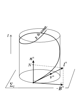
Fig. 1: Spacetime foliation $\mathchar 28934\relax_{t}$, helicoidal Killing vector $l$ and its trajectories $x^{i^{\prime}}={\rm const}$, which are the worldlines of the co-orbiting observer (4-velocity: $v$). Also shown are the rotating-coordinate shift vector $B$ and the unit future-directed vector $n$, normal to the spacelike hypersurface $\mathchar 28934\relax_{t}$.

The approximation suggested above amounts to neglect outgoing gravitational radiation. For non-axisymmetric systems — as binaries are — imposing $l$ as an exact Killing vector leads to a spacetime which is not asymptotically flat [20]. Thus, in solving for the gravitational field equations, a certain approximation has to be devised in order to avoid the divergence of some metric coefficients at infinity. For instance such an approximation could be the Wilson & Mathews scheme [21] that amounts to solve only for the Hamiltonian and momentum constraint equations (cf. Sect. 3). This approximation has been used in all the relativistic studies to date and is consistent with the existence of the helicoidal Killing vector field (2.1). Note also that since the gravitational radiation reaction shows up only at the 2.5-PN order, the helicoidal symmetry is exact up to the 2-PN order.

Following the standard 3+1 formalism, we introduce a spacetime foliation by a family of spacelike hypersurfaces $\mathchar 28934\relax_{t}$ such that at spatial infinity, the vector $k$ introduced in Eq. (2.1) is normal to $\mathchar 28934\relax_{t}$ and the ADM 3-momentum in $\mathchar 28934\relax_{t}$ vanishes (i.e. the time $t$ is the proper time of an asymptotic inertial observer at rest with respect to the binary system). Asymptotically, $\mbox{\boldmath$k$}=\partial/\partial t$ and $\mbox{\boldmath$m$}=\partial/\partial\varphi$, where $\varphi$ is the azimuthal coordinate associated with the above asymptotic inertial observer, so that Eq. (2.1) can be re-written as

$$\mbox{\boldmath$l$}={\partial\over\partial t}+\mathchar 28938\relax\,{\partial\over\partial\varphi}\ .$$ (2.2)

One can then introduce the shift vector $B$ of co-orbiting coordinates by means of the orthogonal decomposition of $l$ with respect to the $\mathchar 28934\relax_{t}$ foliation (cf. Fig. 1):

$$\mbox{\boldmath$l$}=N\,\mbox{\boldmath$n$}-\mbox{\boldmath$B$},$$ (2.3)

$n$ being the unit future directed vector normal to $\mathchar 28934\relax_{t}$ and $N$ the lapse function.

2.2 Irrotational flow

We consider a perfect fluid, which constitutes an excellent approximation for neutron star matter. The matter stress energy tensor is then

$$\mbox{\boldmath$T$}=(e+p)\mbox{\boldmath$u$}\otimes\mbox{\boldmath$u$}+p\mbox{\boldmath$g$}\ ,$$ (2.4)

$e$ being the fluid proper energy density, $p$ the fluid pressure and $u$ the fluid 4-velocity. A zero-temperature equation of state (EOS) is a very good approximation for neutron star matter. For such an EOS, the first law of thermodynamics gives rise to the following identity (Gibbs-Duhem relation):

$${\nabla p\over e+p}={1\over h}\nabla h\ ,$$ (2.5)

where $h$ is the fluid specific enthalpy:

$$h:={e+p\over m_{\rm B}n},$$ (2.6)

$n$ being the fluid baryon number density and $m_{\rm B}$ the mean baryon mass: $m_{\rm B}=1.66\times 10^{-27}{\rm\ kg}$. Note that for our zero-temperature EOS, $m_{\rm B}\,h$ is equal to the fluid chemical potential.

By means of the identity (2.5), it is straightforward to show that the classical momentum-energy conservation equation $\nabla\cdot\mbox{\boldmath$T$}=0$ is equivalent to the set of two equations[22, 23]:

$$\mbox{\boldmath$u$}\cdot(\nabla\wedge\mbox{\boldmath$w$})=0\ ,$$ (2.7)

$$\nabla\cdot(n\mbox{\boldmath$u$})=0\ .$$ (2.8)

In Eq. (2.7), $w$ is the co-momentum 1-form

$$\mbox{\boldmath$w$}:=h\,\mbox{\boldmath$u$}$$ (2.9)

and $\nabla\wedge\mbox{\boldmath$w$}$ denotes the exterior derivative of $w$, i.e. the vorticity 2-form[22]. In terms of components, one has

$$(\nabla\wedge\mbox{\boldmath$w$})_{\alpha\beta}=\nabla_{\alpha}w_{\beta}-\nabla_{\beta}w_{\alpha}\ .$$ (2.10)

The advantage of writing the equation of motion in the form (2.7) rather than in the traditional form $\nabla\cdot\mbox{\boldmath$T$}=0$ is that one can see immediately that a flow of the form

$$\mbox{\boldmath$w$}=\nabla\mathchar 28937\relax\ ,$$ (2.11)

where $\mathchar 28937\relax$ is some scalar, is a solution of the equation of motion. Such a flow is called a potential flow. Indeed, Eq. (2.11) implies the vanishing of the vorticity 2-form:

$$\nabla\wedge\mbox{\boldmath$w$}=0\ ,$$ (2.12)

so that the equation of motion (2.7) is trivially satisfied. Equation (2.12) is the relativistic definition of an irrotational flow [22].

2.3 First integral of motion

The above two assumptions, namely (i) $l$ is a symmetry generator and (ii) the flow is irrotational, yield to the following first integral

$$h\,\mbox{\boldmath$l$}\cdot\mbox{\boldmath$u$}={\rm const}.$$ (2.13)

This was first pointed out by Carter [23]. The demonstration is straightforward if one applies the classical Cartan’s identity to the 1-form $w$ and the vector field $l$:

$$\pounds_{\mbox{\boldmath$l$}}\mbox{\boldmath$w$}=\mbox{\boldmath$l$}\cdot(\nabla\wedge\mbox{\boldmath$w$})+\nabla(\mbox{\boldmath$l$}\cdot\mbox{\boldmath$w$})\ ,$$ (2.14)

where $\pounds_{\mbox{\boldmath$l$}}$ denotes the Lie derivative along the vector field $l$. Hypothesis (i) implies that $\pounds_{\mbox{\boldmath$l$}}\mbox{\boldmath$w$}=0$ and hypothesis (ii) that $\nabla\wedge\mbox{\boldmath$w$}=0$, so that Eq. (2.14) reduces to

$$\nabla(\mbox{\boldmath$l$}\cdot\mbox{\boldmath$w$})=0\ ,$$ (2.15)

from which the first integral (2.13) follows.

2.4 Remark about Bernoulli’s theorem

Let us mention a point which seems to have been missed by various authors: the existence of the first integral of motion (2.13) is not merely the relativistic generalization of Bernoulli’s theorem. This latter follows solely from the existence of the symmetry generator $l$ and can be established as follows. Inserting $\pounds_{\mbox{\boldmath$l$}}\mbox{\boldmath$w$}=0$ into Cartan’s identity (2.14) yields

$$\mbox{\boldmath$l$}\cdot(\nabla\wedge\mbox{\boldmath$w$})+\nabla(\mbox{\boldmath$l$}\cdot\mbox{\boldmath$w$})=0\ .$$ (2.16)

Performing the scalar product by $u$ leads to

$$\mbox{\boldmath$l$}\cdot(\nabla\wedge\mbox{\boldmath$w$})\cdot\mbox{\boldmath$u$}+\mbox{\boldmath$u$}\cdot\nabla(\mbox{\boldmath$l$}\cdot\mbox{\boldmath$w$})=0\ .$$ (2.17)

The first term in the left-hand side vanishes by virtue of the equation of motion (2.7), so that one is left with

$$\mbox{\boldmath$u$}\cdot\nabla(\mbox{\boldmath$l$}\cdot\mbox{\boldmath$w$})=0\ ,$$ (2.18)

which means that the quantity $\mbox{\boldmath$l$}\cdot\mbox{\boldmath$w$}=h\,\mbox{\boldmath$l$}\cdot\mbox{\boldmath$u$}$ is constant along each streamline. This is the Bernoulli theorem. The key point is that, in order for the constant to be uniform over the streamlines (i.e. to be a constant over spacetime), as in Eq. (2.13), some additional property of the flow must be required. One well known possibility is rigidity (i.e. $u$ colinear to $l$) [24], which would apply to synchronized binaries. The alternative property with which we are concerned here is irrotationality.

2.5 Equation for the velocity potential $\mathchar 28937\relax$

Since Eq. (2.7) is trivially satisfied by the potential flow (2.11), the only part of the momentum-energy equation $\nabla\cdot\mbox{\boldmath$T$}=0$ which remains to be satisfied is Eq. (2.8) (baryon number conservation). Inserting Eq. (2.11) in Eq. (2.8) results in an equation for the velocity potential $\mathchar 28937\relax$:

$${n\over h}\nabla\cdot\nabla\mathchar 28937\relax+\nabla\mathchar 28937\relax\cdot\nabla\left({n\over h}\right)=0\ .$$ (2.19)

Following the 3+1 formalism, we introduce the 3-metric $h$ induced by $g$ into the $\mathchar 28934\relax_{t}$ hypersurfaces, and denote by $D$ the associated covariant derivative. Taking into account the helicoidal symmetry, Eq. (2.19) becomes

$$nD_{i}D^{i}\mathchar 28937\relax+D^{i}n\,D_{i}\mathchar 28937\relax=-{h\mathchar 28928\relax_{\rm n}\over N}B^{i}D_{i}n+n\left(D^{i}\mathchar 28937\relax\,D_{i}\ln{h\over N}-{B^{i}\over N}D_{i}\mathchar 28928\relax_{\rm n}\right)+Knh\mathchar 28928\relax_{\rm n}\ ,$$ (2.20)

where K is the trace of the extrinsic curvature tensor of the $\mathchar 28934\relax_{t}$ hypersurfaces and $\mathchar 28928\relax_{\rm n}$ is the Lorentz factor between the fluid observer and the Eulerian observer (observer whose 4-velocity is the unit normal $n$ to $\mathchar 28934\relax_{t}$):

$$\mathchar 28928\relax_{\rm n}:=-\mbox{\boldmath$n$}\cdot\mbox{\boldmath$u$}=\left(1+{1\over h^{2}}D_{i}\mathchar 28937\relax\,D^{i}\mathchar 28937\relax\right)^{1/2}\ .$$ (2.21)

3 A simplifying assumption: the conformally flat 3-metric

3.1 Presentation and justifications

The problem of finding irrotational binary configurations in quasiequilibrium amounts to solve the elliptic equation (2.20) for $\mathchar 28937\relax$ and the Einstein equations for the components of the metric tensor. As a first step, a simplifying assumption can be introduced, in order to reduce the computational task, namely to take the 3-metric induced in the hypersurfaces $\mathchar 28934\relax_{t}$ to be conformally flat:

$$\mbox{\boldmath$h$}=A^{2}\,\mbox{\boldmath$f$}\ ,$$ (3.1)

where $A$ is some scalar field and $f$ is a flat 3-metric. Note that this assumption, first introduced by Wilson & Mathews [21], is physically less justified than the assumptions of quasiequilibrium and irrotational flow discussed above. However, some possible justifications of (3.1) are

1. it is exact for spherically symmetric configurations;

2. it is very accurate for axisymmetric rotating neutron stars [25];

3. the 1-PN metric fits it;

4. the 2.5-PN metric deviates from it by only 2 % for two $1.4\,M_{\odot}$ neutron stars as close as 30 km (in harmonic coordinates) [26].

3.2 Partial differential equations for the metric

Assuming (3.1), the full spacetime metric takes the form

$$ds^{2}=-(N^{2}-B_{i}B^{i})dt^{2}-2B_{i}dt\,dx^{i}+A^{2}f_{ij}dx^{i}\,dx^{j}\ .$$ (3.2)

We have thus five metric functions to determine: the lapse $N$, the conformal factor $A$ and the three components $B^{i}$ of the shift vector. Let us introduce auxiliary metric quantities: the shift vector of non-rotating coordinates:

$$\mbox{\boldmath$N$}=\mbox{\boldmath$B$}+\mathchar 28938\relax{\partial\over\partial\varphi}\ ,$$ (3.3)

and the two logarithms

$$\beta:=\ln(AN),$$ (3.4)

$$\nu:=\ln N\ .$$ (3.5)

At the Newtonian limit $\beta=0$ and $\nu$ coincides with the Newtonian gravitational potential.

In the following, we choose maximal slicing coordinates, for which $K=0$.

The Killing equation $\nabla_{\alpha}l_{\beta}+\nabla_{\beta}l_{\alpha}=0$ give rise to a relation between the $\mathchar 28934\relax_{t}$ extrinsic curvature tensor $K$ and the shift vector $N$:

$$K^{ij}=-{1\over 2A^{2}N}\left\{{\overline{\nabla}}^{i}N^{j}+{\overline{\nabla}}^{j}N^{i}-{2\over 3}f^{ij}{\overline{\nabla}}_{k}N^{k}\right\}\ ,$$ (3.6)

where ${\overline{\nabla}}$ stands for the covariant derivative associated with the flat 3-metric $f$.

The trace of the spatial part of the Einstein equation, combined with the Hamiltonian constraint equation, result in the following two equations

$$\underline{\mathchar 28929\relax}\beta=4\pi A^{2}S+{3\over 4}A^{2}K_{ij}K^{ij}-{1\over 2}\left({\overline{\nabla}}_{i}\nu{\overline{\nabla}}^{i}\nu+{\overline{\nabla}}_{i}\beta{\overline{\nabla}}^{i}\beta\right)\ ,$$ (3.7)

$$\underline{\mathchar 28929\relax}\nu=4\pi A^{2}(E+S)+A^{2}K_{ij}K^{ij}-{\overline{\nabla}}_{i}\nu{\overline{\nabla}}^{i}\beta\ ,$$ (3.8)

where $\underline{\mathchar 28929\relax}:={\overline{\nabla}}^{i}{\overline{\nabla}}_{i}$ is the Laplacian operator associated with the flat metric $f$, $E$ and $S$ are respectively the matter energy density and trace of the stress tensor, both as measured by the Eulerian observer:

$$E:=\mbox{\boldmath$n$}\cdot\mbox{\boldmath$T$}\cdot\mbox{\boldmath$n$}=\mathchar 28928\relax_{\rm n}^{2}(e+p)-p,$$ (3.9)

$$S:=\mbox{\boldmath$h$}\cdot\mbox{\boldmath$T$}=3p+(E+p)U_{i}U^{i}\ ,$$ (3.10)

$U^{i}$ being the fluid 3-velocity as measured by the Eulerian observer:

$$\mbox{\boldmath$U$}:={1\over\mathchar 28928\relax_{\rm n}}\,\mbox{\boldmath$h$}\cdot\mbox{\boldmath$u$}\ .$$ (3.11)

For the potential flow (2.11), $U^{i}$ is related to $\mathchar 28937\relax$ by

$$U^{i}={1\over A^{2}\mathchar 28928\relax_{\rm n}h}{\overline{\nabla}}^{i}\mathchar 28937\relax\ .$$ (3.12)

By the means of Eq. (3.6), the momentum constraint equation yields

$$\underline{\mathchar 28929\relax}N^{i}+{1\over 3}{\overline{\nabla}}^{i}\left({\overline{\nabla}}_{j}N^{j}\right)=-16\pi NA^{2}(E+p)U^{i}+2NA^{2}K^{ij}{\overline{\nabla}}_{j}(3\beta-4\nu)\ .$$ (3.13)

The equations to be solved to get the metric coefficients are the elliptic equations (3.7), (3.8) and (3.13). Note that they represent only five of the ten Einstein equations. The remaining five Einstein equations are not used in this procedure. Moreover, some of these remaining equations are certainly violated, reflecting the fact that the conformally flat 3-metric (3.1) is an approximation to the exact metric generated by a binary system.

At the Newtonian limit, Eqs. (3.7) and (3.13) reduce to $0=0$. There remains only Eq. (3.8), which gives the usual Poisson equation for the gravitational potential $\nu$.

3.3 Equation for the matter

Taking the logarithm of the first integral of motion (2.13) and using the metric (3.2) yields

$$H+\nu+\ln\mathchar 28928\relax_{\rm n}+\ln\left(1+A^{2}f_{ij}{B^{i}\over N}U^{j}\right)={\rm const}\ ,$$ (3.14)

where $H$ is the logarithm of the specific enthalpy:

$$H:=\ln h\ .$$ (3.15)

At the Newtonian limit, $H$ coincides with the specific non-relativistic (i.e. which does not include the rest mass energy) enthalpy.

Taking into account Eqs. (2.21) and (3.3), the Newtonian limit of the first integral (3.14) is

$$H+\nu+{1\over 2}(\nabla\mathchar 28937\relax)^{2}-(\mbox{\boldmath$\mathchar 28938\relax$}\times\mbox{\boldmath$r$})\cdot\nabla\mathchar 28937\relax={\rm const}.$$ (3.16)

(Recall that $\nu$ reduces to the Newtonian gravitational potential). We recognize the classical expression [compare e.g. with Eq. (12) of Ref. ? or Eq. (11) of Ref. ?].

For a zero-temperature EOS, $H$ can be considered as a function of the baryon density $n$ solely, so that one can introduce the thermodynamical coefficient

$$\zeta:={d\ln H\over d\ln n}\ .$$ (3.17)

The gradient of $n$ which appears in Eq. (2.20) can be then replaced by a gradient of $H$ so that, using the metric (3.1), one obtains

$$\zeta H\underline{\mathchar 28929\relax}\mathchar 28937\relax+{\overline{\nabla}}^{i}H{\overline{\nabla}}_{i}\mathchar 28937\relax=-A^{2}h\mathchar 28928\relax_{\rm n}{B^{i}\over N}{\overline{\nabla}}_{i}H+\zeta H\left({\overline{\nabla}}^{i}\mathchar 28937\relax{\overline{\nabla}}_{i}(H-\beta)-A^{2}{B^{i}\over N}h{\overline{\nabla}}_{i}\mathchar 28928\relax_{\rm n}\right)\ .$$ (3.18)

Note that this is not a Poisson-type equation for $\mathchar 28937\relax$, because the coefficient $H$ in front of the Laplacian operator vanishes at the surface of the star. Numerically speaking, this means that this equation must be dealt by a specific technique and not by the direct use of some Poisson solver.

At the Newtonian limit Eq. (3.18) reduces to

$$\zeta H\mathchar 28929\relax\mathchar 28937\relax+\nabla H\cdot\nabla\mathchar 28937\relax=(\mbox{\boldmath$\mathchar 28938\relax$}\times\mbox{\boldmath$r$})\cdot\nabla H\ .$$ (3.19)

Here again, we recognize the classical expression [compare e.g. with Eq. (13) of Ref. ?].

4 Analytical approach

The above equations cannot be solved analytically, unless additional simplifying assumptions are introduced. Two such assumptions are that

1. the fluid is incompressible;

2. the 1-PN approximation to general relativity is used.

These assumptions have recently allowed Taniguchi[28] to find analytical solutions to the relativistic irrotational Darwin-Riemann problem. Note that at the 1-PN level, the figures are no longer ellipsoids, even for an incompressible fluid. This is explicitely taken into account in Taniguchi’s procedure [28], which improves over a previous 1-PN study by Lombardi, Rasio & Shapiro [29], where the figures where assumed to be ellipsoidal.

The main findings of Taniguchi’s study[28] are that the orbital separation at the innermost stable circular orbit (ISCO) is lower than in the Newtonian case, whereas the orbital angular at the ISCO is roughly the same than in the Newtonian case.

5 Numerical approaches

Recently three groups have obtained numerical solutions of the partial differential equations presented in Sect. 3, by the mean of different numerical techniques. In chronological order, these groups are

• our group [30, 26], which has employed a multi-domain spectral method [31] with spherical coordinates;

• Marronetti, Mathews & Wilson [32, 33], who have employed single-domain finite differences with Cartesian coordinates;

• Uryu & Eriguchi [34], who have employed multi-domain finite differences with spherical coordinates.

In this Section, we discuss only the numerical technique developed in our group, whereas in Sect. 6, we will present the results obtained by the three groups.

Fig. 2: Logarithm of the relative global error of the numerical solution with respect to the number of degrees of freedom in $\theta$ for a Roche ellipsoid for an equal mass binary system and $\mathchar 28938\relax^{2}/(\pi G\rho)=0.1147$ (the numbers of degrees of freedom in the other directions are $N_{r}=2N_{\theta}-1$ and $N_{\varphi}=N_{\theta}-1$)[31]. Also shown is the error in the verification of the virial theorem.

5.1 Brief description of the multi-domain spectral method

The numerical procedure to solve the PDE system presented in Sect. 3 is based on the multi-domain spectral method developed in Ref. ?. We simply recall here some basic features of the method:

• Spherical-type coordinates $(\xi,\theta^{\prime},\varphi^{\prime})$ centered on each star are used: this ensures a much better description of the stars than by means of Cartesian coordinates.

• These spherical-type coordinates are surface-fitted coordinates: i.e. the surface of each star lies at a constant value of the coordinate $\xi$ thanks to a mapping $(\xi,\theta^{\prime},\varphi^{\prime})\mapsto(r,\theta,\varphi)$ [see Ref. ? for details about this mapping]. This ensures that the spectral method applied in each domain is free from any Gibbs phenomenon (spurious oscillations generated by discontinuities).

• The outermost domain extends up to spatial infinity, thanks to the mapping $1/r=(1-\xi)/(2R_{0})$. This enables us to put exact boundary conditions on the elliptic equations (3.7), (3.8) and (3.13) for the metric coefficients: spatial infinity is the only location where the metric is known in advance (Minkowski metric).

• Thanks to the use of a spectral method [35] in each domain, the numerical error is evanescent, i.e. it decreases exponentially with the number of coefficients (or equivalently grid points) used in the spectral expansions, as shown in Fig. 2.

The PDE system to be solved being non-linear, we use an iterative procedure. The iteration is stopped when the relative difference in the enthalpy field between two successive steps goes below a certain threshold, typically $10^{-7}$. An illustrative solution is shown in Fig. 3.

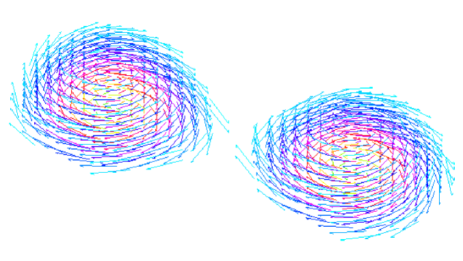
Fig. 3: Velocity field with respect to the co-orbiting frame in a irrotational binary system (only the part of the stars above the orbital plane is represented).

The numerical code is written in the LORENE language [36], which is a C++ based language for numerical relativity. A typical run make use of $N_{r}=33$, $N_{\theta}=21$, and $N_{\varphi}=20$ coefficients (= number of collocation points, which may be seen as number of grid points) in each of the domains. 8 domains are used : 3 for each star and 2 domains centered on the intersection between the rotation axis and the orbital plane. The corresponding memory requirement is 155 MB. A computation involves $\sim 250$ steps, which takes 9 h 30 min on one CPU of a SGI Origin200 computer (MIPS R10000 processor at 180 MHz). Note that due to the rather small memory requirement, runs can be performed in parallel on a multi-processor platform. This especially useful to compute sequences of configurations.

5.2 Tests passed by the code

In the Newtonian and incompressible limit, the analytical solution constituted by a Roche ellipsoid is recovered with a relative accuracy of $\sim 10^{-9}$, as shown in Fig. 2. For compressible and irrotational Newtonian binaries, no analytical solution is available, but the virial theorem can be used to get an estimation of the numerical error: we found that the virial theorem is satisfied with a relative accuracy of $10^{-7}$. Preliminary comparisons with the irrotational Newtonian configurations recently computed by Uryu & Eriguchi [37, 27] reveal a good agreement. Regarding the relativistic case, we have checked our procedure of resolution of the gravitational field equations by comparison with the results of Baumgarte et al. [38] which deal with corotating binaries [our code can compute corotating configurations by setting to zero the velocity field of the fluid with respect to the co-orbiting observer]. We have performed the comparison with the configuration $z_{A}=0.20$ in Table V of Ref. ?. We used the same equation of state (EOS) (polytrope with $\gamma=2$), same value of the separation $r_{C}$ and same value of the maximum density parameter $q^{\rm max}$. We found a relative discrepancy of $1.1\%$ on $\mathchar 28938\relax$, $1.4\%$ on $M_{0}$, $1.1\%$ on $M$, $2.3\%$ on $J$, $0.8\%$ on $z_{A}$, $0.4\%$ on $r_{A}$ and $0.07\%$ on $r_{B}$ (using the notations of Ref. ?).

6 Numerical results

6.1 Equation of state and compactification ratio

As a simplified model for nuclear matter, let us consider a polytropic EOS with an adiabatic index $\gamma=2$:

$$p=\kappa(m_{\rm B}n)^{\gamma}\ ,\qquad e=m_{\rm B}n+p/(\gamma-1)\ ,$$ (6.1)

with $\kappa=1.8\times 10^{-2}{\ \rm J\,m}^{3}{\rm kg}^{-2}$. This EOS is the same as that used by Mathews, Marronetti and Wilson (Sect. IV A of Ref ?).

Fig. 4: Mass as a function of the central energy density for static isolated neutron stars constructed with the EOS (6.1). The heavy dots are configurations considered by our group [30, 26], Marronetti et al. [39, 32, 33], and Uryu & Eriguchi [34] (see text) ($\rho_{\rm nuc}:=1.66\times 10^{17}{\rm\ kg\,m}^{-3}$).

The mass – central density curve of static configurations in isolation constructed upon this EOS is represented in Fig. 4. The three points on this curve corresponds to three configurations studied by the various groups mentioned in the beginning of Sect. 5:

• The configuration of baryon mass $M_{\rm B}=1.625\,M_{\odot}$ and compactification ratio $M/R=0.14$ is that considered in the dynamical study of Mathews, Marronetti and Wilson [39] and in the quasiequilibrium studies of our group [30, 26], of Marronetti et al. [33], and of Uryu & Eriguchi [34].

• The configuration of baryon mass $M_{\rm B}=1.85\,M_{\odot}$ and compactification ratio $M/R=0.17$ has been studied by our group [26] and Uryu & Eriguchi [34].

• The configuration of baryon mass $M_{\rm B}=1.95\,M_{\odot}$ and compactification ratio $M/R=0.19$ has been studied by Marronetti et al.[32, 33] .

6.2 Irrotational sequence with $M/R=0.14$

In this section, we give some details about the irrotational sequence $M_{\rm B}=1.625\,M_{\odot}$ presented in Ref. ?. This sequence starts at the coordinate separation $d=110{\rm\ km}$ (orbital frequency $f=82{\rm\ Hz}$), where the two stars are almost spherical, and ends at $d=41{\rm\ km}$ ($f=332{\rm\ Hz}$), where a cusp appears on the surface of the stars, which means that the stars start to break. The shape of the surface at this last point is shown in Fig. 5.

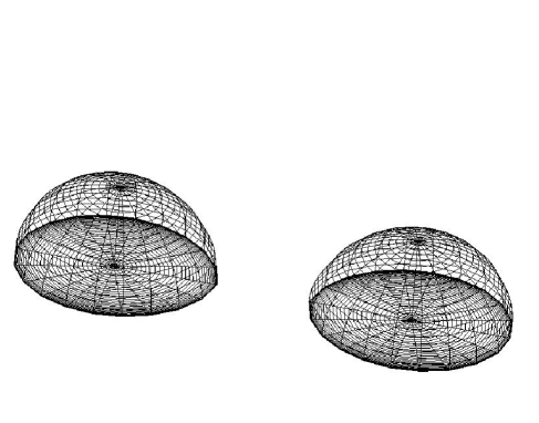
Fig. 5: Shape of irrotational binary neutron stars of baryon mass $M_{\rm B}=1.625\,M_{\odot}$, when the coordinate separation between their centers (density maxima) is $41{\rm\ km}$. Only one half of each star is represented (the part which is above the orbital plane). The drawing is that of the numerical grid, which coincides with the surface of the star, thanks to the use of surface-fitted spherical coordinates.

The velocity field with respect to the co-orbiting observer, as defined by Eq. (52) of Ref. ?, is shown in Fig. 6. Note that this field is tangent to the surface of the star, as it must be.

The lapse function $N$ is represented in Fig. 7. The coordinate system $(x,y,z)$ is centered on the intersection between the rotation axis and the orbital plane. The $x$ axis joins the two stellar centers, and $z=0$ is the orbital plane. The value of $N$ at the center of each star is $N_{\rm c}=0.64$, whereas the central value of the conformal factor $A^{2}$ is $A^{2}_{\rm c}=2.20$. The shift vector of non-rotating coordinates, $\bf N$, is shown in Fig. 8. Its maximum value is $0.10\,c$.

Fig. 6: Velocity field with respect to the co-orbiting observer, for the configuration shown in Fig. 5. The plane of the figure is the orbital plane. The heavy line denotes the surface of the star. The companion is located at $x=+41{\rm\ km}$.

Fig. 7: Isocontour of the lapse function $N$ for the configuration shown in Fig. 5. The plots are cross section in the $x=0$, $y=0$ and $z=0$ planes (note that the $x$ coordinate is shifted by $20.5{\rm\ km}$ with respect to that of Fig. 6). The dot-dashed line denotes the boundary between the inner numerical grid and the outer compactified one (which extends to spatial infinity), for the grid system centered on the intersection between the rotation axis and the orbital plane.

Fig. 8: Shift vector of non-rotating coordinates in the orbital plane, for the configuration shown in Figs. 5-7.

The variation of the central density along the $M_{\rm B}=1.625\,M_{\odot}$ sequence is shown in Fig. 9. We have also computed a corotating (i.e. synchronized) sequence for comparison (dashed line in Fig. 9). In the corotating case, the central density decreases quite substantially as the two stars approach each other. This is in agreement with the results of Baumgarte et al. [40, 38]. In the irrotational case (solid line in Fig. 9), the central density remains rather constant (with a slight increase, below $0.1\%$) before decreasing. This contrasts with the result of the dynamical calculations by Mathews et al. [39] which showed a central density increase of $14\%$ for the same compactification ratio $M/R=0.14$. But, as stated in Sect. 1, this last result has revealed to be spurious due to some error in a formula employed in the code [6].

It is worth to note that, for the same compactification ratio $M/R=0.14$, the computations by the other groups show a central density variation in accordance with the one presented above: it is at most 1% both in the results of Marronetti et al. [33] and Uryu & Eriguchi [34].

We can thus conclude that no tendency to individual gravitational collapse is found when the orbit shrinks.

Fig. 9: Relative variation of the central energy density $e_{\rm c}$ with respect to its value at infinite separation $e_{\rm c}^{\rm inf}$ as a function of the coordinate separation $d$ (or of the orbital frequency $\mathchar 28938\relax/(2\pi)$) for constant baryon mass $M_{\rm B}=1.625\,M_{\odot}$ sequences[30]. The solid (resp. dashed) line corresponds to a irrotational (resp. corotating) sequence of coalescing neutron star binaries.

6.3 Irrotational sequence with $M/R=0.17$

In order to investigate the dependency of the above result on the compactness of the stars, we have computed an irrotational sequence with a baryon mass $M_{\rm B}=1.85\,M_{\odot}$, which corresponds to a compactification ratio $M/R=0.17$ for stars at infinite separation (second heavy dot in Fig. 4) [26]. The result is compared with that of $M/R=0.14$ in Fig. 10. A very small density increase (at most $0.3\%$) is observed before the decrease. For the same compactification ratio $M/R=0.17$, Uryu & Eriguchi [34] report a slightly higher increase (1.5 %).

This density increase remains within the expected error ($\sim 2\%$, cf. Sect. 3.1) induced by the conformally flat approximation for the 3-metric, so that it cannot be asserted that this effect would remain in a complete calculation.

6.4 Irrotational sequence with $M/R=0.19$

Marronetti, Mathews and Wilson [32, 33] have computed quasiequilibrium irrotational configurations with a compactification ratio $M/R=0.19$ (third heavy dot in Fig. 4). They found a central density increase, as the orbit shrinks, of the order of $1.5\%$. This still remains within the error introduced by the conformally flat approximation.

Fig. 10: Relative variation of the central energy density $e_{\rm c}$ with respect to its value at infinite separation $e_{\rm c}^{\rm inf}$ as a function of the coordinate separation $d$ for constant baryon mass sequences with $M_{\rm B}=1.625\,M_{\odot}$ (solid line, same as in Fig. 9) and $M_{\rm B}=1.85\,M_{\odot}$ (dashed line).

7 Innermost stable circular orbit

An important parameter for the detection of a gravitational wave signal from coalescing binaries is the location of the innermost stable circular orbit (ISCO), if any. In Table I, we recall what is known about the existence of an ISCO for extended fluid bodies. The case of two point masses is discussed in details in Ref. [41].

Model	Existence of an ISCO	References
Newtonian corotating	ISCO $\Leftrightarrow\,\gamma>2$	?
Newtonian irrotational	ISCO $\Leftrightarrow\,\gamma>2.4$	?
GR corotating	ISCO $\Leftrightarrow\,\gamma>5/3$	?, ?
GR irrotational	ISCO exists for $\gamma=\infty$	?

Table I: Known results about the existence of an ISCO for extended fluid bodies, in terms of the adiabatic index $\gamma$.

For Newtonian binaries, it has been shown [43] that the ISCO is located at a minimum of the total energy, as well as total angular momentum, along a sequence at constant baryon number and constant circulation (irrotational sequences are such sequences). The instability found in this way is dynamical. For corotating sequences, it is secular instead [43, 2]. This turning point method also holds for locating ISCO in relativistic corotating binaries [44]. For relativistic irrotational configurations, no rigorous theorem has been proven yet about the localization of the ISCO by a turning point method. All what can be said is that no turning point is present in the irrotational sequences considered in Sect. 6: Fig. 11 shows the variation as the orbit shrinks of the ADM mass of the spatial hypersurface $t={\rm const}$ (which is a measure of the total energy, or equivalently of the binding energy, of the system), as well as of the total angular momentum, for the evolutionary sequences with $M/R=0.14$ and $M/R=0.17$. Clearly, both the ADM mass and the angular momentum decreases monoticaly, without showing any turning point. The same result has been found by Marronetti et al. [Fig. 2 of Ref. ?, which also shows the good agreement between Marronetti et al.[33] results and ours[26]] and Uryu & Eriguchi [Fig. 5 of Ref. ?].

Fig. 11: Variation of (half of) the ADM mass (left) and of the total angular momentum (right) of the binary system with respect to the coordinate distance $d$, along the evolutionary sequences $M_{\rm B}=1.625\,M_{\odot}$, $M/R=0.14$ (top) and $M_{\rm B}=1.85\,M_{\odot}$, $M/R=0.17$ (bottom) [from Ref. [26]]

.

References

- [1] S. Chandrasekhar, Ellipsoidal figures of equilibrium (Yale University Press, New Haven, 1969).
- [2] D. Lai, F.A. Rasio, and S.L. Shapiro, Astrophys. J. 420 (1994), 811.
- [3] Y. Eriguchi, this volume.
- [4] J.R. Wilson and G.J. Mathews, Phys. Rev. Lett. 75 (1995), 4161.
- [5] J.R. Wilson, G.J. Mathews, and P. Marronetti, Phys. Rev. D 54 ( 1996), 1317.
- [6] E.E. Flanagan, Phys. Rev. Lett. 82 (1999), 1354.
- [7] C.S. Kochanek, Astrophys. J. 398 (1992), 234.
- [8] L. Bildsten and C. Cutler, Astrophys. J. 400 (1992), 175.
- [9] W.M. Suen, this volume.
- [10] K. Oohara, this volume.
- [11] M. Shibata, Phys. Rev. D, in press (preprint: gr-qc/9908027).
- [12] S Bonazzola, E. Gourgoulhon, P. Haensel, and J-A. Marck, in Approaches to Numerical Relativity, ed. R.A. d’Inverno (Cambridge University Press, Cambridge, England, 1992), p. 230.
- [13] S. Bonazzola, E. Gourgoulhon, and J-A. Marck, Phys. Rev. D 56 (1997), 7740.
- [14] H. Asada, Phys. Rev. D 57 (1998), 7292.
- [15] S.A. Teukolsky, Astrophys. J. 504 (1998), 442.
- [16] M. Shibata, Phys. Rev. D 58 (1998), 024012.
- [17] L.D. Landau and E.M. Lifchitz, Mécanique des fluides (Mir, Moscow, 1989).
- [18] L. Blanchet, T. Damour, B.R. Iyer, C.M. Will, A.G. Wiseman, Phys. Rev. Lett. 74 (1995), 3515.
- [19] P.C. Peters, Phys. Rev. 136 (1964), B1224.
- [20] G.W. Gibbons, J.M. Stewart, in Classical General Relativity, eds. W.B. Bonnor, J.N. Islam and M.A.H. MacCallum (Cambridge University Press, Cambridge, England, 1983), p. 77.
- [21] J.R. Wilson, G.J Mathews, in Frontiers in Numerical Relativity, eds. C.R. Evans, L.S. Finn and D.W. Hobill, (Cambridge University Press, Cambridge, England, 1989).
- [22] A. Lichnerowicz, Relativistic hydrodynamics and magnetohydrodynamics (Benjamin, New York, 1967).
- [23] B. Carter, in Active Galactic Nuclei, eds. C. Hazard and S. Mitton (Cambridge University Press, Cambridge, England, 1979), p. 273.
- [24] R.H. Boyer, Proc. Cambridge Phil. Soc. 61 (1965), 527.
- [25] G.B. Cook, S.L. Shapiro, and S.A. Teukolsky, Phys. Rev. D 53 (1996), 5533.
- [26] S. Bonazzola, E. Gourgoulhon, and J-A. Marck, to appear in the Proceedings of the 19th Texas Symposium on Relativistic Astrophysics (CD-ROM version) (preprint: gr-qc/9904040).
- [27] K. Uryu and Y. Eriguchi, Astrophys. J. Suppl. 118 (1998), 563.
- [28] K. Taniguchi, Prog. Theor. Phys. 101 (1999), 283.
- [29] J.C. Lombardi, F.A. Rasio, S.L. Shapiro, Phys. Rev. D 56 (1997), 3416.
- [30] S. Bonazzola, E. Gourgoulhon, and J-A. Marck, Phys. Rev. Lett. 82 (1999), 892.
- [31] S. Bonazzola, E. Gourgoulhon, and J-A. Marck, Phys. Rev. D 58 (1998), 104020.
- [32] P. Marronetti, G.J. Mathews, and J.R. Wilson, to appear in the Proceedings of the 19th Texas Symposium on Relativistic Astrophysics (CD-ROM version) (preprint: gr-qc/9903105).
- [33] P. Marronetti, G.J. Mathews, and J.R. Wilson, Phys. Rev. D, in press (preprint: gr-qc/9906088).
- [34] K. Uryu, Y. Eriguchi, preprint gr-qc/9908059.
- [35] S. Bonazzola, E. Gourgoulhon, and J-A. Marck, J. Comp. Appl. Math., in press (preprint: gr-qc/9811089).
- [36] J-A. Marck, E. Gourgoulhon, and P. Grandclément, Langage Objet pour la RElativité NumériquE – library documentation, in preparation.
- [37] K. Uryu and Y. Eriguchi, Mon. Not. Roy. Astron. Soc. 296 (1998), L1.
- [38] T.W. Baumgarte, G.B. Cook, M.A. Scheel, S.L. Shapiro, and S.A. Teukolsky, Phys. Rev. D 57 (1998), 7299.
- [39] G.J. Mathews, P. Marronetti, and J.R. Wilson, Phys. Rev. D 58 (1998), 043003.
- [40] T.W. Baumgarte, G.B. Cook, M.A. Scheel, S.L. Shapiro, and S.A. Teukolsky, Phys. Rev. Lett. 79 (1997), 1182.
- [41] A. Buonanno, T. Damour, Phys. Rev. D 59 (1999), 084006.
- [42] M. Shibata, K. Taniguchi, T. Nakamura, Prog. Theor. Phys. Suppl. 128 (1997), 295.
- [43] D. Lai, F.A. Rasio, S.L. Shapiro, Astrophys. J. Suppl. 88 (1993), 205.
- [44] T.W. Baumgarte, G.B. Cook, M.A. Scheel, S.L. Shapiro, and S.A. Teukolsky, Phys. Rev. D 57 (1998), 6181.