IFUP-TH 20/99

May 1999

Gravitational Wave Experiments and

Early Universe Cosmology
Michele Maggiore
INFN, sezione di Pisa, and Dipartimento di Fisica, Università di Pisa
via Buonarroti 2, I-56127 Pisa, Italy

Gravitational-wave experiments with interferometers and with resonant masses can search for stochastic backgrounds of gravitational waves of cosmological origin. We review both experimental and theoretical aspects of the search for these backgrounds. We give a pedagogical derivation of the various relations that characterize the response of a detector to a stochastic background. We discuss the sensitivities of the large interferometers under constructions (LIGO, VIRGO, GEO600, TAMA300, AIGO) or planned (Avdanced LIGO, LISA) and of the presently operating resonant bars, and we give the sensitivities for various two-detectors correlations. We examine the existing limits on the energy density in gravitational waves from nucleosynthesis, COBE and pulsars, and their effects on theoretical predictions. We discuss general theoretical principles for order-of-magnitude estimates of cosmological production mechanisms, and then we turn to specific theoretical predictions from inflation, string cosmology, phase transitions, cosmic strings and other mechanisms. We finally compare with the stochastic backgrounds of astrophysical origin.

To appear in Physics Reports

1 Introduction

A large effort is presently under way in the scientific community for the construction of the first generation of large scale interferometers for gravitation wave (GW) detection. The two LIGO detectors are under construction in the US, and the Italian-French interferometer VIRGO is presently under construction near Pisa, Italy. The detectors are expected to start taking data around the year 2002, with a sensitivity where we might find signals from known astrophysical sources. These detectors are also expected to evolve into second generation experiments, with might better sensitivities. At the same time, two other somewhat smaller interferometers are being built: GEO600 in Germany and TAMA300 in Japan, and they will be important also for developing the techniques needed by second generation experiments. To cover the low-frequency region, where many interesting signals are expected, but which on the Earth is unaccessible because of seismic noise, it is planned to send an interferometer into space: this extraordinary experiment is LISA, which has been selected by the European Space Agency has a cornerstone mission in his future science program Horizons 2000 Plus, and might flight somewhere around 2010-2020, with a sensitivity levels where many sources are virtually guaranteed. Finally, although at a lower sensitivity level, cryogenic resonant bars are in operation since 1990, and more sensitive resonant masses, e.g. of spherical shape, are under study.

A possible target of these experiments is a stochastic background of GWs of cosmological origin. The detection of such a background would have a profound impact on early Universe cosmology and on high-energy physics, opening up a new window and exploring very early times in the evolution of the Universe, and correspondingly high energies, that will never be accessible by other means. The basic reason why relic GWs carry such a unique information is that particles which decoupled from the primordial plasma at time $t\sim t_{\rm dec}$, when the Universe had a temperature $T_{\rm dec}$, give a ‘snapshot’ of the state of the Universe at $T\sim T_{\rm dec}$. All informations on the Universe when the particle was still in thermal equilibrium has instead been obliterated by the successive interactions. The weaker the interaction of a particle, the higher is the energy scale when they drop out of thermal equilibrium. Hence, GWs can probe deeper into the very early Universe.

To be more quantitative, the condition for thermal equilibrium is that the rate $\Gamma$ of the processes that mantain equilibrium be larger than the rate of expansion of the Universe, as measured by the Hubble parameter $H$. The rate (in units $\hbar=c=1$) is given by $\Gamma=n\sigma|v|$ where $n$ is the number density of the particle in question, and for massless or light particles in equilibrium at a temperature $T$, $n\sim T^{3}$; $|v|\sim 1$ is the typical velocity and $\sigma$ is the cross-section of the process. Consider for instance the weakly interacting neutrinos. In this case the equilibrium is mantained, e.g., by electron-neutrino scattering, and at energies below the $W$ mass $\sigma\sim G_{F}^{2}\langle E^{2}\rangle\sim G_{F}^{2}T^{2}$ where $G_{F}$ is the Fermi constant and $\langle E^{2}\rangle$ is the average energy squared. The Hubble parameter during the radiation dominated era is related to the temperature by $H\sim T^{2}/M_{\rm Pl}$. Therefore

$$\left(\frac{\Gamma}{H}\right)_{\rm neutrino}\sim\frac{G_{F}^{2}T^{5}}{T^{2}/M_{\rm Pl}}\simeq\left(\frac{T}{1\rm MeV}\right)^{3}\,.$$ (1)

Even the weakly interacting neutrinos, therefore, cannot carry informations on the state of the Universe at temperatures larger than approximately 1 MeV. If we repeat the above computation for gravitons, the Fermi constant $G_{F}$ is replaced by Newton constant $G=1/M_{\rm Pl}^{2}$, where $M_{\rm Pl}\sim 10^{19}$ GeV is the Planck mass. At energies below $M_{\rm Pl}$,

$$\left(\frac{\Gamma}{H}\right)_{\rm graviton}\sim\left(\frac{T}{M_{\rm Pl}}\right)^{3}\,.$$ (2)

The gravitons are therefore decoupled below the Planck scale. It follows that relic gravitational waves are a potential source of informations on very high-energy physics. Gravitational waves produced in the very early Universe have not lost memory of the conditions in which they have been produced, as it happened to all other particles, but still retain in their spectrum, typical frequency and intensity, important informations on the state of the very early Universe, and therefore on physics at correspondingly high energies, which cannot be accessed experimentally in any other way. It is also clear that the property of gravitational waves that makes them so interesting, i.e. their extremely small cross section, is also responsible for the difficulties of the experimental detection.

In this review we will examine a number of experimental and theoretical aspects of the search for a stochastic background of GWs. The paper is organized as follows. We start from the experimental side; in sects. 2 to 4 we present the basic concepts for characterizing a stochastic background and for describing the detector. This seems to be a subject where everybody has its own definitions and notations, and we made an effort to clean up many formulas appearing in the literature, to present them in what we consider the clearest form, and to give the most straightforward derivation of various relations.

In sect. 5 we examine the various detectors under construction or already operating; we show the sensitivity curves of LIGO, VIRGO, GEO600, Advanced LIGO, LISA and NAUTILUS (kindly provided by the various collaborations), and we discuss the limiting sources of noise and the perspectives for improvement in the near and mid-term future.

To detect a stochastic background with Earth-based detectors, it turns out that it is mandatory to correlate two or more detectors. The sensitivities that can be reached with two-detectors correlations are discussed in sect. 6. We will show graphs for the overlap reduction functions between VIRGO and the other major detectors, and we will give the estimate of the minimum detectable value of the signal.

In sect. 7 we examine the existing bounds on the energy density in GWs coming from nucleosynthesis, COBE, msec pulsars, binary pulsar orbits, pulsar arrays.

Starting from sect. 8 we move toward more theoretical issues. First of all, we discuss general principles for order of magnitude estimate of the characteristic frequency and intensity of the stochastic background produced by cosmological mechanisms. With the very limited experimental informations that we have on the very high energy region, $M_{\rm GUT}\raise 1.72218pt\hbox{$<$}\kern-8.00003pt\lower 2.6694pt\hbox{$\sim$}E\raise 1.72218pt\hbox{$<$}\kern-8.00003pt\lower 2.6694pt\hbox{$\sim$}M_{\rm Pl}$, and on the history of the very early Universe, it is unlikely that theorists will be able to foresee all the interesting sources of relic stochastic backgrounds, let alone to compute their spectra. This is particularly clear in the Planckian or string theory domain where, even if we succeed in predicting some interesting physical effects, in general we cannot compute them reliably. So, despite the large efforts that have been devoted to understanding possible sources, it is still quite possible that, if a relic background of gravitational waves will be detected, its physical origin will be a surprise. In this case it is useful to understand what features of a theoretical computation have some general validity, and what are specific to a given model, separating for instance kinematical from dynamical effects. The results of this section provide a sort of benchmark, against which we can compare the results from the specific models discussed in sect. 9 and 10.

In sect. 9 we discuss the most general cosmological mechanism for GW production, namely the amplification of vacuum fluctuations. We examine both the case of standard inflation, and a more recent model, derived from string theory, known as pre-big-bang cosmology. In sect. 10 we examine a number of other production mechanisms.

Finally, in sect. 11 we discuss the stochastic background due to many unresolved astrophysical sources, which from the point of view of the cosmological background is a ‘noise’ that can compete with the signal (although, of course, it is very interesting in its own right).

2 Characterization of stochastic backgrounds of GWs

A stochastic background of GWs of cosmological origin is expected to be isotropic, stationary and unpolarized. Its main property will be therefore its frequency spectrum. There are different useful characterization of the spectrum: (1) in terms of a (normalized) energy density per unit logarithmic interval of frequency, $h_{0}^{2}\Omega_{\rm gw}(f)$; (2) in terms of the spectral density of the ensemble avarage of the Fourier component of the metric, $S_{h}(f)$; (3) or in terms of a characteristic amplitude of the stochastic background, $h_{c}(f)$. In this section we examine the relation between these quantities, that constitute the most common description used by the theorist.

On the other hand, the experimentalist expresses the sensitivity of the apparatus in terms of a strain sensitivity with dimension Hz^-1/2, or thinks in terms of the dimensionless amplitude for the GW, which includes some form of binning. The relation between these quantities and the variables $S_{h}(f),h_{0}^{2}\Omega_{\rm gw}(f),h_{c}(f)$ will be discussed in sect. 3.

2.1 The energy density $\Omega_{\rm gw}(f)$

The intensity of a stochastic background of gravitational waves (GWs) can be characterized by the dimensionless quantity

$$\Omega_{\rm gw}(f)=\frac{1}{\rho_{c}}\,\frac{d\rho_{\rm gw}}{d\log f}\,,$$ (3)

where $\rho_{\rm gw}$ is the energy density of the stochastic background of gravitational waves, $f$ is the frequency ($\omega=2\pi f$) and $\rho_{c}$ is the present value of the critical energy density for closing the Universe. In terms of the present value of the Hubble constant $H_{0}$, the critical density is given by

$$\rho_{c}=\frac{3H_{0}^{2}}{8\pi G}\,.$$ (4)

The value of $H_{0}$ is usually written as $H_{0}=h_{0}\times 100$ km/(sec–Mpc), where $h_{0}$ parametrizes the existing experimental uncertainty. Ref. [209] gives a value $0.5<h_{0}<0.85$. In the last few years there has been a constant trend toward lower values of $h_{0}$ and typical estimates are now in the range $0.55<h_{0}<0.60$ or, more conservatively, $0.50<h_{0}<0.65$. For instance ref. [226], using the method of type IA supernovae, gives two slightly different estimates $h_{0}=0.56\pm 0.04$ and $h_{0}=0.58\pm 0.04$. Ref. [247], with the same method, finds $h_{0}=0.60\pm 0.05$ and ref. [165], using a gravitational lens, finds $h_{0}=0.51\pm 0.14$. The spread of values obtained gives an idea of the systematic errors involved.

It is not very convenient to normalize $\rho_{\rm gw}$ to a quantity, $\rho_{c}$, which is uncertain: this uncertainty would appear in all the subsequent formulas, although it has nothing to do with the uncertainties on the GW background itself. Therefore, we rather characterize the stochastic GW background with the quantity $h_{0}^{2}\Omega_{\rm gw}(f)$, which is independent of $h_{0}$. All theoretical computations of primordial GW spectra are actually computations of $d\rho_{\rm gw}/d\log f$ and are independent of the uncertainty on $H_{0}$. Therefore the result of these computations is expressed in terms of $h_{0}^{2}\Omega_{\rm gw}$, rather than of $\Omega_{\rm gw}$.

2.2 The spectral density $S_{h}(f)$ and the characteristic amplitudes $h_{c}(f)$

To understand the effect of the stochastic background on a detector, we need however to think in terms of amplitudes of GWs. A stochastic GW at a given point $\vec{x}=0$ can be expanded, in the transverse traceless gauge, as

$$h_{ab}(t)=\sum_{A=+,\times}\int_{-\infty}^{\infty}df\int d\hat{\Omega}\,\tilde{h}_{A}(f,\hat{\Omega})e^{-2\pi ift}e_{ab}^{A}(\hat{\Omega})\,,$$ (5)

where $\tilde{h}_{A}(-f,\hat{\Omega})=\tilde{h}_{A}^{*}(f,\hat{\Omega})$. $\hat{\Omega}$ is a unit vector representing the direction of propagation of the wave and $d\hat{\Omega}=d\cos\theta d\phi$. The polarization tensors can be written as

$$e_{ab}^{+}(\hat{\Omega}) = \hat{m}_{a}\hat{m}_{b}-\hat{n}_{a}\hat{n}_{b}\,,$$

$$e_{ab}^{\times}(\hat{\Omega}) = \hat{m}_{a}\hat{n}_{b}+\hat{n}_{a}\hat{m}_{b}\,,$$ (6)

with $\hat{m},\hat{n}$ unit vectors ortogonal to $\hat{\Omega}$ and to each other. With these definitions,

$$e^{A}_{ab}(\hat{\Omega})e^{A^{\prime},ab}(\hat{\Omega})=2\delta^{AA^{\prime}}\,.$$ (7)

For a stochastic background, assumed to be isotropic, unpolarized and stationary (see [8, 12] for a discussion of these assumptions) the ensemble average of the Fourier amplitudes can be written as

$$\langle\tilde{h}_{A}^{*}(f,\hat{\Omega})\tilde{h}_{A^{\prime}}(f^{\prime},\hat{\Omega}^{\prime})\rangle=\delta(f-f^{\prime})\frac{1}{4\pi}\delta^{2}(\hat{\Omega},\hat{\Omega}^{\prime})\delta_{AA^{\prime}}\frac{1}{2}S_{h}(f)\,,$$ (8)

where $\delta^{2}(\hat{\Omega},\hat{\Omega}^{\prime})=\delta(\phi-\phi^{\prime})\delta(\cos\theta-\cos\theta^{\prime})$. The spectral density $S_{h}(f)$ defined by the above equation has dimensions Hz^-1 and satisfies $S_{h}(f)=S_{h}(-f)$. The factor 1/2 is conventionally inserted in the definition of $S_{h}$ in order to compensate for the fact that the integration variable $f$ in eq. (5) ranges between $-\infty$ and $+\infty$ rather than over the physical domain $0\leq f<\infty$. The factor $1/(4\pi)$ is a choice of normalization such that

$$\int d\hat{\Omega}d\hat{\Omega}^{\prime}\,\langle\tilde{h}_{A}^{*}(f,\hat{\Omega})\tilde{h}_{A^{\prime}}(f^{\prime},\hat{\Omega}^{\prime})\rangle=\delta(f-f^{\prime})\delta_{AA^{\prime}}\frac{1}{2}S_{h}(f)\,.$$ (9)

Using eqs. (5,8) we get

$$\langle h_{ab}(t)h^{ab}(t)\rangle=2\int_{-\infty}^{\infty}df\,S_{h}(f)=4\int_{f=0}^{f=\infty}d(\log f)\,\,fS_{h}(f)\,.$$ (10)

We now define the characteristic amplitude $h_{c}(f)$ from

$$\langle h_{ab}(t)h^{ab}(t)\rangle=2\int_{f=0}^{f=\infty}d(\log f)\,\,h_{c}^{2}(f)\,.$$ (11)

Note that $h_{c}(f)$ is dimensionless, and represents a characteristic value of the amplitude, per unit logarithmic interval of frequency. The factor of two on the right-hand side of eq. (11) is part of our definition, and is motivated by the fact that the left-hand side is made up of two contributions, given by $\langle\tilde{h}_{+}^{*}\tilde{h}_{+}\rangle$ and $\langle\tilde{h}_{\times}^{*}\tilde{h}_{\times}\rangle$. In a unpolarized background these contributions are equal, while the mixed term $\langle\tilde{h}_{+}^{*}\tilde{h}_{\times}\rangle$ vanishes, eq. (8).

Comparing eqs. (10) and (11), we get

$$h_{c}^{2}(f)=2fS_{h}(f)\,.$$ (12)

We now relate $h_{c}(f)$ and $h_{0}^{2}\Omega_{\rm gw}(f)$. The starting point is the expression for the energy density of gravitational waves, given by the $00$-component of the energy-momentum tensor. The energy-momentum tensor of a GW cannot be localized inside a single wavelength (see e.g. ref.[201], sects. 20.4 and 35.7 for a careful discussion) but it can be defined with a spatial averaging over several wavelengths:

$$\rho_{\rm gw}=\frac{1}{32\pi G}\langle\dot{h}_{ab}\dot{h}^{ab}\rangle\,.$$ (13)

For a stochastic background, the spatial average over a few wavelengths is the same as a time average at a given point, which, in Fourier space, is the ensemble average performed using eq. (8). We therefore insert eq. (5) into eq. (13) and use eq. (8). The result is

$$\rho_{\rm gw}=\frac{4}{32\pi G}\int_{f=0}^{f=\infty}d(\log f)\,\,f(2\pi f)^{2}S_{h}(f)\,,$$ (14)

so that

$$\frac{d\rho_{\rm gw}}{d\log f}=\frac{\pi}{2G}f^{3}S_{h}(f)\,.$$ (15)

Comparing eqs. (15) and (12) we get the important relation

$$\frac{d\rho_{\rm gw}}{d\log f}=\frac{\pi}{4G}f^{2}h_{c}^{2}(f)\,,$$ (16)

or, dividing by the critical density $\rho_{c}$,

$$\Omega_{\rm gw}(f)=\frac{2\pi^{2}}{3H_{0}^{2}}f^{2}h_{c}^{2}(f)\,.$$ (17)

Using eq. (12) we can also write

$$\Omega_{\rm gw}(f)=\frac{4\pi^{2}}{3H_{0}^{2}}f^{3}S_{h}(f)\,.$$ (18)

Some of the equations that we will find below are very naturally expressed in terms of $h_{0}^{2}\Omega_{\rm gw}(f)$. This will be true in particular for all theoretical predictions. Conversely, all equations involving the signal-to-noise ratio and other issues related to the detection are much more transparent when written in terms of $S_{h}(f)$. Eq. (18) will be our basic formula for moving between the two descriptions.

Inserting the numerical value of $H_{0}$, eq. (17) gives

$$h_{c}(f)\simeq 1.263\times 10^{-18}\,\left(\frac{{\rm 1Hz}}{f}\right)\sqrt{h_{0}^{2}\Omega_{\rm gw}(f)}\,\,.$$ (19)

Actually, $h_{c}(f)$ is not yet the most useful dimensionless quantity to use for the comparison with experiments. In fact, any experiment involves some form of binning over the frequency. In a total observation time $T$, the resolution in frequency is $\Delta f=1/T$, so one does not observe $h_{0}^{2}\Omega_{\rm gw}(f)$ but rather

$$\int_{f}^{f+\Delta f}d(\log f)\,\,h_{0}^{2}\Omega_{\rm gw}(f)\simeq\frac{\Delta f}{f}h_{0}^{2}\Omega_{\rm gw}(f)\,,$$ (20)

and, since $h_{0}^{2}\Omega_{\rm gw}(f)\sim h_{c}^{2}(f)$, it is convenient to define

$$h_{c}(f,\Delta f)=h_{c}(f)\left(\frac{\Delta f}{f}\right)^{1/2}\,.$$ (21)

Using $1/(1\,{\rm yr})\simeq 3.17\times 10^{-8}$ Hz as a reference value for $\Delta f$, and $10^{-6}$ as a reference value for $h_{0}^{2}\Omega_{\rm gw}$, eqs. (19) and (21) give

$$h_{c}(f,\Delta f)\simeq 2.249\times 10^{-25}\left(\frac{{\rm 1Hz}}{f}\right)^{3/2}\left(\frac{h_{0}^{2}\Omega_{\rm gw}(f)}{10^{-6}}\right)^{1/2}\left(\frac{\Delta f}{3.17\times 10^{-8}\,{\rm Hz}}\right)^{1/2}\,,$$ (22)

or, with reference value that will be more useful for LISA,

$$h_{c}(f,\Delta f)=7.111\times 10^{-22}\left(\frac{{\rm 1mHz}}{f}\right)^{3/2}\left(\frac{h_{0}^{2}\Omega_{\rm gw}(f)}{10^{-8}}\right)^{1/2}\left(\frac{\Delta f}{3.17\times 10^{-8}\,{\rm Hz}}\right)^{1/2}\,.$$ (23)

Finally, we mention another useful formula which expresses $h_{0}^{2}\Omega_{\rm gw}(f)$ in terms of the number of gravitons per cell of the phase space, $n(\vec{x},\vec{k})$. For an isotropic stochastic background $n(\vec{x},\vec{k})=n_{f}$ depends only on the frequency $f=|\vec{k}|/(2\pi)$, and

$$\rho_{\rm gw}=2\int\frac{d^{3}k}{(2\pi)^{3}}\,2\pi fn_{f}\,=16\pi^{2}\int_{0}^{\infty}d(\log f)\,f^{4}n_{f}\,.$$ (24)

Therefore

$$\frac{d\rho_{\rm gw}}{d\log f}=16\pi^{2}n_{f}f^{4}\,,$$ (25)

and

$$h_{0}^{2}\Omega_{\rm gw}(f)\simeq 3.6\left(\frac{n_{f}}{10^{37}}\right)\left(\frac{f}{\rm 1kHz}\right)^{4}\,.$$ (26)

This formula is useful in particular when one computes the production of a stochastic background of GW due to amplification of vacuum fluctuations, since the computation of the Bogoliubov coefficients (see sect. 9.1) gives directly $n_{f}$.

As we will discuss below, to be observable at the LIGO/VIRGO interferometers, we should have at least $h_{0}^{2}\Omega_{\rm gw}\sim 10^{-6}$ between 1 Hz and 1 kHz, corresponding to $n_{f}$ of order $10^{31}$ at 1 kHz and $n_{f}\sim 10^{43}$ at 1 Hz. A detectable stochastic GW background is therefore exceedingly classical, $n_{k}\gg 1$.

3 The response of a single detector

3.1 Detector tensor and detector pattern functions

The quantities $\Omega_{\rm gw}(f),h_{c}(f),S_{h}(f)$ discussed above are all equivalent characterization of the stochastic background of GWs, and have nothing to do with the detector used. Now we must make contact with what happens in a detector. The total output of the detector $S(t)$ is in general of the form

$$S(t)=s(t)+n(t)$$ (27)

where $n(t)$ is the noise and $s(t)$ is the contribution to the output due to the gravitational wave. For instance, for an interferometer with equal arms of length $L$ in the $x-y$ plane, $s(t)=(\delta L_{x}(t)-\delta L_{y}(t))/L$, where $\delta L_{x,y}$ are the displacements produced by the GW. The relation between the scalar output $s(t)$ and the gravitational wave $h_{ab}(t)$ in the transverse-traceless gauge has the general form [117, 113]

$$s(t)=D^{ab}h_{ab}(t)\,.$$ (28)

$D^{ab}$ is known as the detector tensor.

Using eq. (5), we get

$$s(t)=\sum_{A=+,\times}\int_{-\infty}^{\infty}df\int d\hat{\Omega}\,\tilde{h}_{A}(f,\hat{\Omega})e^{-2\pi ift}D^{ab}e_{ab}^{A}(\hat{\Omega})\,.$$ (29)

It is therefore convenient to define the detector pattern functions $F_{A}(\hat{\Omega})$,

$$F_{A}(\hat{\Omega})=D^{ab}e_{ab}^{A}(\hat{\Omega})\,$$ (30)

so that

$$s(t)=\sum_{A=+,\times}\int_{-\infty}^{\infty}df\int d\hat{\Omega}\,\tilde{h}_{A}(f,\hat{\Omega})F_{A}(\hat{\Omega})e^{-2\pi ift}\,,$$ (31)

and the Fourier transform of the signal, $\tilde{s}(f)$, is

$$\tilde{s}(f)=\sum_{A=+,\times}\int d\hat{\Omega}\,\tilde{h}_{A}(f,\hat{\Omega})F_{A}(\hat{\Omega})\,.$$ (32)

The pattern functions $F_{A}$ depend on the direction $\hat{\Omega}=(\theta,\phi)$ of arrival of the wave. Furthermore, they depend on an angle $\psi$ (hidden in $e_{ab}^{A}$) which describes a rotation in the plane orthogonal to $\hat{\Omega}$, i.e. in the plane spanned by the vectors $\hat{m},\hat{n}$, see eq. (2.2). Once we have made a definite choice for the vectors $\hat{m},\hat{n}$, we have chosen the axes with respect to which the $+$ and $\times$ polarizations are defined. For an astrophysical source there can be a natural choice of axes, with respect to which the radiation has an especially simple form. Instead, for a unpolarized stochastic background, there is no privileged choice of basis, and the angle $\psi$ must cancel from the final result, as we will indeed check below.

For a stochastic background the average of $s(t)$ vanishes and, if we have only one detector, the best we can do is to consider the average of $s^{2}(t)$. Using eqs. (31), (30) and (8),

$$\langle s^{2}(t)\rangle=F\,\int_{-\infty}^{\infty}df\,\frac{1}{2}S_{h}(f)=F\,\int_{0}^{\infty}df\,S_{h}(f)\,,$$ (33)

where

$$F\equiv\int\frac{d\hat{\Omega}}{4\pi}\sum_{A=+,\times}F^{A}(\hat{\Omega},\psi)F^{A}(\hat{\Omega},\psi)\,.$$ (34)

Note that, while the value of $\langle s^{2}(t)\rangle$ is obtained summing over all stochastic waves coming from all directions $\hat{\Omega}$, the factor $1/(4\pi)$ in eq. (8) produces an average of $F_{+}^{2}+F_{\times}^{2}$ over the directions. The factor $F$ gives a measure of the loss of sensitivity due to the fact that the stochastic waves come from all directions, compared to the sensitivity of the detector for waves coming from the optimal direction.

To compute the pattern functions, we need the explicit expressions for the vectors $\hat{m},\hat{n}$ that enters the definition of eq. (2.2). We use polar coordinates centered on the detector. Then

$$\hat{\Omega}=(\sin\theta\sin\phi,\sin\theta\cos\phi,\cos\theta)$$ (35)

and a possible choice for $\hat{m},\hat{n}$ is

$$\hat{n}=(-\cos\theta\sin\phi,-\cos\theta\cos\phi,\sin\theta)\,,\hskip 14.22636pt\hat{m}=(-\cos\phi,\sin\phi,0)\,.$$ (36)

The most general choice is obtained with the rotation

$$\hat{n} \rightarrow \hat{n}\cos\psi+\hat{m}\sin\psi\,,$$

$$\hat{m} \rightarrow -\hat{n}\sin\psi+\hat{m}\cos\psi\,,$$ (37)

so that

$$\hat{n} = (-\cos\theta\sin\phi\cos\psi-cos\phi\sin\psi,-\cos\theta\cos\phi\cos\psi+\sin\phi\sin\psi,\sin\theta\cos\psi)\,,$$

$$\hat{m} = (-\cos\phi\cos\psi+\cos\theta\sin\phi\sin\psi,\sin\phi\cos\psi+\cos\theta\cos\phi\sin\psi,-\sin\theta\sin\psi)\,.$$ (38)

We now compute the explicit expression for $F^{A}$ and $F$ in the most interesting cases.

3.1.1 Interferometers

For an interferometer with arms along the $\hat{u}$ and $\hat{v}$ directions (not necessarily orthogonal)

$$D^{ab}=\frac{1}{2}\left(\hat{u}^{a}\hat{u}^{b}-\hat{v}^{a}\hat{v}^{b}\right)\,.$$ (39)

Using the definition of $F_{A}$, eq. (30), together with eq. (2.2) for $e^{A}_{ab}$ and with the above expressions for $\hat{m},\hat{n}$ one obtains, restricting now to an interferometer with perpendicular arms [118, 232, 244],

$$F_{+}(\theta,\phi,\psi) = \frac{1}{2}(1+\cos^{2}\theta)\cos 2\phi\cos 2\psi-\cos\theta\sin 2\phi\sin 2\psi\,,$$

$$F_{\times}(\theta,\phi,\psi) = \frac{1}{2}(1+\cos^{2}\theta)\cos 2\phi\sin 2\psi+\cos\theta\sin 2\phi\cos 2\psi\,,$$ (40)

The factor $F$ is then given by

$$F\equiv\int\frac{d\hat{\Omega}}{4\pi}\sum_{A=+,\times}F^{A}(\hat{\Omega},\psi)F^{A}(\hat{\Omega},\psi)=\frac{2}{5}\,.$$ (41)

Note also that $\langle s^{2}(t)\rangle$ depends on the $F_{A}$ only through the combination $F_{+}^{2}+F_{\times}^{2}$ which is independent of the angle $\psi$, as can be checked from the explicit expressions, in agreement with the argument discussed above. The same will be true for resonant bars and spheres. Therefore below we will often use the notation $F_{A}(\hat{\Omega})$ instead of $F_{A}(\hat{\Omega},\psi)$.

It is interesting to see how these results are modified if the arms are not perpendicular. If $\alpha$ is the angle between the two arms, we find

$$F_{+}(\theta,\phi,\psi) = (\sin\alpha)\left[\frac{1}{2}(1+\cos^{2}\theta)\sin(\alpha+2\phi)\cos 2\psi+\cos\theta\cos(\alpha+2\phi)\sin 2\psi\right]\,,$$

$$F_{\times}(\theta,\phi,\psi) = (\sin\alpha)\left[\frac{1}{2}(1+\cos^{2}\theta)\sin(\alpha+2\phi)\sin 2\psi-\cos\theta\cos(\alpha+2\phi)\cos 2\psi\right]\,.$$ (42)

Therefore

$$F=\frac{2}{5}\sin^{2}\alpha\,.$$ (43)

For $\alpha=\pi/2$ we recover the results (3.1.1,41) and the sensitivity is maximized, while for $\alpha=0$ the sensitivity of the interferometric detection of course vanishes.

3.1.2 Cylindrical bars

For a cylindrical bar with axis along the direction $\hat{l}$, one has instead

$$D^{ab}=\hat{l}^{a}\hat{l}^{b}\,.$$ (44)

Since $D^{ab}$ is contracted with the traceless tensor $h_{ab}$, it is defined only apart from terms $\sim\delta^{ab}$, so that we can equivalently use the traceless tensor

$$D^{ab}=\hat{l}^{a}\hat{l}^{b}-\frac{1}{3}\delta^{ab}\,.$$ (45)

To compute $F_{A}$ it is convenient, compared to the case of the interferometer, to perform a redefinition $\psi\rightarrow\psi+\pi/2$, and define $\theta$ as the polar angle measured from the bar direction $\hat{l}$. (of course, when we will discuss interferomer-bar correlations in sect. 4.3, we will be careful to use the same definitions in the two cases). Then

$$F_{+}(\theta,\phi,\psi) = \sin^{2}\theta\cos 2\psi\,,$$

$$F_{\times}(\theta,\phi,\psi) = \sin^{2}\theta\sin 2\psi\,.$$ (46)

and the angular factor $F$ is

$$F\equiv\int\frac{d\hat{\Omega}}{4\pi}\sum_{A=+,\times}F^{A}(\hat{\Omega},\psi)F^{A}(\hat{\Omega},\psi)=\frac{8}{15}\,.$$ (47)

3.1.3 Spherical detectors

Finally, it is interesting to give also the result for a detector of spherical geometry. For a spherical resonant-mass detector there are five detection channels [157] corresponding to the five degenerates quadrupole modes. The functions $D^{ab}$ and $F_{A}$ for each of these channel are given in ref. [261]: one defines the real quadrupole spherical harmonics as

$$Y_{0} \equiv Y_{20}$$

$$Y_{1c} \equiv \frac{1}{\sqrt{2}}(Y_{2,-1}-Y_{2,+1})$$

$$Y_{1s} \equiv \frac{i}{\sqrt{2}}(Y_{2,-1}+Y_{2,+1})$$ (48)

$$Y_{2c} \equiv \frac{1}{\sqrt{2}}(Y_{2,-2}+Y_{2,+2})$$

$$Y_{2s} \equiv \frac{i}{\sqrt{2}}(Y_{2,-2}-Y_{2,+2})\,.$$

The pattern functions associated to the $0,1c,1s,2c,2s$ channels are

$$F_{+,0}(\theta,\phi)=\frac{\sqrt{3}}{2}\sin^{2}\theta\,, F_{\times,0}(\theta,\phi)=0$$

$$F_{+,1c}(\theta,\phi)=\frac{1}{2}\sin 2\theta\cos\phi\,, F_{\times,1c}(\theta,\phi)=-\sin\theta\sin\phi$$

$$F_{+,1s}(\theta,\phi)=-\frac{1}{2}\sin 2\theta\sin\phi\,, F_{\times,1s}(\theta,\phi)=-\sin\theta\cos\phi$$ (49)

$$F_{+,2c}(\theta,\phi)=\frac{1}{2}(1+\cos^{2}\theta)\cos 2\phi\,, F_{\times,2c}(\theta,\phi)=-\cos\theta\sin 2\phi$$

$$F_{+,2s}(\theta,\phi)=-\frac{1}{2}(1+\cos^{2}\theta)\sin 2\phi\,, F_{\times,2s}(\theta,\phi)=-\cos\theta\cos 2\phi\,.$$

Here the angle $\psi$ has been set to zero; as discussed above, this corresponds to a choice of the axes with respect to which the polarization states are defined. With this choice, at $\theta=0$, only $F_{A,2s},F_{A,2c}$ are non-vanishing, consistently with the fact GWs have elicities $\pm 2$. The same value as for interferometers, $F=2/5$, is obtained for the sphere in the channel $m=0$, as well as for the channels $m=\pm 1$ and $m=\pm 2$.

3.2 The strain sensitivity $\tilde{h}_{f}$

The ensemble average of the Fourier components of the noise satisfies

$$\langle\tilde{n}^{*}(f)\tilde{n}(f^{\prime})\rangle=\delta(f-f^{\prime})\frac{1}{2}S_{n}(f)\,.$$ (50)

The above equation defines the functions $S_{n}(f)$, with $S_{n}(-f)=S_{n}(f)$ and dimensions Hz^-1. The factor $1/2$ is again conventionally inserted in the definition so that the total noise power is obtained integrating $S_{n}(f)$ over the physical range $0\leq f<\infty$, rather than from $-\infty$ to $\infty$,

$$\langle n^{2}(t)\rangle=\int_{0}^{\infty}df\,S_{n}(f)\,.$$ (51)

The function $S_{n}$ is known as the square spectral noise density.

Equivalently, the noise level of the detector is measured by the strain sensitivity $\tilde{h}_{f}$

$$\tilde{h}_{f}\equiv\sqrt{S_{n}(f)}\,,$$ (52)

where now $f>0$. Note that $\tilde{h}_{f}$ is linear in the noise and has dimensions Hz^-1/2.

Comparing eqs. (51) and eq. (33), we see that in a single detector a stochastic background will manifesting itself as an eccess noise, and will be observable at a frequency $f$ if

$$S_{h}(f)\,>\,\frac{1}{F}S_{n}(f)\,.$$ (53)

where $F$ is the angular efficency factor, eq. (34). Using eq. (18) and $S_{n}(f)=\tilde{h}_{f}^{2}$, we can express this result in terms of the minimum detectable value of $h_{0}^{2}\Omega_{\rm gw}$, as

$$h_{0}^{2}\Omega_{\rm gw}^{\rm min}(f)\simeq\frac{1}{F}\cdot 10^{-2}\left(\frac{f}{\rm 100Hz}\right)^{3}\left(\frac{\tilde{h}_{f}}{10^{-22}{\rm Hz}^{-1/2}}\right)^{2}\,.$$ (54)

In sect. 4 we will use this result to compute the sensitivity of various single detectors to a stochastic background.

4 Two-detectors correlation

4.1 The overlap reduction functions $\gamma(f),\Gamma(f)$

To detect a stochastic GW background the optimal strategy consists in performing a correlation between two (or more) detectors, since, as we will see, the signal is expected to be far too low to exceed the noise level in any existing or planned single detector (with the exception of the planned space interferometer LISA).

The strategy for correlating two detectors has been discussed in refs. [200, 74, 113, 257, 8]. We write the output $S_{i}(t)$ of the $i-$th detector as $S_{i}(t)=s_{i}(t)+n_{i}(t)$, where $i=1,2$ labels the detector, and we have to face the situation in which the GW signal $s_{i}$ is much smaller than the noise $n_{i}$. At a generic point $\vec{x}$ we rewrite eq. (5) as

$$h_{ab}(t,\vec{x})=\sum_{A=+,\times}\int_{-\infty}^{\infty}df\int d\hat{\Omega}\,\tilde{h}_{A}(f,\hat{\Omega})e^{-2\pi if(t-\hat{\Omega}\cdot\vec{x}/c)}e_{ab}^{A}(\hat{\Omega})\,,$$ (55)

so that

$$s_{i}(t)=\sum_{A=+,\times}\int_{-\infty}^{\infty}df\int d\hat{\Omega}\,\tilde{h}_{A}(f,\hat{\Omega})e^{-2\pi if(t-\hat{\Omega}\cdot\vec{x}_{i}/c)}F_{i}^{A}(\hat{\Omega})\,,$$ (56)

where $F_{i}^{A}$ are the pattern functions of the $i$-th detector. The Fourier transform of the scalar signal in the i-th detector, $\tilde{s}_{i}(f)$, is then related to $\tilde{h}_{A}(f,\hat{\Omega})$ by

$$\tilde{s}_{i}(f)=\sum_{A=+,\times}\int d\hat{\Omega}\,\tilde{h}_{A}(f,\hat{\Omega})e^{2\pi if\hat{\Omega}\cdot\vec{x}_{i}/c}F_{i}^{A}(\hat{\Omega})\,.$$ (57)

We then correlate the two outputs defining

$$S_{12}=\int_{-T/2}^{T/2}dt\int_{-T/2}^{T/2}dt^{\prime}\,S_{1}(t)S_{2}(t^{\prime})Q(t-t^{\prime})\,,$$ (58)

where $T$ is the total integration time (e.g. one year) and $Q$ a real filter function. The simplest choice would be $Q(t-t^{\prime})=\delta(t-t^{\prime})$, while the optimal choice will be discussed in sect. 4.2. At any rate, $Q(t-t^{\prime})$ falls rapidly to zero for large $|t-t^{\prime}|$; then, taking the limit of large $T$, eq. (58) gives

$$S_{12}=\int_{-\infty}^{+\infty}df\,\tilde{S}_{1}^{*}(f)\tilde{S}_{2}(f)\tilde{Q}(f)\,.$$ (59)

Taking the ensemble average, the contribution to $\langle S_{12}\rangle$ from the GW background is

$$\langle s_{12}\rangle \equiv \int_{-\infty}^{+\infty}df\,\langle\tilde{s}_{1}^{*}(f)\tilde{s}_{2}(f)\rangle\,\tilde{Q}(f)=\int_{-\infty}^{+\infty}df\,\int d\hat{\Omega}d\hat{\Omega}^{\prime}e^{\frac{2\pi if}{c}(\hat{\Omega}\cdot\vec{x}_{1}-\hat{\Omega}^{\prime}\cdot\vec{x}_{2})}\times$$ (60)

$$\times\sum_{A,A^{\prime}}F_{1}^{A}(\hat{\Omega})F_{2}^{A^{\prime}}(\hat{\Omega}^{\prime})\,\langle\tilde{h}_{A}^{*}(f,\hat{\Omega})\tilde{h}_{A^{\prime}}(f,\hat{\Omega}^{\prime})\rangle\,\tilde{Q}(f)=$$

$$= T\int_{-\infty}^{\infty}df\,\frac{1}{2}S_{h}(f)\Gamma(f)\tilde{Q}(f)\,,$$

where we have used eq. (8) and $\delta(0)=\int_{-T/2}^{T/2}dt=T$. In the last line we have defined

$$\Gamma(f)\equiv\int\frac{d\hat{\Omega}}{4\pi}\,\left[\sum_{A}F^{A}_{1}(\hat{\Omega})F^{A}_{2}(\hat{\Omega})\right]\exp\left\{2\pi if\hat{\Omega}\cdot\frac{\Delta\vec{x}}{c}\right\}\,,$$ (61)

where $\Delta\vec{x}$ is the separation between the two detectors. Note that $\sum_{A}F^{A}_{1}F^{A}_{2}$ is independent of $\psi$ even if the two detectors are of different type, e.g. an interferometer and a bar, as can be checked from the explicit expressions, and therefore again we have not written explicitly the $\psi$ dependence.

We introduce also

$$F_{12}\equiv\int\frac{d\hat{\Omega}}{4\pi}\sum_{A}F^{A}_{1}(\hat{\Omega})F^{A}_{2}(\hat{\Omega})|_{\rm aligned}\,,$$ (62)

where the subscript means that we must compute $F_{12}$ taking the two detectors to be perfectly aligned, rather than with their actual orientation. Of course if the two detectors are of the same type, e.g. two interferometers or two cylindrical bars, $F_{12}$ is the same as the constant $F$ defined in eq. (34).

The overlap reduction function $\gamma(f)$ is defined by [74, 113]

$$\gamma(f)=\frac{\Gamma(f)}{F_{12}}\,.$$ (63)

This normalization is useful in the case of two interferometers, since $F_{12}=2/5$ already takes into account the reduction in sensitivity due to the angular pattern, already present in the case of one interferometer, and therefore $\gamma(f)$ separately takes into account the effect of the separation $\Delta\vec{x}$ between the interferometers, and of their relative orientation. With this definition, $\gamma(f)=1$ if the separation $\Delta x=0$ and if the detectors are perfectly aligned.

This normalization is instead impossible when one considers the correlation between an interferometer and a resonant sphere, since in this case for some modes of the sphere $F_{12}=0$, as we will see below. Then one simply uses $\Gamma(f)$, which is the quantity that enters directly eq. (60). Furthermore, the use of $\Gamma(f)$ is more convenient when we want to write equations that hold independently of what detectors (interferometers, bars, or spheres) are used in the correlation.

4.2 Optimal filtering

As we have seen above, in order to correlate the output of two detectors we consider the combination

$$S_{12}=\int_{-\infty}^{+\infty}df\,\tilde{S}_{1}^{*}(f)\tilde{S}_{2}(f)\tilde{Q}(f)\,.$$ (64)

We now find the optimal choise of the filter function $\tilde{Q}(f)$, [200, 74, 113, 257, 8] following the discussion given in ref. [8]. Since the spectral densities are defined, in the unphysical region $f<0$, by $S_{h}(f)=S_{h}(-f),S_{n}(f)=S_{n}(-f)$, we also require $\tilde{Q}(f)=\tilde{Q}(-f)$ and $\tilde{Q}(f)$ real (so that $\tilde{Q}(f)=\tilde{Q}^{*}(-f)$ and $Q(t)$ is real).

We consider the variation of $S_{12}$ from its average value,

$$N\equiv S_{12}-\langle S_{12}\rangle\,.$$ (65)

By definition $\langle N\rangle=0$, while

$$\langle N^{2}\rangle = \langle S_{12}^{2}\rangle-\langle S_{12}\rangle^{2}=\int_{-\infty}^{\infty}dfdf^{\prime}\,\tilde{Q}(f)\tilde{Q}^{*}(f^{\prime})\times$$ (66)

$$\times\left[\langle\tilde{S}_{1}^{*}(f)\tilde{S}_{2}(f)\tilde{S}_{1}(f^{\prime})\tilde{S}^{*}_{2}(f^{\prime})\rangle-\langle\tilde{S}_{1}^{*}(f)\tilde{S}_{2}(f)\rangle\langle\tilde{S}_{2}^{*}(f^{\prime})\tilde{S}_{1}(f^{\prime})\rangle\right]\,.$$

We are now interested in the case $n_{i}\gg h_{i}$. Then $S_{i}\simeq n_{i}$; if the noise in a single detector has a Gaussian distribution and the noise in the two detectors are uncorrelated, then this becomes

$$\langle N^{2}\rangle\simeq\int_{-\infty}^{\infty}dfdf^{\prime}\,\tilde{Q}(f)\tilde{Q}^{*}(f^{\prime})\langle\tilde{S}_{1}^{*}(f)\tilde{S}_{1}(f^{\prime})\rangle\langle\tilde{S}_{2}^{*}(f^{\prime})\tilde{S}_{2}(f)\rangle$$ (67)

and

$$\langle\tilde{S}_{i}^{*}(f)\tilde{S}_{i}(f^{\prime})\rangle\simeq\langle\tilde{n}_{i}^{*}(f)\tilde{n}_{i}(f^{\prime})\rangle=\delta(f-f^{\prime})\frac{1}{2}S_{n}^{(i)}(f)\,.$$ (68)

Using $\delta(0)=T$, one therefore gets

$$\langle N^{2}\rangle=\frac{T}{4}\int_{-\infty}^{\infty}df\,|\tilde{Q}(f)|^{2}S_{n}^{2}(f)\,,$$ (69)

where we have defined

$$S_{n}(f)=\left[S_{n}^{(1)}(f)S_{n}^{(2)}(f)\right]^{1/2}\,.$$ (70)

We now define the signal-to-noise ratio (SNR),

$${\rm SNR}=\left[\frac{\langle s_{12}\rangle}{\langle N^{2}\rangle^{1/2}}\right]^{1/2}\,.$$ (71)

Note that we have taken an overall square root in the definition of the SNR since $s_{12}$ is quadratic in the signal, and so the SNR is linear in the signal (this differs from the convention used in ref. [8], where it is quadratic); $\langle s_{12}\rangle$ is the contribution to $\langle S_{12}\rangle$ from the GW, given in eq. (60).

We now look for the function $\tilde{Q}(f)$ that maximizes the SNR. For two arbitrary complex functions $A(f),B(f)$ one defines the (positive definite) scalar product [8]

$$(A,B)=\int_{-\infty}^{\infty}df\,A^{*}(f)B(f)S_{n}^{2}(f)\,.$$ (72)

Then

$$\langle N^{2}\rangle=\frac{T}{4}(\tilde{Q},\tilde{Q})$$ (73)

and, from eq. (60),

$$\langle s_{12}\rangle=\frac{T}{2}\left(\tilde{Q},\frac{S_{h}\Gamma}{S_{n}^{2}}\right)\,.$$ (74)

Then we have to maximize

$$({\rm SNR})^{4}=\frac{\langle s_{12}\rangle^{2}}{\langle N^{2}\rangle}=T\left(\tilde{Q},\frac{\Gamma S_{h}}{S_{n}^{2}}\right)^{2}\frac{1}{(\tilde{Q},\tilde{Q})}\,.$$ (75)

The solution of this variational problem is standard,

$$\tilde{Q}(f)=c\frac{\Gamma(f)S_{h}(f)}{S_{n}^{2}(f)}$$ (76)

with $c$ an arbitrary normalization constant. Note that, since we used $\Gamma(f)$ rather then $\gamma(f)$, this formula holds true independently of the detectors used in the correlations.

It is also important to observe that the optimal filter depends on the signal that we are looking for, since $S_{h}(f)$ enters eq. (76). This means that one should perform the data analysis considering a set of possible filters, chosen either in order to encompass a range of typical behaviours, e.g. chosing $S_{h}(f)\sim f^{\alpha}$ for different values of the parameter $\alpha$, or using the theoretical predictions discussed in later chapters. Of course this point is not relevant for correlations involving resonant bars, because of their narrow bandwidth.

4.3 The SNR for two-detectors correlations

We can now write down the value of the SNR obtained with the optimal filter:

$$({\rm SNR})^{4}=T\left(\frac{\Gamma S_{h}}{S_{n}^{2}},\frac{\Gamma S_{h}}{S_{n}^{2}}\right)\,,$$ (77)

or

$${\rm SNR}=\left[2T\int_{0}^{\infty}df\,\Gamma^{2}(f)\frac{S_{h}^{2}(f)}{S_{n}^{2}(f)}\right]^{1/4}\,.$$ (78)

In particular, for two interferometers $\Gamma(f)=(2/5)\gamma(f)$ and

$$({\rm SNR})_{\rm intf-intf}=\left[\frac{8}{25}T\int_{0}^{\infty}df\,\gamma^{2}(f)\frac{S_{h}^{2}(f)}{S_{n}^{2}(f)}\right]^{1/4}\,.$$ (79)

For two cylindrical bars, $\Gamma(f)=(8/15)\gamma(f)$ and

$$({\rm SNR})_{\rm bar-bar}=\left[\frac{128}{225}T\int_{0}^{\infty}df\,\gamma^{2}(f)\frac{S_{h}^{2}(f)}{S_{n}^{2}(f)}\right]^{1/4}\,.$$ (80)

For the correlation between an interferometer and a cylindrical bar, again $\Gamma(f)=(2/5)\gamma(f)$, so that we get again eq. (79).

In these formulas, the effect due to the fact that the two detectors will have in general a different orientation is fully taken into account into $\gamma(f)$. If however one wants to have a quick order of magnitude estimate of the effect due to the misalignement without performing each time numerically the integral that defines $\gamma(f)$, one can note, from eq. (61), that in the limit $2\pi fd\ll 1$, where $d=|\Delta\vec{x}|$ is the distance between the detectors,

$$\Gamma(f)\simeq\int\frac{d\hat{\Omega}}{4\pi}\,\left[\sum_{A}F^{A}_{1}(\hat{\Omega})F^{A}_{2}(\hat{\Omega})\right]\,,$$ (81)

where of course the pattern functions $F^{A}$ relative to the two detectors are computed with their actual orientation. Therefore in the limit $2\pi fd\rightarrow 0$ the ratio between the value of $\Gamma$ that takes into account the actual orientation and the value for aligned detectors is equal to the ratio between $F_{12}$ computed with the actual orientation and $F_{12}$ for aligned detectors.

In the definition of $\gamma$ enters $F_{12}$ computed for aligned detectors, eq. (62). Then a simple estimate of the effect due to the misalignement is obtained substituting in eq. (78) $\Gamma(f)\simeq F_{12}\gamma(f)$ where $F_{12}$ is now computed for the actual orientation of the detectors and $\gamma(f)$ is the overlap reduction function for the perfectly aligned detectors.

We apply this procedure to estimate the effect of misalignement on the SNR, in the correlation between an interferometer and a cylindrical bar. In the limit $2\pi fd\ll 1$ we can also neglect the effect of the Earth curvature. Then, in the frame where the interferometer arms are along the $x,y$ axes, the bar also lies in the $(x,y)$ plane and its direction is in general given by $\hat{l}=(\sin\alpha,\cos\alpha,0)$; the angle $\alpha$ measures the misalignement between the interferometer $y$ axis and the bar. In this frame, computing the detector pattern function of the bar we get

$$F_{+}^{\rm(bar)} = -\cos^{2}\theta\cos^{2}(\phi-\alpha)\cos 2\psi+\sin^{2}(\phi-\alpha)\cos 2\psi+\cos\theta\sin 2(\phi-\alpha)\sin 2\psi$$

$$F_{\times}^{\rm(bar)} = -\cos^{2}\theta\cos^{2}(\phi-\alpha)\sin 2\psi+\sin^{2}(\phi-\alpha)\sin 2\psi-\cos\theta\sin 2(\phi-\alpha)\cos 2\psi$$

To compare with eq. (46) note that here $\theta$ is measured from the $z$ axis, and the bar is in the $(x,y)$ plane, while in eq. (46) $\theta$ is measured for the direction of the bar. For the interferometer the functions $F_{A}$ are given in eq. (3.1.1). A straightforward computation shows that

$$\sum_{A}F_{A}^{\rm(bar)}F_{A}^{\rm(intf)} = \frac{1}{2}(1+\cos^{2}\theta)\cos 2\phi\left[\sin^{2}(\phi-\alpha)-\cos^{2}\theta\cos^{2}(\phi-\alpha)\right]$$ (83)

$$-\cos^{2}\theta\sin 2(\phi-\alpha)\sin 2\phi\,.$$

Note that again the dependence on the angle $\psi$ has cancelled. Then

$$F_{12}=\int\frac{d\hat{\Omega}}{4\pi}\,\sum_{A}F_{A}^{\rm(bar)}F_{A}^{\rm(intf)}=-\frac{2}{5}\cos 2\alpha\,.$$ (84)

The overall sign of $F_{12}$ is irrelevant since $\Gamma(f)$ enters quadratically in the SNR. Therefore we get

$${\rm SNR}(\alpha)\simeq|\cos 2\alpha|^{1/2}{\rm SNR}(0)\,.$$ (85)

Of course, the SNR is maximum if the bar is aligned along the $y$ axis ($\varphi=0$) of along the $x$ axis ($\varphi=\pi/2$); the correlation becomes totally ineffective when $\alpha=\pi/4$.

Finally, it is interesting to consider the correlation between an interferometer and a sphere [29]. Using eq. (3.1.3), and eq. (3.1.1) with $\psi=0$, one finds in particular that for the correlation with the $m=0$ channel of the sphere,

$$\sum_{A}F_{A}^{\rm(sph)}F_{A}^{\rm(intf)}=\frac{\sqrt{3}}{4}\sin^{2}\theta(1+\cos^{2}\theta)\cos 2\phi\,,$$ (86)

and therefore $F_{12}$ vanishes because of the integral over $\phi$. Similarly for the channel $1s,1c$ one gets an integral over $\cos\phi\cos 2\phi$, which again vanishes. In this case of course $\gamma(f)$ cannot be defined and one simply uses $\Gamma(f)$. Instead, for each of the two modes $2s,2c$, $F_{12}$ is just one half of the value for the interferometer-interferometer correlation, so that summing over all modes of the sphere one gets $F_{12}=2/5$.

4.4 The characteristic noise $h_{n}(f)$ of correlated detectors

We have seen in section 2.2 that there is a very natural definition of the characteristic amplitude of the signal, given by $h_{c}(f)$, which contains all the informations on the physical effects, and is independent of the apparatus. We will now associate to $h_{c}(f)$ a corresponding noise amplitude $h_{n}(f)$, that embodies all the informations on the apparatus, defining $h_{c}(f)/h_{n}(f)$ in terms of the optimal SNR.

If, in the integral giving the optimal SNR, eq. (78), we consider only a range of frequencies $\Delta f$ such that the integrand is approximately constant, we can write

$${\rm SNR}\simeq\left[2T\Delta f\frac{\Gamma^{2}(f)S_{h}^{2}(f)}{S_{n}^{2}(f)}\right]^{1/4}=\left[\frac{T\Delta f\Gamma^{2}(f)h_{c}^{4}(f)}{2f^{2}S_{n}^{2}(f)}\right]^{1/4}\,,$$ (87)

where we have used eq. (12). The right-hand side of eq. (87) is proportional to $h_{c}(f)$, and we can therefore define $h_{n}(f)$ equating the right-hand side of eq. (87) to $h_{c}(f)/h_{n}(f)$, so that

$$h_{n}(f)\equiv\frac{1}{(\frac{1}{2}T\Delta f)^{1/4}}\,\left(\frac{fS_{n}(f)}{\Gamma(f)}\right)^{1/2}\,.$$ (88)

In the case of two interferometers approximately at the same site,

$$\Gamma(f)\simeq\int\frac{d\hat{\Omega}}{4\pi}\,\left[\sum_{A}F^{A}(\hat{\Omega},\psi)F^{A}(\hat{\Omega},\psi)\right]=F\,,$$ (89)

and we recover eq. (66) of ref. [244],

$$h_{n}(f)=\frac{1}{(\frac{1}{2}T\Delta f)^{1/4}}\,\left[\frac{fS_{n}(f)}{F}\right]^{1/2}\,.$$ (90)

For comparison, note that the quantity denoted $S_{h}(f)$ in ref. [244] is called here $S_{n}(f)/2$, and $F=\langle F_{+}^{2}\rangle+\langle F_{\times}^{2}\rangle=2\langle F_{+}^{2}\rangle$.

From the derivation of eq. (88) we can better understand the limitations implicit in the use of $h_{n}(f)$. It gives a measure of the noise level only under the approximation that leads from eq. (78), which is exact (at least in the limit $h_{i}\ll n_{i}$), to eq. (87). This means that $\Delta f$ must be small enough compared to the scale on which the integrand in eq. (78) changes, so that $\Gamma(f)S_{h}(f)/S_{n}(f)$ must be approximately constant. In a large bandwidth this is non trivial, and of course depends also on the form of the signal; for instance, if $h_{0}^{2}\Omega_{\rm gw}(f)$ is flat, as in many examples that we will find in later chapters, then $S_{h}(f)\sim 1/f^{3}$. For accurate estimates of the SNR at a wideband detector there is no substitute for a numerical integration of eq. (78). However, for order of magnitude estimates, eq. (19) for $h_{c}(f)$ together eq. (88) for $h_{n}(f)$ are simpler to use, and they have the advantage of clearly separating the physical effect, which is described by $h_{c}(f)$, from the properties of the detectors, that enter only in $h_{n}(f)$.

Eq. (88) also shows very clearly the advantage of correlating two detectors compared with the use of a single detector. With a single detector, the minimum observable signal, at SNR=1, is given by the condition $S_{h}(f)\geq S_{n}(f)/F$. This means, from eq. (12), a minimum detectable value for $h_{c}(f)$ given by

$$h_{\rm min}^{\rm 1d}=\left(\frac{2fS_{n}(f)}{F}\right)^{1/2}\,.$$ (91)

The superscript 1d reminds that this quantity refers to a single detector. From eq. (88) we find for the minimum detectable value with two interferometers in coincidence, $h_{\rm min}^{\rm 2d}=h_{n}(f)$. For close detectors of the same type, $\Gamma(f)\simeq F$, so that

$$h_{\rm min}^{\rm 2d}(f)\simeq\frac{1}{(\frac{1}{2}T\Delta f)^{1/4}}\,\frac{1}{\sqrt{2}}h_{\rm min}^{\rm 1d}(f)\simeq 1.12\times 10^{-2}h_{\rm min}^{\rm 1d}(f)\,\left(\frac{\rm 1\,Hz}{\Delta f}\right)^{1/4}\left(\frac{\rm 1\,yr}{T}\right)^{1/4}\,.$$ (92)

Of course, the reduction factor in the noise level is larger if the integration time is larger, and if we increase the bandwidth $\Delta f$ over which a useful coincidence is possible. Note that $h_{0}^{2}\Omega_{\rm gw}$ is quadratic in $h_{c}(f)$, so that an improvement in sensitivity by two orders of magnitudes in $h_{c}$ means four orders of magnitude in $h_{0}^{2}\Omega_{\rm gw}$.

5 Detectors in operation, under construction, or planned

In this section we will discuss the characteristic of the detectors existing, under construction, or planned, and we will examine the sensitivities to stochastic backgrounds that can be obtained using them as single detectors. The results will allow us to fully appreciate the importance of correlating two or more detectors, at least as far as stochastic backgrounds are concerned.

5.1 The first generation of large interferometers: LIGO, VIRGO, GEO600, TAMA300, AIGO

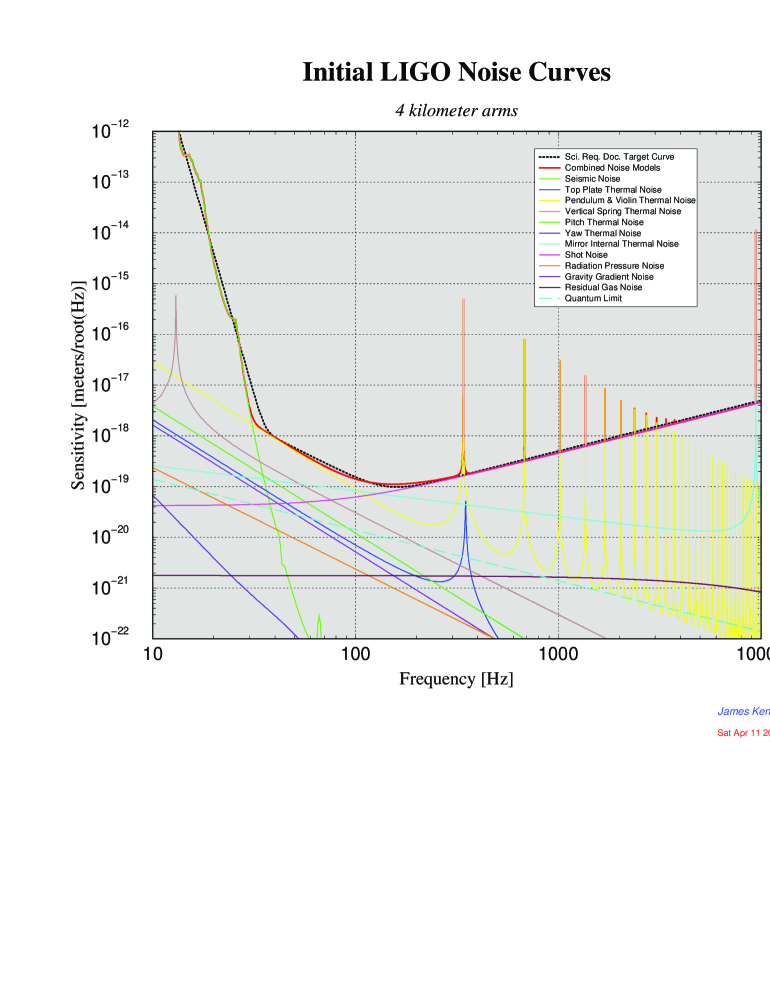
A great effort is being presently devoted to the construction of large scale interferometers. The Laser Interferometer Gravitational-Wave Observatory (LIGO) is being developed by an MIT-Caltech collaboration. LIGO [4] consists of two widely separated interferometers, in Hanford, Washington, and in Livingston, Louisiana. The commissioning of the detectors will begin in 2000, and the first data run is expected to begin in 2002 [31]. The arms of both detectors will be 4 km long; in Hanford there will be also a second 2 km interferometer implemented in the same vacuum system. The sensitivity of the 4 km interferometers is shown in fig. 1. The sensitivity is here given in meters per root Hz; to obtain $\tilde{h}_{f}$, measured in $1/\sqrt{{\rm Hz}}$, one must divide by the arm length in meters, i.e. by 4000. The sensitivity in $1/\sqrt{\rm Hz}$ is shown in fig. 5, next subsection, together with the sensitivity of advanced LIGO. The LIGO interferometer already has a 40m prototype at Caltech, which has been used to study sensitivity, optics, control, and even to do some work on data analysis [9].

Figure 1: The planned LIGO sensitivity curve, in meters$/\sqrt{{\rm Hz}}$ (courtesy of the LIGO collaboration).

A comparable interferometer is VIRGO [69, 256, 53] which is being built by an Italian-French collaboration supported by INFN and CNRS, with 3 km arm length, and is presently under construction in Cascina, near Pisa. These experiments are carried out by very large collaborations, comparable to the collaborations of particle physics experiments. For instance, VIRGO involves about 200 people. Fig. 2 shows, in terms of $\tilde{h}_{f}$, the expected sensitivity of the VIRGO interferometer. By the year 2000 it should be possible to have the first data from a 7 meters prototype, which will be used to test the suspensions, vacuum tube, etc.

Interferometers are wide-band detectors, that will cover the region between a few Hertz up to approximately a few kHz. Figs. (1,2) show separately the main noise sources. At very low frequencies, $f<2$ Hz for VIRGO and $f<40$ Hz for LIGO, the seismic noise dominates and sets the lower limit to the frequency band. Above a few Hz, the VIRGO superattenuator reduces the seismic noise to a neglegible level. Then, up to a few hundreds Hz, thermal noise dominates, and finally the laser shot noise takes over. The various spikes are mechanical resonances due to the thermal noise: first, in fig. 2, the high frequency tail of the pendulum mode (in this region LIGO is still dominated by seismic noise), then a series of narrow resonances due to the violin modes of the wires; finally, the two rightmost spikes in the figures are the low frequency tail of the resonances due to internal modes of the two mirrors. All resonances appear in pairs, at frequencies close but non-degenerate, because the two mirrors have different masses. The width of these spikes is of the order of fractions of Hz. Note that the clustering of the various resonances in the kHz region is due to the logarithmic scale in figs. (1,2). The resonances are actually evenly spaced and narrow, so that in this frequency range the relevant curve is mostly the one given by the shot noise.

Figure 2: The planned VIRGO sensitivity curve (from ref. [16]).

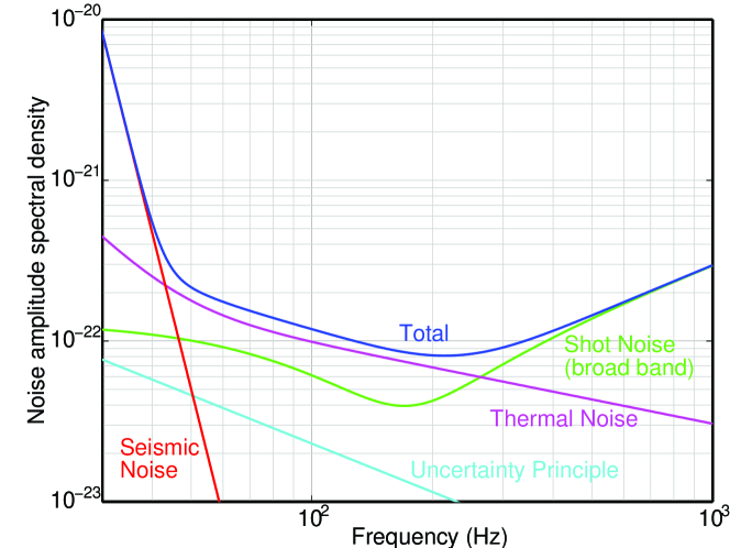
Under construction is also GEO600 [185], a collaboration between the Max-Planck-Institut für Quantenoptik in Garching and the University of Glasgow. It is being built near Hannover, with arms 600 meters in length. GEO600 is somewhat smaller than LIGO and VIRGO, but will use techniques that will be important for the advanced detectors. In particular, the signal recycling of GEO600 provides an opportunity to change the spectral characteristics of the detector response, especially those due to the shot noise limitation, therefore in the high frequency range of the available bandwidth. By choosing low or high mirror reflectivities for the signal-recycling mirror, one can use the recycling either to distribute the improvement in the sensitivity on a wideband, or to improve it even further on a narrow band. This is the so-called narrow-banding of an interferometer. The sensitivity of GEO600 broad-band is shown in fig. 3, and with narrow-banding at 600 Hz in fig. 4.

Figure 3: The planned GEO sensitivity curve, without narrow-banding (courtesy of the GEO collaboration).

Figure 4: The planned GEO sensitivity curve, with narrow-banding at 600 Hz (courtesy of the GEO collaboration).

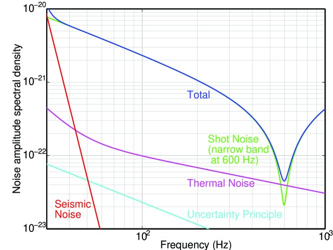
The frequency of maximum sensitivity is tunable to the desired value by shifting the signal-recycling mirror, and thus changing the resonance frequency of the signal-recycling cavity. In its tunable narrowband mode, GEO600 might well be able to set the most stringent limits of all for a while.

TAMA300 (Japan) [163] is the other large interferometer. It is a five year project (1995-2000) that aims to develop the advanced techniques that will be needed for second generation experiments, and catch GWs that may occur by chance within out local group of galaxies. Its has 300 meters arm length. It is hoped that the project will evolve into the proposed Laser Gravitational Radiation Telescope (LGRT), which should be located near the SuperKamiokande detector.

Furthermore, Australian scientists have joined forces to form the Australian Consortium for Interferometric Gravitational Astronomy (ACIGA) [227]. A design study and research with particular emphasis on an Australian detector is nearing completion. The detector, AIGO, will be located north of Perth. Its position in the southern emisphere will greatly increase the baseline of the worldwide array of detectors, and it will be close to the resonant bar NIOBE so that correlations can be performed. The detector will use sapphire optics and sapphire test masses, a material that LIGO plans to use only in its advanced stage, see sect. 5.2

All these detectors will be used in a worldwide network to increase the sensitivity and the reliability of a detection.

Using the values of $\tilde{h}_{f}$ given in the figures and the value $1/F=2.5$ for interferometers, we see from eq. (54) that VIRGO, GEO600 or any of the two LIGOs , used as single detectors, can reach a minimum detectable value for $h_{0}^{2}\Omega_{\rm gw}$ of order $10^{-2}$ or at most a few times $10^{-3}$, at $f=$ 100Hz. Unfortunately, at this level current theoretical expectations exclude the possibility of a cosmological signal, as we will discuss in sect. 7 and 8. As we will see, an interesting sensitivity level for $h_{0}^{2}\Omega_{\rm gw}$ should be at least of order $10^{-6}$. To reach such a level with a single interferometer we need, e.g.,

$$\tilde{h}_{f}(f=100\,{\rm Hz})<10^{-24}\,\,{\rm Hz}^{-1/2}\,,$$ (93)

or

$$\tilde{h}_{f}(f=1\,{\rm kHz})<3\times 10^{-26}\,{\rm Hz}^{-1/2}\,.$$ (94)

We see from the figures that such small values of $\tilde{h}_{f}$ are very far from the sensitivity of first generation interferometers, and are in fact even well below the limitation due to quantum noise. Of course, one should stress that theoretical prejudices, however well founded, are no substitute for a real measurement, and that even a negative result at the level $h_{0}^{2}\Omega_{\rm gw}\sim 10^{-2}$ would be interesting.

5.2 Advanced LIGO

It is important to have in mind that the interferometers discussed in the previous section are the first generation of large scale interferometers, and in this sense they represent really a pioneering effort. At the level of sensitivity that they will reach, they have no guaranteed source of detection. However, they will open the way to second generation interferometers, with much better sensitivity. GEO600 and TAMA300 are important for testing the technique that will be needed for second generation experiments, while the larger interferometers VIRGO and LIGOs should evolve into second generation experiments.

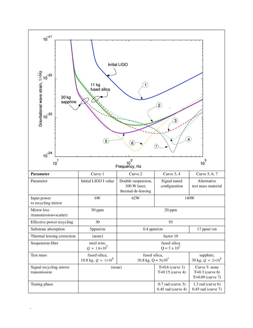
The LIGO collaboration has presented a recommended program for research and developement, that will lead to the Advanced LIGO project [177]. The results are shown in fig. 5, together with the changes in a number of parameters that are responsible for the various improvements shown in the figure.

Figure 5: The planned advanced LIGO sensitivity curves, and the parameters relative to the various improvements, from ref. [177] (courtesy of the LIGO collaboration).

The improvement program is divided into three stages: LIGOII near term, LIGOII medium term and LIGOIII.

Curve 1 in fig. 5 shows the sensitivity of LIGOI, while LIGOII near term is shown in curve 2. The changes leading to LIGOII near term should be incorporated by the end of 2004, and are based on engeneering developents of existing technology or modest stretches from present day systems. They would result in significant improvements of the sensitivity, and are also necessary to gain full advantage of subsequent changes. In particular, a significant reduction in thermal noise will be obtained using fused silica fibers in the test mass suspension; a moderate improvement in seismic isolation will move the seismic noise below this new thermal noise floor, and an increase in the laser power to $\sim 100$ watts results in a decrease of shot noise.

The goal of the medium term program are more ambitious technically, and it is estimated that they could be incorporated in LIGO by the end of 2006. They include signal recycling. As discussed above, this could be used either to obtain a broad-band redistribution of sensitivity (curve 3), or to improve the sensitivity in some narrow band (curve 4).

Another possible improvement is the change of the test masses from fused silica to sapphire or other similar materials. Sapphire has higher density and higher quality factor, and this should result in a significant reduction in thermal noise. For an optical configuration without recycling, the sensitivity is given by curve 5. With signal recycling, possible responses are shown in curves 6 and 7. These changes require significant advances in material technology, and so are considered possible but ambitious for LIGOII.

Fig. 5 does not show performances for LIGOIII detectors, which are expected to provide possibly another factor of 10 of improvement in $\tilde{h}_{f}$, but of course are quite difficult to predict reliably at this stage.

The overall improvement of LIGOII can be seen to be, depending on the frequency, one or two orders of magnitude in $\tilde{h}_{f}$. This is quite impressive, since two order of magnitudes in $\tilde{h}_{f}$ means four order of magnitudes in $h_{0}^{2}\Omega_{\rm gw}(f)$ and therefore an extremely interesting sensitivity, even for a single detector, without correlations.

5.3 The space interferometer LISA

The space interferometer LISA [36, 95, 150] was proposed to the European Space Agency (ESA) in 1993, in the framework of ESA’s long-term space science program Horizon 2000. The original proposal involved using laser interferometry beteween test masses in four drag-free spacecrafts placed in a Heliocentric orbit. In turn, this led to a proposal for a six spacecrafts mission, which has been selected by the European Space Agency has a cornerstone mission in its future science program Horizon 2000 Plus. This implies that in principle the mission is approved and that funding for industrial studies and technology developement is provided right away. The launch year however depends on the availability of fundings. With reasonable estimates it is then expected that it will not be launched before 2017, and possibly as late as 2023. In Feb. 1997 the LISA team and ESA’s Fundamental Physics Advisory Group proposed to carry out LISA in collaboration with NASA. If approved, this could make possible to launch it between 2005-2010. The design has also been somewhat simplified, with three drag-free spacecrafts. The spacecrafts will be in a Heliocentric orbit, at a distance of 1 AU from the Sun, 20 degrees behind the Earth. This design has lower costs, and it is likely to be adopted for future studies relevant to the project [150]. The mission is planned for two years, but it could last up to 10 years without exausting on-board supplies.

LISA has three arms, first of all for redundancy. Thus, it can be thought of as two interferometers sharing a common arm. Of course, this means that the two interferometers will have a common noise. However, most signals are expected to have a signal-to-noise ratio so high that the noise will be neglegible. Then, the output from the two interferometers can be used to obtain extra informations on the polarization and direction of a GW. For the stochastic background, the third arm will help to discriminate backgrounds as those produced by binaries or by cosmological effects from anomalous instrumental noise [36].

Goint into space, one is not limited anymore by seismic and gravity-gradient noises; LISA could then explore the very low frequency domain, $10^{-4}$ Hz $<f<1$ Hz. At the same time, there is also the possibility of a very long path length (the mirrors will be freely floating into the spacecrafts at distances of $5\times 10^{6}$ km from each other!), so that the requirements on the position measurment noise can be relaxed. The goal is to reach a strain sensitivity [36]

$$\tilde{h}_{f}=4\times 10^{-21}\,\,{\rm Hz}^{-1/2}$$ (95)

at $f=1$ mHz. At this level, one expects first of all signals from galactic binary sources, extra-galactic supermassive black holes binaries and super-massive black hole formation.

Concerning the stochastic background, eq. (54) shows clearly the advantage of going to low frequency: the factor $f^{3}$ in eq. (54) gives an extremely low value for the minimum detectable value of $h_{0}^{2}\Omega_{\rm gw}$. The sensitivity of eq. (95) would correspond to

$$h_{0}^{2}\Omega_{\rm gw}(f=1\,{\rm mHz})\simeq 1\times 10^{-12}\,.$$ (96)

Since LISA cannot be correlated with any other detector, to have some confidence in the result it is necessary to have a SNR sufficiently large. Certainly one cannot work at SNR=1.65, as we will do when considering the correlation between two detectors. The standard choice made by the LISA collaboration is SNR=5, and eq. (96) refers to this choice. Note that the minimum detectable value of $h_{0}^{2}\Omega_{\rm gw}$ is proportional to (SNR)², since this SNR refers to the amplitude, and $h_{0}^{2}\Omega_{\rm gw}(f)\sim h_{c}^{2}(f)$. Furthermore, eq. (96) takes into account the angles between the arms, $\alpha=60^{o}$, and the effect of the motion of LISA, which together results in a loss of sensitivity by a factor approximately equal to $1/\sqrt{5}$. Eq. (96) shows that LISA could reach a truly remarkable sensitivity in $h_{0}^{2}\Omega_{\rm gw}$.

LISA will have its best sensitivity between 3 and 30 mHz. Above 30 mHz, the sensitivity degrades because the wavelength of the GW becomes shorter than twice the arm-length of $5\times 10^{6}$ km. At low frequencies, instead, the noise curve rises because of spurious forces on the test masses. At some frequency below 0.1 mHz the accelerometer noise will increase rapidly, and the instrumental uncertainty would increase even more rapidly with decreasing frequency, setting a lower limit to the frequency band of LISA.

Figure 6: The sensitivity of LISA to a stochastic background of GWs after one year of observation, and SNR=5 (from ref. [36]; courtesy of the LISA collaboration).

Figure 7: The sensitivity of LISA for periodic sources, and of advanced LIGO for burst sources, together with some expected astrophysical signals (from ref. [36]; courtesy of the LISA collaboration).

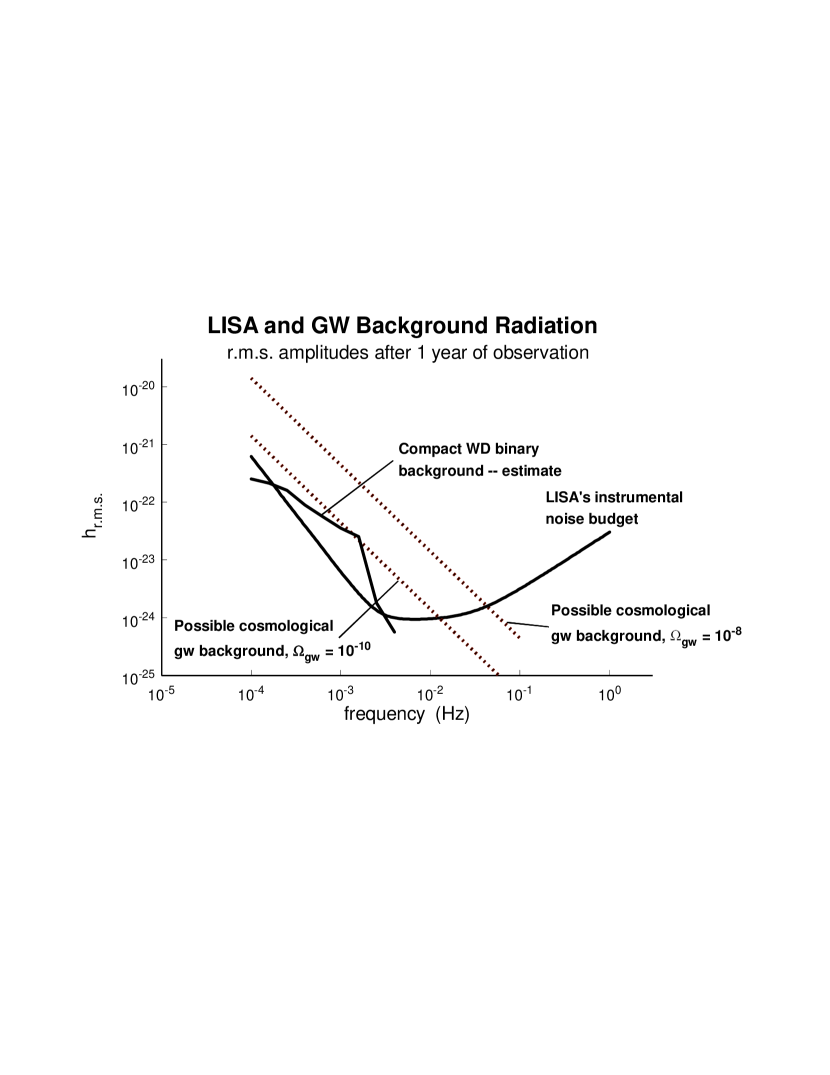
Below a few mHz it is expected also a stochastic background due to compact white-dwarf binaries, that could cover a cosmological background. The sensitivity curve of LISA to a stochastic background, together with the estimated white-dwarf binaries background, is shown in fig. 6. On the vertical axis is shown $h_{\rm r.m.s.}\equiv h_{c}(f,\Delta f=3\times 10^{-8}\,{\rm Hz})$, defined in eq. (23), which is written in [36] in the equivalent form

$$h_{c}(f,\Delta f=3\times 10^{-8}\,{\rm Hz})=5.5\times 10^{-22}\left(\frac{\Omega_{\rm gw}}{10^{-8}}\right)^{1/2}\left(\frac{1\,{\rm mHz}}{f}\right)^{3/2}\left(\frac{H_{0}}{75\,{\rm km\,s}^{-1}\,{\rm Mpc}^{-1}}\right)\,.$$ (97)

Two lines of constant $\Omega_{\rm gw}$, equal to $10^{-10}$ and $10^{-8}$, are also shown in the figure.

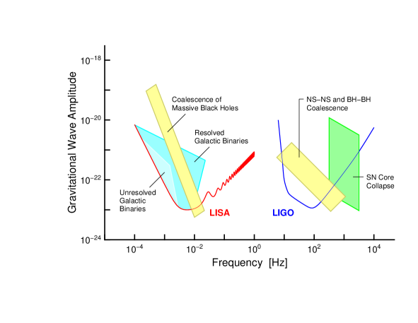
To compare with interferometers, fig. 7 shows the sensitivity to the GW amplitude for both LISA and the advanced LIGO, together with a number of signals expected from astrophysical sources. It is apparent from the figure that ground-based and space-borne interferometers are complementary, and together can cover a large range of frequencies, and, in case of a detection of a cosmological signal, together they can give crucial spectral informations.

The sensitivities shown are presented by the collaboration as conservatives because [36]

1. The errors have been calculated realistically, including all substantial error sources that have been thought of since early studies of drag-free systems, and since the first was flown over 25 years ago, and in most cases (except shot noise) the error allowance is considerably larger than the expected size of the error and is more likely an upper bound.

2. LISA is likely to have a significantly longer lifetime than one year, which is the value used to compute these sensitivities.

3. The sensitivity shown refers only to one interferometer. Using three arms could increase the SNR by perhaps 20% .

An interesting feature of LISA is that, as it rotates in its orbit, its sensitivity to different directions changes. Then, LISA can test the isotropy of a stochastic background. This can be quite important to separate a cosmological signal from a stochastic background of galactic origin, which is likely to be concentrated on the galactic plane. By comparing two 3-month stretches of data, LISA should have no difficulty in identifying this effect. Furthermore, if the mission lasts 10yr, LISA will be close to the sensitivity needed to detect the dipole anisotropy in a cosmological background due to the motion of the solar system. If the GW background turned out not to have the same dipole anisotropy as the cosmic microwave background, one would have found evidence for anisotropic cosmological models.

5.4 Resonant bars: NAUTILUS, EXPLORER, AURIGA, ALLEGRO, NIOBE

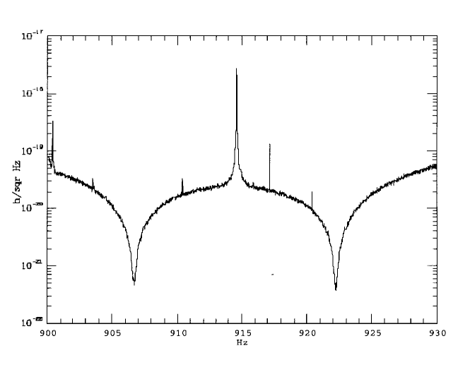
Cryogenic resonant antennas have been taking date since 1990 (see e.g. ref. [215] for review). Fig. 8 shows the sensitivity of NAUTILUS [17, 18, 19, 79], the resonant bar located in Frascati, near Rome. It is an ultracryogenic detector, operating at a temperature $T=0.1$ K. This figure is based on a two hour run, but the behaviour of the apparatus is by now quite stationary over a few days, with a duty cycle limited to 85% by cryogenic operations. Compared to the interferometers, we see that bars are narrow-band detectors, and work at two resonances. The bandwidth is limited basically by the noise in the amplifier. The value of the resonance can be slightly tuned, at the level of a few Hz, working on the electronics. In the figure, the resonances are approximately at 907 Hz and 922 Hz, with half-height bandwiths of about 1 Hz. At these frequencies the strain sensitivity is

$$\tilde{h}_{f}\simeq 5\times 10^{-22}\,,$$ (98)

about a factor of 5 higher than the sensitivity of the interferometers at the same frequencies.

With a thermodynamic temperature of 0.1 K, the experimental data are in very good agreement with a gaussian distribution, whose variance gives an effective temperature $T_{\rm eff}=4.1$ mK. The effective temperature $T_{\rm eff}$ is related to the thermodynamic temperature $T$ by $T_{\rm eff}\simeq 4T\Gamma^{1/2}$, where $\Gamma$ is inversely proportional to the quality factor $Q$ of the resonant mode, so that $\Gamma\ll 1$.

With improvements in the electronics, the collaboration plans to reach in a few years the target sensitivity

$$\tilde{h}_{f}\simeq 8.6\times 10^{-23}\,{\rm Hz}^{-1/2}\,,$$ (99)

and $T_{\rm eff}\sim 10\mu$K, over a bandwidth of 10 Hz [18, 19].

Figure 8: The sensitivity curve of NAUTILUS (courtesy of the NAUTILUS collaboration)

The cryogenic resonant bar EXPLORER [208] is in operation at Cern since 1990, cooled at a temperature $T=2.9$ K, and has taken data at approximately the same frequencies as NAUTILUS, 905 and 921 Hz; its sensitivity is approximately the same as NAUTILUS.

Similar sensitivities are obtained by ALLEGRO, (Louisiana) [193, 142]. ALLEGRO has been taking data since 1991. The resonances are at 897 and 920 Hz.

The resonant bar NIOBE [45, 46, 144, 145] is located in Perth, Australia, and it has operated since 1993. The resonant frequencies are at 694.6 Hz and 713 Hz. It is made of niobium, instead of aluminium as the other bars, since it has a higher mechanical quality factor. This has allowed to reach a noise temperature of less then 2mK, while the typical noise temperature is around 3mK. Improvement in the transducer system should allow to lower $T_{\rm eff}$ to a few microkelvin, in a bandwidth of 70 Hz. This would allow to reach a sensitivity comparable to interferometers over a large bandwidth, approximately 650-750 Hz [145].

AURIGA [72, 218, 219] is located in Legnaro, near Padua, Italy. It began full operations in 1997. The bar is cooled at 0.2K, and the effective temperature is $T_{\rm eff}=7$ mK. The resonances are at 911 and 929 Hz. The spectral sensitivity reached [219] is similar to that of NAUTILUS.

All these bars are designed to operate in a well coordinated way, in order to improve the chances of reliable detection.

From eq. (99) we see that, without performing correlations between different detectors, the sensitivity that one could get from resonant bars is between at most $h_{0}^{2}\Omega_{\rm gw}^{\rm min}(f)\sim O(1)$ and $h_{0}^{2}\Omega_{\rm gw}^{\rm min}(f)\sim O(10)$ and therefore quite far from a level where one can expect a cosmological signal. In sect. 6 we will discuss the level that can be reached with correlations between bars, and between a bar and an interferometer.

5.5 Some projects at a preliminary stage

A number of other projects for gravitational wave detection have been put forward and are presently at the stage of testing prototypes.

An especially interesting project involves resonant mass detectors with truncated icosahedron geometry [157, 198, 199, 80, 42, 238]. A spherical detector, in fact, has a larger mass compared to a bar with the same resonance frequency, and therefore a larger cross section. Furthermore, it has the informations about the directions and polarization of a GW that could only be obtained with 5 different resonant bars. The problem of attaching mechanical resonators to the detector suggests a truncated icosahedral geometry, rather than a sphere.

A prototype called TIGA (Truncated Icosahedral Gravitational Wave Antenna) has been built at the Lousiana State University [198]. It has its first resonant mode at 3.2 kHz. The Rome group has started the SFERA project [25]. A working group has been formed to to carry out studies and measurements in order to define a project of a large spherical detector, 40 to 100 tons of mass, competitive with large interferometers but with complementary features. A correlation between an interferometer and a sphere could in particular have quite interesting sensitivities for the stochastic background.

These spheres could reach approximately one order of magnitude better in the sensitivity $\tilde{h}_{f}$ [80, 182] compared to resonant bars. Furthermore, they have different channels, see eqs. (3.1.3) and (3.1.3), that are sensitive to different spin content [118, 259, 157]. This would allow to discriminate between different theories of gravity, separating for instance the effects of scalar GWs, which could originate from a Brans-Dicke theory [258, 159, 182, 54, 42, 206, 189]. Scalars fields originating from string theory, as the dilaton and the moduli of compactifications, are however a much more difficult target: to manifest themselves as coherent scalar GWs they should be extremely light, $m<10^{-12}$ eV [189]. Actually, there is the possibility to keep the dilaton and moduli fields extremely light or even massless, with a mechanism that has been proposed by Damour and Polyakov [94]. In fact, assuming some form of universality in the string loop corrections, it is possible to stabilize a massless dilaton during the cosmological evolution, at a value where it is essentially decoupled from the matter sector. In this case, however, the dilaton becomes decoupled also from the detector, since the dimensionless coupling of the dilaton to matter ($\alpha$ in the notation of [94]) is smaller than $10^{-7}$ (see also [92]). Such a dilaton would then be unobservable at VIRGO, although it could still produce a number of small deviations from General Relativity which might in principle be observable improving by several orders of magnitude the experimental tests of the equivalence principle [90].

Recently, hollow spheres have been proposed in ref. [78]. The theoretical study suggests a very interesting value for the strain sensitivity, even of order

$$\tilde{h}_{f}\sim\,{\rm a\,few}\times 10^{-24}\,.$$ (100)

The resonance frequency, depending on the material used and other parameters, can be between approximately 200 Hz and 1-2 kHz, and the bandwidth can be of order 20 Hz.

Another idea which is discussed is an array of resonant masses [119, 120, 111], each with a different frequency $f$, and a bandwidth $\Delta f\sim f/10$, which together would cover the region from below the kHz up to a few kHz.

Although not of immediate applicability to GW search, we finally mention the proposal of using two coupled superconducting microwave cavities to detect very small displacements. The idea goes back to the works [211, 212, 213, 71, 153]. These detectors have actually been constructed in ref. [221], using two coupled cavities with frequencies of order of 10GHz; the coupling induces a shift in the levels of order of 1 MHz, and transitions between these levels could in principle be induced by GWs. However, eq. (54) shows clearly the problem with working at such a high frequency, $f\sim 1$ MHz: to reach an interesting value for $h_{0}^{2}\Omega_{\rm gw}(f)$ of order $10^{-6}$, one needs $\tilde{h}_{f}\sim 10^{-30}$ Hz^-1/2, very far from present technology. There is however the proposal [40] to repeat the experiment with improved sensitivity, so to reach $\tilde{h}_{f}\sim 6\times 10^{-24}$ Hz^-1/2 at $f=1$ MHz, and, if this should work, then one would try to lower the resonance frequency down to, possibly, a few kHz. This second step would mean to move toward much larger cavities, say of the kind used at LEP.

6 Sensitivity of various two-detectors correlations

In the previous section we have seen that with a single detector (and with the exception of LISA) we cannot reach sensitivities interesting for cosmological backgrounds of GWs. On the other hand, we have found in sects. (4.3) and (4.4) that many orders of magnitudes can be gained correlating two detectors. In this section we examine the sensitivities for various two-detector correlations.

It is also important to stress that performing multiple detector correlations is crucial not only for improving the sensitivity, but also because in a GW detector there are in general noises which are non-gaussian, and can only be eliminated correlating two or more detectors. An example of a non-gaussian noise in an interferometer is the creep, i.e. the sudden energy release in the superattenuator chain, and most importantly in the wires holding the mirrors, and due to accumulated internal stresses in the material. Indeed, it is feared that this and similar non-stochastic noises might turn out to be the effective sensitivity limit of interferometers, possibly exceeding the design sensitivity [98]. Some sources of non-stochastic noises have been identified, and there are technique for neutralizing or minimizing them. However, it is impossible to guarantee that all possible sources of non-stochastic noises have properly been taken into account, and only the cross correlation between different detectors can provide a reliable GW detection.

6.1 An ideal two-interferometers correlation

We now discuss the sensitivities that could be obtained correlating the major interferometers.

In order to understand what is the best result that could be obtained with present interferometer technology, we first consider the sensitivity that could be obtained if one of the interferometers under constructions were correlated with a second identical interferometer located at a few tens of kilometers from the first, and with the same orientation. This distance would be optimal from the point of view of the stochastic background, since it should be sufficient to decorrelate local noises like, e.g., the seismic noise and local electromagnetic disturbances, but still the two interferometers would be close enough so that the overlap reduction function does not cut off the high frequency range. For this exercise we use the data for the sensitivity of VIRGO, fig. 2.

Let us first give a rough estimate of the sensitivity using $h_{c}(f),h_{n}(f)$. From fig. 2 we see that we can take, for our estimate, $\tilde{h}_{f}\sim 10^{-22}{\rm Hz}^{-1/2}$ over a bandwidth $\Delta f\sim$ 1 kHz. Using $T=$ 1 yr, eq. (88) gives

$$h_{n}(f)\sim 4.5\times 10^{-24}\left(\frac{f}{100{\rm Hz}}\right)^{1/2}\left(\frac{\tilde{h}_{f}}{10^{-22}{\rm Hz}^{-1/2}}\right)\,.$$ (101)

We require for instance SNR=1.65 (this corresponds to $90\%$ confidence level; a more precise discussion of the statistical significance, including the effect of the false alarm rate can be found in ref. [12]). Then the minimum detectable value of $h_{c}(f)$ is $h_{c}^{\rm min}(f)=1.65h_{n}(f)$, and from eq. (19) we get an estimate for the minimum detectable value of $h_{0}^{2}\Omega_{\rm gw}(f)$,

$$h_{0}^{2}\Omega_{\rm gw}^{\rm min}(f)\sim 3\times 10^{-7}\left(\frac{f}{100{\rm Hz}}\right)^{3}\left(\frac{\tilde{h}_{f}}{10^{-22}{\rm Hz}^{-1/2}}\right)^{2}\,.$$ (102)

This suggests that correlating two VIRGO interferometers we can detect a relic spectrum with $h_{0}^{2}\Omega_{\rm gw}({\rm 100Hz})\sim 3\times 10^{-7}$ at SNR=1.65, or $1\times 10^{-7}$ at SNR=1. Compared to the case of a single interferometer with SNR=1, eq. (54), we gain five orders of magnitude. As already discussed, to obtain a precise numerical value one must however resort to eq. (79). This involves an integral over all frequencies, (that replaces the somewhat arbitrary choice of $\Delta f$ made above) and depends on the functional form of $h_{0}^{2}\Omega_{\rm gw}(f)$. If for instance $h_{0}^{2}\Omega_{\rm gw}(f)$ is independent of the frequency, using the numerical values of $\tilde{h}_{f}$ plotted in fig. 2 and performing the numerical integral, we have found for the minimum detectable value of $h_{0}^{2}\Omega_{\rm gw}$

$$h_{0}^{2}\Omega_{\rm gw}^{\rm min}\simeq 2\times 10^{-7}\left(\frac{\rm SNR}{1.65}\right)^{2}\left(\frac{1\rm yr}{T}\right)^{1/2}\hskip 42.67912pt(h_{0}^{2}\Omega_{\rm gw}(f)={\rm const.})\,.$$ (103)

This number is quite consistent with the approximate estimate (102), and with the value $2\times 10^{-7}$ reported in ref. [83]. Stretching the parameters to SNR=1 ($68\%$ c.l.) and $T=4$ years, the value goes down at $(3-4)\times 10^{-8}$. This might be considered an absolute (and quite optimistic) upper bound on the capabilities of first-generation experiments.

It is interesting to note that the main contribution to the integral comes from the region $f<$ 100 Hz. In fact, neglecting the contribution to the integral of the region $f>$ 100 Hz, the result for $h_{0}^{2}\Omega_{\rm gw}^{\rm min}$ changes only by approximately $2\%$. Also, the lower part of the accessible frequency range is not crucial. Restricting for instance to the region 20 Hz $\leq f\leq$ 200 Hz, the sensitivity on $h_{0}^{2}\Omega_{\rm gw}$ degrades by less than $1\%$, while restricting to the region 30 Hz $\leq f\leq$ 100 Hz, the sensitivity on $h_{0}^{2}\Omega_{\rm gw}$ degrades by approximately $10\%$. Then, from fig. 2 we conclude that by far the most important source of noise for the measurement of a flat stochastic background is the thermal noise. In particular, the sensitivity to a flat stochastic background is limited basically by the mirror thermal noise, which dominates in the region 40 Hz$\raise 1.72218pt\hbox{$<$}\kern-8.00003pt\lower 2.6694pt\hbox{$\sim$}f\raise 1.72218pt\hbox{$<$}\kern-8.00003pt\lower 2.6694pt\hbox{$\sim$}200$ Hz, while the pendulum thermal noise dominates below approximately 40 Hz.

The sensitivity depends however on the functional form of $\Omega_{\rm gw}(f)$. Suppose for instance that in the VIRGO frequency band we can approximate the signal as

$$\Omega_{\rm gw}(f)=\Omega_{\rm gw}({\rm 1kHz})\left(\frac{f}{\rm 1kHz}\right)^{\alpha}\,.$$ (104)

For $\alpha=1$ we find that the spectrum is detectable at SNR=1.65 if $h_{0}^{2}\Omega_{\rm gw}({\rm 1kHz})\simeq 3.6\times 10^{-6}$. For $\alpha=-1$ we find (taking $f=$ 5Hz as lower limit in the integration) $h_{0}^{2}\Omega_{\rm gw}({\rm 1kHz})\simeq 6\times 10^{-9}$. Note however that in this case, since $\alpha<0$, the spectrum is peaked at low frequencies, and $h_{0}^{2}\Omega_{\rm gw}(5{\rm Hz})\simeq 1\times 10^{-6}$. So, both for increasing or decreasing spectra, to be detectable $h_{0}^{2}\Omega_{\rm gw}$ must have a peak value, within the VIRGO band, of order a few $\times 10^{-6}$ in the case $\alpha=\pm 1$, while a constant spectrum can be detected at the level $2\times 10^{-7}$. Clearly, for detecting increasing (decreasing) spectra, the upper (lower) part of the frequency band becomes more important, and this is the reason why the sensitivity degrades compared to flat spectra, since for increasing or decreasing spectra the maximum of the signal is at the edges of the accessible frequency band, where the interferometer sensitivity is worse.

6.2 LIGO-LIGO

Let us now see what can be done with existing interferometers. The two LIGO detectors are under construction at a large distance from each other, $d\sim 3000$ km. This choice optimizes the possibility of detecting the direction of arrival of GWs from astrophysical sources, but it is not optimal from the point of view of the stochastic background, since the overlap reduction function cuts off the integrand in eq. (78) at a frequency of the order of $1/(2\pi d)$. The overlap function $\gamma(f)$ for the LIGO-LIGO correlation has been computed in ref. [113]. and it has its first zero at $f\simeq 64$ Hz. Furthermore, the arms of the two detectors are not exactly parallel, and therefore $|\gamma(0)|=0.89$ rather than 1.

The sensitivity to a stochastic background for the LIGO-LIGO correlation has been computed in refs. [200, 74, 113, 8, 12]. The result, as we have discussed, depends on the functional form of $h_{0}^{2}\Omega_{\rm gw}$. For $\Omega_{\rm gw}(f)$ independent of $f$, the minimum detectable value is

$$h_{0}^{2}\Omega_{\rm gw}\simeq 5\times 10^{-6}$$ (105)

for the initial LIGO. However, we have seen that second generation interferometers could result in much better sensitivities. The sensitivity of the correlation between two advanced LIGO is estimated in ref. [8] to be

$$h_{0}^{2}\Omega_{\rm gw}\simeq 5\times 10^{-11}\,,$$ (106)

which is an extremely interesting level. These numbers are given at $90\%$ c.l. in [8], and a detailed analysis of the statistical significance is given in [12].

6.3 VIRGO-LIGO, VIRGO-GEO, VIRGO-TAMA

In Fig. 9 we show the overlap reduction functions for the correlation of VIRGO with the other major interferometers. Using these functions, one can compute numerically the integral in eq. (79) and obtain the minimum detectable value of $h_{0}^{2}\Omega_{\rm gw}$. These values are shown in Table 1 (from ref. [29]), together with the value for LIGO-LIGO computed in ref. [8]. All these numbers are at 90% confidence level.

Figure 9: The overlap reduction functions $\gamma(f)$ for the correlation of VIRGO with the other major interferometers (from ref. [29]).

correlation	$h_{0}^{2}\Omega_{\rm gw}$
LIGO-WA*LIGO-LA	$5\times 10^{-6}$
VIRGO*LIGO-LA	$4\times 10^{-6}$
VIRGO*LIGO-WA	$5\times 10^{-6}$
VIRGO*GEO600	$5.6\times 10^{-6}$
VIRGO*TAMA300	$1\times 10^{-4}$

Table 1: The sensitivity of various two-interferometers correlation.

We see that the correlation between VIRGO and any of the two LIGO is suppressed by the overlap reduction function above, say, 30-40 Hz. In the case of the VIRGO-GEO correlation, instead, $\gamma(f)$ cuts the integrand only above say 200 Hz. However, the sensitivity of GEO is below 200 Hz is lower then LIGO, so that the result are basically the same as for VIRGO-LIGO, see Table 1.

To obtain the precise numbers for the sensitivity, of course one has to perform the integral in eq. (79). However, it is easy to have an understanding of the numbers that come out. As we have found in sect. 6.1, the minimum detectable value of $h_{0}^{2}\Omega_{\rm gw}$, using two identical VIRGO detectors, degrades only by less than 10% if, from the full VIRGO bandwidth, we restrict to the region 20 Hz $<f<$ 100 Hz; in this region $|\gamma(f)|$ for the VIRGO-GEO correlation is constant to a good accuracy, and of order 0.1. From eqs. (79) and (18) we see that the minimum detectable value of $h_{0}^{2}\Omega_{\rm gw}$ scales with $\gamma(f)$ as $|\gamma(f)|^{-1}$. Therefore for the VIRGO-GEO correlation we get about a factor of 10 worse than the ideal result (103). Comparing figs. 2 and 4, and recalling that $h_{0}^{2}\Omega_{\rm gw}^{\rm min}\sim\tilde{h}_{f}^{2}$, we see that we lose about another factor of 3 in $h_{0}^{2}\Omega_{\rm gw}$ compared to an ideal VIRGO-VIRGO correlation, so that one gets the estimate

$$h_{0}^{2}\Omega_{\rm gw}^{\rm min}\sim 6\times 10^{-6}\left(\frac{\rm SNR}{1.65}\right)^{2}\left(\frac{1\rm yr}{T}\right)^{1/2}\hskip 42.67912pt(h_{0}^{2}\Omega_{\rm gw}(f)={\rm const.})\,,$$ (107)

quite in agreement with the result of the more accurate computation shown in Table 1.

The situation with the VIRGO-TAMA300 correlation is instead worse, as can be seen from the overlap reduction function and from the value in Table 1.

6.4 VIRGO-Resonant mass and Resonant mass-Resonant mass

The correlation between two resonant bars and between a bar and an interferometer has been considered in refs. [257, 83, 21, 22, 23, 29].

Fig. 10 shows the overlap reduction functions for the correlation between VIRGO and one of the three resonant bars NAUTILUS, EXPLORER, AURIGA. These overlap reduction functions have been computed assuming that the bars have been reoriented so to achieved the maximum correlation with VIRGO, which is technically feasible.

One should also note that there is the danger that one of the spikes due to the violin modes in the VIRGO sensitivity curve comes close to a resonant frequency of the bar; surprisingly, this apparent unlikely event is just what happens with the data used to draw fig. 2; in fact, according to these data there is a pair of violin modes at 922.6 Hz and 977.2 Hz. The first one happens to fall exactly at the resonance at 922 Hz of NAUTILUS! However, these data for the violin modes are not yet final. For instance, the VIRGO collaboration is presently considering the possibility of using silica instead of steel for the wires, which would change the position of the resonances. Furthermore, the resonance frequency of the bars can be tuned within a few Hz with the electronics; this would be quite sufficient, since the violine modes have a very high Q and so are much narrower than one Hz.

The minumum detectable values for $h_{0}^{2}\Omega_{\rm gw}$ for some bar-bar and bar-interferometer correlations are given in Table 2 (from ref. [29]), for one year of observation and 90% confidence level (SNR=1.65).

correlation	$h_{0}^{2}\Omega_{\rm gw}$
VIRGO*AURIGA	$4\times 10^{-4}$
VIRGO*NAUTILUS	$7\times 10^{-4}$
AURIGA*NAUTILUS	$5\times 10^{-4}$

Table 2: The sensitivity of the correlation of VIRGO with resonant bars, and of two resonant bars (from ref. [29]), but setting the confidence level to 90% ).

A three detectors correlation AURIGA-NAUTILUS-VIRGO, with present orientations, would reach

$$h_{0}^{2}\Omega_{\rm gw}\simeq 3\times 10^{-4}\,,$$ (108)

at 90% c.l., while with optimal orientation,

$$h_{0}^{2}\Omega_{\rm gw}\simeq 1.6\times 10^{-4}\,.$$ (109)

Although the improvement in sensitivity in a bar-bar-interferometer correlation is not large compared to a bar-bar or bar-interferometer correlation, a three detectors correlation would be important in ruling out spurious effects [257].

Figure 10: The overlap reduction function $\gamma(f)$ for the correlation of VIRGO with NAUTILUS (solid line), AURIGA (dashed line) and EXPLORER (dotted line) in the case in which the bars have been reoriented so to be aligned with VIRGO (from ref. [29]).

In the case of correlations involving resonant bars, obviously there is no issue of optimal filtering, since they are narrow-band detector, and the sensitivity does not depend on the shape of the spectrum. As we have seen in sect. 5, using resonant optical techniques, it is possible to improve the sensitivity of interferometers at special values of the frequency, at the expense of their broad-band sensitivity. Since bars have a narrow band anyway, narrow-banding the interferometer improves the sensitivity of a bar-interferometer correlation by about one order of magnitude [83]. Thus, the limit of bar-bar-interferometer correlation, with narrow banding of the interferometer, is of order $h_{0}^{2}\Omega_{\rm gw}\sim{\rm a\,few}\times 10^{-5}$.

Cross-correlation experiments have already been performed using NAUTILUS and EXPLORER [24]. The bar are oriented so that they are parallel, and then the overlap reduction function $\Gamma(f)$ results in a reduction of sensitivity of about a factor of 6, compared to ideal same site detectors. The detectors are tuned at the same resonance frequency $f=907.2$ Hz, with an overlapping band $\pm 0.05$ Hz, and the overlapped data cover a period of approximately 12 hours. Of course, with such a short coincidence time, the bound on $h_{0}^{2}\Omega_{\rm gw}$ is not yet significant. Running for one year, it is expected to reach $h_{0}^{2}\Omega_{\rm gw}<1$. Cross-correlations, searching for bursts, have also been done between ALLEGRO and EXPLORER [20]

It is also important to observe that, at the level of sensitivity that we are discussing, the effect of cosmic rays on the resonant detectors can be relevant [13, 82, 194, 26, 216]. For a stochastic background, cosmic rays at sea level degrade the power spectrum sensitivity of a single resonant mass detector by a factor $(20{\rm mK}+T_{\rm eff})/T_{\rm eff}$ [216]. For the coincidence between two resonant masses it would then be useful to place one of the two detectors underground (not much is gained placing both detectors underground). In the coincidence between a resonant mass and an interferometer, instead, this is not necessary, since the interferometer is much less sensitive to cosmic rays.

While resonant bars have been taking data for years, spherical detectors are at the moment still at the stage of theoretical studies (although prototypes might be built in the near future), but could reach extremely interesting sensitivities. In particular, two spheres with a diameter of 3 meters, made of Al5056, and located at the same site, could reach a sensitivity $h_{0}^{2}\Omega_{\rm gw}\sim 4\times 10^{-7}$ [257]. This figure improves using a more dense material or increasing the sphere diameter, but it might be difficult to build a heavier sphere. Another very promising possibility is given by hollow spheres [78]. The theoretical studies of ref. [78] suggest that correlating two hollow spheres one could reach the

$$h_{0}^{2}\Omega_{\rm gw}\simeq 10^{-9}\times\left(\frac{f}{200\,{\rm Hz}}\right)^{3}\left(\frac{\tilde{h_{f}}}{10^{-24}\,{\rm Hz}^{-1/2}}\right)^{2}\left(\frac{20\,{\rm Hz}}{\Delta f}\right)^{1/2}\left(\frac{10^{7}\,{\rm s}}{T}\right)^{1/2}\,.$$ (110)

With the value of $\tilde{h}_{f}$ and $\Delta f$ suggested by ref. [78], it could be possible to reach an extremely interesting value, $h_{0}^{2}\Omega_{\rm gw}\sim 10^{-9}$.

7 Bounds on $h_{0}^{2}\Omega_{\rm gw}(f)$

In this section we discuss various experimental bounds on $h_{0}^{2}\Omega_{\rm gw}(f)$. We will be interested not only on the bounds at values of $f$ where interferometers or resonant bars can operate, but also at all possible frequencies. The reason will become apparent when we will discuss the spectra from various specific cosmological mechanisms for the production of relic GWs. These spectra depend of course on the parameters of the cosmological model. Often the frequency dependence is, to a first approximation, completely determined, but the overall value of $h_{0}^{2}\Omega_{\rm gw}$ depends on some parameters of the model. In some case, and especially for the amplification of vacuum fluctuations (sect. 9.1) these spectra extend over a huge range of frequencies, ranging from frequencies as small as $10^{-18}$ Hz (corresponding to wavelength of the order of the present Hubble radius of the Universe) up to possibly the GHz region. It is therefore important to see what are the experimental constraint, at any frequency, on $h_{0}^{2}\Omega_{\rm gw}$, since they automatically imply bounds on the parameters of the model that enter in the spectrum, and therefore on its the value at frequencies accessible to interferometers or resonant masses.

The various limits discussed in this section are summarized in fig. 11.

Figure 11: The various bounds on $h_{0}^{2}\Omega_{\rm gw}(f)$ discussed in the text.

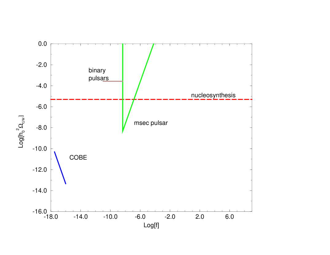
7.1 The nucleosynthesis bound

Nucleosynthesis successfully predicts the primordial abundances of deuterium, ³He, ⁴He and ⁷Li in terms of one cosmological parameter $\eta$, the baryon to photon ratio. In the prediction enter also parameters of the underlying particle theory, which are therefore constrained in order not to spoil the agreement. In particular, the prediction is sensitive to the effective number of species at time of nucleosynthesis, $g_{*}=g(T\simeq{\rm MeV})$. With some simplifications, the dependence on $g_{*}$ can be understood as follows. A crucial parameter in the computations of nucleosynthesis is the ratio of the number density of neutrons, $n_{n}$, to the number density of protons, $n_{p}$, As long as thermal equilibrium is mantained we have (for non-relativistic nucleons, as appropriate at $T\sim$ MeV, when nucleosynthesis takes place) $n_{n}/n_{p}=\exp(-Q/T)$ where $Q=m_{n}-m_{p}\simeq 1.3$ MeV. Equilibrium is mantained by the process $pe\leftrightarrow n\nu$, with width $\Gamma_{pe\rightarrow n\nu}$, as long as $\Gamma_{pe\rightarrow n\nu}>H$. When the rate drops below the Hubble constant $H$, the process cannot compete anymore with the expansion of the Universe and, apart from occasional weak processes, dominated by the decay of free neutrons, the ratio $n_{n}/n_{p}$ remains frozen at the value $\exp(-Q/T_{\rm f})$, where $T_{\rm f}$ is the value of the temperature at time of freeze-out. This number therefore determines the density of neutrons available for nucleosynthesis, and since practically all neutrons available will eventually form ⁴He, the final primordial abundance of ⁴He is exponentially sensitive to the freeze-out temperature $T_{\rm f}$. Let us take for simplicity $\Gamma_{pe\rightarrow n\nu}\sim G_{F}^{2}T^{5}$ (which is really appropriate only in the limit $T\gg Q$). The Hubble constant is given by $H^{2}=(8\pi/3)G\rho$, where $\rho$ includes all form of energy density at time of nucleosynthesis, and therefore also the contribution of primordial GWs. As usual, it is convenient to write the total energy density $\rho$ in terms of $g_{*}$, see eq. (152), as $\rho=(\pi^{2}/30)g_{*}T^{4}$. We recall that, for gravitons, the quantity $T_{i}$ entering eq. (152) is defined by $\rho_{\rm gw}=2(\pi^{2}/30)T_{i}^{4}$, and this does not imply a thermal spectrum. Then the freeze-out temperature $T_{\rm f}$ is determined by the condition

$$G_{F}^{2}T_{\rm f}^{5}\simeq\left(\frac{8\pi^{3}g_{*}}{90}\right)^{1/2}\frac{T_{\rm f}^{2}}{M_{\rm Pl}}\,.$$ (111)

This shows that $T_{\rm f}\sim g_{*}^{1/6}$, at least with the approximation that we used for $\Gamma_{pe\rightarrow n\nu}$. A large energy density in relic gravitons gives a large contribution to the total density $\rho$ and therefore to $g_{*}$. This results in a larger freeze-out temperature, more available neutrons and then in overproduction of ⁴He. This is the idea behind the nucleosynthesis bound [233]. More precisely, since the density of ⁴He increases also with the baryon to photon ratio $\eta$, we could compensate an increase in $g_{*}$ with a decrease in $\eta$, and therefore we also need a lower limit on $\eta$, which is provided by the comparison with the abundance of deuterium and ³He.

Rather than $g_{*}$, it is often used an ‘effective number of neutrino species’ $N_{\nu}$ defined as follows. In the standard model, at $T\sim$ a few MeV, the active degrees of freedom are the photon, $e^{\pm}$, neutrinos and antineutrinos, and they have the same temperature, $T_{i}=T$. Then, for $N_{\nu}$ families of light neutrinos, $g_{*}(N_{\nu})=2+(7/8)(4+2N_{\nu})$, where the factor of 2 comes from the two elicity states of the photon, 4 from $e^{\pm}$ in the two elicity states, and $2N_{\nu}$ counts the $N_{\nu}$ neutrinos and the $N_{\nu}$ antineutrinos, each with their single elicity state; the factor (7/8) holds for fermions. In the Standard Model with $N_{\nu}=3$, $g_{*}=43/4$. So we can define an ‘effective number of neutrino species’ $N_{\nu}$ from

$$\frac{43}{4}+\sum_{i=\rm extra\,bosons}g_{i}\left(\frac{T_{i}}{T}\right)^{4}+\frac{7}{8}\sum_{i=\rm extra\,fermions}g_{i}\left(\frac{T_{i}}{T}\right)^{4}=2+\frac{7}{8}(4+2N_{\nu})\,,$$ (112)

or

$$\sum_{i=\rm extra\,bosons}g_{i}\left(\frac{T_{i}}{T}\right)^{4}+\frac{7}{8}\sum_{i=\rm extra\,fermions}g_{i}\left(\frac{T_{i}}{T}\right)^{4}=\frac{7}{4}(N_{\nu}-3)\,.$$ (113)

One extra species of light neutrino, at the same temperature as the photons, would contribute one unit to $N_{\nu}$, but all species, weighted with their energy density, contribute to $N_{\nu}$, which of course in general is not an integer. For $i=$ gravitons, we have $g_{i}=2$ and $(T_{i}/T)^{4}=\rho_{\rm gw}/\rho_{\gamma}$, where $\rho_{\gamma}=2(\pi^{2}/30)T^{4}$ is the photon energy density. If gravitational waves give the only extra contribution to $N_{\nu}$, compared to the standard model with $N_{\nu}=3$, then

$$\sum_{i=\rm extra\,bosons}g_{i}\left(\frac{T_{i}}{T}\right)^{4}=2\frac{\rho_{\rm gw}}{\rho_{\gamma}}\,,$$ (114)

and therefore

$$\left(\frac{\rho_{\rm gw}}{\rho_{\gamma}}\right)_{\rm NS}=\frac{7}{8}(N_{\nu}-3)\,,$$ (115)

where the subscript NS reminds that this equality holds at time of nucleosynthesis. If more extra species, not included in the standard model, contribute to $g_{*}(N_{\nu})$, then the equal sign in the above equation is replaced by lower or equal. The same happens if there is a contribution from any other form of energy present at the time of nucleosynthesis and not included in the energy density of radiation, like, e.g., primordial black holes.

To obtain a bound on the energy density at the present time, we note that from the time of nucleosynthesis to the present time $\rho_{\rm gw}$ scaled as $1/a^{4}$, while the photon temperature evolved following $g_{S}(T)T^{3}a^{3}=$ const. (i.e. constant entropy) and $\rho_{\gamma}\sim T^{4}\sim 1/(a^{4}g_{S}^{4/3})$. Therefore

$$\left(\frac{\rho_{\rm gw}}{\rho_{\gamma}}\right)_{0}=\left(\frac{\rho_{\rm gw}}{\rho_{\gamma}}\right)_{\rm NS}\left(\frac{g_{S}(T_{0})}{g_{S}({\rm 1\,MeV})}\right)^{4/3}=\left(\frac{\rho_{\rm gw}}{\rho_{\gamma}}\right)_{\rm NS}\left(\frac{3.913}{10.75}\right)^{4/3}\,,$$ (116)

where the subscript zero denotes present time. Therefore we get the nucleosynthesis bound at the present time,

$$\left(\frac{\rho_{\rm gw}}{\rho_{\gamma}}\right)_{0}\leq 0.227(N_{\nu}-3)\,.$$ (117)

Of course this bound holds only for GWs that were already produced at time of nucleosynthesis ($T\sim$ MeV, $t\sim$ sec). It does not apply to any stochastic background produced later, like backgrounds of astrophysical origin. Note that this is a bound on the total energy density in gravitational waves, integrated over all frequencies. Writing $\rho_{\rm gw}=\int d(\log f)\,d\rho_{\rm gw}/d\log f$, multiplying both $\rho_{\rm gw}$ and $\rho_{\gamma}$ in eq. (117) by $h_{0}^{2}/\rho_{c}$ and inserting the numerical value $h_{0}^{2}\rho_{\gamma}/\rho_{c}\simeq 2.481\times 10^{-5}$ [209], we get

$$\int_{f=0}^{f=\infty}d(\log f)\,\,h_{0}^{2}\Omega_{\rm gw}(f)\leq 5.6\times 10^{-6}(N_{\nu}-3)\,.$$ (118)

The bound on $N_{\nu}$ from nucleosynthesis is subject to various systematic errors in the analysis, which have to do mainly with the issues of how much of the observed ⁴He abundance is of primordial origin, and of the nuclear processing of ³He in stars, and as a consequence over the last five years have been quoted limits on $N_{\nu}$ ranging from 3.04 to around 5. The situation has been reviewed in ref. [89]. The conclusions of ref. [89] is that, until current astrophysical uncertainties are clarified, $N_{\nu}<4$ is a conservative limit. Using extreme assumptions, a meaningful limit $N_{\nu}<5$ still exists, showing the robustness of the argument. Correspondingly, the right-hand side of eq. (118) is, conservatively, of order $5\times 10^{-6}$ and anyway cannot exceed $10^{-5}$.

If the integral cannot exceed these values, also its positive definite integrand $h_{0}^{2}\Omega_{\rm gw}(f)$ cannot exceed it over an appreciable interval of frequencies, $\Delta\log f\sim 1$. One might still have, in principle, a very narrow peak in $h_{0}^{2}\Omega_{\rm gw}(f)$ at some frequency $f$, with a peak value larger than say $10^{-5}$, while still its contribution to the integral could be small enough. But, apart from the fact that such a behaviour seems rather implausible, or at least is not suggested by any cosmological mechanism, in the detection at broadband detectors like VIRGO, one must also take into account that, even if we gain in the height of the signal, this is partially compensated by the fact that we lose because of the reduction of the useful frequency band $\Delta f$, see eq. (78).

It is sometimes useful to think in terms of the dimensionless amplitude $h_{c}(f)$ instead of $h_{0}^{2}\Omega_{\rm gw}$. From eq. (19), we see that a bound $h_{0}^{2}\Omega_{\rm gw}(f)<5\times 10^{-6}$, valid independently of the frequency $f$, translates into a frequency dependent bound on $h_{c}(f)$,

$$h_{c}(f)<2.82\times 10^{-21}\left(\frac{{\rm 1\,Hz}}{f}\right)\,,$$ (119)

so that, for instance, $h_{c}(f)<10^{-23}$ around 200-300 Hz, where ground-based interferometers have their highest sensitivity, and $h_{c}(f)<10^{-17}$ at the lower range accessible to LISA, $f\sim 10^{-4}$ Hz.

7.2 The COBE bound

Another important constraint comes from the COBE measurement of the fluctuation of the temperature of the cosmic microwave background radiation (CMBR). The basic idea is that a strong background of GWs at very long wavelengths produces a stochastic redshift on the frequencies of the photons of the 2.7K radiation, and therefore a fluctuation in their temperature. This is known as the Sachs-Wolfe effect [224, 168]. We first give a qualitative understanding of this bound, and then quote more precise numbers.

It is conventional to expand the CMBR temperature fluctuations on the sky in spherical harmonics,

$$\frac{\delta T(\hat{\Omega})}{T}=\sum_{l=2}^{\infty}\sum_{m=-l}^{l}a_{lm}({\bf r})Y_{lm}(\hat{\Omega})\,.$$ (120)

The dipole term is dominated by the Earth motion, and therefore is omitted. The multipole amplitudes $a_{lm}$ depends on the observer position ${\bf r}$, and $|a_{lm}({\bf r})|^{2}$, averaged over all available positions, is the angular power spectrum. The rms fluctuations of the temperature, averaged over the sky, are given by

$$\langle\left(\frac{\delta T}{T}\right)^{2}\rangle=\sum_{l=2}^{\infty}\frac{2l+1}{4\pi}\langle|a_{lm}|^{2}\rangle W_{l}\,,$$ (121)

where $W_{l}$ depends only on the detector. COBE measures a temperature difference between two antennas separated by an angle $\theta$, and

$$W_{l}=2[1-P_{l}(\cos\theta)]e^{-(l+1/2)^{2}\sigma^{2}}\,,$$ (122)

where $P_{l}(\cos\theta)$ are the Legendre polynomials and $\sigma$ is the finite width of the beam, which effectively cuts the resolution at $l\sim 1/\sigma$. For the quadrupole moment, one defines

$$Q=T\,\left[\sum_{m=-2}^{2}\frac{\langle|a_{2m}|^{2}\rangle}{4\pi}\right]^{1/2}\,.$$ (123)

Assuming a flat Harrison-Zeldovich spectrum, i.e. spectral index $n=1$ (see sect. 9.2.2), the COBE result is

$$Q=18\pm 1.6\,\mu K$$ (124)

while fitting also $n$ the best fit gives $n=1.2\pm 0.3$ and $Q=15.3\mu K$. In any case, from the quadrupole alone we get

$$\frac{\delta T}{T}\simeq(5-6)\times 10^{-6}\,.$$ (125)

It is not difficult to see that the COBE bound on $\Omega_{\rm gw}$ has qualitatively the form

$$\Omega_{\rm gw}(f)<\left(\frac{H_{0}}{f}\right)^{2}\,\left(\frac{\delta T}{T}\right)^{2}\,.$$ (126)

and holds for

$$3\times 10^{-18}\,{\rm Hz}<f<10^{-16}\,{\rm Hz}\,.$$ (127)

Let us first discuss why this is the relevant frequency range. The limitation $f>3\times 10^{-18}$ Hz is just the condition that these waves are inside the horizon today. The upper limit instead comes out as follows. It is important to distinguish between large angle and small angle fluctuations. The dividing line is given by the angle $\theta_{\rm LSS}$ such that fluctuations on angular scales $\theta<\theta_{\rm LSS}$ corresponds correspond to comoving lengths that were inside the horizon at time of last scattering, while $\theta>\theta_{\rm LSS}$ corresponds to super-horizon sized scales at time of last scattering. Small scale fluctuations are sensitive to microphysical processes taking place at time of last scattering; large scale fluctuations are instead insensitive to microphysics, because they refer to regions that were not in causal contact at that time, and on these angular scales the Sachs-Wolfe effect, due either to scalar perturbations or to tensor perturbations, i.e. GWs, is the dominant contribution to the CMBR anisotropy.

To compute $\theta_{\rm LSS}$, one first defines conformal time today, $\eta_{0}$, and at the last scattering surface, $\eta_{\rm LSS}$ as

$$\eta_{0} = \int_{0}^{t_{0}}\frac{dt}{a(t)}=2H_{0}^{-1}\,,$$

$$\eta_{\rm LSS} = \int_{0}^{t_{\rm LSS}}\frac{dt}{a(t)}\simeq\frac{\eta_{0}}{\sqrt{1+z_{\rm LSS}}}\,,$$ (128)

where we assumed a flat matter-dominated Universe today. The quantities $c\eta_{0}$ and $c\eta_{\rm LSS}$ are the comoving size of the horizon today and at last scattering, respectively; the comoving distance to the last scattering surface is

$$d_{\rm LSS}=c\eta_{0}\left(1-\frac{1}{\sqrt{1+z_{\rm LSS}}}\right)\simeq c\eta_{0}\,.$$ (129)

In the standard picture, where recombination occurs at $z_{\rm rec}\simeq 1300$, then $z_{\rm LSS}\simeq 1100$. In non-standard scenarios, $z_{\rm LSS}$ could be as low as $O(100)$ [243]. The angle subtended by the horizon at last scattering is [251]

$$\theta_{\rm LSS}\sim\frac{\eta_{\rm LSS}}{\eta_{0}}\sim\frac{1}{\sqrt{z_{\rm LSS}}}\,.$$ (130)

For a non-flat Universe, $\Omega_{0}\neq 1$, this generalizes to $\theta_{\rm LSS}\sim(\Omega_{0}/z_{\rm LSS})^{1/2}$. For $z_{\rm LSS}\gg 100$ this is a good approximation to the exact formula. The deviations for smaller redshift can be found in [243]. For $z_{\rm LSS}=1100$, eq. (130) gives $\theta_{\rm LSS}\sim 2^{o}$.

The temperature fluctuations over an angle $\theta$ are related to $a_{lm}$ by

$$\left(\frac{\delta T}{T}\right)^{2}_{\theta}\sim l^{2}\langle|a_{lm}|^{2}\rangle\,,$$ (131)

for

$$l\sim\frac{200^{o}}{\theta}\,.$$ (132)

Therefore multipoles up to, say, $l\sim 30$, are due to large angle fluctuations, and the corresponding anisotropies $a_{lm}$ are dominated by the Sachs-Wolfe effect, due either to scalar perturbations or to GWs.

The waves that were outside the horizon at the last scattering, today have a frequency,

$$f<\sqrt{z_{\rm LSS}}\,H_{0}\simeq 10^{-16}\,{\rm Hz}\,,$$ (133)

where in the last equality we have taken $z_{\rm LSS}=O(10^{3})$. For a non-standard reionization scenario with $z_{\rm LSS}\sim 100$ the bound becomes approximately $3\times 10^{-17}$ Hz.

Let us now explain how eq. (126) comes out. A GW with a wave number

$$k(\theta)\sim\left(\frac{200^{o}}{\theta}\right)\eta_{0}^{-1}$$ (134)

subtends an angle $\theta$ on the last scattering surface. and creates temperature fluctuation on this angular scale given approximately by [251]

$$\left(\frac{\delta T}{T}\right)_{\theta}\sim h[z_{\rm LSS},k(\theta)]$$ (135)

where $h[z_{\rm LSS},k(\theta)]$ is the characteristic amplitude that this GW had at time of last scattering.

We therefore must connect the value of the amplitude at time of last scattering with the value of $h_{c}(f)$ today. One then observes that, as long as the GW is outside the horizon, its amplitude is constant, while, after it enters the horizon, it redshifts with the FRW scale factor $a(t)$ as $1/a$. This can be derived from the fact that the energy density of the GW is $\rho_{\rm gw}\sim f^{2}h_{c}(f)^{2}$, eq. (16); $f$ redshifts as $1/a$ and, after entering the horizon, $\rho_{\rm gw}\sim 1/a^{4}$, as for any relativistic particle, so that $h_{c}(f)\sim 1/a$. Therefore, denoting by $a_{\rm hor}$ the value of $a$ at horizon crossing,

$$h_{c}(f)_{\rm today}=\frac{a_{\rm hor}}{a_{0}}h_{c}(f)_{\rm LSS}=\frac{a_{\rm hor}}{a_{\rm LSS}}\frac{1}{z_{\rm LSS}}h_{\rm LSS}\,.$$ (136)

During matter dominance, the scale factor depends on conformal time as $a(\eta)\sim\eta^{2}$. Then, for waves that enter the horizon during matter dominance, $a_{\rm hor}/a_{\rm LSS}\simeq(\eta_{\rm LSS}f)^{-2}$. Using $\eta_{\rm LSS}\simeq\eta_{0}/\sqrt{z_{\rm LSS}}=2/(H_{0}\sqrt{z_{\rm LSS}})$, one finally gets

$$h_{c}(f)_{\rm today}\simeq\left(\frac{H_{0}}{2f}\right)^{2}h_{c}(f)_{\rm LSS}\sim\left(\frac{H_{0}}{2f}\right)^{2}\,\left(\frac{\delta T}{T}\right)\,.$$ (137)

Using eq. (17), we therefore get

$$\Omega_{\rm gw}(f)=\frac{2\pi^{2}}{3H_{0}^{2}}f^{2}h_{c}^{2}(f)\sim\left(\frac{H_{0}}{f}\right)^{2}\,\left(\frac{\delta T}{T}\right)^{2}\,.$$ (138)

Of course, the value of $(\delta T/T)$ induced by GWs cannot exceed the observed value, eq. (125), and this gives the bound on $h_{0}^{2}\Omega_{\rm gw}$.

Using the more quantitative analysis of refs. [11, 8], where the effect of multipoles with $2\leq l\leq 30$ is included, this bound reads

$$h_{0}^{2}\Omega_{\rm gw}(f)<7\times 10^{-11}\left(\frac{H_{0}}{f}\right)^{2}\,,\hskip 56.9055pt(3\times 10^{-18}\,{\rm Hz}<f<10^{-16}\,{\rm Hz})\,.$$ (139)

This bound is stronger at the upper edge of its range of validity, $f\sim 30H_{0}\sim 10^{-16}$ Hz, where it gives

$$h_{0}^{2}\Omega_{\rm gw}(f)<10^{-14}\,,\hskip 56.9055pt(f\sim\,10^{-16}\,\rm{Hz})\,.$$ (140)

Another issue is whether GWs can saturate this bound, or whether instead the dominant contribution to $\delta T/T$ comes from scalar rather than tensor perturbations; the answer is in general model-dependent, and we will discuss examples in sect. 9.2.2.

The important point that we can draw is the following: from the explicit computations discussed below, we will find cosmological spectra that extends from very low frequencies, $f\sim H_{0}\simeq 3\times 10^{-18}$ Hz, up to the frequencies accessible at GW experiment and higher. This will be typically the case of the spectra predicted by the amplification of vacuum fluctuations. The frequency dependence can often be computed reliably. Then, in order for these spectra to be observable in the 1Hz-1kHz region, they must grow fast enough, so that they can satisfy eq. (140), and still have a sizeble value of $h_{0}^{2}\Omega_{\rm gw}$ at higher frequencies. The requirement becomes even more stringent if we combine it with the nucleosynthesis bound: the spectra cannot keep growing until they reach the cutoff, say at 1 GHz, because otherwise the NS bound on the integral of $h_{0}^{2}\Omega_{\rm gw}$ would be violated. Therefore it is necessary that there is at some stage a change of regime, so that the spectrum flattens or starts decreasing.

Thus, it is clear that the combination of the NS bound and the COBE bound, together with the request of having a sizeble value of $h_{0}^{2}\Omega_{\rm gw}$ at, say, 1 kHz, restricts considerably the cosmological models that can produce an interesting spectrum of vacuum fluctuations. Quite remarkably, there is however one candidate, theoretically well motivated, that passes these severe restrictions; this is the string cosmology model of Gasperini and Veneziano, and we will discuss it in sect. 9.3.

7.3 Pulsars as GW detectors: msec pulsars, binary pulsars and pulsar arrays

Pulsars are rapidly rotating, highly magnetised neutron stars formed during the supernova explosion of stars with 5 to 10 solar masses (for a recent review see ref. [184]). Soon after their discovery, it became clear that pulsars are excellent clocks. Actually, single pulses have a rather herratic profile in time, but after integrating over a number of pulses one finds an integrated profile that is extremely stable, and can be used as a clock. Most of the known pulsars have a period of the order of one second, while a growing fraction of this sample has periods in the range 1.5 to 30 msec. These millisecond pulsar are an extremely impressive source of high precision measurements. For instance, the observations of the first msec pulsar discovered, B1937+21, after 9 yr of data, give a period of $1.557\,806\,468\,819\,794\,5\pm 0.000\,000\,000\,000\,000\,4$ ms. The speed up of the orbital period of the double neutron star system B1913+16 provided experimental evidence for the existence of GWs and a test of General Relativity at the level of 1% [151, 241, 242, 91]. This phenomenal stability makes pulsar competitive with atomic clocks (for instance PSR B1855+09 becomes competitive with atomic clocks after 3 yr of observations), and has even allowed to detect orbiting bodies smaller than the Earth from the radial acceleration that they induce on the pulsar [184].

Pulsars are also a natural detector of GWs [228, 99, 222, 143, 41, 49, 240, 162]. In fact, a GW passing between us and the pulsar causes a fluctuation in the time of arrival of the pulse, proportional to the GW amplitute $h_{c}(f)$. Consider a GW traveling along the $z$ axis, and let $\theta$ be the polar angle of the Earth-pulsar direction, measured from the $z$ axis. Then the Doppler shift at time $t$ induced by the GW is [99, 116]

$$\frac{\Delta\nu(t)}{\nu}=\frac{1}{2}(1-\cos\theta)\left[\cos 2\psi\,h_{+}(t-\frac{s}{c})+\sin 2\psi\,h_{\times}(t-\frac{s}{c})\right]\,,$$ (141)

where, as in sect. 3, $\psi$ is a rotation in the plane orthogonal to the direction of propagation of the wave (in this case the $(x,y)$ plane), corresponding to a choice of the axes to which the $+$ and $\times$ polarization are referred. The factor $(1/2)(1-\cos\theta)$ is the standard angular dependence of the Doppler shift, and $s$ is the distance along the path, so that $t-s/c$ is the time when the GW crossed the Earth-pulsar direction.

If the uncertainty in the time of arrival of the pulse is $\epsilon$ and the total observation time is $T$, this ‘detector’ would be sensitive to $h_{c}(f)\sim\epsilon/T$, for frequencies $f\sim 1/T$. The highest sensitivities can then be reached for a continuous source, as a stochastic background, after one or more years of integration, and therefore for $f\sim 10^{-9}-10^{-8}$ Hz. Based on the data from PSR B1855+09 and correcting an error from a previous analysis, ref. [246] gives a limit, at $f\equiv f_{*}=4.4\times 10^{-9}$ Hz,

$$h_{0}^{2}\Omega_{\rm gw}(f_{*})<1.0\times 10^{-8}\,,\hskip 56.9055pt(95\%\,\rm{c.l.})\,,$$ (142)

or

$$h_{0}^{2}\Omega_{\rm gw}(f_{*})<4.8\times 10^{-9}\,,\hskip 56.9055pt(90\%\,\rm{c.l.})\,.$$ (143)

Since the error on $h_{c}(f)$ is proportional to $1/T$ and $h_{0}^{2}\Omega_{\rm gw}\sim h_{c}^{2}$, the bound for $f>f_{*}$ is (at 90% c.l.)

$$h_{0}^{2}\Omega_{\rm gw}(f)<4.8\times 10^{-9}\,\left(\frac{f}{f_{*}}\right)^{2}\,,$$ (144)

and therefore it is quite significant (better than the NS bound) also for $f\sim 10^{2}f_{*}$. For $f<f_{*}$, instead, the pulsar provides no limit at all.

These limits are likely to continue to improve since a number of recently discovered msec pulsars appear to have a timing stability comparable or better than PSR B1855+09. These limits are especially significant for cosmic strings, as we will see in sect. (10.2).

Another important limit comes from pulsars in binary systems, e.g. with a white dwarf or neutron star companion. These systems have a second clock, which is the binary orbit itself, and are very clean. The change in the orbital period $P$ can be computed from General Relativity and in many cases is neglegibly small. This has the advantage that it not necessary to make a fit to an unknown derivative of the orbital period, $\dot{P}$, and subtract it to isolate the contribution of GWs. This gives a limit that holds for a large range of frequencies,

$$\frac{c}{D}<f<\frac{1}{T}\,,$$ (145)

where $T$ is the observation time and $D$ the distance to the pulsar. A detailed analysis of this limit has been performed in [169], correcting previous estimates. In particular the limit from B1855+09 turns out to be the most stringent and gives [169]

$$h_{0}^{2}\Omega_{\rm gw}<2.7\times 10^{-4}\,,$$ (146)

in the frequency range $10^{-11}<f<4.4\times 10^{-9}$ Hz.

Finally, one can observe that these limits have been set using a pulsar as a single detector. From the analysis of sect. 3 it is clear that if one can use two or more pulsars as coincident detectors one could obtain a much better sensitivity [143, 116, 184]. From eq. (141) we see that the Doppler shift from the i-th pulsar has the general form

$$\frac{\Delta\nu_{i}(t)}{\nu_{i}}=\alpha_{i}s(t)+n_{i}(t)\,,$$ (147)

where $s(t)$ is the GW signal, $\alpha_{i}$ a geometrical factor depending of the line-of-sight direction, and $n_{i}(t)$ contains the noise intrinsic to the pulsar timing. The cross-correlation between two pulsars then gives

$$\alpha_{i}\alpha_{j}\langle s^{2}(t)\rangle+\alpha_{i}\langle sn_{i}\rangle+\alpha_{j}\langle sn_{j}\rangle+\langle n_{i}n_{j}\rangle\,,$$ (148)

and, since the noises from different pulsars are uncorrelated, increasing the observation time this tends to $\alpha_{i}\alpha_{j}\langle s^{2}(t)\rangle$. Furthermore, the correlation between many pulsars allows to subtract the errors due to terrestrial clocks, since there is now the possibility of timing multiple pulsars against each other. Furthermore, precise timing also require to subtract the effect of the Earth motion, and the precision of pulsar timing measurement is now near the limit of models of the Earth motion. Again, multiple pulsar timing allows to subtract this effect.

Performing pulsar coincidences using the present database of long-term timing observation does not improve on the limits obtained with single pulsars [184]. The basic reason is that, in order to effectively subtract the error due to the Earth motion, one needs three pulsars widely separated across the sky. A fourth pulsar is needed as a clock, and a fifth to measure the GW amplitude [116]. However, the galactic msec pulsars known around 1990, for which we now have many years of data taking, were all concentrated in the same region of the sky (as a consequence of the fact that they were all found at Arecibo); in this situation one cannot subtract effectively the error due to the Earth motion. However, the msec pulsars known today are distributed much more uniformly across the sky, and therefore the continued timing of these pulsar in the next few years will greatly improve the sensitivity of pulsar arrays as GW detectors.

Finally, we observe that the limit on $h_{0}^{2}\Omega_{\rm gw}$ from pulsar timing holds for all sort of GW backgrounds, not necessarily of primordial origin, contrarily to the nucleosynthesis bound discussed in sect. 7.1 that of course holds only for GWs that were already present at time of nucleosynthesis.

7.4 Light deflection by GWs

We finally mention that there has been quite some activity in trying to obtain bounds on $h_{0}^{2}\Omega_{\rm gw}$ from the effect that a stochastic background of GWs would have on the propagation of light from distant sources [263, 51]. Examining the proper motion of quasars, ref. [141] sets a limit

$$\int_{-\infty}^{f_{*}}df\,h_{0}^{2}\Omega_{\rm gw}<0.11\,,$$ (149)

where $f_{*}\sim 2\times 10^{-9}$ Hz is the inverse of the observation time, and states that considerable improvement in this limit should be possible in the next decade. Note that the limit is weaker than the one given by nucleosynthesis, but it is not restricted to GWs present before nucleosynthesis.

A number of other mechanisms related to light deflection by GWs have been investigated. In particular, the apparent clustering in the galaxy-galaxy correlation function which, according to ref. [181], provides a bound $h_{0}^{2}\Omega_{\rm gw}<10^{-3}$ for wavelength between a few tens of kpc to a few hunderds Mpc, i.e. for $10^{-14}$ Hz $<f<10^{-11}$ Hz. This bound however has been reanalyzed in ref. [158] where (confirming older computations [263]) it has been found that, to linear order in the metric perturbation, the effect due to GWs does not grows linearly with the distance to the source, contrarily to previous claims, but only logarithmically, and therefore does not cause an appreciable galaxy clustering. Similarly, no useful bound on $h_{0}^{2}\Omega_{\rm gw}$ can be set from lateral displacement of caustic networks or weak-lensing of distant objects. This result is valid for stochastic GWs, and does not apply immediately to the deflection of light by GWs from localized sources. However, in this case the analysis of ref. [93] confirms the conclusion that these effects are too small to be of observational interest.

8 Production of relic GWs: a general orientation

Theoretical predictions of relic GW backgrounds are necessarily subject to large uncertainties, due either to the fact that we must use physics beyond the Standard Model, or to uncertainties in the details of the cosmological mechanisms. It is therefore important to understand what features of a given result are relatively general, and what are specific to a given model.

In this section we discuss results on the characteristic frequency, the form of the spectrum and the typical intensity, that we will consider as a sort of ‘benchmark’. The results from various specific computations can than be better understood from the comparison with these benchmarks, and in particular one can get a feeling of what results are relatively general and model independent, and what results are really peculiar to a specific computation.

8.1 The characteristic frequency

First of all, we discuss what is the typical frequency where we can expect to find today a signal of cosmological origin. Obviously, part of the answer depends on the dynamics of the production mechanism, and therefore is model-dependent, and part is kinematical, depending on the redshift from the production era. First of all, it is useful to separate the kinematics from the dynamics.

To specify the kinematics, we need a cosmological model. We consider the standard Friedmann-Robertson-Walker (FRW) cosmological model, consisting of a radiation-dominated (RD) phase followed by the present matter-dominated (MD) phase, and we call $a(t)$ the FRW scale factor. The RD phase goes backward in time until some new regime sets in. This could be an inflationary epoch, e.g. at the grand unification scale, or the RD phase could go back in time until Planckian energies are reached and quantum gravity sets in, i.e., until $t\sim t_{\rm Pl}\simeq 5\times 10^{-44}$ s.

A graviton produced with a frequency $f_{*}$, at a time $t=t_{*}$ within the RD phase, has today ($t=t_{0}$) a redshifted frequency $f_{0}$ given by $f_{0}=f_{*}a(t_{*})/a(t_{0})$. To compute the ratio $a(t_{*})/a(t_{0})$ one uses the fact that during the standard RD and MD phases the Universe expands adiabatically. The entropy per unit comoving volume is

$$S={\rm const.}g_{S}(T)a^{3}(t)T^{3}\,,$$ (150)

where $g_{S}(T)$ is defined by [168].

$$g_{S}(T)=\sum_{i={\rm bosons}}g_{i}\left(\frac{T_{i}}{T}\right)^{3}+\frac{7}{8}\sum_{i={\rm fermions}}g_{i}\left(\frac{T_{i}}{T}\right)^{3}\,.$$ (151)

Here $g_{i}$ counts the internal degrees of freedom of the i-th particle (spin, color, etc.).

Thus $g_{S}(T)$ is a measure of the effective number of degrees of freedom at temperature $T$, as far as the entropy is concerned. Another useful quantity is

$$g(T)=\sum_{i={\rm bosons}}g_{i}\left(\frac{T_{i}}{T}\right)^{4}+\frac{7}{8}\sum_{i={\rm fermions}}g_{i}\left(\frac{T_{i}}{T}\right)^{4}$$ (152)

which counts the effective number of degrees of freedom at temperature $T$, as far as the energy is concerned, and that entered our discussion of nucleosynthesis, sect. 7.1. In the early Universe most particles had a common temperature, and $g(T)$ and $g_{S}(T)$ are indistinguishable. In the Standard Model, at $T\raise 1.72218pt\hbox{$>$}\kern-6.99997pt\lower 2.6694pt\hbox{$\sim$}300$ GeV, they become constant and have the value $g_{S}=g=106.75$, while today, assuming 3 neutrino species, $g_{S}(T_{0})\simeq 3.91$ and $g_{S}(T_{0})\simeq 3.36$ [168].

The sum in eqs. (151) and (152) runs over relativistic species. This holds if a species is in thermal equilibrium at the temperature $T_{i}$. If instead it does not have a thermal spectrum (which in general is the case for gravitons) we can still use the above equation, where for this species $T_{i}$ does not represent a temperature but is defined (for bosons) by $\rho_{i}=g_{i}(\pi^{2}/30)T_{i}^{4}$, where $\rho_{i}$ is the energy density of this species. Using

$$g_{S}(T_{*})a^{3}(t_{*})T_{*}^{3}=g_{S}(T_{0})a^{3}(t_{0})T_{0}^{3}\,,$$ (153)

and $T_{0}=2.728\pm 0.002$K [112] one finds [170]

$$f_{0}=f_{*}\frac{a(t_{*})}{a(t_{0})}\simeq 8.0\times 10^{-14}f_{*}\left(\frac{100}{g_{S}(T_{*})}\right)^{1/3}\left(\frac{1{\rm GeV}}{T_{*}}\right)\,.$$ (154)

We must now ask what is the characteristic value of the frequency $f_{*}$ of a graviton produced at time $t_{*}$, when the temperature was $T_{*}$. Here of course the dynamics enters, but still some general discussion is possible. One of the relevant parameters in this estimate is certainly the Hubble parameter at time of production, $H(t_{*})\equiv H_{*}$. This comes from the fact that $H_{*}^{-1}$ is the size of the horizon at time $t_{*}$. The horizon size, physically, is the length scale beyond which causal microphysics cannot operate (see e.g. [168], ch. 8.4), and therefore, for causality reasons, we expect that the characteristic wavelength of gravitons or any other particles produced at time $t_{*}$ will be of order $H_{*}^{-1}$ or smaller.

Therefore, we write

$$\lambda_{*}=\epsilon H_{*}^{-1}\,.$$ (155)

The above argument suggests $\epsilon\leq 1$. During RD, $H_{*}^{2}=(8\pi/3)G\rho_{\rm rad}$. Then

$$H_{*}^{2}=\frac{8\pi^{3}g_{*}T_{*}^{4}}{90M_{\rm Pl}^{2}}\,,$$ (156)

and, using $f_{*}\equiv H_{*}/\epsilon$, eq. (154) can be written as [170]

$$f_{0}\simeq 1.65\times 10^{-7}\frac{1}{\epsilon}\left(\frac{T_{*}}{1\rm GeV}\right)\left(\frac{g_{*}}{100}\right)^{1/6}\,{\rm Hz}\,.$$ (157)

This simple equation allows to understand a number of important points concerning the energy scales that can be probed in GW experiments. Basically, the effects of the dynamics have been isolated into the parameter $\epsilon$.

The relation between time and temperature during the RD phase then tells us how far back in time are we exploring the Universe, when we observe a graviton produced at temperature $T_{*}$,

$$t_{*}\simeq\frac{2.42}{g_{*}^{1/2}}\left(\frac{\rm MeV}{T_{*}}\right)^{2}\,{\rm sec}\,,$$ (158)

and therefore, detecting a GW that today has a frequency $f_{0}$, we are looking back at the Universe at time

$$t_{*}\simeq 6.6\times 10^{-21}\frac{1}{\epsilon^{2}}\,\left(\frac{1\,{\rm Hz}}{f_{0}}\right)^{2}\left(\frac{100}{g_{*}}\right)^{1/6}\,{\rm sec}\,.$$ (159)

The simplest estimate are obtained taking $\epsilon=1$ in eq. (157). Table 3 gives some representative values for the production time $t_{*}$ and the temperature of the Universe $T_{*}$ corresponding to frequencies relevant to LISA and to ground based interferometers, setting $\epsilon=1$.

detection frequency	production time	production temperature
$10^{-4}$ Hz	$7\times 10^{-13}$ sec	600 GeV
$1$ Hz	$7\times 10^{-21}$ sec	$6\times 10^{6}$ GeV
$100$ Hz	$7\times 10^{-25}$ sec	$6\times 10^{8}$ GeV
$10^{3}$ Hz	$7\times 10^{-27}$ sec	$6\times 10^{9}$ GeV

Table 3: The production time $t_{*}$ and the production temperature $T_{*}$ for GWs observed today at frequency $f_{0}$, if at time of production they had a wavelength of the order of the horizon length.

However, one should keep in mind that the estimate $\lambda_{*}\sim H_{*}^{-1}$, i.e. $\epsilon\sim 1$, can sometimes be incorrect, even as an order of magnitude estimate. Below we will illustrate this point with some specific examples. The values in table 3 are more correctly interpreted as a starting point for understanding how the result is affected by the dynamics of the specific production mechanism.

An important question is whether GW experiments can explore the very high energy regime, when the Universe had temperatures of the order of a typical grand unification scale, or of the order of the Planck scale.

The scale of quantum gravity is given by the Planck mass, related to Newton constant by $G=1/M_{\rm Pl}^{2}$. More precisely, since in the gravitational action enters the combination $8\pi G$, we expect that the relevant scale is the reduced Planck mass $M_{\rm Pl}/(8\pi)^{1/2}\simeq 2.44\times 10^{18}$ GeV. Using eq. (157) with $T_{*}=M_{\rm Pl}/(8\pi)^{1/2}$ and $\epsilon=1$ gives

$$f_{0}\sim 400\left(\frac{g_{*}}{100}\right)^{1/6}\,{\rm GHz}\,,\hskip 85.35826pt(T_{*}=M_{\rm Pl}/\sqrt{8\pi})\,.$$ (160)

The dependence on $g_{*}$ is rather weak because of the power 1/6 in eq. (157). For $g_{*}=1000$, $f_{0}$ increases by a factor $\sim 1.5$ relative to $g_{*}=100$. Instead, for $T_{*}=M_{\rm GUT}\sim 10^{16}$ GeV, and $g_{*}\simeq 220$ (likely values for a supersymmetric unification),

$$f_{0}\sim 2\,{\rm GHz}\,,\hskip 85.35826pt(T_{*}=M_{\rm GUT})\,.$$ (161)

Using instead the typical scale of string theory, $M_{S}$, the characteristic frequency is between these two values, since $M_{S}$ is expected to be approximately in the range $10^{-2}\raise 1.72218pt\hbox{$<$}\kern-8.00003pt\lower 2.6694pt\hbox{$\sim$}M_{S}/M_{\rm Pl}\raise 1.72218pt\hbox{$<$}\kern-8.00003pt\lower 2.6694pt\hbox{$\sim$}10^{-1}$ [161].

Thus, the expected peak frequency of GW spectra produced at these very early epochs is in the GHz region. In this region no present or future experiment can operate, and the reason is easily seen from eq. (22): considering that the maximum value of $h_{0}^{2}\Omega_{\rm gw}$ is fixed by nucleosynthesis, the required sensitivity in the GW amplitude goes as $f^{-3/2}$. At $f=$ 1 GHz one needs a value of $\tilde{h}_{f}$ smaller by a factor $10^{9}$, compared to a value that would give the same sensitivity in $h_{0}^{2}\Omega_{\rm gw}$ at $f=$ 1kHz.

However, one should not hurry toward pessimistic conclusions. The characteristic frequency that we have discussed is the value of the cutoff frequency in the graviton spectrum. Above this frequency, the spectrum decreases exponentially, and no signal can be detected. Below this frequency, however, the form of the spectrum is not fixed by general arguments. We discuss the issue in the next section.

8.2 The form of the spectrum

For a thermal spectrum, the occupation number per cell of the phase space, $n_{f}$, is given by the Bose-Einstein distribition and therefore, below the characteristic frequency,

$$n_{f}=\frac{1}{e^{2\pi f/kT}-1}\sim\frac{kT}{2\pi f}$$ (162)

Then, from eq. (26) we then find that at low frequencies a thermal spectrum corresponds to

$$\Omega_{\rm gw}(f)\sim f^{3}\,.$$ (163)

Of course, if we have a thermal spectrum with a cutoff frequency in the GHz region, the value of $h_{0}^{2}\Omega_{\rm gw}(f)$ at, say, $f=1$ kHz is utterly neglegible. However, we have seen in the Introduction that below the Planck scale gravitons interact too weakly to thermalize, and therefore there is no a priori reason for a $\sim f^{3}$ dependence. The gravitons will retain the form of the spectrum that they had at time of production, and this is a very model dependent feature. However, from a number of explicit examples and general arguments that we will discuss below, we learn that spectra flat or almost flat over a large range of frequencies seem to be not at all unusual in cosmology. In particular:

1. The amplification of vacuum fluctuations always give spectra that extend over a huge range of frequency, from $\sim 3\times 10^{-18}$ Hz, corresponding to wavelength equal to the present size of the horizon, up to a cutoff in the GHz region. The spectrum found in some cases in string cosmology is particularly interesting from this point of view, since it can satisfy the COBE and nucleosysnthesis bound, and still have a large intensity at the frequency accessible to experiments. The basic reason for this behaviour is the fact that in the problem there is only one relevant lengthscale, given by the value of the Hubble parameter.

2. Another example of relic GW spectrum which is almost flat over a very large range of frequencies is provided by GWs produced by the decay of cosmic strings, discussed in sect. 10.2. In this case the spectrum has a peak around $f\sim 10^{-12}$ Hz, where $h_{0}^{2}\Omega_{\rm gw}$ can reach a few times $10^{-6}$, and then it is almost flat from $f\sim 10^{-8}$ Hz to the GHz region, where it has the cutoff (fixed by the arguments previously discussed, considering that the relevant scale for cosmic string is $M_{\rm GUT}$). The basic reason for such a behavior is the scaling property of the string network, which says that a single lengthscale, the Hubble length, characterizes all properties of the string network [254, 8]. The network of strings evolves toward a self-similar configuration, with small loops being chooped off very long strings, and the typical radiation emitted by a single loop has a wavelength related to the length of the loop.

3. Phase transitions can also give spectra that extend over a large range of frequencies; in this case, as we will see in sect. (10.1.3), the reason is that in an expanding Universe a field cannot have a correlation length larger than the horizon size, basically because of causality.

These facts have potentially important consequencies. They suggest that, even if a spectrum of gravitons produced during the Planck era has a cutoff at frequencies much larger than the range of frequencies accessible to interferometers, still in this range we can hope to observe the low-frequency part of these spectra.

8.3 Characteristic intensity

The numbers discussed in sect. (7.1) give a first idea of what can be considered an interesting detection level for $h_{0}^{2}\Omega_{\rm gw}(f)$, which should be at least

$$h_{0}^{2}\Omega_{\rm gw}\,\raise 1.72218pt\hbox{$<$}\kern-8.00003pt\lower 2.6694pt\hbox{$\sim$}\,5\times 10^{-6}\,,$$ (164)

especially considering that the bound (118) refers not only to gravitational waves, but to all possible sources of energy which have not been included, like particles beyond the standard model, primordial black holes, etc.

The next question is whether it is reasonable to expect that some cosmological production mechanism saturates the nucleosynthesis bound. This of course depends on the production mechanism, but some relatively general considerations are possible.

First of all, it is clear that, if GWs are produced at the Planck scale by collisions and decays together with the photons that we observe today in the CMBR, and there is not an inflationary phase at later time, we expect roughly $\rho_{\rm gw}\sim\rho_{\gamma}$. Since $h_{0}^{2}\rho_{\gamma}/\rho_{c}\simeq 2.481\times 10^{-5}$, in this case the bound (115) is approximately saturated. More precisely, if at some time $t=t_{*}$ both the photons that we observe in the CMBR and gravitons were produced, and with a total fraction of the energy density in gravity waves $\Omega_{*}$, then, taking into account the different redshifts of GWs and photons due to the fact that GWs decouple immediately, at the present time we would have [170]

$$h_{0}^{2}\Omega_{\rm gw}\simeq 1.67\times 10^{-5}\left(\frac{100}{g_{*}}\right)^{1/3}\Omega_{*}\,.$$ (165)

If instead the mechanism that produces GWs is different from the mechanism that produces the photons in the CMBR, often it is still possible to relate the respective energy densities, simply because the scales of the two processes are related. A few examples will illustrate the point.

1. In sect. 9.3 we will discuss the spectrum produced in string cosmology by the amplification of vacuum fluctuations. However, the typical value of the characteristic frequency and the peak value of $h_{0}^{2}\Omega_{\rm gw}$ can be understood using only general arguments, following ref. [57].

   The production temperature is fixed by the criterium $H_{*}\sim M_{S}$, since in this model the Hubble parameter is stabilized by stringy corrections, and therefore at the string scale, see sect. 9.3. Using $H_{*}\sim T_{*}^{2}/M_{\rm Pl}$, this corresponds to an effective ‘temperature’ at time of production $T_{*}\sim(M_{S}M_{\rm Pl})^{1/2}=(M_{S}/M_{\rm Pl})^{1/2}M_{\rm Pl}$. Redshifting $T_{*}$ we get a characteristic frequency today

   $$f_{0}\sim\left(\frac{M_{S}}{M_{\rm Pl}}\right)^{1/2}T_{0}\,,$$ (166)

   and a peak energy density

   $$\frac{d\rho_{\rm gw}}{d\log f}\sim f_{0}^{4}\sim\left(\frac{M_{S}}{M_{\rm Pl}}\right)^{2}\\ \frac{d\rho_{\gamma}}{d\log f}\,.$$ (167)

   Therefore $\rho_{\rm gw}$ is related to $\rho_{\gamma}$, although with a suppression factor $(M_{S}/M_{\rm Pl})^{2}$ which is expected to range between $10^{-4}$ and $10^{-2}$, and numerical factors.

2. Another mechanism that we will discuss is the production of GWs through bubble collisions when inflation terminates with a first order phase transition. In this case there is only one energy scale, the vacuum energy density $M$ during inflation (so that $M^{4}$ is the false-vacuum energy density). The value of $M$ fixes the reheating temperature, and therefore $\rho_{\gamma}$, from $(\pi^{2}g_{*}/30)T_{\rm rh}^{4}\simeq M^{4}$, and fixes also the energy liberated in gravitational waves. Therefore the energy density in photons and in gravitons are related. Writing, as in sect. 8.1, $\lambda_{*}=\epsilon H_{*}^{-1}$, where $\lambda_{*},H_{*}$ are the typical wavelength produced and the Hubble parameter at time of production, the computation of sect. 10.1.1 shows that, in a strongly first order phase transition,

   $$\rho_{\rm gw}\sim\epsilon^{2}\rho_{\gamma}\,,$$ (168)

   so that again $\rho_{\rm gw}$ and $\rho_{\gamma}$ are related.

From these explicit examples we see that, independently of the production mechanism, an equation of the form eq. (168) is quite general. The scale for the intensity of a relic GW background is indeed fixed in many cases by $\rho_{\gamma}$, which therefore gives a first order of magnitude estimate of the effect. However, there are also suppression factors, like the factor $\epsilon^{2}$ in eq. (237) or $(M_{S}/M_{\rm Pl})^{2}$ in eq. (167), that, together with the exact numerical coefficients, are crucial for the detection at present experiments. A value $\epsilon\sim 0.1$ would allow detection at the level $h_{0}^{2}\Omega_{\rm gw}\sim 10^{-7}$ while $\epsilon\sim 10^{-2}$ would require $h_{0}^{2}\Omega_{\rm gw}\sim 10^{-9}$, which is beyond the possibilities of first generation experiments.

Furthermore, another suppression factor is present if we have a spectrum of relic GWs with a total energy density $\rho_{\rm gw}\sim\rho_{\gamma}$, and a cutoff in the GHz, and we want to observe it in the kHz region. In this case, as we discussed, we must hope that the spectrum is practically flat between the kHz and the GHz. While we have seen that there are various examples of such a behaviour, the fact that the energy density is spread over such a wide interval of frequencies diminuishes the maximum allowed value of $h_{0}^{2}\Omega_{\rm gw}(f)$ at a given frequency, since the nucleosynthesis bound is a limit on the integral of $h_{0}^{2}\Omega_{\rm gw}(f)$ over all frequencies. The nucleosynthesis bound (118) then gives a maximum value at 1kHz

$$h_{0}^{2}\Omega_{\rm gw}(1{\rm kHz})\leq\frac{5.6\times 10^{-6}(N_{\nu}-3)}{\log\left(\frac{1{\rm GHz}}{1{\rm kHz}}\right)}\simeq 4\times 10^{-7}(N_{\nu}-3)\,.$$ (169)

If the spectrum extends further toward lower frequencies, the maximum value of $h_{0}^{2}\Omega_{\rm gw}$ decreases accordingly, with a factor $\log(1{\rm GHz}/f_{\rm min})$ instead of $\log(1{\rm GHz}/1{\rm kHz})$.

9 Amplification of vacuum fluctuations

9.1 The computation of Bogoliubov coefficients

The amplification of vacuum fluctuations is a very general mechanisms, first discussed in a cosmological setting in refs. [138, 236] and then in many other papers, see e.g. [223, 106, 2, 3, 1, 7, 235, 174, 139]. Specializing immediately to a FRW metric, it is convenient to introduce conformal time $\eta$, related to cosming time $t$ by $d\eta=dt/a(t)$, so that

$$ds^{2}=a^{2}(\eta)\left(-d\eta^{2}+d{\bf x}^{2}\right)\,.$$ (170)

(In the following we set $c=1$). In the presence of a classical GW in a FRW background, we write

$$g_{\mu\nu}=a^{2}(\eta)\left(\eta_{\mu\nu}+h_{\mu\nu}\right)\,,$$ (171)

with $\eta_{\mu\nu}=(-,+,+,+)$ and, in the TT gauge,

$$h_{ab}(\eta,{\bf x})=\sqrt{8\pi G_{N}}\,\sum_{A=+,\times}\sum_{{\bf k}}\,\phi^{A}_{\bf k}(\eta)e^{i{\bf k\cdot x}}e_{ab}^{A}(\hat{\Omega})\,,$$ (172)

Note that ${\bf x}$ are the comoving coordinates; the physical coordinates are ${\bf x}_{\rm phys}=a(t){\bf x}$. Correspondingly, ${\bf k}$ is a comoving momentum, and the physical momentum is ${\bf k}_{\rm phys}={\bf k}/a(t)$.

The Einstein equations, linearized over the FRW background, give an equation for $\phi^{A}_{\bf k}$,

$$\phi_{\bf k}^{\prime\prime}+2\frac{a^{\prime}}{a}\phi_{\bf k}^{\prime}+k^{2}\phi_{\bf k}=0\,,$$ (173)

where the prime is the derivative with respect to $\eta$, and we omitted the index $A$. This equation is just the Klein-Gordon equation for a homogeneous scalar field in a FRW background,

$$\Box\phi\equiv\frac{1}{\sqrt{-g}}\partial_{\mu}\left(\sqrt{-g}g^{\mu\nu}\partial_{\nu}\right)\phi=0\,.$$ (174)

The factor $\sqrt{8\pi G_{N}}$ in eq. (172) is a convenient choice of normalization, such that the action of $\phi^{A}$ derived from the linearization of the Einstein-Hilbert action corresponds to the action of two ($A=+,\times$) canonically normalized scalar fields. Therefore one can use the standard technique of Bogoliubov coefficients for a scalar field [44]. One considers the situation in which, over a timescale $\Delta T$, there is a change of regime in the cosmological evolution, between two regimes that we denote I and II (for instance from an inflationary regime to a standard radiation dominated era). Let $t_{*}$ be the time of transition between the two regimes, and consider a mode whose physical frequency, at time $t_{*}$, is $f_{*}$. For values of $f_{*}$ such that $2\pi f_{*}\Delta T\ll 1$, the change of regime can be considered abrupt, while if $2\pi f_{*}\Delta T\gg 1$ the change of regime is adiabatic. It is convenient to define a new variable

$$\psi_{\bf k}(\eta)=\frac{1}{a}\phi_{\bf k}(\eta)\,.$$ (175)

In terms of $\phi_{\bf k}$, eq. (173) becomes

$$\psi_{\bf k}^{\prime\prime}+\left(k^{2}-\frac{a^{\prime\prime}}{a}\right)\psi_{\bf k}=0\,.$$ (176)

Let us denote by $f_{\bf k}(\eta)$ the solution of this equation with the scale factor of phase I, and $F_{\bf k}(\eta)$ for phase II. Then the mode expansion of $h_{ab}$ in the phase I is

$$h_{ab}=\sqrt{8\pi G_{N}}\sum_{A}\int\frac{d^{3}k}{(2\pi)^{3}\sqrt{2k}}\,\frac{1}{a(\eta)}\left[a_{A}({\bf k})f_{\bf k}(\eta)e^{i{\bf k\cdot x}}+a_{A}^{\dagger}({\bf k})f^{*}_{\bf k}(\eta)e^{-i{\bf k\cdot x}}\right]e_{ab}^{A}(\hat{\Omega})$$ (177)

(we have used the fact that our $e_{ab}^{A}$ are real, eq. (2.2)); $a_{A}({\bf k}),a^{\dagger}_{A}({\bf k})$ are the creation and annihilation operators in this phase, so that the vacuum in phase I is defined by

$$a_{+}({\bf k})|0\rangle_{I}=a_{\times}({\bf k})|0\rangle_{I}=0\,,$$ (178)

and we can construct the Fock space appropriate to this phase acting with $a^{\dagger}({\bf k})$. Similarly, in phase II, one has the expansion

$$h_{ab}=\sqrt{8\pi G_{N}}\sum_{A}\int\frac{d^{3}k}{(2\pi)^{3}\sqrt{2k}}\,\frac{1}{a(\eta)}\left[A_{A}({\bf k})F_{\bf k}(\eta)e^{i{\bf k\cdot x}}+A^{\dagger}_{A}({\bf k})F^{*}_{\bf k}(\eta)e^{-i{\bf k\cdot x}}\right]e_{ab}^{A}(\hat{\Omega})$$ (179)

and a new vacuum state $|0\rangle_{II}$ such that

$$A_{+}({\bf k})|0\rangle_{II}=A_{\times}({\bf k})|0\rangle_{II}=0\,.$$ (180)

Since both the $(f_{\bf k},f^{*}_{\bf k})$ and the $(F_{\bf k},F^{*}_{\bf k})$ are a complete set, we can express one in terms of the others; of course, since the $f_{\bf k}$ alone are not a complete set, the expansion of $F_{\bf k}$ will involve both $f_{\bf k}$ and $f_{\bf k}^{*}$, and therefore there will be a mixing of positive and negative frequency modes. The relation between $F_{\bf k}$ and $(f_{\bf k},f^{*}_{\bf k})$ is known as a Bogoliubov transformation,

$$F_{\bf k}=\sum_{\bf k^{\prime}}\left(\alpha_{{\bf k}{\bf k^{\prime}}}f_{\bf k^{\prime}}+\beta_{{\bf k}{\bf k^{\prime}}}f^{*}_{\bf k^{\prime}}\right)\,.$$ (181)

Inserting this relation into eq. (179) and comparing with eq. (177) one finds the relation between creation and annihilation operators (we omit hereafter the index $A=+,\times$),

$$a({\bf k})=\sum_{\bf k^{\prime}}\left[\alpha_{{\bf k^{\prime}}{\bf k}}A({\bf k^{\prime}})+\beta^{*}_{{\bf k^{\prime}}{\bf k}}A^{\dagger}({\bf k^{\prime}})\right]$$ (182)

and

$$A({\bf k})=\sum_{\bf k^{\prime}}\left[\alpha^{*}_{{\bf k}{\bf k^{\prime}}}a({\bf k^{\prime}})-\beta^{*}_{{\bf k}{\bf k^{\prime}}}a^{\dagger}({\bf k^{\prime}})\right]\,.$$ (183)

The Bogoliubov coefficients satisfy

$$\sum_{{\bf k}}\left[\alpha_{{\bf k_{1}}{\bf k}}\alpha^{*}_{{\bf k_{2}}{\bf k}}-\beta_{{\bf k_{1}}{\bf k}}\beta^{*}_{{\bf k_{2}}{\bf k}}\right] = \delta_{{\bf k_{1}}{\bf k_{2}}}\,,$$ (184)

$$\sum_{{\bf k}}\left[\alpha_{{\bf k_{1}}{\bf k}}\beta_{{\bf k_{2}}{\bf k}}-\beta_{{\bf k_{1}}{\bf k}}\alpha_{{\bf k_{2}}{\bf k}}\right] = 0$$ (185)

If the cosmological background metric is time-dependent but isotropic and spatially homogeneous, the gravitational field can give energy to the particles, but not momentum, so that

$$\alpha_{{\bf k}{\bf k^{\prime}}} = \alpha_{f}\delta_{{\bf k}{\bf k^{\prime}}}$$

$$\beta_{{\bf k}{\bf k^{\prime}}} = \beta_{f}\delta_{{\bf k}{\bf k^{\prime}}}\,.$$ (186)

Eqs. (182,183) give the formal relation between the Fock spaces constructed in phase I and II. Now, the basic physical idea is the following: suppose that just before the transition the quantum state was $|s\rangle$. For instance, we can express $|s\rangle$ in terms of the occupation numbers $n_{f}$, relative to the creation operators $a^{\dagger}_{f}a_{f}$. Then, for modes such that the transition is sudden, that is $2\pi f_{*}\Delta T\ll 1$, the physical state does not have time to change during the transition, so that it is still given by $|s\rangle=|\{n_{f}\}\rangle$ just after the transition. However, we now must express the occupation numbers with respect to $N_{f}=A^{\dagger}_{f}A_{f}$. Using the Bogoliubov transformation, one immediately finds

$$N_{f}=n_{f}+2|\beta_{f}|^{2}\left(n_{f}+\frac{1}{2}\right)\,.$$ (187)

This shows, first of all, that any preexisting value of $n_{f}$ is amplified, with an amplification factor $1+2|\beta_{f}|^{2}$. And furthermore, even the ‘half-quantum’ due to vacuum fluctuations is amplified: due to the mixing between positive and negative frequencies, even the vacuum state of phase I is a multiparticle state in the Fock space appropriate to phase II.

The above discussion refers to frequencies $f_{*}$ such that $2\pi f_{*}\Delta T\ll 1$. In the opposite limit $2\pi f_{*}\Delta T\gg 1$, the mode whose physical frequency, at $t=t_{*}$, is $f_{*}$, sees the transition between the two regimes as adiabatic, and the quantum state has the time to follow smoothly the evolution of the scale factor. In this case, therefore, there is no particle production, or more precisely the amplification factor approaches one exponentially [44]. Therefore, for any practical purpose, there is a cutoff in the spectrum produced by the amplification of vacuum fluctuations, at

$$f^{\rm max}_{*}\sim\frac{1}{2\pi\Delta T}\,.$$ (188)

To obtain the value of the cutoff frequency today, one then redshifts $f^{\rm max}_{*}$ from time of production $t=t_{*}$ to the present time $t_{0}$. In a cosmological setting, the scale of time variation is given by the Hubble constant, so that $\Delta T\sim H^{-1}$; then the condition $2\pi f_{*}\Delta T\gg 1$ is met when the reduced physical wavelength $\lambda_{*}/(2\pi)$ is smaller than the horizon; thus, modes that at time of transition where outside the horizon are amplified. Instead, no amplification occurs for sub-horizon sized modes.

It is also interesting to note, from eq. (187), that even if we have an inflationary phase, the occupation numbers $N_{f}$ after inflation are very sensitive to the occupation numbers $n_{f}$ before inflation. This is in contrast with what happens in most cases after an inflationary phase: usually inflation practically erases the information about a previous era. This does not happen for the amplification of vacuum fluctuations, and the technical reason behind this is that the quantity which is amplified is a number of particle per unit cell of the phase space. The volume of a cell of the phase space, $d^{3}xd^{3}k/(2\pi)^{3}$, is unaffected by the expansion of the Universe, contrarily to a physical spatial volume $d^{3}x\sim a^{3}(t)$.

9.2 Amplification of vacuum fluctuations in inflationary models

We now compute the Bogoliubov coefficients for the transition between an inflationary phase and the radiation-dominated (RD) phase, followed by the matter-dominated (MD) phase. We start from the simplest case of exact De Sitter inflation and then we compute the modifications for slow-roll inflation.

The amplification of vacuum flucutations at the inflation-RD transition is the most studied example of this general phenomenon [138, 236, 223, 110, 3, 1, 7, 11, 225, 139, 140], but, as we will see, it is by no means the most promising from the point of view of the detection at interferometers or resonant masses. Still, we start with this example because is the simpler setting to understand the computational technique.

9.2.1 De Sitter inflation

We start with a FRW cosmological model with $ds^{2}=dt^{2}-a^{2}(t)d{\bf x}^{2}$, and we concentrate for the moment on the particle production at the De Sitter-RD transition. The scale factors are $a(t)\sim e^{Ht}$ for $-\infty<t<t_{1}$, and $a(t)\sim t^{1/2}$ for $t_{1}<t<t_{\rm eq}$, where and $t_{\rm eq}$ is the time when MD sets in. In terms of conformal time $\eta$,

$$a(\eta)=-\frac{1}{H\eta}\,$$ (189)

for $-\infty<\eta<\eta_{1}$, with $\eta_{1}<0$, and

$$a(\eta)=\frac{1}{H\eta_{1}^{2}}(\eta-2\eta_{1})\,,$$ (190)

for $\eta_{1}<\eta<\eta_{\rm eq}$. We have fixed the constants so that $a(\eta)$ and $a^{\prime}(\eta)$ are continuous across the transition. Here we are considering an istantaneous transition at $t=t_{1}$. More realistically, we should consider a transition that takes place in a time $\Delta t$. As already discussed in the previous section, as long as we consider frequencies such that $2\pi f_{*}\Delta t\ll 1$, the approximation of an istantaneous transition gives neglegible errors. When $2\pi f_{*}\Delta t\sim 1$, the approximation breaks down, and there is an exponential suppression of the particle production.

The solution of eq. (176) with these scale factors is easily found. In general the solution is a superposition of a term that oscillates as $e^{-ik\eta}$ and a term $e^{ik\eta}$. For $\eta<\eta_{1}$, we impose the boundary condition that only the positive energy solution, i.e. the term $\sim e^{-ik\eta}$, is present. This is not an assumption on the state of the system at $\eta<\eta_{1}$, but simply a trick to compute the Bogoliubov coefficient, which can be defined by matching a solution with only positive frequencies at $\eta<\eta_{1}$ with the most general solution at $\eta>\eta_{1}$. Then, the solutions are

$$\phi_{k}(\eta)=\left(1-\frac{i}{k\eta}\right)e^{-ik\eta}$$ (191)

for $-\infty<\eta<\eta_{1}$, with $\eta_{1}<0$, and

$$\phi_{k}(\eta)=\left(\alpha_{k}e^{-ik\eta}+\beta_{k}e^{ik\eta}\right)$$ (192)

for $\eta_{1}<\eta<\eta_{\rm eq}$. Requiring that the $\phi_{k},\phi^{\prime}_{k}$ are continuous across the transition gives

$$\alpha_{k}=1-\frac{i}{k\eta_{1}}-\frac{1}{2k^{2}\eta_{1}^{2}}\,,\hskip 28.45274pt\beta_{k}=\frac{1}{2k^{2}\eta_{1}^{2}}\,.$$ (193)

Note that $|\alpha_{k}|^{2}-|\beta_{k}|^{2}=1$. The number of particles produced at the De Sitter-RD transition, per cell of the phase space, is given by eq. (187); in particular, if before the transition the system was in the vacuum state, $n_{k}=0$, after the transition

$$N_{k}=|\beta_{k}|^{2}=\frac{1}{4k^{4}\eta_{1}^{4}}\,.$$ (194)

As discussed before, $k$ is the comoving momentum and is related to the physical momentum $k_{\rm phys}$ by $k_{\rm phys}=k/a(t)$. We must now express $N_{k}$ in terms of physical quantities observed today, taking into account the redshift during the RD and MD phases. Of course, during the RD-MD transition there will be a further creation of quanta; we will discuss it below, and for the moment we express the spectrum of particles produced at the De Sitter-RD transition in terms of physical quantities measured today.

We reserve the notation $f$ for the physical frequency observed today, so that

$$2\pi f=(k_{\rm phys})_{0}=\frac{k}{a(t_{0})}\,,$$ (195)

where $t_{0}$ is the present value of cosmic time. Therefore,

$$k|\eta_{1}|=2\pi fa(t_{0})|\eta_{1}|=\frac{2\pi f}{H}\,\frac{a(t_{0})}{a(t_{1})}=\frac{2\pi f}{H}\left(\frac{t_{0}}{t_{\rm eq}}\right)^{2/3}\left(\frac{t_{\rm eq}}{t_{1}}\right)^{1/2}\,,$$ (196)

where in the second equality we have used $a(t_{1})=1/(H|\eta_{1}|)$; we now use [168]

$$\left(\frac{t_{0}}{t_{\rm eq}}\right)^{2/3}\equiv 1+z_{\rm eq}=2.32\times 10^{4}\,(\Omega_{0}h_{0}^{2})T_{2.75}^{-4}\simeq 2.40\times 10^{4}\,(\Omega_{0}h_{0}^{2})\,,$$ (197)

$\Omega_{0}$ is the total density of the Universe in units of the critical density, and we have taken $T=2.728$ K. For the time of matter-radiation equilibrium we have [168] $t_{\rm eq}=4.3608\times 10^{10}(\Omega_{0}h_{0}^{2})^{-2}(T_{2.75})^{6}\simeq 4.1\cdot 10^{10}\,\Omega_{0}^{-2}h_{0}^{-4}s$.

From eq. (196) we see that the parameter $\eta_{1}$ can be traded for a more meaningful parameter $f_{1}$ defined by

$$k|\eta_{1}|=\frac{f}{f_{1}}\,,$$ (198)

so that

$$f_{1}=\frac{H}{2\pi z_{\rm eq}}\left(\frac{t_{1}}{t_{\rm eq}}\right)^{1/2}\,.$$ (199)

Note that here $t_{1}$ is not a free parameter: during RD, $H(t)=1/(2t)$, so that $H(t_{1})=1/(2t_{1})$, since $t_{1}$ is the time when RD begin; and since the scale factor and its derivative are continuous across the transition, $H(t_{1})$ is equal to the constant value $H$ during the De Sitter phase, so that $t_{1}=1/(2H)$. Then, inserting the numerical values,

$$f_{1}\simeq 10^{9}\left(\frac{H}{10^{-4}M_{\rm Pl}}\right)^{1/2}\,\,{\rm Hz}\,.$$ (200)

Note that both $h_{0}$ and $\Omega_{0}$ cancel in $f_{1}$. We have chosen $10^{-4}M_{\rm Pl}$ as a useful reference value for $H$, for reasons that will be clear below. In terms of the physical frequency observed today, $f$, and of the parameter $f_{1}$,

$$N_{f}=\frac{1}{4}\left(\frac{f_{1}}{f}\right)^{4}\,,$$ (201)

if before the transition $n_{f}=0$. Inserting this value into eq. (26) we see that $f$ cancels and we get a flat spectrum,

$$h_{0}^{2}\Omega_{\rm gw}(f)\simeq 10^{-13}\left(\frac{H}{10^{-4}M_{\rm Pl}}\right)^{2}\,.$$ (202)

This is the contribution of the De Sitter-RD transition. A further amplification comes from the RD-MD transition. The mode that, at the time of the transition between RD and MD, had a physical frequency much bigger than the typical timescale of the transition, are not subject to further amplification. The typical timescale of the transition is given by the inverse of the Hubble constant at time of equilibrium, which is $H(t_{\rm eq})=4(\sqrt{2}-1)/(3t_{\rm eq})$ (see [168], pg. 60). A mode that, at $t=t_{\rm eq}$, had a physical momentum $k_{\rm phys}=H(t_{\rm eq})$, today has a physical frequency $f_{\rm eq}$ given by

$$f_{\rm eq}=\frac{1}{2\pi}\,\frac{4(\sqrt{2}-1)}{3t_{\rm eq}}\,\frac{1}{z_{\rm eq}}\simeq 10^{-16}(\Omega_{0}h_{0}^{2})\,{\rm Hz}\,.$$ (203)

The modes that today have a frequency $f>f_{\rm eq}$ have not been further amplified at the RD-MD transition. Another useful way to express this result is the statement that modes that, at the time of transition, had a physical wavelength much smaller than the horizon are not amplified. Therefore, the spectrum at $f>f_{\rm eq}$ is given by eq. (202).

Figure 12: The spectrum of amplification of vacuum fluctuations produced by a phase of De Sitter inflation (solid line), with a value of $H$ that saturates the COBE bound. The nucleosynthesis bound (dotted line) and the pulsar bound (triangle shaped) of fig. 11 are also shown for comparison.

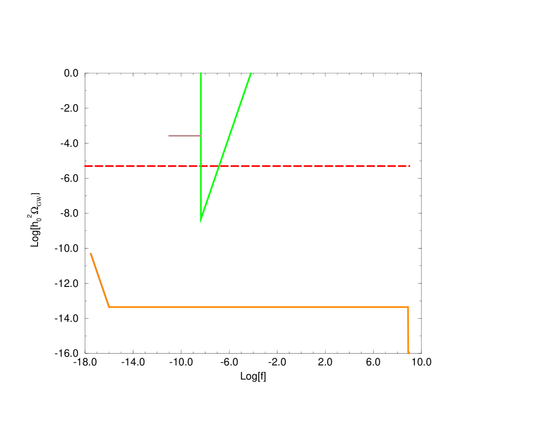
For $3\times 10^{-18}$ Hz $<f<f_{\rm eq}$ Hz, instead, we must compute the Bogoliubov coefficients for the RD-MD transition, and the total Bogoliubov transformation is obtained with the composition of the De Sitter-RD and RD-MD transformations. As always, the condition $f>3\times 10^{-18}$ Hz comes from requiring that the mode is inside the horizon today. Thus, these are the modes that were still outside the horizon at the RD-MD transition and re-entered the horizon before the present time.

A straightforward computation, similar to the one performed above, shows that in this frequency range the spectrum now goes like $1/f^{2}$ rather than being flat. So the final result is

$$h_{0}^{2}\Omega_{\rm gw}(f)\simeq 10^{-13}\left(\frac{f_{\rm eq}}{f}\right)^{2}\,\left(\frac{H}{10^{-4}M_{\rm Pl}}\right)^{2}\,,$$ (204)

if $3\times 10^{-18}\,{\rm Hz}<f<f_{\rm eq}\simeq 10^{-16}$ Hz, and

$$h_{0}^{2}\Omega_{\rm gw}(f)\simeq 10^{-13}\left(\frac{H}{10^{-4}M_{\rm Pl}}\right)^{2}\,,$$ (205)

for $f_{\rm eq}<f<f_{1}$. Finally, from the definition of $f_{1}$, eq. (198), we see that a mode that today has $f>f_{1}$, at the time of transition between De Sitter and RD had a wavelength smaller than the horizon; therefore these modes are never amplified, so that $f_{1}$ is the upper cutoff of the spectrum. The spectrum is shown in fig. 12.

Note that the behaviour $1/f^{2}$ in the region $3\times 10^{-18}$ Hz $<f<10^{-16}$ Hz is the same as the COBE bound, and is in fact due to the same physical reason, i.e. to the further amplification of modes that are inside the horizon at time of matter-radiation equilibrium. The comparison of eq. (204) with the COBE bound, eq. (139), then gives an upper limit on the Hubble constant during De Sitter inflation [235]; from a precise statistical analysis, the limit at 95% c.l. is [174]

$$H<6\times 10^{-5}M_{\rm Pl}\,.$$ (206)

9.2.2 Slow-roll inflation

In the above section we have considered a simplified model with an exact De Sitter inflation. If inflation is driven by a scalar field slowly rolling in a potential $V(\phi)$, the Hubble parameter during inflation is not exactly constant, and this results in a small tilt in the spectrum. Furthermore, scalar perturbations will also contribute to the COBE anisotropy, and the ratio of tensor to scalar perturbation is fixed by the choice of $V(\phi)$. Then, in the region $f_{\rm eq}<f<f_{1}$, one finds that $h_{0}^{2}\Omega_{\rm gw}(f)$ is not flat, as in eq. (205), but has a frequency dependence

$$h_{0}^{2}\Omega_{\rm gw}(f)\sim f^{n_{T}}\,,$$ (207)

where $n_{T}$ is called the spectral index for tensor perturbations. If $V_{*}$ is the value of the inflationary potential when the present horizon scale ($k=H_{0}$) crossed the horizon during inflation, and $V_{*}^{\prime}$ is the first derivative of the potential at that point, then, to lowest order in the deviation from scale invariance, and for single field models with a smooth potential [178, 249, 186]

$$n_{T}=-\frac{M_{\rm Pl}^{2}}{8\pi}\,\left(\frac{V_{*}^{\prime}}{V_{*}}\right)^{2}\,.$$ (208)

Therefore $n_{T}<0$, and the spectrum is decreasing rather than flat. Since the slow-roll condition is just $|\frac{M_{\rm Pl}^{2}}{8\pi}\,\left(\frac{V_{*}^{\prime}}{V_{*}}\right)^{2}|\ll 1$, then $|n_{T}|\ll 1$. It is convenient to define the scalar ($S$) and tensor ($T$) contributions to the quadrupole anisotropy [84],

$$S \equiv \frac{5\langle|a_{2m}^{S}|^{2}\rangle}{4\pi}=\frac{2.2(V_{*}/M_{\rm Pl}^{4})}{(M_{\rm Pl}V_{*}^{\prime}/V_{*})^{2}}\,,$$ (209)

$$T \equiv \frac{5\langle|a_{2m}^{T}|^{2}\rangle}{4\pi}=0.61(V_{*}/M_{\rm Pl}^{4})\,,$$ (210)

where the second equalities hold for slow-roll inflation. From eqs. (208), (209) and (210) it follows that

$$n_{T}=-\frac{1}{7}\,\frac{T}{S}\,.$$ (211)

To obtain the precise frequency dependence, we must also take into account the fact that the behaviours $h_{0}^{2}\Omega_{\rm gw}\sim 1/f^{2}$ and $h_{0}^{2}\Omega_{\rm gw}\sim$ const. in eqs. (204) and (205) hold only in the limits $f\ll f_{\rm eq}$ and $f\gg f_{\rm eq}$. Performing accurately the matching at $f=f_{\rm eq}$, taking into account the tilt $n_{T}$ and defining $k_{\rm eq}=2\pi f_{\rm eq}$, one finds the spectrum [249]

$$\frac{d\Omega_{\rm gw}}{d\log k}=\frac{\Omega_{0}^{2}(V_{*}/M_{\rm Pl}^{4})}{(k/H_{0})^{2-n_{T}}}\left[1+\frac{4}{3}\frac{k}{k_{\rm eq}}+\frac{5}{2}\left(\frac{k}{k_{\rm eq}}\right)^{2}\right]\,.$$ (212)

Defining $H_{*}^{2}=(8\pi/3)(V_{*}/M_{\rm Pl}^{2})$ and inserting the numerical values, we can rewrite it as

$$h_{0}^{2}\Omega_{\rm gw}(f) \simeq 0.8\times 10^{-13}\left(\frac{H_{*}}{10^{-4}M_{\rm Pl}}\right)^{2}\,\left(\frac{5\times 10^{-17}h_{0}\,{\rm Hz}}{f}\right)^{-n_{T}}\times$$ (213)

$$\left[1+\left(\frac{5\times 10^{-17}(h_{0}^{2}\Omega_{0})\,{\rm Hz}}{f}\right)+\left(\frac{6\times 10^{-17}(h_{0}^{2}\Omega_{0})\,{\rm Hz}}{f}\right)^{2}\right]\,.$$

The relation between $n_{T},T$ and $S$, eq. (211), goes in the wrong direction for the detection at interferometers: the higher the contribution of tensor perturbations at COBE, and therefore the maximum allowed value of the GW spectrum at, say, $f=10^{-16}$ Hz, the steeper is the decrease in the spectrum with the frequency. Furthermore, when extrapolating through a very large range of frequencies, one must also take into account that $n_{T}$ itself is not constant, but rather [172]

$$\frac{dn_{T}}{d\log k}=-n_{T}\frac{M_{\rm Pl}^{2}}{4\pi}\left(\frac{V_{*}^{\prime}}{V_{*}}\right)^{\prime}\,.$$ (214)

Combining these effects, one finds that, at a fixed frequency $f=10^{-4}$ Hz, relevant for LISA, the spectrum is maximized for $n_{T}\simeq-0.025$ [249], or $T/S\simeq 0.175$. Values of this order are realized in various models of inflation, although there are as well models that predict $T/S\sim 10^{-3}$. As discussed in sect. 7.2, GWs can contribute to the anisotropy only on angular scales larger than approximately $1^{o}$. Combining the results of COBE with other observations on smaller angular scales, one can place upper limits on $T/S$, and the analysis of ref. [195, 262] gives $T/S<0.5$, at 95% c.l.

Even with the value of $n_{T}$ that maximizes the signal at $f=10^{-4}$ Hz, the expected signal at LISA is of order $10^{-15}$, therefore various order of magnitudes below the expected sensitivity.

9.3 Pre-big-bang cosmology

9.3.1 The model

In recent years, a cosmological model derived from the low-energy effective action of string theory has been proposed [253, 130] (see ref. [179] for a recent review). The simplest starting point is the effective action in the metric-dilaton sector; at lowest order in the derivatives and in $e^{\phi}$ it is given by

$$S_{\rm eff}\sim\int d^{D}x\,\sqrt{-g}\,\left[e^{-\phi}\left(R+\partial_{\mu}\phi\partial^{\mu}\phi\right)\right]\,,$$ (215)

where $\phi$ is the dilaton field. This action receives two kinds of perturbative corrections: corrections parametrized by $e^{\phi}$, which are just higher loops in the field theory sense. And corrections proportional to $\alpha^{\prime}$, where $\lambda_{s}=\sqrt{2\alpha^{\prime}}$ is the string length, which are genuinely string effects, and take into account the finite size of the string. Since $\alpha^{\prime}$ has dimension of (length)², it is associated with higher derivative operators as for instance the square of the Riemann tensor, $R_{\mu\nu\rho\sigma}^{2}$. The remarkable fact observed in refs. [253, 130] is that there exits a regime in the early Universe evolution of this model, where the perturbative approach is well justified, and in a first approximation one can use eq. (215), neglecting the corrections. This regime occurs if we take as initial condition a Universe at weak coupling and low curvatures. Then, a generic inhomogeneous string vacuum shows a gravitational instability [62]. Specializing for simplicity to a homogeneous model, the solution of the equations of motion derived from the action (215) reads, for generic anisotropic FRW scale factors $a_{i}(t)$, $i=1,\ldots D-1$,

$$a_{i}(t) = (-t)^{c_{i}}\,,$$

$$\phi_{i}(t) = \phi_{0}+c_{0}\log(-t)\,,$$ (216)

with

$$\sum_{i=1}^{D-1}c_{i}^{2}=1\,,\hskip 28.45274pt\sum_{i=1}^{D-1}c_{i}=1+c_{0}\,.$$ (217)

This is just a generalization in the presence of the dilaton of the Kasner solution of general relativity. Considering for simplicity an isotropic model, one has in particular a solution with $c_{i}=-1/\sqrt{D-1}$, $c_{0}=-1-\sqrt{D-1}$. This corresponds to a superinflationary evolution: the Hubble parameter $H=\dot{a}/a$ grows until it reaches the string scale $\sim 1/\lambda_{s}$, and finally formally diverges at a singularity. When $H\sim 1/\lambda_{s}$, of course, the description based on the lowest order action is not anymore adequate. Much work has been devoted recently to understanding how string theory cures the apparent singularity, and if it is possible to match this ‘pre-big-bang’ phase to standard post-big-bang cosmology [60, 61, 160, 101, 88, 128, 187, 114, 59, 115]. Apart from the phenomenological aspects concerning GWs that we will discuss, it is clear that the problem has great conceptual interest, since it a theoretically well motivated attempt to cure the Big-Bang singularity.

One can then investigate whether pertubative corrections succeed in turning the regime of pre-big-bang accelerated expansion into the standard decelerated expansion. Indeed, the inclusion of $\alpha^{\prime}$ corrections can turn the unbounded growth of the curvature into a De Sitter phase with linearly growing dilaton [128]. Since in this new regime the dilaton keeps growing linearly, finally also $e^{\phi}$ gets large, even if the evolution started at very weak coupling; at this stage loop corrections are important, and they can trigger the exit from the De Sitter phase [59, 115]. An example of this behaviour, using loop corrections derived from orbifold compactifications of string theory, has been found in ref. [115], and is shown in fig. 13.

Figure 13: The evolution of the Hubble parameter $H$ and of $\dot{\phi}$ in string cosmology with $\alpha^{\prime}$ and loop corrections (from ref. [115]).

These results are encouraging, but various technical limitations in the analysis have also indicated that most probably the true resolution of the singularity problem lies outside the domain of validity of the perturbative approach [115]. In this case one must take into account that at strong coupling and large curvature new light states appear and then the approach based on the effective supergravity action plus string corrections breaks down. The light modes are now different and one must turn to a new effective action, written in terms of the new relevant degrees of freedom. In particular, at strong coupling $D$-branes [210] are expected to play an important role, since their mass scales like the inverse of the string coupling, $\sim 1/g$ and they are copiously produced by gravitational fields [190].

For the purpose of computing the amplification of vacuum fluctuations in this model, the approach that can be taken is to consider a model with three phases: first an isotropic superinflationary evolution described by eq. (216), with the value of the constants $c_{i},c_{0}$ determined by eq. (217). Then this phase is matched to a De Sitter phase with linearly growing dilaton, which may be considered as representative of a typical solution in the large curvature regime; the constant values of $H,\dot{\phi}$ in this phase are taken as free parameters, of the order of the string scale. Finally, we match this phase to the standard RD era. Of course, this model can only be taken as indicative of possible behaviours in string cosmology, since what happens in the large curvature phase is certainly much more complicated. However, we will see that some important characteristics of the GW spectrum depend only on the low curvature regime, where we can use the lowest order effective action and therefore is under good theoretical control.

Variants of this model can of course be constructed. In particular, ref. [197] considers the effect of a second burst of inflation, or of the possibility that the Universe becomes temporarily dominated by long-lived massive particles, as for instance the moduli fields of string theory, which then decay, restoring a standard RD phase [137].

9.3.2 Production of GWs

We can now discuss the production of GWs through amplification of vacuum fluctuations in this model [131, 126, 56] (see also refs. [63, 57, 55, 10, 188, 191, 123, 124, 125, 86, 152]). We specialize for illustration to a isotropic model compactified to four dimensions. Writing the scale factors and the dilaton in terms of conformal time, from eq. (216), we find that for $-\infty<\eta<\eta_{s}$ (with $\eta_{s}<0$), we have a dilaton-dominated regime with

$$a(\eta) = -\frac{1}{H_{s}\eta_{s}}\left(\frac{\eta-(1-\alpha)\eta_{s}}{\alpha\eta_{s}}\right)^{-\alpha}$$ (218)

$$\phi(\eta) = \phi_{s}-\gamma\log\frac{\eta-(1-\alpha)\eta_{s}}{\eta_{s}}\,.$$ (219)

and the Kasner conditions eq. (217) give $\alpha=1/(1+\sqrt{3}),\gamma=\sqrt{3}$.

At a value $\eta=\eta_{s}$ the curvature becomes of the order of the string scale, and we assume a De Sitter expansion with linearly growing dilaton; in terms of conformal time, this means

$$a(\eta)=-\frac{1}{H_{s}\eta}\,,\hskip 22.76219pt\phi(\eta)=\phi_{s}-2\beta\log\frac{\eta}{\eta_{s}}\,.$$ (220)

The parameter $H_{s}$ is of the order of the string scale, while $\beta$ is a free parameter of the model. Note that $2\beta=\dot{\phi}/H_{s}$, where $\dot{\phi}$ is the derivative with respect to cosmic time.

The stringy phase lasts for $\eta_{s}<\eta<\eta_{1}$ (again $\eta_{1}<0$), and at $\eta_{1}$ we match this phase to a standard RD era. This gives, for $\eta_{1}<\eta<\eta_{r}$, (with $\eta_{r}>0$)

$$a(\eta)=\frac{1}{H_{s}\eta_{1}^{2}}\,(\eta-2\eta_{1})\,,\hskip 22.76219pt\phi=\phi_{0}\,.$$ (221)

After that, the standard matter dominated era takes place. We have chosen the additive and multiplicative constants in $a(\eta)$ in such a way that $a(\eta)$ and $da/d\eta$ (and therefore also $da/dt$) are continuous across the transitions.

The equation for the Fourier modes of metric tensor perturbations for the two physical polarizations in the transverse traceless gauge is [126]

$$\frac{d^{2}\psi_{k}}{d\eta^{2}}+\left[k^{2}-V(\eta)\right]\psi_{k}=0\,,$$ (222)

$$V(\eta)=\frac{1}{a}\,e^{\phi/2}\,\frac{d^{2}}{d\eta^{2}}\left(a\,e^{-\phi/2}\right)\,.$$ (223)

Note that, for constant $\phi$, $V(\eta)$ reduces to eq. (176). Inserting the expressions (218-221), the potential is

$$V(\eta)=\frac{1}{4}\,(4\nu^{2}-1)\left(\eta-(1-\alpha)\eta_{s}\right)^{-2},\hskip 28.45274pt-\infty<\eta<\eta_{s}$$

$$V(\eta)=\frac{1}{4}\,(4\mu^{2}-1)\eta^{-2},\hskip 113.81102pt\eta_{s}<\eta<\eta_{1}$$ (224)

$$V(\eta)=0\,,\hskip 182.09763pt\eta_{1}<\eta<\eta_{r}$$

where $2\mu=|2\beta-3|,2\nu=|2\alpha-\gamma+1|$. From $\alpha=1/(1+\sqrt{3})$ and $\gamma=\sqrt{3}$, we get $\nu=0$. The exact solutions of eq. (222) in the three regions are

$$\psi_{k}(\eta)=\sqrt{|\eta-(1-\alpha)\eta_{s}|}\,C\,H_{0}^{(2)}(k|\eta-(1-\alpha)\eta_{s}|)\,,\hskip 5.69054pt-\infty<\eta<\eta_{s}$$

$$\psi_{k}(\eta)=\sqrt{|\eta|}\,\left[A_{+}\,H_{\mu}^{(2)}(k|\eta|)+A_{-}\,H_{\mu}^{(1)}(k|\eta|)\right]\,,\hskip 36.98857pt\eta_{s}<\eta<\eta_{1}$$ (225)

$$\psi_{k}(\eta)=i\,\sqrt{\frac{2}{\pi k}}\,\left[B_{+}\,e^{ik\eta}-B_{-}\,e^{-ik\eta}\right]\,,\hskip 85.35826pt\eta_{1}<\eta<\eta_{r}$$

where $H_{\nu}^{(1,2)}$ are Hankel’s functions. As we have seen in sect. 9.2.1, it is convenient to trade $\eta_{s},\eta_{1}$ for more physically meaningful quantities. As before, we then write

$$k|\eta_{1}|=2\pi fa(t_{0})|\eta_{1}|=\frac{2\pi f}{H_{s}}\,\frac{a(t_{0})}{a(t_{1})}=\frac{2\pi f}{H_{s}}\left(\frac{t_{0}}{t_{\rm eq}}\right)^{2/3}\left(\frac{t_{\rm eq}}{t_{1}}\right)^{1/2}\,,$$ (226)

and therefore the parameter $\eta_{1}$ can be traded for a parameter $f_{1}$ defined by

$$k|\eta_{1}|=\frac{f}{f_{1}}\,,\hskip 28.45274ptf_{1}\simeq 4.3\cdot 10^{10}{\rm Hz}\,\,\left(\frac{H_{s}}{0.15\,M_{\rm pl}}\right)\,\left(\frac{t_{1}}{\lambda_{s}}\right)^{1/2}\,.$$ (227)

where we have chosen a reference value $H_{s}$ of the order of the string scale, and $t_{1}\simeq\lambda_{s}$. Similarly we can introduce a parameter $f_{s}$ instead of $\eta_{s}$, from $k|\eta_{s}|={f}/{f_{s}}$. This parameter depends on the duration of the string phase, and therefore, contrarily to $f_{1}$, is totally unknown, even as an order of magnitude. However, since $|\eta_{1}|<|\eta_{s}|$, we have $f_{s}<f_{1}$.

To summarize, the model has a parameter $f_{s}$ with dimensions of a frequency, which can have any value in the range $0<f_{s}<f_{1}$, with $f_{1}\sim 1-100$ GHz, and a dimensionless parameter $\mu\geq 0$ (or equivalently $\beta$ with $2\mu=|2\beta-3|$).

Performing the matching between the three phases one finally gets the spectrum. The exact form is [63]

$$\Omega_{\rm gw}(f)=a(\mu)\,\frac{(2\pi f_{s})^{4}}{H_{0}^{2}M_{\rm pl}^{2}}\,\left(\frac{f_{1}}{f_{s}}\right)^{2\mu+1}\,\left(\frac{f}{f_{s}}\right)^{5-2\mu}\,\left|H_{0}^{(2)}\left(\frac{\alpha f}{f_{s}}\right)\,J_{\mu}^{\prime}\left(\frac{f}{f_{s}}\right)\right.+$$

$$\left.+H_{1}^{(2)}\left(\frac{\alpha f}{f_{s}}\right)\,J_{\mu}\left(\frac{f}{f_{s}}\right)-\frac{(1-\alpha)}{2\alpha}\,\frac{f_{s}}{f}\,H_{0}^{(2)}\left(\frac{\alpha f}{f_{s}}\right)\,J_{\mu}\left(\frac{f}{f_{s}}\right)\right|^{2}\,,$$ (228)

where $a(\mu)$ is a number, which depends on $\mu$. Expanding this expression for small values of $f/f_{s}$ one gets a result of the form

$$\Omega_{\rm gw}(f)\sim\frac{(2\pi f_{s})^{4}}{H_{0}^{2}M_{\rm pl}^{2}}\left(\frac{f_{1}}{f_{s}}\right)^{2\mu+1}\left(\frac{f}{f_{s}}\right)^{3}\left\{a_{1}+\left[\left(a_{2}\log\frac{\alpha f}{2f_{s}}+a_{3}\right)\right]^{2}\right\}\,,$$ (229)

where $a_{1},a_{2},a_{3}$ depend on $\mu$.

Figure 14: The spectrum of GWs due to amplification of vacuum fluctuations in string cosmology, compared with the COBE bound (dot-dashed), pulsar bound (asterisk) and nucleosynthesis (dotted), for a choice of the parameters $f_{s}=10$ Hz, $\mu=1.5$ (from ref. [63]).

Figure 15: The GW spectrum, enlarging the region between the Hz and the kHz, for $f_{s}=100$ Hz, $\mu=1.4$. The dashed and dot-dashed lines are the low- and high-frequency limits (from ref. [63]).

In the opposite limit $f\gg f_{s}$ (but still $f$ smaller than the cutoff $f_{1}$), one has instead

$$\Omega_{\rm gw}(f)\sim\frac{(2\pi f_{s})^{4}}{H_{0}^{2}M_{\rm pl}^{2}}\,\left(\frac{f_{1}}{f_{s}}\right)^{2\mu+1}\,\left(\frac{f}{f_{s}}\right)^{3-2\mu}=\frac{(2\pi f_{1})^{4}}{H_{0}^{2}M_{\rm pl}^{2}}\,\left(\frac{f}{f_{1}}\right)^{3-2\mu}\,.$$ (230)

Both limits reproduces the frequency dependence first found in ref. [126, 56]. It is important to stress that in the high frequency limit the unknown parameter $f_{s}$ cancels.

This spectrum has quite interesting properties, depending on the two free parameters $f_{s}$ and $\mu$. First of all, it goes like $f^{3}$ at low frequencies. This result is a consequence of the behaviour of the cosmological model in the superinflationary pre-big-bang phase, where everything is under good theoretical control, so this is a rather general prediction of the model. This means that $h_{0}^{2}\Omega_{\rm gw}(f)$ can evade the COBE bound very easily, and yet be large in the range accessible to interferometers. This is very different from slow-roll inflation, where instead the spectrum is decreasing.

If however the spectrum would behave as $f^{3}$ for all frequencies, up to the cutoff $f_{1}$, it would be totally neglegible at, say, 1 kHz, since the value of $h_{0}^{2}\Omega_{\rm gw}(f)$ at the cutoff frequency $f_{1}$ is bounded by the nucleosynthesis limit discussed in sect. 7.1. However, above the unknown frequency $f_{s}$, the spectrum predicted by this model changes and behaves as $f^{3-2\mu}$; this reflects the fact that the Universe changed regime and entered a phase of De Sitter inflation with linearly growing dilaton. The parameter $\mu$ measures the growth of the dilaton in units of the Hubble constant $H_{s}$ during the string phase, and for an almost constant dilaton, $3-2\mu\simeq 0$.

This means that, in some range for the parameters $f_{s}$ and $\mu$, it is possible to have the optimal situation from the point of view of interferometers: a spectrum that grows at very low frequencies, so that it can evade the COBE bound, and then flattens, at the maximum level allowed by the nucleosynthesis limit.

The resulting spectrum is shown in fig. 14, compared to the COBE, pulsar and nucleosynthesis bounds discussed in sect. 11. Fig. 15 enlarges the frequency range relevant for ground-based interferometers, displaying some features of the spectrum which might be a signature of this background.

Finally, it is clear that in this model GWs cannot be responsible for the COBE anisotropies, since the $\sim f^{3}$ behaviour makes $h_{0}^{2}\Omega_{\rm gw}$ neglegible at very low frequencies. In the pre-big-bang model, a possible seed for the CMBR anisotropies can be provided by pseudo-scalar fields [85, 87, 100, 64, 58, 196].

10 Other production mechanisms

10.1 Phase transitions

In the history of the Universe are expected a number of phase transition. In particular, the QCD phase transition takes place at $T_{*}\sim 150$ MeV. Above this temperature quarks and gluons are deconfined and form a quark-gluon plasma, while below they are in the confined phase. Recent lattice calculations with three quark flavors and with the physical mass for the strange quark, using Wilson fermions, suggest that the phase transition is first order [155], but the issue is not yet settled (see also [229] for a detailed discussion of cosmological consequencies of the QCD phase transition). Around $T_{*}\sim 100$ GeV we expect the electroweak phase transition, when $SU(2)\times U(1)$ breaks to $U(1)_{\rm em}$. Further phase transitions could occur even earlier, at the grand unified scale. These phase transitions are dramatic events in the history of the Universe, and are good places to look for GW production.

Furthermore, phase transition will in general modify previously produced spectra [234]. This follows from the fact that during the phase transition one can have a large drop in the number $g_{S}$ of effective species (e.g. by a factor $\sim 3$ during the QCD phase transition). Since the entropy $S\sim g_{S}a^{3}T^{3}$ is constant, this results in a smaller value of the growth rate of $H^{-1}$ and therefore in a different rate at which modes cross into the horizon. For the QCD transition this results in a step in the spectrum at a frequency $f\sim 10^{-7}$ Hz (determined by the value of the Hubble parmeter at the transition), so that the spectrum above $10^{-7}$ Hz is diminuished by approximately 30% [234]. Similar drops happen at $e^{+}e^{-}$ annihilation, with a step at $f\sim 10^{-10}$ Hz, and at the GUT phase transition, with a step in the GHz region.

10.1.1 Bubble collisions

In first order phase transitions the Universe finds itself in a metastable state. True vacuum bubbles are then nucleated via quantum tunneling. In strongly first order phase transition the subsequent bubble dynamics is relatively simple: once the bubble are nucleated, if they are smaller than a critical size their volume energy cannot overcome the shrinking effect of the surface tension, and they disappear. However, as the temperature drops below the critical temperature $T_{c}$, it becomes possible to nucleate bubble that are larger than this critical size. These ‘critical bubbles’ start expanding, until their wall move at a speed close to the speed of light. The energy gained in the transition from the metastable state to the ground state is transferred to the kinetic energy of the bubble wall. As the bubble expands, more and more regions of space convert to the ground state, and the wall becomes more and more energetic. At the same time, it also becomes thinner, and therefore the energy density stored in the wall increases very fast. As long as we have a single spherical bubble, this large energy of course cannot be converted in GWs. But when two bubbles collide we have the condition for the liberation of a large amount of energy into GWs. In particular, there are two possible ‘combustion’ modes for the two bubbles: detonation [237], that basically takes place when the boundaries propagate faster than the speed of sound, and deflagration, when instead they move slower. In the first case there is a large production of GWs [148, 260, 170].

The characteristic frequency, as seen today, of these GWs is given by eq. (157), with $T_{*}$ equal to the temperature of the phase transition. First of all, we must estimate the parameter $\epsilon$ that enters eq. (157). Plausible values of $\epsilon$ have been discussed in detail by Hogan [148] and by Witten (ref. [260], app. B). In the case of the QCD and electroweak transitions $\epsilon\sim 1$ is excluded because otherwise in the bubble collisions there would be overproduction of primordial black holes. Production of primordial black holes is severely constrained because the energy density of primordial black holes scales like $1/a^{3}$ in the RD phase, and therefore they would come to dominate the energy density of the Universe. In particular, the Universe would not be radiation dominated during nucleosynthesis. Actually, primordial black holes can evaporate through emission of Hawking radiation. However, in order to evaporate before nucleosynthesis, the scale at which the phase transition takes place must be higher than $10^{11}$ GeV [252]. Therefore $\epsilon$ could be of order one in phase transitions which take place at these temperatures, but not in the QCD or electroweak phase transition.

To estimate $\epsilon$ it is necessary to make assumptions about how the phase transition is nucleated. If it is nucleated by thermal fluctuations, ref. [148] suggests an upper bound $\epsilon\raise 1.72218pt\hbox{$<$}\kern-8.00003pt\lower 2.6694pt\hbox{$\sim$}10^{-2}$, but recent lattice simulations (restricted however to pure QCD without fermions) give a much smaller value $\epsilon\sim 10^{-6}$, which would make the GWs from the QCD transition neglegible, as will be clear below. For nucleation of bubbles via quantum tunneling a detailed analysis has been done in ref. [250]. The relevant parameter is the nucleation rate; the phase transition can be modelled assuming an exponential bubble nucleation rate per unit volume,

$$\Gamma=\Gamma_{0}e^{\beta t}\,.$$ (231)

The parameter $\beta$ sets the scale for the typical time variation, and therefore the frequency at time of production, $f_{*}$, is determined by $\beta$. In fact, ref. [170] founds that the spectrum peaks at $2\pi f_{*}\simeq 2\beta$. Then

$$\frac{1}{\epsilon}\equiv\frac{f_{*}}{H_{*}}\simeq\frac{\beta}{\pi H_{*}}\,.$$ (232)

Of course, $\beta$ is a model-dependent quantity, but for a wide class of models one typically finds $\epsilon\sim 10^{-3}-10^{-2}$ [147, 148, 250, 171, 170].

If however the transition is nucleated by impurities (which is most often the case, except in very pure and homogeneous samples) the issue is much more complicated. For instance, the impurities could be given by turbolent motion of the cosmic fluid generated prior to the QCD epoch; they would depend on the detailed spectrum of the fluid motion, or in general on the characteristic distance between impurities, and in this case $\epsilon$ is basically impossible to estimate, even as an order of magnitude [260].

Coming back to the simplest case of nucleation by quantum or thermal fluctuations, for the electroweak phase transition, ref. [170] finds

$$\frac{\beta}{H_{*}}\simeq 1.3\times 10^{-3}$$ (233)

and therefore

$$f_{0}\simeq 4.1\times 10^{-3}\,{\rm Hz}\,.$$ (234)

This phase transition is therefore very relevant for LISA. With the same value for $\epsilon$, the QCD phase transition would instead peak around $f_{0}\sim 4\times 10^{-6}$ Hz. A smaller value of $\epsilon$ is required to bring it into the frequency window of LISA.

A first estimate of the value of $h_{0}^{2}\Omega_{\rm gw}$, that as we will see really holds only for strongly first order phase transitions, can be given as follows [252]. The typical wavelength $\lambda_{*}$ produced in the collision of two bubbles will be of the order of the radius of the bubbles when they collide, which in turn is a fraction of the horizon scale $H_{*}^{-1}$. The energy liberated in GWs in the collision of two bubbles is of order

$$E_{GW}\sim\frac{GM_{B}^{2}}{\lambda_{*}}\,,$$ (235)

where $M_{B}\sim\rho_{\rm vac}\lambda_{*}^{3}$ is the energy of a typical bubble and $\rho_{\rm vac}$ the difference in energy density from the metastable state to the ground state. The fraction of the false vacuum energy that goes into GWs instead of going into $\rho_{\gamma}$ is therefore $E_{\rm GW}/M_{B}$. Since

$$\frac{E_{\rm GW}}{M_{B}}\sim\frac{GM_{B}}{\lambda_{*}}\sim G\rho_{\rm vac}\lambda_{*}^{2}$$ (236)

and $H_{*}^{2}\sim G\rho_{\rm vac}$, we get, at time of production

$$\rho_{\rm gw}\sim\lambda_{*}^{2}H_{*}^{2}\rho_{\gamma}=\epsilon^{2}\rho_{\gamma}\,.$$ (237)

Therefore $\rho_{\rm gw}$ is related to $\rho_{\gamma}$, and the basic reason is that there is essentially only one dimensionful parameter that enters in the estimate. If we neglect the variation in $g(T)$ from time of production to the present value, $\rho_{\rm gw}/\rho_{\rm\gamma}$ is almost constant, and since today $h_{0}^{2}\rho_{\rm\gamma}/\rho_{c}\simeq 2.5\times 10^{-5}$, this quick order of magnitude estimate gives $h_{0}^{2}\Omega_{\rm gw}(f_{0})\sim 10^{-5}\epsilon^{2}$. However, further suppression factors appears in the accurate computation of ref. [170], which gives

$$h_{0}^{2}\Omega_{\rm gw}(f_{0})\simeq 1.1\times 10^{-6}\kappa^{2}\left(\frac{H_{*}}{\beta}\right)^{2}\left(\frac{\alpha}{1+\alpha}\right)^{2}\left(\frac{v^{3}}{0.24+v^{3}}\right)\left(\frac{100}{g_{*}}\right)^{1/3}\,.$$ (238)

Here $\alpha$ is the ratio of vacuum energy to thermal energy in the symmetric phase. It characterizes the strength of the phase transition; for $\alpha\rightarrow 0$ we have a very weak first order and for $\alpha\rightarrow\infty$ a very strong first order phase transition. For the electroweak phase transition, ref. [170] gives

$$\alpha=1.4\times 10^{-3}\,.$$ (239)

$\kappa$ is an efficiency factor quantifying the fraction of vacuum energy which goes into bubble wall kinetic energy, and in the electroweak case is estimated to be $\kappa\simeq 7.8\times 10^{-3}$. Finally, $v$ is the velocity of the bubble wall, and is approximately equal to the speed of sound during RD, $v\simeq 1/\sqrt{3}$. Altogether, these suppression factors give a disappointing

$$h_{0}^{2}\Omega_{\rm gw}\sim 10^{-22}\,.$$ (240)

These suppression factors are a consequence of the fact that the electroweak phase transition is very weakly first order, if first order at all. It is clear that strongly first order phase transitions are needed for a detectable signal.

Quite interestingly, the requirement of strongly first order phase transition is the same that it is necessary to make possible electroweak baryogenesis (see e.g. ref. [220] for a recent review). In particular, the ways in which baryons can be produced have been separated into ‘local baryogenesis’, when both baryon number violating and CP violating processes occur near the bubble wall, and ‘nonlocal baryogenesis’, when only CP violating processes take place near the wall. The condition for local baryogenesis to dominate is that the speed of the wall be greater than the speed of sound, which is the same condition for detonation to dominate the bubble-bubble collisions.

Partly motivated by the importance for baryogenesis, there have been many recent investigations on the strength of the phase transition in extensions of the Standard Model, and in particular in the Minimal Supersymmetric Standard Model (MSSM) [134, 203, 103, 52]. Both analytical [68, 97, 102, 50, 183, 107, 96] and lattice [175, 176, 75] computations have shown that in the MSSM the phase transition can be strongly first order if the top squark is lighter then the top quark. The observation of a relic stochastic background at LISA could therefore give us a hint for physics beyond the Standard Model.

10.1.2 Turbolence

For weakly first order phase transitions the situation is actually more complex. Bubble nucleation occurs both via quantum tunneling and with thermal fluctuations, and the subsequent evolution of the bubble depends on the interaction of the wall with the surrounding plasma; part of the energy gained in the transition from the metastable state to the ground state is used to heat up the plasma, and another fraction is converted into bulk motion of the fluid. If the Reynolds number of the Universe at the phase transition is large enough, then this results in the onset of turbolence in the plasma, and this is another powerful source of GWs.

The estimates for the characteristic frequency and for $h_{0}^{2}\Omega_{\rm gw}$ turn out to be [170]

$$f_{0}\simeq 2.6\times 10^{-8}\,{\rm Hz}\,\frac{v_{0}}{v}\left(\frac{\beta}{H_{*}}\right)\left(\frac{T_{*}}{1\,{\rm GeV}}\right)\left(\frac{g_{*}}{100}\right)^{1/6}\,,$$ (241)

$$h_{0}^{2}\Omega_{\rm gw}\simeq 10^{-5}\left(\frac{H_{*}}{\beta}\right)^{2}vv_{0}^{6}\left(\frac{100}{g_{*}}\right)^{1/3}\,,$$ (242)

where $v_{0}$ is the fluid velocity on the largest length scales on which the turbolence is being driven, and $v$ the velocity of the bubble wall. These estimates indicate that fully developed turbolence can be comparable, or even more potent than bubble collisions in generating GWs.

10.1.3 Scalar field relaxation

Consider a global phase transition in the early Universe, associated with some scalar field $\phi$ that, below a critical temperature, gets a vacuum expectation value $\langle\phi\rangle$. For causality reasons, in an expanding Universe the scalar field cannot have a correlation length larger than the horizon size. So, even if the configuration which minimizes the energy is a constant field, the field will be constant only over a horizon distance. During the RD phase the horizon expands, and the field will relax to a spatially uniform configuration within the new horizon distance. This relaxation process will in general produce gravitational waves, since there is no reason to expect $\langle T_{\mu\nu}\rangle$ for the classical field just entering the horizon to be spherically symmetric [173]. A simple estimate of the spectrum produced makes use of the fact that the characteristic scale of spatial or temporal variation of the field is given by the inverse of the Hubble constant, $H^{-1}$, at the value of time under consideration. Then, the energy density of the field is $\rho\sim(\partial\phi)^{2}\sim\langle\phi\rangle^{2}H^{2}$. The total energy in a Hubble volume is $\rho H^{-3}\sim\langle\phi\rangle^{2}H^{-1}$ and the corresponding quadrupole moment is $Q\sim(\rho H^{-3})H^{-2}\sim\langle\phi\rangle^{2}H^{-3}$, times a constant smaller than one, which measures the non-sphericity of the configuration. The energy liberated in GWs in a horizon time is then given by [173]

$$\Delta E\sim H^{-1}\times{\rm Luminosity}\sim H^{-1}G\left(\frac{d^{3}Q}{dt^{3}}\right)^{2}\sim G\langle\phi\rangle^{4}H^{-1}\,,$$ (243)

and the energy density of GW produced is

$$\left(\frac{d\rho_{\rm gw}}{d\log f}\right)_{*}\sim\frac{\Delta E}{H^{-3}}\sim G\langle\phi\rangle^{4}H^{2}\,.$$ (244)

This is the energy density at a frequency $f\sim H$, at a value of time $t=t_{*}(f)$ which is the time when the mode with frequency $f$ enters the horizon. The asterisk in $(d\rho/d\log f)_{*}$ reminds that this quantity is evaluated at horizon crossing, therefore at different values of time for different frequencies. However, in the RD phase, the energy density scales like $\rho\sim 1/a^{4}(t)\sim t^{-2}$ and $H\sim t^{-1}$ so that $\rho$ scales as $H^{2}$. Therefore, eq. (244) means that, if we evaluate $d\rho/d\log f$ at the same value of time, for all frequencies which at this value of time are inside the horizon, the spectrum is flat, $h_{0}^{2}\Omega_{\rm gw}(f)\sim$ const. This is a rather nice example of how a flat spectrum can follow simply from the requirement of causality and simple dimensional estimates. The simplest way to redshift eq. (244) to the present time is to use $H^{2}=(8\pi/3)G\rho_{\gamma}$, so that eq. (244) can be written as

$$\left(\frac{d\rho_{\rm gw}}{d\log f}\right)_{*}\sim\frac{8\pi}{3}G^{2}\langle\phi\rangle^{4}(\rho_{\gamma})_{*}\,,$$ (245)

where both sides are evaluated at horizon crossing. Then $\rho_{\rm gw}$ redshifts as $1/a^{4}$, $\rho_{\gamma}$ adiabatically, eq. (153), and $\rho_{\rm rad}=g(T)\rho_{\gamma}$, so that $(\Omega_{\rm gw})_{0}=(g_{0}/g_{*})^{1/3}(\Omega_{\rm gw})_{*}$, and therefore eq. (244) gives, for the energy density today,

$$h_{0}^{2}\Omega_{\rm gw}\sim 5\times 10^{-5}\left(\frac{\langle\phi\rangle}{M_{\rm Pl}}\right)^{4}\left(\frac{100}{g_{*}}\right)^{1/3}\,.$$ (246)

A quite similar mechanism has been studied in ref. [149], considering a theory with a multicomponent scalar field $\vec{\phi}$ and an effective potential $V(\vec{\phi})$ with degenerate minima at a set of points with $|\vec{\phi}|=\phi_{0}\gg 1$. The direction in field space with $\partial V/\partial\vec{\phi}$ define massless Goldstone bosons. Cooling down from a state with higher symmetry generates spatial gradients in $\vec{\phi}$ and therefore excites these Goldstone bosons. The modes that enter the horizon then produce GWs with the same mechanism described above, and again one finds eq. (246).

Clearly, the effect is significant only if $\langle\phi\rangle$ is not too far from the Planck mass. Since the mechanism is completely general, it is well conceivable that it might take place in string theory, which has a multitude of scalar fields, like the dilaton and the moduli of the compactification. At tree level these fields correspond to flat directions, but non-perturbative effects will lift the degeneracy; it is then very natural to expect that at the same time they produce a number of degenerate or almost degenerate vacua. In this case this effect could give an extremely interesting signal both for LISA and for ground based interferometers.

Of course, if we want to avoid the COBE bound, it is necessary to suppress the spectrum at low frequencies. As suggested in ref. [149], this might happen if the Goldstone modes are coupled to fields that strongly damp their oscillations after a certain epoch. For example there could be a second phase transition that removes the degeneracy between the minima of the potential; the field would then relax everywhere to a single minimum, suppressing further GW production.

Finally, another related production mechanism is the collapse of solitons or of unstable domain walls [135, 136]. In this case the spectrum is quite peaked, at a frequency determined by the expectation value of the scalar field $\phi_{0}$, and for $\phi_{0}$ of the order of the electroweak scale the signal would be relevant for LISA.

10.2 Cosmic strings

Cosmic strings are topological defect that might have formed during phase transitions in the early Universe (see e.g. [254, 255] and references therein). Interest in cosmic strings has also been fueled by the fact that they were considered a candidate for seeding structure formations. The most recent comparison with CMB anisotropies show that in models with vanishing cosmological constant they do not reproduce the dependence of the anisotropy from the multipole moment [214, 6]. However, with a non-vanishing cosmological constant they can still be a viable option [28, 34].

The spectrum of GWs produced by cosmic strings is discussed in detail in refs. [254, 255, 66, 8, 67, 33]. Gravitational waves are produced by the relativistic oscillations of a cosmic string, in a cosmic string network. The dynamics of this string network has been studied in detail, and it has been found that it obeys a scaling property, so that the only relevant scale is given by the Hubble length. Small loops oscillate producing GWs and disappear, while more small loops are chooped of very long strings, replacing the loops that disappear, and the network has a self-similar configuration, with loops of all lengthscales. Since the wavelength of the GWs emitted is fixed by the length of the loop, the spectrum of the cosmic string network extends across a very large frequency band.

The spectrum has two main features: an almost flat region that extends from $f\sim 10^{-8}$ Hz up to $f\sim 10^{10}$ Hz, and a peak in the region $f\sim 10^{-12}$ Hz.

At LIGO/VIRGO frequencies we are in the flat part of the spectrum, and the typical estimate of the intensity is of order

$$h_{0}^{2}\Omega_{\rm gw}\sim 10^{-8}-10^{-7}\,.$$ (247)

(Similar results are obtained from hybrid topological defects [192]). The scale for these numbers is given first of all by the combination $(G\mu)^{2}$, where $\mu$ is the mass per unit length of the string. It comes from the fact that a loop radiates with a power $P\sim\gamma G\mu^{2}$, ($\gamma$ is a dimensionless constant) while, evaluating $h_{0}^{2}\Omega_{\rm gw}$, another factor of $G$ comes from $1/\rho_{c}$. For strings created at the GUT scale $G\mu\sim 10^{-6}$. Then, there are also large numbers related to the number of strings per horizon volume, which is thought to be of order 50, to the fact that also $\gamma\sim 50$, and to the size of the loops at formation time [8], that finally give a value $h_{0}^{2}\Omega_{\rm gw}\sim 10^{-8}-10^{-7}$.

For the cosmic string spectrum the most relevant bound comes from the pulsars, discussed in sect. 11. Pulsar timing implies a bound on the mass per unit length of the string [33]

$$\frac{G\mu}{c^{2}}<(5.4\pm 1.1)\times 10^{-6}\,.$$ (248)

For comparison, the value of $\mu$ obtained fitting CMBR anisotropies in an open Universe is $(G\mu)/c^{2}\sim 1.7\times 10^{-6}$ for $\Omega_{0}=0.2$ [27]. The improvement in pulsar timing expected in the next few years, see sect. 11, will therefore be crucial for testing the cosmic string scenario.

10.3 Production during reheating

If we have an inflationary phase below the Planck scale, there is no gravitational analog of the 2.7K radiation. At the Planck scale photons and gravitons can be produced simply by thermal collisions, with probably similar production rates. However, the particles produced in this way at the Planck (or string) scale are exponentially diluted by the subsequent inflationary phase, and the photons that we see today in the cosmic microwave background radiation (CMBR) have been produced during the reheating era which terminated the inflationary phase.

Since the reheating temperature $T_{\rm rh}<M_{\rm infl}\ll M_{\rm Pl}$, thermal collisions are by now unable to produce a substantial amount of gravitons. However, in this case relic GWs can be produced through some non-equilibrium phenomenon connected with the reheating process. For a process that takes place at the reheating temperature $T_{\rm rh}$ the estimate of the characteristic frequency is given by eq. (157) with $T_{*}=T_{\rm rh}$. In principle the reheating temperature can be between a minimum value at the TeV scale (since this is the last chance for baryogenesis, via the anomaly in the electroweak theory) and a maximum value $T_{\rm rh}\sim M_{\rm infl}\raise 1.72218pt\hbox{$<$}\kern-8.00003pt\lower 2.6694pt\hbox{$\sim$}3\times 10^{16}$ GeV. In supersymmetric theories, the gravitino problem give a further constraint $T_{\rm rh}\raise 1.72218pt\hbox{$<$}\kern-8.00003pt\lower 2.6694pt\hbox{$\sim$}10^{9}$ GeV [168, 164]. More precisely, ref. [164] gives a bound on $T_{\rm rh}\sim 10^{6}-10^{9}$ GeV for a gravitino mass 100 GeV–1 TeV, and a bound $10^{11}-10^{12}$ GeV independent of the gravitino mass.

So, phenomena occurring at reheating can manifest themselves with cutoff frequencies between $10^{-4}$ and $10^{9}$ Hz, if we set $\epsilon=1$ in eq. (157). In typical non-supersymmetric models the reheating temperature is large, say $10^{14}$ GeV, corresponding to $f_{0}\sim(1/\epsilon)10^{7}$ Hz, and in this case interferometers or resonant masses could only look for their low-frequency tails. One should however keep in mind the possibility that bubble nucleation occurs before the end of inflation, and then the cutoff frequency would be redshifted by the subsequent inflationary evolution toward lower values, possibly within the VIRGO/LIGO frequency range [30].

If instead the reheating temperature is $T_{\rm rh}\sim 10^{6}-10^{9}$ GeV, non-equilibrium phenomena taking place during reheating would give a signal just in the LIGO/VIRGO frequency band. A reheating temperature $T\sim$ TeV would instead be relevant for LISA.

A mechanism for GW generation during reheating is bubbles collision, in the case when inflation terminates with a first order phase transition [252, 170]. We have already discussed it in sect. 10.1.1.

Another possibility is that reheating occurs through the decay of the inflaton field. In this case, in a very general class of models, there is first an explosive stage called preheating, where the inflaton field decays through a non-perturbative process due to parametric resonance [167], and at this stage there are mechanisms that can produce GWs, see [166, 32]. We believe that in these cases a reliable estimate of the characteristic frequency is really very difficult to obtain, since the relevant parameter, which is the value of the Hubble constant at time of production, depends on the complicated dynamics of preheating and on the specific inflationary model considered. Ref. [166] examines models where the characteristic frequency turns out to be in the region between a few tens and a few hundreds kHz.

11 Stochastic backgrounds of astrophysical origin

The emission of GWs from a large number of unresolved astrophysical sources can create a stochastic background of GWs. This background would give very interesting informations on the state of the Universe at redshifts $z\sim 2-5$. It will provide a probe of star formation rates, supernova rates, branching ratios between black hole and neutron star formations, mass distribution of black holes births, angular momentum distributions and black hole growth mechanisms [48]. At the same time, however, from the point of view of cosmological backgrounds produced in the primordial Universe, the astrophysical background is a ‘noise’, which can mask the relic cosmological signal.

In this section we investigate a number of astrophysical mechanisms that can produce a stochastic background of GWs. As for a general orientation into the typical intensity and frequency, we should note that GWs of astrophysical origin of course are not subject to the nucleosynthesis bound, since they were created much later, so that one of our main ‘benchmarks’ disappears in this case. The estimates of the typical values of $h_{0}^{2}\Omega_{\rm gw}$ is strictly dependent on the mechanisms, and we will see examples below.

Concerning the frequency, a first observation is that there is a maximum frequency at which astrophysical sources can radiate. This comes from the fact that a source of mass $M$, even if very compact, will be at least as large as its gravitational radius $2GM$, the bound being saturated by black holes. Even if its surface were rotating at the speed of light, its rotation period would be at least $4\pi GM$, and the source cannot emit waves with a period much shorter than that. Therefore we have a maximum frequency [245],

$$f\raise 1.72218pt\hbox{$<$}\kern-8.00003pt\lower 2.6694pt\hbox{$\sim$}\frac{1}{4\pi GM}\sim 10^{4}\frac{M_{\odot}}{M}{\rm Hz}\,.$$ (249)

To emit near this maximum frequency an object must presumably have a mass of the order of the Chandrasekhar limit $\sim 1.2M_{\odot}$, which gives a maximum frequency of order 10 kHz [245], and this limit can be saturated only by very compact objects (see ref. [110] for a recent review of GWs emitted in the gravitational collapse to black holes, with typical frequencies $f\raise 1.72218pt\hbox{$<$}\kern-8.00003pt\lower 2.6694pt\hbox{$\sim$}5$ kHz). The same numbers, apart from factors of order one, can be obtained using the fact that for a self-gravitating Newtonian system with density $\rho$, radius $R$ and mass $M=\rho(4/3)\pi R^{3}$, there is a natural dynamical frequency [231]

$$f_{\rm dyn}=\frac{1}{2\pi}(\pi G\rho)^{1/2}=\left(\frac{3GM}{16\pi^{2}R^{3}}\right)^{1/2}\,.$$ (250)

With $R\geq 2GM$ we recover the same order of magnitude estimate apart from a factor $(3/8)^{1/2}\simeq 0.6$. This is an interesting result, because it shows that the natural frequency domains of cosmological and astrophysical sources can be very different. In particular, a GW signal detected above, say, 10 kHz, would be unambiguosly of cosmological origin. However, as we have seen, it is not easy to build sensitive detectors operating at such high frequencies.

In discussing a stochastic background of astrophysical origin, apart from the characteristic frequency and characteristic intensity, there is a third important parameter, which, for burst sources, is the duty cycle $D$. This is given by the ratio of the typical duration of the signal (e.g. 1 ms for supernovae) to the average distance between successive bursts. If $D\ll 1$, the signal is not stochastic. For intermediate values, say $D\simeq 0.1$, we have a so called ‘popcorn’ noise, or shot noise. As $D\rightarrow 1$, we get a continuous, stochastic background. The value of $D$ is important because, if $D\ll 1$, we can distinguish a signal from the very early Universe form an astrophysical signal, even when the latter corresponds to higher peak amplitude.

11.1 Supernovae collapse to black-hole

Sufficiently massive stars, at the final stage of their evolution, collapse to form a black hole or a neutron star. In this explosive supernova event GWs are liberated. Depending on the rate of supernova events, this can give origin to a stochastic background. The typical timescale of supernovae is the millisecond, and therefore the typical frequency of the GWs produced is around the kHz. These processes are therefore relevant for ground based experiments.

Earlier estimates [47, 48] suggested a duty cycle $D\sim 0.3$ and a value $h_{0}^{2}\Omega_{\rm gw}$ possibly even of order $10^{-6}$ at the kHz, but acknowledged the need for better collapse models and duty cycle informations.

Recently, a careful study has been done in ref. [108]. The crucial point is the determination of the star formation rate. However, in the last few years the understanding of the origin and evolution of galaxies has greatly improved, thanks to the spectacular data from the Hubble Space Telescope, Keck, and other large telescopes, that have allowed to investigate the Universe up to redshifts $z\sim 4-5$. This makes possible a determination of the star formation rate density evolution, based on observations. Denote by $\dot{\rho}_{*}(z)$ the comoving star formation rate density, i.e. the mass of gas that goes into stars, per unit time and comoving volume element, at redshift $z$. Then the rate of core-collapse supernovae event $R_{\rm SN}(z)$, i.e. the number of events per unit time in a comoving volume, at redshift $z$, is [108]

$$R_{\rm SN}(z)=\int_{0}^{z}dz^{\prime}\,\frac{dV}{dz^{\prime}}\,\frac{\dot{\rho}_{*}(z^{\prime})}{z^{\prime}+1}\int_{M_{p}}^{M_{u}}\Phi(M)dM\,,$$ (251)

where $\Phi(M)$ is the Salpeter initial mass function and $dV/dz$ the comoving volume element. The lower limit $M_{p}$ depends on the specific nature of supernovae considered: the smallest progenitor mass which is expected to lead, after collapse, to black hole is in the range $(18-30)\,M_{\odot}$, and the reference value $25M_{\odot}$ has been used in [108], while $M_{u}=125M_{\odot}$. With these values, adopting a value $h_{0}=0.5$ for the Hubble constant and assuming a flat cosmology, $\Omega_{0}=1$, with vanishing cosmological constant, the total number of supernovae explosions per unit time leading to black hole formation is [108]

$$R_{\rm BH}=4.74\,\,{\rm events/s}\,.$$ (252)

The duty cycle due to all sources up to redshift $z$ is defined as

$$D(z)=\int_{0}^{z}dR_{\rm BH}\,{{\Delta\tau}}_{\rm GW}(1+z)\,,$$ (253)

where ${{\Delta\tau}}_{\rm GW}$ is the average time duration of single bursts at the emission, and is of order 1ms. Then the total duty cycle turns out to be [108]

$$D=1.57\times 10^{-2}\,.$$ (254)

This implies that this GW background is not stochastic, but rather a sequence of bursts, with typical duration 1ms and a much larger typical separation $\sim 0.2$ s. This is a good new from the perspective of primordial Universe cosmology, since this astrophysical background can be distinguished from relic GWs produced at much higher redshifts.

Figure 16: $\Omega_{\rm gw}$ against frequency, for GWs emitted in the supernovae collapse to black holes, from ref. [108].

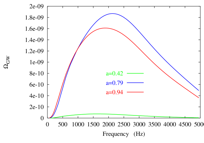
The value of $h_{0}^{2}\Omega_{\rm gw}$ has been computed in ref. [108] and is of order $10^{-10}$, peaked around 2 kHz. It is shown in fig. 16 (provided by the authors of ref. [108], and including a recent update of the star formation rate at large $z$) for three different values of the rotation parameter $a\equiv Jc/(GM^{2}_{\rm core})$, where $J$ is the angular momentum. A black hole forms only if $a$ is smaller than a critical value estimated in the range $a_{\rm crit}\sim 0.8-1.2$; otherwise rotational energy dominates, the star bounces, and no collapse occurs. For comparison with the other plots of $h_{0}^{2}\Omega_{\rm gw}$ shown in this report, note that fig. 16 shows $\Omega_{\rm gw}$ rather than $h_{0}^{2}\Omega_{\rm gw}$, and that ref. [108] uses $h_{0}=0.5$, so the value of $h_{0}^{2}\Omega_{\rm gw}$ is obtained from fig. 16 dividing by 4. Note also that both axes are on a linear scale, rather than a log-log scale, as the other plots that we show.

From the figure, we see that this background is out of reach for first generation experiments, while it could be detectable with advanced ground based interferometers.

It is also important to observe that the resulting GW signal is insensitive to the uncertainties that are present in the star formation rate in the high redshift region $z\sim 4-5$, since the result turns out to be dominated by low-to-intermediate redshift sources.

11.2 GWs from hydrodynamic waves in rotating neutron stars

In rapidly rotating neutron stars there is a whole class of instabilities driven by the emission of GWs, called CFS instabilities after Chandrasekhar [73], who discovered them, and Friedman and Schutz [122], who showed that they are generic to rotating neutron stars. Basically, they form when there is a mode that is forward-going, as seen from a distant observer, but backward going with respect to the rotation of the star. In this case, when this mode radiates away angular momentum, the star can find a rotation state with lower energy, than fueling further growth of the mode and therefore an instability occurs. Viscous forces, instead, tend to damp this instability.

Recent studies of rapidly rotating relativistic stars have revealed the existence of a particularly intersting class of modes (r-modes) that are unstable due to the emission of GWs [14, 121, 180]. As the star spins down, for these modes an energy of order of 1% of a solar mass is emitted in GWs, making the process very interesting for GW detection [207, 15]. Ref. [207] give a rough estimate of the spectrum assuming a comoving number density of neutron star births constant in the range $0<z<4$, and zero at higher $z$. A more detailed analysis has been done in ref. [109, 230], using again the star formation rate determined by observation, mentioned in the previous section. The analysis is performed for three different cosmological models, a flat Universe with vanishing cosmological constant ($\Omega_{M}=1,\Omega_{\Lambda}=0$) and $h_{0}=0.5$, a flat, low-density model ($\Omega_{M}=0.3,\Omega_{\Lambda}=0.7,h_{0}=0.6$), and an open model with $\Omega_{M}=0.4,\Omega_{\Lambda}=0,h_{0}=0.6$. Similarly to the computation of $R_{\rm NS}$ in the previous section, one can now compute the number of neutron stars formed per unit time within a comoving volume out at redshift $z$. Depending on the cosmological model, and on the upper cutoff in the progenitor mass, it turns out that

$$R_{\rm NS}\simeq(15-30)\,{\rm events/s}\,.$$ (255)

Comparing with the collapse to black hole, with the same parameters, one finds that $R_{\rm NS}\sim 4R_{\rm BH}$.

Figure 17: $h_{0}^{2}\Omega_{\rm gw}$ against frequency, for GWs produced by the r-mode of rotating neutron stars (from ref. [109]).

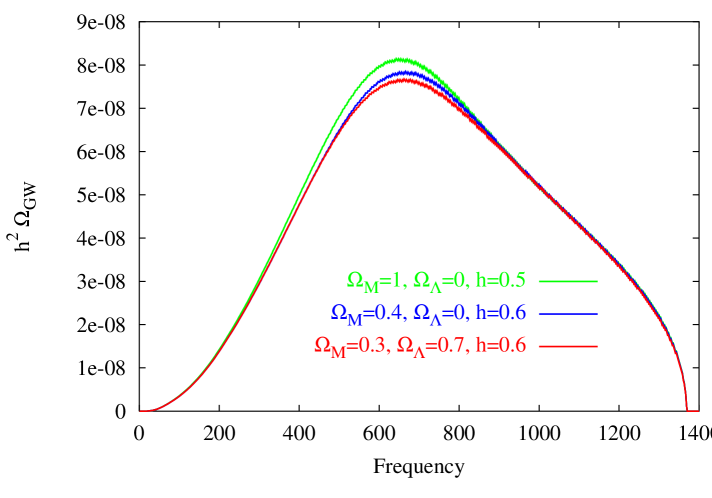
The mechanism of GW emission is discussed in refs. [180, 207, 15, 16]. The neutron star is modeled as a fluid with a polytropic equation of state $p=k\rho^{2}$, with $k$ chosen so that the mass of the neutron star is $1.4M_{\odot}$ and the radius is $R=12.53$ km. The r-mode excitation starts as a small perturbation of the velocity field. As long as the amplitude $\alpha$ of the r-mode us small, the effect of the instability is such that $\alpha$ grows exponentially while the angular velocity $\Omega$ of the neutron star is nearly constant. After approximately 500s, $\alpha$ becomes of order one, and we reach a regime where non-linear hydrodynamic effects are important. The non-linear effects saturate the growth of $\alpha$, which stays approximately constant. This phase lasts approximately for a time $\bar{\tau}_{\rm NS}\sim$ 1 yr, during which the star loses approximately 2/3 of its rotational energy by emission of GWs. Finally, the angular velocity becomes sufficiently low so that the r-mode ceases to be unstable.

Since GWs are emitted continuously over approximately 1yr, the duty cycle for this process is [109]

$$D=\int_{0}^{\infty}dR_{\rm NS}\,{\bar{\tau}}_{\rm NS}(1+z)\sim 10^{9}\,,$$ (256)

and therefore we definitely have a stochastic background.

The minimum and maximum values of the frequency radiated are estimated as follows [207]. It is known that the maximum possible angular velocity of a rotating star is

$$\Omega_{K}\sim 7.8\times 10^{3}\,{\rm Hz}\left[\frac{M}{M_{\odot}}\left(\frac{10\,{\rm km}}{R}\right)^{3}\right]^{1/2}\,,$$ (257)

where $M,R$ are the mass and radius of the corresponding non-rotating star. Assuming that most neutron stars are born with $\Omega$ close to $\Omega_{K}$, one can write the initial rotational energy of the star. Using the fact that about 2/3 of it is radiated into GWs, one finds

$$f_{\rm max}\simeq\frac{2}{3\pi}\Omega_{K}\,.$$ (258)

The lower cutoff in $f$ is associated to the fact that the r-mode instability becomes ineffective below some critical rotational frequency, and it can be estimated that

$$f_{\rm max}\simeq 120\,{\rm Hz}\,.$$ (259)

The resulting spectrum of GWs is shown in fig. 17, (provided by the authors of ref. [109], and including a recent update of the star formation rate at large $z$ and other technical improvements) for the three different cosmological models defined above. We see that the three curves are very similar, and therefore the result is quite solid against changes in the cosmological model, and [109]

$$h_{0}^{2}\Omega_{\rm gw}\simeq 8\times 10^{-8}$$ (260)

in the frequency range (500-700) Hz. This value is quite interesting, but from the discussion in sect. 6 it is clear that it is still below the sensitivities that can be obtained with correlations of first generation interferometers. It will be instead quite accessible to second generation experiments.

11.3 GWs from mass multipoles of rotating neutron stars

In the previous subsection we examined the case where GWs are emitted by rotating neutron stars through their coupling to the current multipoles associated to hydrodynamic waves on the star surface. We now discuss the emission by the simplest mechanism, which is the coupling of the GWs to the multipoles of the mass distribution of a rotating neutron star.

The stochastic background from mass multipoles of rotating neutron stars has been discussed in ref. [217]. The main uncertainty comes from the estimate of the typical ellipticity $\epsilon$ of the neutron star, which measures its deviation from sphericity. An upper bound on $\epsilon$ can be obtained assuming that the observed slowing down of the period of known pulsars is interely due to the emission of gravitational radiation. This is almost certainly a gross overestimate, since most of the spin down is probably due to electromagnetic losses, at least for Crab-like pulsars.

The typical frequency for these GWs can be in the range of ground-based interferometers. With realistic estimates for $\epsilon$, ref. [217] gives, at $f=100$ Hz, a value of $h_{c}(f)\sim 5\times 10^{-28}$, that, using eq. (19), corresponds to

$$h_{0}^{2}\Omega_{\rm gw}(100{\rm Hz})\sim 10^{-15}\,.$$ (261)

This is very far from the sensitivity of even the advanced experiments. An absolute upper bound can be obtained assuming that the spin down is due only to gravitational losses, and this gives $h_{0}^{2}\Omega_{\rm gw}(100{\rm Hz})\sim 10^{-7}$, but again this value is probably a gross overestimate.

Techniques for the detection of this background with a single interferometer using the fact that it is not isotropic and exploiting the sideral modulation of the signal have been discussed in ref. [133].

11.4 Unresolved galactic and extragalactic binaries

These backgrounds will be relevant in the LISA frequency band. For frequencies below a few mHz, one expects a stochastic background due to a large number of galactic white dwarf binaries [105, 37, 245, 231, 217, 36].

In sections (11.2,11.1), in order to determine whether the superposition of burst signals from supernovae formed a stochastic background, we used the duty cycle. For a continuous signal as that produced by binaries, instead, whether we have a stochastic background or not depends on our frequency resolution. After a time $T$ of observation, we can resolve $\Delta f=1/T$; for $T=$ 1 yr, $\Delta f\sim 3\times 10^{-8}$ Hz, and the number of resolvable frequencies in the LISA frequency band is of order $(1\,{\rm Hz})/(3\times 10^{-8}\,{\rm Hz})=3\times 10^{7}$. It is estimated that most frequency bins below a critical frequency of the order of 1 mHz will contains signal from more than one galactic binary, and will therefore form a confusion-limited background. Above this critical frequency, instead, individual signals will be resolved.

In particular, it is expected a contribution from compact white dwarf binaries. The computation of the intensity of this background depends on the rate of white dwarf mergers, which is uncertain. A possible estimate is shown in fig. 6 [36]. We see that, below a few mHz, it would cover a stochastic background of cosmological origin at the level $h_{0}^{2}\Omega_{\rm gw}\sim 10^{-11}$.

It should be observed that, even if an astrophysical background is present, and masks a relic background, not all hopes of observing the cosmological signal are lost. If we understand well enough the astrophysical background, we can subtract it, and the relic background would still be observable if it is much larger than the uncertainty that we have on the subtraction of the astrophysical background. In fact, LISA should be able to subtract the background due to white dwarf binaries, since there is a large number of binaries close enough to be individually resolvable [36]. This should allow to predict with some accuracy the space density of white dwarf binaries in other parts of the Galaxy, and therefore to compute the stochastic background that they produce. Furthermore, any background of galactic origin is likely to be concentrated near the galactic plane, and this is another handle for its identification and subtraction. The situation is more uncertain for the contribution of extragalactic binaries, which again can be relevant at LISA frequencies. The uncertainty in the merging rate is such that it cannot be predicted reliably, but it is believed to be lower than the galactic background [217]. In this case the only handle for the subtraction would be the form of the spectrum. In fact, even if the strength is quite uncertain, the form of the spectrum may be known quite well [36].

Finally, another possible astrophysical background can be expected if MACHO’s are black holes of mass $\sim 0.5M_{\odot}$ [204]. In this case we can expect that a large number of them will be in binary systems, and they could create a stochastic background relevant both for LISA and for ground-based interferometers [154].

12 Conclusions

Present GW experiments have not been designed especially for the detection of GW backgrounds of cosmological origin. Nevertheless, there are chances that in their frequency window there might be a cosmological signal. The most naive estimate of the frequency range for signals from the very early Universe singles out the GHz region, very far from the region accessible to ground based interferometers, $f<$ a few kHz, or to resonant masses. To have a signal in the accessible region, one of these two conditons should be met: either we find a spectrum with a long low-frequency tail, that extends from the GHz down to the kHz region, or we have some explosive production mechanism much below the Planck scale. As we have discussed, both situations seem to be not at all unusual, at least in the examples that have been worked out to date. The crucial point is the value of the intensity of the background.

With a very optimistic attitude, one could hope for a signal, with the maximum intensity compatible with the nucleosynthesis bound, $h_{0}^{2}\Omega_{\rm gw}\sim$ a few $\times 10^{-6}$ (or even $10^{-5}$, stretching all parameters to the maximum limit). Such an option is not excluded, and the fact that such a background is not predicted by the mechanisms that have been investigated to date is probably not a very strong objection, given our theoretical ignorance of physics at the Planck scale and the rate at which new production mechanisms have been proposed in recent years, see the reference list. However, with more realistic estimates, on general grounds it appears difficult to predict a background that, either in the region between a few Hz and a few kHz, relevant for ground based interferometers, or in the region $(10^{-4}-1)$ Hz relevant to LISA, exceeds the level $h_{0}^{2}\Omega_{\rm gw}\sim$ a few $\times 10^{-7}$, independently of the production mechanism. This should be considered the minimum detection level where a significant search can start. Such a level is beyond the sensitivity of first generation ground based detectors, but it is accessible both to advanced interferometers and to the space interferometer LISA.

The difficulties of such a detection are clear, but the payoff of a positive result would be enormous, opening up a window in the Universe and in fundamental high-energy physics that will never be reached with particle physics experiments.

Acknowledgments. I am grateful to Adalberto Giazotto for many interesting discussions and questions, which stimulated me to write down this report. I thank for useful discussions or comments on the manuscript Danilo Babusci, Stefano Braccini, Maura Brunetti, Alessandra Buonanno, Massimo Cerdonio, Eugenio Coccia, Viviana Fafone, Valeria Ferrari, Stefano Foffa, Maurizio Gasperini, Alberto Nicolis, Emilio Picasso, Raffaella Schneider, Riccardo Sturani, Carlo Ungarelli, Gabriele Veneziano and Andrea Vicerè.

I thank Barry Barish and Alberto Lazzarini for providing figs. 1 and 5, Karsten Danzmann and Roland Schilling for providing figs. (6,7). I thank Danilo Babusci for computing the overlap reduction functions and producing figs. (9,10), Viviana Fafone for providing fig. 8, and Raffaella Schneider and Valeria Ferrari for figs. (16,17).

I am grateful to Carl Gwinn for useful comments on sect. 7.4.

References

- [1] L. Abbott and D. Harari, Nucl. Phys. B264 (1986) 487.
- [2] L. Abbott and M. Wise, Phys. Lett. B135 (1984) 279.
- [3] L. Abbott and M. Wise, Nucl. Phys. B244 (1984) 541.
- [4] A. Abramovici et al., Science 256 (1992) 325.
- [5] F. Accetta and L. Krauss, Nucl. Phys. B319 (1989) 747.
- [6] A. Albrecht, R. Battye and J. Robinson, Phys. Rev. Lett. 79 (1997) 4736.
- [7] B. Allen, Phys. Rev. D37 (1988) 2078.
- [8] B. Allen, The Stochastic Gravity-Wave Background: Sources and Detection, in Les Houches School on Astrophysical Sources of Gravitational Waves, eds. J.A. Marck and J.P. Lasota, (Cambridge University Press, 1996); gr-qc/9604033.
- [9] B. Allen et al., gr-qc/9903108.
- [10] B. Allen and R. Brustein, Phys. Rev. D55 (1997) 3260.
- [11] B. Allen and S. Koranda, Phys. Rev. D50 (1994) 3713.
- [12] B. Allen and J. Romano, Phys. Rev. D59 (1999) 102001.
- [13] E. Amaldi and G. Pizzella, Nuovo Cim. 9C (1986) 612.
- [14] N. Andersson, Astrophys. J. 502 (1998) 708.
- [15] N. Andersson, K. Kokkotas and B. F. Schutz, astro-ph/9805225.
- [16] N. Andersson, K. Kokkotas and N. Stergioulas, astro-ph/9806089.
- [17] P. Astone et al., Europhysics Letters 12 (1990) 5.
- [18] P. Astone et al., Phys. Lett. B385 (1996) 421.
- [19] P. Astone et al., Astroparticle Phys. 7 (1997) 231.
- [20] P. Astone et al., Phys. Rev. D59 (1999) 122001.
- [21] P. Astone, J. Lobo and B. Schutz, Class. Quant. Grav. 11 (1994) 2093.
- [22] P. Astone, G. Pallottino and G. Pizzella, Class. Quant. Grav. 14 (1997) 2019.
- [23] P. Astone, S. Frasca, M.A. Papa and F. Ricci, Spectral detection strategy of Stochastic Gravitational Wave search in VIRGO, VIRGO note VIR-NOT-ROM-1390-106, Nov. 1997 (unpublished).
- [24] P. Astone, in Second Amaldi Conference on Gravitational Waves, E. Coccia, G. Pizzella and G. Veneziano eds., (World Scientific, Singapore, 1998), pg. 192
- [25] P. Astone et al., in Second Amaldi Conference on Gravitational Waves, E. Coccia, G. Pizzella and G. Veneziano eds., (World Scientific, Singapore, 1998), pg. 551.
- [26] P. Astone et al., Nucl. Phys. Proc. Suppl. 70 (1999) 461.
- [27] P. Avelino R. Caldwell and C. Martins, Phys. Rev. D56 (1997) 4568.
- [28] P. Avelino, E.P.S. Shellard, J.H.P. Wu and B. Allen, Phys. Rev. Lett. 81 (1998) 2008.
- [29] D. Babusci, S. Foffa, G. Losurdo, M. Maggiore, G. Matone and R. Sturani, The Stochastic Background, to appear as a chapter of the Virgo Data Analysis Document.
- [30] C. Baccigalupi, L. Amendola, P. Fortini and F. Occhionero, Phys. Rev. D56 (1997) 4610.
- [31] B. Barish, The detection of Gravitational Waves with LIGO, gr-qc/9905026.
- [32] B. Basset, Phys. Rev. D56 (1997) 3439.
- [33] R. Battye, R.R. Caldwell and E.P.S. Shellard, Gravitational waves from cosmic strings, astro-ph/9706013.
- [34] R. Battye, J. Robinson and A. Albrecht, Phys. Rev. Lett. 80 (1998) 4847.
- [35] B. Beinlich, F. Karsch and A. Peikert, Phys. Lett. B390 (1997) 268.
- [36] P. Bender et. al, LISA. Pre-Phase A Report, second edition, July 1998. A choice of reference texts on the LISA project can be found at http://www.lisa.uni-hannover.de/lisapub.html
- [37] P. Bender and D. Hils, Class. Quant. Grav. 14 (1997) 1439.
- [38] D. Bennet and F. Bouchet, Phys. Rev. D43 (1991) 2733.
- [39] C. Bennett et al., Astrophys. J. 464 (1996) L1.
- [40] Ph. Bernard, G. Gemme, R. Parodi and E. Picasso, Coupled microwave cavities for the detection of small harmonic displacement, Nota Interna INFN, INFN/TC-98/17, July 1998, (unpublished).
- [41] B. Bertotti, B. Carr and M. Rees, Mon. Not. R. Astron. Soc. 203 (1983) 945.
- [42] M. Bianchi, M. Brunetti, E. Coccia, F. Fucito, and J.A. Lobo, Phys. Rev. D57 (1998) 4525.
- [43] M. Bianchi, E. Coccia, C. Colacino, V. Fafone and F. Fucito, Class. Quant. Grav. 13 (1996) 2865;
- [44] N. Birrel and P.C.W. Davies, Quantum fields in curved space, Cambridge Univ. Press, Cambridge 1982.
- [45] D. Blair, E. Ivanov, M. Tobar, P. Turner, F. van Kann, and I. Heng, Phys. Rev. Lett. 74 (1995) 1908.
- [46] D. Blair, I. Heng, E. Ivanov, F. van Kann, N. Linthorne, M. Tobar and P. Turner, in Proc. of the Seventh Marcel Grossman Meeeting on General Relativity, (World Scientific, Singapore 1996), pg. 1446.
- [47] D. Blair and L. Ju, Mon. Not. R. Astron. Soc. 283 (1996) 648.
- [48] D. Blair and L. Ju, in Gravitational Waves; Sources and Detectors, I. Ciufolini and F. Fidecaro eds., Worlds Scientific 1997, pg. 193.
- [49] R. Blandford, R. Narayan and R. Romani, J. Astrophys. Astron. 5 (1984) 369.
- [50] D. Bodeker, P. John, M. Laine and M. Schmidt, Nucl. Phys. B497 (1997) 387.
- [51] V. Braginsky, N. Kardashev, A. Polnarev and I. Novikov, Nuovo Cim. 105B (1990) 1141.
- [52] A. Brignole, J. Espinosa, M. Quiròs and F. Zwirner, Phys. Lett. B324 (1994) 181.
- [53] A. Brillet for the Virgo collaboration, VIRGO- Status Report, November 1997, in Second Amaldi Conference on Gravitational Waves, E. Coccia, G. Pizzella and G. Veneziano eds., (World Scientific, Singapore, 1998), pg. 86.
- [54] M. Brunetti, E. Coccia, V. Fafone and F. Fucito, Phys. Rev. D59 (1999) 044027.
- [55] R. Brustein, in Gravitational Waves; Sources and Detectors, I. Ciufolini and F. Fidecaro eds., Worlds Scientific 1997, pg. 149.
- [56] R. Brustein, M. Gasperini, M. Giovannini and G. Veneziano, Phys. Lett. B361 (1995) 45.
- [57] R. Brustein, M. Gasperini and G. Veneziano, Phys. Rev. D55 (1997) 3882.
- [58] R. Brustein and M. Hadad, Phys. Rev. D57 (1998) 725.
- [59] R. Brustein and R. Madden, Phys. Lett. B410 (1997) 110, Phys. Rev. D57 (1998) 712, and hep-th/9901044.
- [60] R. Brustein and P. Steinhardt, Phys. Lett. B302 (1993) 196.
- [61] R. Brustein and G. Veneziano, Phys. Lett. B329 (1994) 429.
- [62] A. Buonanno, T. Damour and G. Veneziano, Nucl. Phys. B543 (1999) 275.
- [63] A. Buonanno, M. Maggiore and C. Ungarelli, Phys. Rev. D55 (1997) 3330.
- [64] A. Buonanno, K. Meissner, C. Ungarelli and G. Veneziano, JHEP01 (1998) 004.
- [65] G. Cagnoli, L. Gammaitoni, J. Kovalik, F. Marchesoni and M. Punturo, The VIRGO Sensitivity Curve, VIRGO Note VIR-NOT-PER-1390-84, Mar. 1997, (unpublished).
- [66] R. Caldwell and B. Allen, Phys. Rev. D45 (1992) 3447.
- [67] R.R. Caldwell, R. Battye and E.P.S.Shellard, Phys. Rev. D54 (1996) 7146.
- [68] M. Carena, M. Quiròs and C. Wagner, Phys. Lett. B380 (1996) 81; Nucl. Phys. B524 (1998) 3.
- [69] B. Caron et al., Class. Quant. Grav. 14 (1997) 1461.
- [70] B.J. Carr, Astron. Astrophys. 89 (1980) 6.
- [71] C.M. Caves, Phys. Lett. B80 (1979) 323.
- [72] M. Cerdonio et al., Class. Quant. Grav. 14 (1997) 1491.
- [73] S. Chandrasekhar, Phys. Rev. Lett. 24 (1970) 611.
- [74] N. Christensen, Phys. Rev. D46 (1992) 5250.
- [75] J. Cline and K. Kainulainen, Nucl. Phys. B482 (1996) 73.
- [76] E. Coccia, in Proceedings of the 14th International Conference on General Relativity and Gravitation, M. Francaviglia et al. eds., (World Scientific, Singapore, 1997), pg. 103;
- [77] E. Coccia, in Gravitational Waves; Sources and Detectors, I. Ciufolini and F. Fidecaro eds., Worlds Scientific 1997, pg. 201.
- [78] E. Coccia, V. Fafone, G. Frossati, J. Lobo and J. Ortega, Phys. Rev. D57 (1998) 2051.
- [79] E. Coccia, V. Fafone and I. Modena, Rev. Sci. Instr. 63 (1992) 5432.
- [80] E. Coccia, J. Lobo and J. Ortega, Phys. Rev. D52 (1995) 3735.
- [81] E. Coccia, G. Pizzella and F. Ronga, in Proceedings of the 1st Edoardo Amaldi Conf., (Frascati 1994), (World Scientific, Singapore 1995), pg. 161.
- [82] E. Coccia et al., Nucl. Instr. and Meth. A355 (1995) 624.
- [83] K. Compton and B. Schutz, Bar-Interferometer Observing, in Gravitational Waves; Sources and Detectors, I. Ciufolini and F. Fidecaro eds., Worlds Scientific 1997, pg. 173.
- [84] E. Copeland, E. Kolb, A. Liddle and J. Lidsey, Phys. Rev. D48 (1993) 2529.
- [85] E. Copeland, R. Easther and D. Wands, Phys. Rev. D56 (1997) 874.
- [86] E. Copeland, J. Lidsey, A. Liddle and D. Wands, Gen. Rel. Grav. 30 (1998) 1711; Phys. Rev. D58 (1998) 063508.
- [87] E. Copeland, J. Lidsey and D. Wands, Phys. Lett. B443 (1998) 97.
- [88] E. Copeland, J. Lidsey and D. Wands, Phys. Rev. D57 (1998) 625; Nucl. Phys. B506 (1997) 407.
- [89] C.J. Copi, D.N. Schramm and M.S. Turner, Phys. Rev. D55 (1997) 3389.
- [90] T. Damour, Experimental Tests of Relativistic Gravity, gr-qc/9904057.
- [91] T. Damour and N. Deruelle, Ann. Inst. H. Poincaré 44 (1986) 263.
- [92] T. Damour and G. Esposito-Farèse, Class. Quant. Grav. 9 (1992) 2093.
- [93] T. Damour and G. Esposito-Farèse, Phys. Rev. D58 (1998) 044003.
- [94] T. Damour and A.M. Polyakov, Nucl. Phys. B423 (1994) 532.
- [95] K. Danzmann for the LISA study team, Class. Quant. Grav. 14 (1997) 1399.
- [96] B. de Carlos and J. Espinosa, Nucl. Phys. B503 (1997) 24.
- [97] D. Delepine, J. Gerard, R. Gonzalez Felipe and J. Weyers, Phys. Lett. B386 (1996) 183.
- [98] R. DeSalvo, in Second Amaldi Conference on Gravitational Waves, E. Coccia, G. Pizzella and G. Veneziano eds., (World Scientific, Singapore, 1998), pg. 228.
- [99] S. Detweiler, Astrophys. J. 234 (1979) 1100.
- [100] R. Durrer, M. Gasperini, M. Sakellariadou and G. Veneziano, Phys.Lett. B436 (1998) 66; Phys.Rev. D59 (1999) 043511
- [101] R. Easther, K. Maeda and D. Wands, Phys. Rev. D53 (1996) 4247.
- [102] J. Espinosa, Nucl. Phys. B475 (1996) 273.
- [103] J. Espinosa, M. Quiròs and F. Zwirner, Phys. Lett. B307 (1993) 106.
- [104] F. Estabrook, Gen. Rel. Grav. 17 (1985) 719.
- [105] C. Evans, I. Iben and L. Smarr, Astrophys. J. 323 (1987) 129.
- [106] R. Fabbri and M.D. Pollock, Phys. Lett. 125B (1983) 445.
- [107] G. Farrar and M. Losada, Phys. Lett. B406 (1997) 60.
- [108] V. Ferrari, S. Matarrese and R. Schneider, Mon. Not. R. Astron. Soc. 303 (1999) 247.
- [109] V. Ferrari, S. Matarrese and R. Schneider, Mon. Not. R. Astron. Soc. 303 (1999) 258.
- [110] V. Ferrari and C. Palomba, Int. J. Mod. Phys. D7 (1998) 825.
- [111] L. Finn, Lectures given at 26th SLAC Summer Institute on Particle Physics: Gravity – From the Hubble Length to the Planck Length (SSI 98), Stanford, CA, 3-14 Aug 1998, gr-qc/9903107
- [112] D. J. Fixsen et al., Astrophysics J. 473 (1996) 576.
- [113] E. Flanagan, Phys. Rev. D48 (1993) 2389.
- [114] S. Foffa, M. Maggiore and R. Sturani, Phys. Rev. D59 (1999) 043507.
- [115] S. Foffa, M. Maggiore and R. Sturani, Nucl. Phys. B552 (1999) 395.
- [116] R. Forster and D. Backer, Astrophys. J. 361 (1990) 300.
- [117] R. Forward, Gen. Relativ. Gravit. 2 (1971) 149.
- [118] R. Forward, Phys. Rev. D17 (1978) 379.
- [119] S. Frasca and M.A. Papa, in Proceedings of the First Amaldi Conference on Gravitational Wave Experiment, (World Scientific, Singapore, 1995), pag. 436-448.
- [120] S. Frasca, in Second Amaldi Conference on Gravitational Waves, E. Coccia, G. Pizzella and G. Veneziano eds., (World Scientific, Singapore, 1998), pg. 216.
- [121] J. Friedman and S. Morsink, Astrophys. J. 502 (1998) 714.
- [122] J. Friedman and B. Schutz, Astrophys. J. 222 (1978) 281.
- [123] M. Gasperini, in ”Proc. of the 12th Italian Conference on Gen. Rel. and Gravitational Physics” (Rome, September 1996), ed. by M. Bassan et al. (World Scientific, Singapore), p.181.
- [124] M. Gasperini, in Second Amaldi Conference on Gravitational Waves, E. Coccia, G. Pizzella and G. Veneziano eds., (World Scientific, Singapore, 1998), pg. 62
- [125] M. Gasperini, Phys. Rev. D56 (1997) 4815.
- [126] M. Gasperini and M. Giovannini, Phys. Lett. B282 (1992) 36; Phys. Rev. D47 (1993) 1519.
- [127] M. Gasperini, M. Giovannini and G. Veneziano, Phys. Rev. D48 (1993) R439.
- [128] M. Gasperini, M. Maggiore and G. Veneziano, Nucl. Phys. B494 (1997) 315.
- [129] M. Gasperini, J. Maharana and G. Veneziano, Nucl. Phys. B472 (1996) 349.
- [130] M. Gasperini and G. Veneziano, Astropart. Phys. 1 (1993) 317; Mod. Phys. Lett. A8 (1993) 3701. An up-to-date collection of references on string cosmology can be found at http://www.to.infn.it/teorici/~gasperin/
- [131] M. Gasperini and G. Veneziano, Phys. Rev. D50 (1994) 2519.
- [132] M. Gasperini and G. Veneziano, Phys. Lett. B387 (1996) 715.
- [133] A. Giazotto, S. Bonazzola and E. Gourgoulhon, Phys. Rev. D55 (1997) 2014.
- [134] G.F. Giudice, Phys. Rev. D45 (1992) 3177.
- [135] M. Gleiser, Phys. Rev. Lett. 63 (1989) 1199.
- [136] M. Gleiser and R. Roberts, Phys. Rev. Lett. 81 (1998) 5497.
- [137] A.M. Green, A.R. Liddle and A. Riotto, Phys. Rev. D56 (1997) 7559.
- [138] L.P. Grishchuk, Sov. Phys. JETP, 40 (1975) 409.
- [139] L.P. Grishchuk, Class. Quant. Grav. 10 (1993) 2449.
- [140] L. Grishchuk, Class. Quant. Grav. 14 (1997) 1445.
- [141] C. Gwinn, M. Eubanks, T. Pyne, M. Birkinshaw and D. Matsakis, Astrophys. J. 485 (1997) 87.
- [142] W. Hamilton, The Allegro detector and the future of resonant detectors in the USA, in Second Amaldi Conference on Gravitational Waves, E. Coccia, G. Pizzella and G. Veneziano eds., (World Scientific, Singapore, 1998), pg. 115.
- [143] R. Hellings and G. Downs, Astrophys. J. 265 (1983) L39.
- [144] I. Heng, D. Blair, E. Ivanov and M. Tobar, Phys. Lett. A218 (1996) 190.
- [145] I. Heng, D. Blair, E. Ivanov and M. Tobar, in Second Amaldi Conference on Gravitational Waves, E. Coccia, G. Pizzella and G. Veneziano eds., (World Scientific, Singapore, 1998), pg. 127.
- [146] M.B. Hindmarsh and T.W.B. Kibble, Rep. Prog. Phys. 58 (1995) 477.
- [147] C. Hogan, Phys. Lett B133 (1983) 172.
- [148] C. Hogan, Mon. Not. R. Astr. Soc. 218 (1986) 629.
- [149] C. Hogan, astro-ph/9809364.
- [150] J. Hough for the LISA SCINCE TEAM, in Second Amaldi Conference on Gravitational Waves, E. Coccia, G. Pizzella and G. Veneziano eds., (World Scientific, Singapore 1998), pg. 97.
- [151] R. Hulse and J. Taylor, Astrophys. J. 324 (1975).
- [152] J. Hwang, Class. Quant. Grav. 15 (1998) 1401.
- [153] E. Iacopini, E. Picasso, F. Pegoraro and L.A. Radicati, Phys. Lett. A73 (1979) 140.
- [154] K. Ioka, T. Tanaka and T. Nakamura, Phys. Rev. D60 (1999) 083512.
- [155] Y. Iwasaki et al., Z. Phys. C71 (1996) 343.
- [156] Y. Iwasaki et al., Phys. Rev. D49 (1994) 3540.
- [157] W. Johnson and S. Merkowitz, Phys. Rev. Lett. 70 (1993) 2367.
- [158] N. Kaiser and A. Jaffe, Astrophys. J. 484 (1997) 545.
- [159] D. Kalligas and R. Wagoner, Resonant-Mass Detection of Tensor and Scalar Waves, in ”Relativistic Gravitation and Gravitational Radiation” (Les Houches 1995), edited by J.-A. Marck and J.-P. Lasota (Cambridge University Press, 1997), pg. 433.
- [160] N. Kaloper, R. Madden and K. Olive, Nucl. Phys. B452 (1995) 677.
- [161] V. Kaplunovsky, Phys. Rev. Lett. 55 (1985) 1036.
- [162] V. Kaspi, J. Taylor and M. Ryba, Astrophys. J. 428 (1994) 713.
- [163] K. Kawabe and the TAMA collaboration, Class. Quant. Grav. 14 (1997) 1477.
- [164] M. Kawasaki and T. Moroi, Progr. Theor. Phys. 93 (1995) 879.
- [165] C. Keeton and C. Kochanek, Astrophys. J. 487 (1997) 42.
- [166] S. Khlebnikov and I. Tkachev, Phys. Rev. D56 (1997) 653.
- [167] L. Kofman, A. Linde and A. Starobinsky, Phys. Rev. Lett. 73 (1994) 3195; ibid., 76 (1996) 1011; Phys. Rev. D56 (1997) 3258.
- [168] E.W. Kolb and M.S. Turner, The Early Universe, Addison Wesley 1990.
- [169] S. Kopeikin, Phys. Rev. D56 (1997) 4455.
- [170] M. Kamionkowski, A. Kosowsky and M. Turner, Phys. Rev. D49 (1994) 2837.
- [171] A. Kosowsky and M. Turner, Phys. Rev. D47 (1993) 4372.
- [172] A. Kosowsky and M. Turner, Phys. Rev. D52 (1995) R1739.
- [173] L. Krauss, Phys. Lett. B284 (1992) 229.
- [174] L. Krauss and M. White, Phys. Rev. Lett. 69 (1992) 869.
- [175] M. Laine, Nucl. Phys. B481 (1996) 43.
- [176] M. Laine and K. Rummukainen, Phys. Rev. Lett. 80 (1998) 5259; hep-lat/9804019.
- [177] The LIGO Scientific Collaboration, LSC White Paper on Detector Research and Developement, Nov. 1998, internal document of the LIGO collaboration.
- [178] A. Liddle and M. Turner, Phys. Rev. D50 (1994) 758.
- [179] J.E. Lidsey, D. Wands and E.J. Copeland, Superstring cosmology, hep-th/9909061.
- [180] L. Lindblom, B. Owen and S. Morsink, Phys. Rev. Lett 80 (1998) 4843.
- [181] E. Linder, Astrophys. J. 328 (1988) 77.
- [182] J.A. Lobo, Phys. Rev. D52 (1995) 591.
- [183] M. Losada, Phys. Rev. D56 (1997) 2893; hep-ph/9806519.
- [184] D. Lorimer, Binary and Millisecond Pulsars, in Living Reviews in Relativity, available electronically at www.livingreviews.org/Articles/Volume1/1998-10lorimer.
- [185] H. Lück and the GEO600 Team, Class. Quant. Grav. 14 (1997) 1471. See also http://www.geo600.uni-hannover.de/
- [186] D. Lyth and A. Riotto, Particle Physics Models of Inflation and the Cosmological Density Perturbation, hep-th/9807278, to appear in Phys. Rept.
- [187] M. Maggiore, Nucl. Phys. B525 (1998) 413.
- [188] M. Maggiore, Phys. Rev. D56 (1997) 1320.
- [189] M. Maggiore and A. Nicolis, Detection strategies for scalar gravitational waves with interferometers and resonant spheres, gr-qc/9907055.
- [190] M. Maggiore and A. Riotto, Nucl. Phys. B548 (1999) 427.
- [191] M. Maggiore and R. Sturani, Phys. Lett. B415 (1997) 335.
- [192] X. Martin and A. Vilenkin, Phys. Rev. Lett. 77 (1996) 2879.
- [193] E. Mauceli, Z.K. Geng, W.O. Hamilton, W.W. Johnson, S. Merkowitz, A. Morse, B. Price, N. Solomonson Phys. Rev. D54 (1996) 1264.
- [194] G. Mazzitelli and M.A. Papa, Interaction of high energy muons and hadrons with a large aluminum spherical resonant detector, Presented at OMNI 1: 1st International Workshop on an Omnidirectional Gravitational Radiation Observatory, Sao Jose dos Campos, Brazil, 26-31 May 1996.
- [195] A. Melchiorri, M.V. Sazhin, V.V. Shulga and N. Vittorio, Astrophys. J. 518 (1999) 562.
- [196] A. Melchiorri, F. Vernizzi, R. Durrer and G. Veneziano, Cosmic microwave background anisotropies and extra dimensions in string cosmology, astro-ph/990532.
- [197] L. Mendes and A. Liddle, Early cosmology and the stochastic gravitational wave background, gr-qc 9811040.
- [198] S. Merkowitz and W. Johnson, Phys. Rev. D51 (1995) 2546, Phys. Rev. D53 (1996) 5377, Phys. Rev. D56 (1997) 7513.
- [199] S. Merkowitz and W. Johnson, Europhys. Lett. 41 (1998) 355.
- [200] P. Michelson, Mon. Not. Roy. Astron. Soc. 227 (1987) 933.
- [201] C. Misner, K. Thorne and J. Wheeler, Gravitation, Freeman, N.Y., 1973.
- [202] V. F. Mukhanov, H. A. Feldman and R. H. Brandenberger, Phys. Rept. 215 (1992) 203.
- [203] S. Myint, Phys. Lett B287 (1992) 325.
- [204] T. Nakamura, M. Sasaki, T. Tanaka and K. Thorne, Astrophys. J. 487 (1997) L139.
- [205] D. Nicholson et al., Phys. Lett. A218 (1996) 175.
- [206] A. Nicolis, Tesi di Laurea, Università di Pisa, May 1999 (unpublished).
- [207] B. Owen, L. Lindblom, C. Cutler, B. F. Schutz, A. Vecchio, N. Andersson, Phys. Rev. D58 (1998) 084020.
- [208] G. Pallottino, in Gravitational Waves; Sources and Detectors, I. Ciufolini and F. Fidecaro eds., Worlds Scientific 1997, pg. 159.
- [209] Particle Data Group, Review of Particle Properties, Phys. Rev. D50 (1994) 1173.
- [210] J. Polchinski, String Theory, Cambridge University Press, Cambridge 1998.
- [211] F. Pegoraro, E. Picasso and L.A. Radicati, J. Phys. A 11 (1978) 1949.
- [212] F. Pegoraro and L. A. Radicati, J. Phys. A 13 (1980) 2411.
- [213] F. Pegoraro, L.A. Radicati, Ph. Bernard and E. Picasso, Phys. Lett. A 68 (1978) 165.
- [214] U. Pen, U. Seljak and N. Turok, Phys. Rev. Lett. 79 (1997) 1615.
- [215] G. Pizzella, Class. Quant. Grav. 14 (1997) 1481.
- [216] G. Pizzella, Do cosmic rays perturb the operation of a large resonant spherical detector of gravitational waves?, preprint LNF-99/001(IR), Laboratori Nazionali di Frascati, Jan. 1999 (unpublished).
- [217] K. Postnov, Astrophysical Sources of Stochastic Gravitational Radiation in the Universe, astro-ph/9706053.
- [218] G.A. Prodi et al., in Gravitational Waves; Sources and Detectors, I. Ciufolini and F. Fidecaro eds., Worlds Scientific 1997, pg. 166.
- [219] G.A. Prodi et al., in Second Amaldi Conference on Gravitational Waves, E. Coccia, G. Pizzella and G. Veneziano eds., (World Scientific, Singapore 1998), pg. 148.
- [220] A. Riotto and M. Trodden, hep-ph/9901362
- [221] C. Reece, P. Reiner and A. Melissinos, Phys. Lett. 104A (1984) 341; Nucl. Instr. Meth. A245 (1986) 299.
- [222] R. Romani and J. Taylor, Astrophys. J. 265 (1983) L35.
- [223] V. Rubakov, M. Sazhin and A. Veryaskin, Phys. Lett. 115B (1982) 189.
- [224] R. Sachs and A. Wolfe, Astrophys. J. 147 (1967) 73.
- [225] V. Sahni, Phys. Rev. D42 (1990) 453.
- [226] A. Sandage et. al., Astrophys. J. 460 (1996) L15.
- [227] R. Sandeman, in Second workshop on gravitational waves data analysis, M. Davier and P. Hello eds., Èditions Frontiéres, Paris, 1998.
- [228] M. Sazhin, Sov. Astron. 22 (1978) 36.
- [229] C. Schmid, D. Schwarz and P. Widerin, Phys. Rev. D59 (1999) 043517.
- [230] R. Schneider, V. Ferrari and S. Matarrese, to be published in the proceedings of 19th Texas Symposium on Relativistic Astrophysics: Texas in Paris, Paris, France, 14-18 Dec 1998, astro-ph/9903470.
- [231] B.F. Schutz, Low-Frequency Sources of Gravitational Waves: a tutorial, in Proceedings of the 1997 Alpbach Summer School on Fundamental Physics in Space, ed. A. Wilson, ESA (1997), to be published.
- [232] B. Schutz and M. Tinto, Mon. Not. R. Astr. Soc., 224 (1987) 131.
- [233] V.F. Schwartzmann, JETP Lett. 9 (1969) 184.
- [234] D.J. Schwarz, Mod. Phys. Lett. A13 (1998) 2771.
- [235] T. Souradeep and V. Sahni, Mod. Phys. Lett. A7 (1992) 3541.
- [236] A. Starobinski, JETP Lett. 30 (1979) 682.
- [237] P. Steinhardt, Phys. Rev. D25 (1982) 2082.
- [238] T. Stevenson, Phys. Rev. D56 (1997) 564.
- [239] E. Stewart and D. Lyth, Phys. Lett. B302 (1993) 171.
- [240] D. Stinebring, M. Ryba, J. Taylor and R. Romani, Phys. Rev. Lett. 65 (1990) 285.
- [241] J. Taylor, Rev. Mod. Phys. 66 (1994).
- [242] J. Taylor and J. Weisberg, Astrophys. J. 253 (1982) 908; ibid. 345 (1989) 434.
- [243] M. Tegmark and J. Silk, Astrophys. J. 441 (1995) 458.
- [244] K.S. Thorne, in 300 Years of Gravitation, S. Hawking and W. Israel eds., Cambridge University Press, Cambridge, 1987.
- [245] K.S. Thorne, in Proceedings of Snowmass 1994 Summer Study on Particle and Nuclear Astrophysics and Cosmology, E. Kolb and R. Peccei eds., World Scientific, Singapore, 1995, pg. 398.
- [246] S. Thorsett and R. Dewey, Phys. Rev. D53 (1996) 3468.
- [247] R. Tripp, Astronomy and Astrophys. 325 (1997) 871.
- [248] M. Turner, Ten Things Everyone Should Know About Inflation, astro-ph/9704062.
- [249] M. Turner, Phys. Rev. D55 (1997) 435. v
- [250] M. Turner, E. Weinberg and L. Widrow, Phys. Rev. D46 (1992) 2384.
- [251] M. Turner, M. White and J. Lidsey, Phys. Rev. D48 (1993) 4613.
- [252] M. Turner and F. Wilczek, Phys. Rev. Lett. 65 (1990) 3080.
- [253] G. Veneziano, Phys. Lett. B265 (1991) 287.
- [254] A. Vilenkin, Phys. Lett. B107 (1981) 47; Phys. Rept. 121 (1985) 263.
- [255] A. Vilenkin and E.P.S. Shellard, Cosmic Strings and other Topological Defects, Cambridge Univ. Press, Cambridge 1994.
- [256] The VIRGO collaboration, Final Design Report, VIR-TRE-1000-13, May 1997 (unpublished).
- [257] S. Vitale, M. Cerdonio, E. Coccia and A. Ortolan, Phys. Rev. D55 (1997) 1741.
- [258] R. Wagoner, Resonant-Mass Detection of Tensor and Scalar Waves, in ”Relativistic Gravitation and Gravitational Radiation” (Les Houches 1995), edited by J.-A. Marck and J.-P. Lasota (Cambridge University Press, 1997), pg. 419.
- [259] R. Wagoner and H. Paik, in Experimental Gravitation, Proceedings of the Pavia International Symposium (Accademia Nazionale dei Lincei, Roma, Italy, 1977), pg. 257.
- [260] E. Witten, Phys. Rev. D30 (1984) 272.
- [261] C.Z. Zhou and P. Michelson, Phys. Rev. D51 (1995) 2517.
- [262] J. Zibin, D. Scott and M. White, astro-ph/9904228.
- [263] D. Zipoy and B. Bertotti, Nouvo Cim. 56B (1968) 195.