The Asymptotic Behaviour of Cosmological Models Containing Matter and Scalar Fields

132E 1326

THE ASYMPTOTIC BEHAVIOUR OF COSMOLOGICAL MODELS CONTAINING MATTER AND SCALAR FIELDS

By
Andrew Philip Billyard

SUBMITTED IN PARTIAL FULFILLMENT OF THE
REQUIREMENTS FOR THE DEGREE OF
DOCTOR OF PHILOSOPHY
AT
DALHOUSIE UNIVERSITY
HALIFAX, NOVA SCOTIA
MARCH 2024

© Copyright by Andrew Philip Billyard, 2024

DALHOUSIE UNIVERSITY

DEPARTMENT OF

PHYSICS

The undersigned hereby certify that they have read and recommend to the Faculty of Graduate Studies for acceptance a thesis entitled “The Asymptotic Behaviour of Cosmological Models Containing Matter and Scalar Fields” by Andrew Philip Billyard in partial fulfillment of the requirements for the degree of Doctor of Philosophy.

Dated:  March 2024 

External Examiner:

  Kayll Lake

Research Supervisor:

  Alan A. Coley

Examing Committee:

  H. Jürgen Kreuzer

  D.J. Wallace Geldart

DALHOUSIE UNIVERSITY

Date: March 2024

• Andrew Philip Billyard

• The Asymptotic Behaviour of Cosmological Models Containing Matter and Scalar Fields

• Physics

Degree: Ph.D. Convocation: October Year: 1999

Permission is herewith granted to Dalhousie University to circulate and to have copied for non-commercial purposes, at its discretion, the above title upon the request of individuals or institutions.

  Signature of Author

THE AUTHOR RESERVES OTHER PUBLICATION RIGHTS, AND NEITHER THE THESIS NOR EXTENSIVE EXTRACTS FROM IT MAY BE PRINTED OR OTHERWISE REPRODUCED WITHOUT THE AUTHOR’S WRITTEN PERMISSION.

THE AUTHOR ATTESTS THAT PERMISSION HAS BEEN OBTAINED FOR THE USE OF ANY COPYRIGHTED MATERIAL APPEARING IN THIS THESIS (OTHER THAN BRIEF EXCERPTS REQUIRING ONLY PROPER ACKNOWLEDGEMENT IN SCHOLARLY WRITING) AND THAT ALL SUCH USE IS CLEARLY ACKNOWLEDGED.

Abstract

The asymptotic behaviour of two classes of scalar field cosmological models are studied using the theory of dynamical systems: general relativistic Bianchi models containing matter and a scalar field with an exponential potential and a class of spatially homogeneous string cosmological models. The purpose of this thesis is to examine some of the outstanding problems which currently exist in cosmology, particularly regarding isotropization and inflation. It is shown that the matter scaling solutions are unstable to curvature perturbations. It is then shown that the Bianchi class B exponential potential models can alleviate the isotropy problem; an open set of models within this class do isotropize to the future. It is also shown that the presence of an interaction term in the subclass of isotropic models can lead to inflationary models with late-time oscillatory behaviour in which the matter is not driven to zero. Next, within the class of the string cosmologies studied, it is shown that there is a subclass which do not inflate at late times in the post-big bang regime. Furthermore, all string models studied typically do not have a late–time flatness problem. Indeed, it is shown that curvature typically plays an important rôle only at intermediate times in most models. It is also shown that the presence of a positive cosmological constant in the models studied can lead to interesting physical behaviour, such as multi-bouncing universes. A mathematical equivalence between general relativistic scalar field theories and scalar-tensor theories and string theories has been extensively exploited and thus the results obtained from the string analysis compliment the results obtained from the Bianchi class B exponential potential analysis.

List of Symbols

$a=e^{\alpha}$ scale factor
$\{\tilde{A}\equiv\frac{\tilde{a}}{9H^{2}},~{}N_{+}\equiv\frac{n_{+}}{3H}\}$ normalized curvature terms
$c$ speed of light
$g_{\alpha\beta}$ metric
$G$ gravitational (Newton’s) constant
$G_{\alpha\beta}$ Einstein tensor
$H\equiv\dot{\alpha}=\frac{1}{3}\theta$ Hubble parameter
$k$ exponential potential paramter $V=V_{0}e^{k\phi}$
$\{\tilde{K},K\}$ curvature terms
$l=h^{-1}$ Bianchi type VI_h and VII_h parameter
$p$ pressure
$q$ deceleration parameter
$Q$ Ramond–Ramond parameter
$R$ Ricci scalar
$R_{\alpha\beta}$ Ricci tensor
$\{s,t,T,\tau,\eta\}$ time
$T_{\alpha\beta}$ energy-momentum tensor
$u_{\alpha}$ fluid velocity
$U$ scalar field potential in Jordan frame
$V$ scalar field potential in Einstein frame
$\{u,U_{i},v,V_{i},x,X_{i},y,Y_{i},z,Z_{i}\}$ normalized phase space variables

$\beta_{m}$ modulus field
$\beta_{s}$ shear
$\beta$ $\dot{\beta}_{s}^{2}+6\dot{\beta}_{m}^{2}$
$\delta$ interaction term
$\Delta$ normalized shear and curvature term
$\gamma$ equation of state parameter
$\Gamma^{\alpha}_{\beta\delta}$ affine connection
$\{\zeta_{i},\kappa,\lambda_{i},\mu_{i},\nu_{i},\xi_{i},\chi_{i}\}$ phase space variables
$\Lambda$ central charge deficit
$\Lambda_{\rm M}$ cosmological constant
$\mu\equiv 3H\Omega$ energy density
$\sigma$ axion field
$\rho$ axion field energy density
$\{\Sigma_{+}\equiv\frac{\sigma_{+}}{3H},~{}\tilde{\Sigma}\frac{\tilde{\sigma}}{9H^{2}}\}$ normalized shear terms
$\phi$ scalar field in Einstein frame
$\varphi\equiv\hat{\Phi}-3\alpha$ shifted dilaton field
$\Psi\equiv\frac{\dot{\phi}}{\sqrt{6}H}$ normalized scalar field variable
$\Phi\equiv e^{-\hat{\Phi}}$ scalar field in Jordan frame
$\Upsilon\equiv\frac{\sqrt{V}}{\sqrt{3}H}$ normalized potential variable

Chapter 1 Introduction

1.1 Current Issues in Cosmology

With the birth of the theory of relativity, ideas in cosmology went through a great reformation. The advent of special relativity removed the notion of an absolute “inertial” spatial reference frame in which the sequence of events were measured by a concept of time identical for all observers. Furthermore, when general relativity was formulated the physical arena was now considered to be a four-dimensional spacetime in which measurements of an event not only depended on the relative motions of the observers, but also on the gravitational field present, and gravity was now considered in geometrical terms; objects moving under the influence of gravity were considered to be following specific four-dimensional paths on a manifold whose curvature is induced by the presence of matter. Because special relativity brought to light the equivalence between mass and energy, this matter source could include a bath of radiation (in which the constituent components are massless). The universe, previously static with neither beginning nor end, was now modeled by a dynamic theory formulated within the mathematical framework of general relativity, namely pseudo-Riemannian geometry. However, the cosmological reformation that had transpired at the birth of general relativity did not cease thereafter, and the issues of cosmology lead to an active field of research to this day, and hereby the issues of great importance are discussed.

It is known that on the largest observable scales, the universe appears to be spatially isotropic and spatially homogeneous. Observational support for spatial isotropy comes from the Cosmic Background Explorer (COBE) data, where measured anisotropies of the microwave background radiation are only 1 part in $10^{5}$ [1, 2, 3, 4, 5, 6]. Support for spatial homogeneity come from galaxy distributions [7, p. 39] and partially from nuclear abundances [8, 9, 10, 11]. However, homogeneity is mostly a theoretical assumption based on the Copernican principle [12, p. 407] that we’re not in a preferred location in the universe; if the universe appears homogeneous from our point of view, then it is assumed to be homogeneous from any point of view. If a space is isotropic about all points in a space-like hypersurface then it must be spatially homogeneous [13, p. 109]. Partial support for homogeneity can also come from the COBE data. Cosmological models with such properties are described by the Friedmann–Robertson–Walker (FRW) models. Once these models are assumed to describe the universe, it is possible to measure the values of the Hubble parameter, $H_{0}$, (a measure of the universe’s expansion rate; here the subscript “0” refers to such values at the current epoch) and the deceleration parameter, $q_{0}$ (a unitless quantity which measures the expansion’s acceleration; $q<0$ implies an accelerated expansion whilst $q>0$ describes a decelerated expansion). Such measurements lead to information about the universe, such as its curvature or the value of the cosmological constant (if one is present). The FRW models have a lot of predictive power. Not only do they lead to the Hubble law at low redshift (which states that the ratio of redshift to distance is equal to $H$, see equation (1.16) on page 1.16), but they predict a hot Big-Bang which is compatible with the observed microwave background radiation and observed nucleosynthesis yields, and which predicts a possible neutrino background [12, Ch. 15.6]. However, it would seem that there are presently several potential problems that arise when the FRW models are used.

The primary issue associated with this thesis is that the FRW models do not explain the observed isotropy of the universe, but rather this property is assumed. The isotropy condition may be relaxed and one of the spatially homogeneous (but spatially anisotropic) Bianchi models or Kantowski-Sacks model can be used. In doing so, it has been shown that these models do not always isotropize. In particular, models of Bianchi type IX recollapse [14] and do not necessarily isotropize [15]. Furthermore, Collins and Hawking [16] have shown that there is a zero measure of spatially homogeneous models containing ordinary matter which can isotropize as $t\rightarrow\infty$; this implies that the conditions of the universe currently observed are not generic within this class of models. This is referred to as the isotropy issue, and will be one of the main foci of this thesis. Recently it has been shown [17] that for a particular Bianchi VII₀ model the fluid’s shear terms became negligible at late times, but anisotropies in the Weyl curvature tensor became dominant and so the model does not isotropize. However, such models of this type are not considered within this thesis, and isotropy effectively occurs when the fluid’s shear vanishes.

The issue of spatial homogeneity also implies a few potential problems. First of all, small perturbations from spatial homogeneity would be needed to seed the formation of galaxies and stars. However, FRW models without a cosmological constant predict that the largest possible age of the universe is $H_{0}^{-1}$; using FRW models, data suggests that the universe began less than $10^{10}/h_{0}$ years ago (since data suggests values of $H_{0}\approx 50-100km/s/Mpc$ the Hubble parameter is often written $H_{0}=h_{0}\times 100km/s/Mpc$ with $h_{0}\in[\frac{1}{2},1]$), yet some of the oldest globular clusters are in the age range $10\times 10^{9}$ to $13\times 10^{9}$ years [18, 19] (in [18] it was stated with 95% confidence that the minimum age of the universe is $9.5\times 10^{9}$ years based on the ages of globular clusters) and so there may be a discrepancy between observation and theory. Recently, a value of $h_{0}=0.7\pm 0.07$ (corresponding to an age of $13\times 10^{9}$ to $15\times 10^{9}$ years in the FRW models) has been suggested [20, 21], although this value is under much debate [21]. This potential discrepancy can be easily resolved, even within FRW models, by including a scalar field with a potential (or even just a cosmological constant); with such a field present the models may go through a period of accelerated expansion and hence $H_{0}^{-1}$ cannot be used to determine the upper age of the model. This type of behaviour is typical of the models considered within this thesis.

Another problem with standard FRW models is associated with particle horizons, which is the distance travelled by light since the time of the Big Bang. Since the ages of standard FRW model universes are finite, there are regions of space which are outside of each other’s particle horizons and hence have never been in causal contact, and consequently there is no reason why they should have evolved in the same manner. However, it is very easy to observe two regions of space which are causally disconnected from each other and yet appear the same; both have formed galaxies and clusters of galaxies and super-clusters etc., the distributions of which appear similar, and the measured anisotropies in the microwave background radiation is the same. Hence, it would seem natural to assume that sometime in the past these regions had been in causal contact. This is known as the horizon problem.

Another issue is the flatness problem which involves the critical density parameter, $\Omega$, which is proportional to the ratio of energy density of the universe to it’s expansion rate; for $\Omega>1$ the energy content of the universe eventually causes a recollapse, for $\Omega<1$ there is insufficient matter to halt the expansion and for critical value $\Omega=1$ the universe stops expanding as $t\rightarrow\infty$. In FRW models, $\Omega$ is linearly proportional to the universe’s curvature $k$ (see section 1.2), and in particular $k=0$ corresponds to $\Omega=1$. The flatness problem is so called because the FRW models do not explain why current data suggests $0.1<\Omega<10$; that is, near $\Omega\approx 1$ ($k=0$). Unless $k=0$ exactly, it would be expected for the current epoch that $\Omega\approx 0$ for open ($k<0$) models or $\Omega\gg 1$ for closed ($k>0$) models.

Note that these problems (isotropy, particle horizon and flatness) are related to one another [22]. Many of these problems may be alleviated within the inflationary scenario, a paradigm in which the universe undergoes an accelerated expansion at an early epoch ($q<0$). In such a scenario, a universe could very well be inhomogeneous and anisotropic, but the current observable portion of that universe was originally a small causally connected region of the entire universe, which has inflated [23, 24]. Hence, inhomogeneities could have been pushed outside our observable universe whilst allowing present, causally disconnected parts of the universe to have been connected in the past, solving the horizon problem. This mechanism could also explain the flatness problem, since it is possible for inflation to drive the universe towards $\Omega=1$, although not all inflationary models will do this (indeed, there are inflation models where this is not the case [25]). Furthermore, the age discrepancy between theory and observation could be alleviated; since $H_{0}^{-1}$ will no longer necessarily be an upper limit to the model’s age. However, there is presently no direct observational evidence for inflation (although this should not rule inflation out as a possibility) and the exact mechanism for inflation is not known.

The first inflationary theory was proposed by Guth [23], in which the early universe was in a “false vacuum” meta-stable state. The stress energy of this false vacuum was extremely large (compared to regular matter’s energy density), obeying the equation of state $\mu=-p$. This is equivalent to assuming that the components of are negligible compared to a cosmological constant, $\Lambda$; therefore the cosmological constant (in this particular instance) is the source for the false vacuum with $\mu_{\Lambda}$ = - $p_{\Lambda}=\Lambda$. Using these conditions for $k=0$ (FRW models always asymptote towards $k=0$ models at early times), the scale factor of the universe is exponential;

$$a(t)=a_{0}\exp\left(\sqrt{\frac{1}{3}\Lambda}~{}t\right).$$ (1.1)

This is known as the de Sitter solution and often arises when considering inflation. In particular, Wald [26] proved that all initially expanding, spatially homogeneous models (except a subclass of Bianchi IX models which recollapse [14]) with a cosmological constant asymptotically approach this isotropic de Sitter solution. This is known as the cosmic no-hair theorem.

Even though Guth’s model could solve the horizon and flatness problem, it had shortcomings such as producing inhomogeneities which are too large [27] and having no graceful exit (the universe exponentially expands forever), and since then there have been different models for inflation, such as extended inflation (inflation in the Brans–Dicke theory), hyperextended inflation (inflation in scalar–tensor theory, an extension to Brans–Dicke theory where the theory’s parameter $\omega$ is not constant - see chapter 2) and chaotic inflation (whereby the universe contains a scalar field with either a quadratic or quartic potential) [28], to name a few.

The mechanism for driving inflation is usually a self-interacting scalar field, the potential of which acts as an effective cosmological constant [29]. A standard scenario is as follows [24, 7, 30]. It is conjectured that in the early universe shortly after the Planck era, the scalar field’s kinetic energy is much less than the potential energy. Consequently, the deceleration parameter, which is proportional to $\frac{1}{2}\dot{\phi}^{2}-V$, is negative and therefore the universe undergoes an accelerated rate of expansion. In order for inflation to last long enough to alleviate the problems mentioned above, the scalar field is required to slowly roll down its potential [30]. Eventually, as the scalar field reaches the minimum of its potential it will oscillate and its energy is released in the form of light particles. The final process, known as reheating, occurs when these light particles thermalize and reheat the universe. Since Guth’s work, there have been many types of inflationary scenarios, from models which give too large initial density perturbations to ones in which the perturbation size is correct, but do not solve the horizon problem [24, 31, 32, 33].

The inflation scenario is also a major consideration in this thesis; inflation can be a generic feature in models involving scalar fields with a potential, and this thesis will also be concerned with the graceful exit problem when inflation arises.

1.2 Formalism to General Relativity

Although the theory of general relativity may be introduced from several different viewpoints, it is convenient to begin with Einstein’s field equations, given by

$$G_{\alpha\beta}=T_{\alpha\beta},$$ (1.2)

where

$$G_{\alpha\beta}\equiv R_{\alpha\beta}-\frac{1}{2}g_{\alpha\beta}R,$$ (1.3)

(field equations (1.2) are the general relativistic analogue of Newton’s equation $\nabla^{2}\varphi=4\pi G\rho$). Geometerized units are used here, in which $8\pi G=\hbar=c=1$, although appendix B lists all quantities with the fundamental quantities restored. The index notation is to use lower-case Greek letters to denote indices which range $0-3$, whilst lower-case Latin letters to denote indices which range $1-3$. In higher-dimensional theories (where mentioned) uppercase Latin letters are used for the “internal” dimensions. The metric’s signature in this thesis is $(-+++)$.

The left-hand side of equation (1.2) is completely geometric; for a manifold endowed with a metric, $g_{\alpha\beta}$, the induced affine connection is defined as

$$\Gamma^{\alpha}_{\beta\gamma}\equiv\frac{1}{2}g^{\alpha\mu}\left(\partial_{\gamma}g_{\beta\mu}+\partial_{\beta}g_{\gamma\mu}-\partial_{\mu}g_{\beta\gamma}\right),$$ (1.4)

where $g^{\alpha\beta}$ is defined by $g_{\mu\beta}g^{\mu\gamma}=\delta^{\gamma}_{\beta}$. The symmetric Ricci tensor, $R_{\alpha\beta}$, in (1.2) is then defined as

$$R_{\alpha\beta}\equiv\pm\{\partial_{\mu}\Gamma^{\mu}_{\beta\alpha}-\partial_{\beta}\Gamma^{\mu}_{\mu\alpha}+\Gamma^{\mu}_{\beta\alpha}\Gamma^{\nu}_{\nu\mu}-\Gamma^{\nu}_{\mu\alpha}\Gamma^{\mu}_{\nu\beta}\},$$ (1.5)

and the Ricci scalar, $R$, is just the contraction of (1.5), $R\equiv R^{\mu}_{\mu}\equiv g^{\alpha\mu}R_{\alpha\mu}$. There is an ambiguity in the definition of (1.5) as demonstrated. Although both definitions are listed here, this thesis explicitly uses the “$+$” definition. The left-hand side of (1.2) is divergence-less since $\nabla_{\alpha}R^{\alpha}_{\beta}=\frac{1}{2}\nabla_{\beta}R$ and $\nabla_{\delta}g_{\alpha\beta}=0$.

“Physics” enters this formalism via the stress-energy tensor, defined on the right-hand side of equation (1.2). For instance, this thesis assumes that the universe can, in part, be modeled after a perfect fluid (i.e. no dissipation or heat conduction terms), described by the stress-energy tensor [22, 34]

$$T_{\alpha\beta}=(\mu+p)u_{\alpha}u_{\beta}+pg_{\alpha\beta},$$ (1.6)

where $u^{\alpha}\equiv dx^{\alpha}/d\tau$ is the observers four-velocity ($\tau$ is proper time), $\mu$ is the total energy density, and $p$ is the pressure. Since, by its construction, the left-hand side of (1.2) is automatically conserved, $\nabla_{\mu}G_{\alpha}^{\mu}=0$, then $\nabla_{\mu}T_{\alpha}^{\mu}=0$ must be imposed, which lead to the equation

$$\frac{D\mu}{Dt}+\left(\mu+p\right)\theta=0$$ (1.7)

(and an equation for $Du^{\alpha}/Dt$) where $\theta\equiv\nabla_{\mu}u^{\mu}$ describes the fluid’s expansion and $D/Dt\equiv u^{\mu}\nabla_{\mu}$ defines the relativistic total derivative, analogous to the $\partial/\partial t+\stackrel{{\scriptstyle\rightharpoonup}}{{u}}\cdot\stackrel{{\scriptstyle\rightharpoonup}}{{\nabla}}$ used in Newtonian fluid dynamics. Equation (1.7) is the relativistic conservation of mass-energy of the system.

Other forms of energy may be included to couple to gravity, such as scalar fields (section 1.3) which has its own form for $T_{\alpha\beta}$, or a cosmological constant ($T_{\alpha\beta}=\Lambda g_{\alpha\beta}$). The stress energy tensors of each energy source simply sum together. It is apparent through Einstein’s field equations how non-linear the models of gravity are; matter, as specified on the right-hand side of (1.2), induces curvature in the spacetime (left-hand side) which in turn controls how matter is to move (right-hand side). As can be inferred from (1.4) and (1.5), equations (1.2) represent a system of coupled second order, non-linear partial differential equations which are very difficult to solve. Typically, assumptions on the form of matter, its velocity field and what sort of symmetries (such as those which lead to spatially homogeneous and isotropic metrics) are required in order to simplify the problem of solving (1.2).

Spatial homogeneity is considered in the following mathematical manner. Suppose there exists a time-like vector, $v^{\alpha}$, which is derived as the gradient of a function, $t=t(x^{\alpha})$, i.e. $v_{\alpha}\propto\partial_{\alpha}t$, so that for $\{t=constant\}$ there exist three–dimensional space-like hypersurfaces orthogonal to $v^{\alpha}$. Now, let this three-dimensional space be defined through the line element $d\sigma^{2}=g_{ij}dx^{i}dx^{j}$, where $x^{i}$ are the coordinates of each ${t=constant}$ hypersurface. Spatial homogeneity implies that, for fixed $t$, translations of the spatial coordinates, $\tilde{x}^{i}=x^{i}+\epsilon\xi^{i}$, leaves the metric form-invariant, $\tilde{g}_{ij}(\tilde{x}^{k})=g_{ij}(x^{k})$, where ${\xi}$ are Killing vectors defined by

$$\nabla_{i}\xi_{j}+\nabla_{j}\xi_{i}=0.$$ (1.8)

Alternatively, the set $\{\mbox{\boldmath${\xi}$}_{(A)},A=1,2,3\}$ are the generators for the Lie group of motions $G_{3}$ which preserves the three-dimensional metric. Because this set of vectors span the vector space, then

$$[\mbox{\boldmath${\xi}$}_{(A)},\mbox{\boldmath${\xi}$}_{(B)}]=C^{C}_{AB}\mbox{\boldmath${\xi}$}_{(C)},$$ (1.9)

where $C^{C}_{AB}=-C^{C}_{BA}$ are the structure constants of the group and depend on all four coordinates (however, equation (1.9) will determine the spatial dependence and leave the structure constants as functions of time). It may be shown [34, 35] that equations (1.9) reduce to

$$\left[\mbox{\boldmath${\xi}$}_{(1)},\mbox{\boldmath${\xi}$}_{(2)}\right] = A\mbox{\boldmath${\xi}$}_{(2)}+N_{3}\mbox{\boldmath${\xi}$}_{(3)},$$

$$\left[\mbox{\boldmath${\xi}$}_{(1)},\mbox{\boldmath${\xi}$}_{(3)}\right] = N_{1}\mbox{\boldmath${\xi}$}_{(1)},$$ (1.10a)

$$\left[\mbox{\boldmath${\xi}$}_{(2)},\mbox{\boldmath${\xi}$}_{(3)}\right] = N_{2}\mbox{\boldmath${\xi}$}_{(2)}-A\mbox{\boldmath${\xi}$}_{(3)},$$

where $AN_{1}=0$. The sets $\{A,N_{1},N_{2},N_{3}\}$ give rise to nine types [35] of spatially homogeneous cosmological models (listed in table 1), as first examined by Bianchi [36] (note that some Bianchi models are subsets to another; for example, Bianchi type V models are Bianchi type VII_h models when $h\rightarrow\infty$). It should be stressed that this classification does not solve (1.2), but is used to help simplify the geometrical terms of (1.2) by reducing them from partial differential equations to ordinary differential equations (second order and non-linear).

Table 1.1: Classification of spatial homogeneous models

Bianchi Class	$A$	$N_{1}$	$N_{2}$	$N_{3}$	Comment
I	0	0	0	0
II	0	$+$	0	0
III	$A^{2}=-N_{2}N_{3}$	0	$+$	$-$	same as type VIh for $h=-1$
IV	$+$	0	0	$+$
V	$+$	0	0	0
VI	$A^{2}=hN_{2}N_{3}$	0	$+$	$-$	$h<0$
VII	$A^{2}=hN_{2}N_{3}$	0	$+$	+	$h>0$
VIII	0	$+$	$+$	$-$
IX	0	$+$	$+$	$+$

Isotropy can be defined as follows. At each point $p$ in the $\{t=constant\}$ orthogonal-hypersurfaces, there is a group of motions which maps $p$ to itself but which rotates any vector in the tangent space at $p$ into another vector in the same tangent space (i.e., spherical symmetry about p). These two assumptions (spatial homogeneity and isotropy) reduce the three-dimensional metric to the form

$$d\sigma^{2}=\frac{dx^{2}+dy^{2}+dz^{2}}{\left[1+\frac{k}{4}\left(x^{2}+y^{2}+z^{2}\right)\right]^{2}},$$ (1.11)

where $k$ is a constant and can be normalized to $\pm 1$ if non-zero. The line element can be written

$$ds^{2}=-dt^{2}+a(t)^{2}d\sigma^{2},$$ (1.12)

which is the FRW line element. Any model which uses (1.12) will be referred to as an FRW model. With the aforementioned assumptions, along with the further assumption that the universe can be modeled as a perfect fluid (1.6) (with the possibility of a cosmological constant present) equations (1.2) lead to the two equations:

$$\mu(t) = 3\left(\frac{\dot{a}}{a}\right)^{2}+3\frac{k}{a^{2}}-\Lambda,$$ (1.13a)

$$p(t) = -2\frac{\ddot{a}}{a}-\left(\frac{\dot{a}}{a}\right)^{2}-\frac{k}{a^{2}}+\Lambda,$$ (1.13b)

where $\dot{a}\equiv da/dt$ and $\ddot{a}\equiv d^{2}a/dt^{2}$. Equation (1.7) yields

$$\dot{\mu}+3\left(\mu+p\right)\frac{\dot{a}}{{a}}=0.$$ (1.14)

This is also obtained from combining (1.13a) and (1.13b) and so there are only two independent equations for three unknowns: $\mu$, $p$ and $a$. An equation of state is therefore needed (e.g., for barotropic matter: $p=(\gamma-1)\mu$) in order close the system.

This section ends with introducing the measurable quantities in cosmology, and showing how they are defined in FRW models when no cosmological constant is present. First, with the definition $3\dot{a}^{2}/a^{2}\equiv\mu_{crit}$, (1.13a) can be written as

$$\frac{k}{\dot{a}^{2}}=\frac{\mu}{\mu_{crit}}-1\equiv\Omega-1.$$

If $k>0$ then $\mu>\mu_{crit}$ ($\Omega>1$) and the universe eventually recollapses if $p\geq 0$ and $T_{00}\geq\|T_{ij}\|$ (for any orthonormal basis)[27]. Conversely, $\Omega<1$ ($\mu<\mu_{crit}$) for $k<0$ and the universe expands forever. The critical value occurs for $k=0$ when $\Omega=1$, or $\mu=\mu_{crit}$, in which case the universe will still expand forever, but asymptotes towards $\dot{a}=0$. Comparison of the universe’s actual energy density compared to the critical energy density, $\mu_{crit}$, would glean insight into the late time fate of an FRW universe. The critical density parameter can be measured in two ways; by either measuring $\mu_{crit}$ and $\mu$ or by inference from measuring the deceleration parameter,

$$q\equiv-\frac{\ddot{a}a}{\dot{a}^{2}}=\left(\frac{3}{2}\gamma-1\right)\Omega.$$ (1.15)

To obtain a value for $\mu_{crit}$, the Hubble parameter, $H\equiv=\frac{1}{3}\theta=\dot{a}/{a}H$, needs to be measured. This parameter is used to determining the upper age of the universe in the absence of a cosmological constant. Any FRW model contains an initial singularity for $\gamma>2/3$ (or more generally with $\mu+3p>0$), and for $\ddot{a}<0$ and $a>0$ this singularity occurs in the past at time $t_{0}<H_{0}^{-1}$, where $H_{0}$ is the present value of the Hubble parameter (note that FRW models are not the only models which contain singularities, and theorems [37] indicate that singularities are quite generic in general relativity although the nature of which can be quite different). This result is obtained by combining (1.13a) and (1.13b) to obtain $3\ddot{a}=-2a(\mu+3p)$ which is always negative for $a(\mu+3p)>0$. It may be shown that if a galaxy’s redshift is due solely to the universe’s expansion, then there is a correlation between its luminosity distance (distance obtained from apparent/absolute luminosity of the galaxy), $d_{L}$, and its redshift, $z$, namely (to second order)

$$z=H_{0}d_{L}-\frac{1}{2}(1-q_{0})\left(H_{0}d_{L}\right)^{2}+...$$ (1.16)

The values of $H_{0}$ and $q_{0}$ can be determined from graphs of $z$ vs. $d_{L}$ [27]. Table 1.2 presents various measured values of $q_{0}$ and $H_{0}$ found in the literature, listed in chronological order. This is not intended to be a comprehensive list, but rather an indicator of past and present values of each of the parameters.

Table 1.2: Observed values of $H_{0}$ and $q_{0}$ quoted in the literature

Parameter	Value	Reference
$q_{0}$ (unitless)	$3.7\pm 0.8$	[38]
	$1.0\pm 0.5$	[39]
	$0.2\pm 0.5$	[40]
	$1.2\pm 0.4$	[41]
	$1.5\pm 0.4$	[42]
	$0.7^{+0.5}_{-0.3}$	[43]
	$0.5$	[44, 45, 46]
$H_{0}$ (km/s/Mpc)	$526$	[47]
	$260$	[48]
	$180$	[38]
	$98$	[40]
	$75.3^{+19}_{-15}$	[49]
	$80\pm 17$	[50, 51]
	$70\pm 7$	[20, 21]

Having discussed some of the issues associated with cosmology, it is convenient to discuss theories that augment general relativity in one (or more) ways. Einstein’s field equations (1.2) may be derived from the Einstein-Hilbert action

$$S=\int d^{4}x\sqrt{-g}\left(R+\Lambda+{\cal L}_{m}\right),$$ (1.17)

(where ${\cal L}_{m}$ is the matter Lagrangian density related by

$$T_{\alpha\beta}=g_{\alpha\beta}{\cal L}_{m}-\frac{\partial{\cal L}_{m}}{\partial g^{\alpha\beta}}$$ (1.18)

to the stress-energy tensor), by varying the action with respect to $g^{\alpha\beta}$. Each section begins by describing each of the following theories in terms of its governing action, because correlations between the theories becomes quite apparent through these actions.

1.3 Scalar Field Gravitational Theories

There are two prevalent theories involving scalar fields: general relativity minimally coupled to a scalar field (herein referred to as either “GR scalar field theories” or “the Einstein frame”) and scalar-tensor theory (herein referred to as either “ST” or “the Jordan frame”).

1.3.1 The Einstein Frame

The action for GR scalar field theories can be expressed as

$$\!\,{}^{{}^{\mbox{\rm\tiny(sf)}}}\!S=\int d^{4}x\sqrt{-\!\,^{{}^{\mbox{\rm\tiny(sf)}}}\!g}\left\{\frac{1}{2}\!\,^{{}^{\mbox{\rm\tiny(sf)}}}\!R-\frac{1}{2}\left(\nabla\phi\right)^{2}-V(\phi)+{\cal\!\,{}^{{}^{\mbox{\rm\tiny(sf)}}}\!L}_{m}\right\},$$ (1.19)

which leads to the field equations

$$\!\,{}^{{}^{\mbox{\rm\tiny(sf)}}}\!G_{\alpha\beta} = \!\,{}^{{}^{\mbox{\rm\tiny(sf)}}}\!T_{\alpha\beta}+\nabla_{\alpha}\phi\nabla_{\beta}\phi-\!\,^{{}^{\mbox{\rm\tiny(sf)}}}\!g_{\alpha\beta}\left[\frac{1}{2}\left(\nabla\phi\right)^{2}+V\right],$$ (1.20a)

$$\nabla^{\alpha}\!\,{}^{{}^{\mbox{\rm\tiny(sf)}}}\!T_{\alpha\beta} + \nabla_{\beta}\phi\left(\Box\phi-\frac{dV}{d\phi}\right)=0.$$ (1.20b)

Historically, scalar field cosmology became topical within the context of inflation. For example, in a chaotic inflation model, the scalar field is far from its potential minimum in the early universe such that $V\gg\dot{\phi}^{2}$. In this way, the potential acts as a cosmological constant and drives the universe into an inflationary state which ends when the potential approaches its minimum, and then oscillates away into radiation.

Heusler [52] showed that for any concave-up potential whose minimum value is zero, the only Bianchi models that may isotropize at late times are those whose Lie group admit FRW models. Similar to Wald’s cosmic no hair theorem, Kitada and Maeda [53, 54] have shown that for $V\propto\exp(k\phi)$ most initially expanding, spatially homogeneous models containing a scalar field will approach an isotropic, power-law inflationary solution (power-law inflation: $a\propto t^{b}$ for $b(b-1)>0$) for $k^{2}<2$ (this is only true in the Bianchi IX case under certain conditions - see [14]). For such exponential potentials, Coley et al. [14] generalized these results by showing that it is possible for Bianchi I, V, $\mbox{VII}_{h}$ and IX models to isotropize for $k^{2}>2$, thereby showing that there exists an open set in the set of all spatially homogeneous spacetimes which do isotropize, unlike in general relativity where isotropizing solutions are of measure zero.

These models are well motivated, especially from string theory (see subsection 2.3 starting on page 2.3), arise naturally from higher–dimensional reduction (see appendix C) and are clearly relevant in cosmology as they can lead to isotropization. Furthermore, it has been demonstrated within GR scalar field models that any potential present needs to be exponential in order for the theory to be scale invariant (i.e., the action remains invariant under the scaling $g_{\alpha\beta}\rightarrow e^{f}g_{\alpha\beta}$) [55, 56, 57].

When matter is included with such scalar fields there exist “matter scaling solutions” in which the scalar field energy density tracks that of a perfect fluid (at late times neither field is negligible) [58, 59]. In particular, in [60] a phase-plane analysis of the spatially flat FRW) models showed that these scaling solutions are the unique late-time attractors whenever they exist. The cosmological consequences of these scaling models have been further studied in [61, 62, 63]. For example, in these models a significant fraction of the current energy density of the universe may be contained in the scalar field whose dynamical effects mimic cold dark matter [62]; the tightest constraint on these cosmological models comes from primordial nucleosynthesis bounds on any such relic density [58, 59, 60, 61, 62, 63].

1.3.2 The Jordan Frame and String Theory

The action for ST theory is written as

$$\qquad\!\,{}^{{}^{\mbox{\rm\tiny(st)}}}\!S=\int d^{4}x\sqrt{-\!\,^{{}^{\mbox{\rm\tiny(st)}}}\!g}\left\{\frac{1}{2}\left[\Phi\!\,^{{}^{\mbox{\rm\tiny(st)}}}\!R-\frac{\omega(\Phi)}{\Phi}\left(\nabla\Phi\right)^{2}-2U(\Phi)\right]+{\cal L}_{m}\right\},$$ (1.21)

which leads to the field equations

$$\!\,{}^{{}^{\mbox{\rm\tiny(st)}}}\!G_{\alpha\beta} = \frac{\!\,{}^{{}^{\mbox{\rm\tiny(st)}}}\!T_{\alpha\beta}}{\Phi}+\frac{\omega}{\Phi^{2}}\left[\nabla_{\alpha}\Phi\nabla_{\beta}\Phi-\frac{1}{2}\!\,^{{}^{\mbox{\rm\tiny(st)}}}\!g_{\alpha\beta}\nabla_{\gamma}\Phi\nabla^{\gamma}\Phi\right]+\frac{\nabla_{\alpha}\nabla_{\beta}\Phi}{\Phi}$$ (1.22a)

$$-\!\,^{{}^{\mbox{\rm\tiny(st)}}}\!g_{\alpha\beta}\left(\frac{V}{\Phi}+\frac{\Box\Phi}{\Phi}\right),$$

$$\frac{1}{\Phi}\nabla^{\alpha}\!\,{}^{{}^{\mbox{\rm\tiny(st)}}}\!T_{\alpha\beta} + \frac{1}{2}\frac{\nabla_{\beta}\Phi}{\Phi}\left[2\omega\frac{\Box\Phi}{\Phi}+\frac{\nabla_{\gamma}\Phi\nabla^{\gamma}\Phi}{\Phi}\left(\frac{d\omega}{d\Phi}-\frac{\omega}{\Phi}\right)-2\frac{dU}{d\Phi}+\!\,^{{}^{\mbox{\rm\tiny(st)}}}\!R\right].$$ (1.22b)

This theory is a variable-G theory in which Newton’s “constant” is proportional to $\Phi^{-1}$.

Scalar-tensor theories, (1.21), in the early guise of the so called Jordan-Brans-Dicke theory in which $\omega=\omega_{0}=$constant, were first studied by Jordan [64, 65], Fierz [66], and by Brans and Dicke [67]. The generalized forms of these theories were first studied by Bergmann [68], Nordtvedt [69] and Wagoner [70]. The observational limits on these theories without a potential arising from solar system tests [71, 72, 73, 74], as well as cosmological tests such as Big Bang nucleosynthesis calculations [75, 76], all constrain present values when $\omega$ is assumed constant by $\omega\gg 500$. Also, Damour and Nordtvedt [77] showed that for any FRW scalar-tensor model without a potential and with an $\omega(\Phi)$ satisfying

$$\omega\rightarrow\infty\mbox{ and }\omega^{-3}\frac{d\omega}{d\Phi}\rightarrow 0$$ (1.23)

as $t\rightarrow\infty$, the theory will asymptote to ordinary general relativity at late times.

Scalar-tensor theories, (1.21), have also been widely studied in recent years [78, 79, 80, 81, 82, 77, 77, 83], partially due to their relationship with the low energy limit of various unified field theories such as superstring theory [84] (see below); in particular, the dimensional reduction of higher-dimensional gravity results in an effective scalar-tensor theory [85, 86] (see appendix C). Some studies on the possible isotropization of spatially homogeneous scalar-tensor cosmological models have also been made. For example, Chauvet and Cervantes-Cota [87] have studied the possible isotropization of Bianchi models of types $I$, $V$ and $I\!X$ within the context of Jordan-Brans-Dicke theory without a scalar potential but with matter with a linear equation of state, $p=(\gamma-1)\mu$, by studying exact solutions at late times. Also, Mimoso and Wands [88] have studied this theory in the presence of matter with a linear equation of state (but with no scalar field potential) and, in particular, gave values of $\omega$ under which Bianchi $I$ models isotropize. There is a formal equivalence between such a theory (with $\gamma\neq 2$) and a scalar-tensor theory with a potential but without matter [89], via the field redefinitions

$$V \equiv (2-\gamma)\mu$$ (1.24a)

$$\omega\nabla_{a}\Phi\nabla_{b}\Phi \rightarrow \omega\nabla_{a}\Phi\nabla_{b}\Phi-\gamma\mu\Phi\delta^{0}_{a}\delta^{0}_{b}.$$ (1.24b)

Of great relevance, ST theories are used in the context of higher-dimensional string theory, wherein $\omega=-1$. There are five anomaly–free perturbative superstring theories: type I, type IIA, type IIB, Heterotic with gauge group $E_{8}\times E_{8}$ and Heterotic with gauge group Spin$(32)/\mathbb{Z}_{2}$ [90]. It is now widely believed that these theories represent different perturbative expansions, in a weakly coupled limit, of a more fundamental non–perturbative eleven–dimensional theory, referred to as M–theory. The original formulation of M–theory was given in terms of the strong coupling limit of the type IIA superstring.

There has been considerable interest recently in the cosmological implications of string theory. The evolution of the very early universe below the string (Planck) scale is determined by the low–energy effective action. All five perturbative string theories contain a dilaton (i.e. $\Phi$), a graviton and a two–form gauge potential in the Neveu–Schwarz/Neveu–Schwarz (NS–NS) sector of the theory and a three–form gauge potential in the Ramond–Ramond (R–R) sector of the theory (both the NS–NS and the R–R sectors are bosonic sectors of the theory [90]). String theory is of great physical interest since it is generally believed that the full, non-perturbative theory (as yet developed) will incorporate energies at the Planck scale and smooth out the initial singularity; these models incorporate the concept of a pre-Big Bang where solutions for $t<0$ are dual to the those for $t>0$ by letting $t\rightarrow-t$ and $a\rightarrow a^{-1}$.

A typical scheme in string theory is to compactify from ten dimensions onto an isotropic six–torus of radius $e^{\beta_{m}}$ to obtain the effective four-dimensional action, given by

$$\!\,{}^{{}^{\mbox{\rm\tiny(st)}}}\!S = \int d^{4}x\sqrt{-\!\,^{{}^{\mbox{\rm\tiny(st)}}}\!g}\left\{e^{-\hat{\Phi}}\left[\!\,{}^{{}^{\mbox{\rm\tiny(st)}}}\!R+\left(\nabla\hat{\Phi}\right)^{2}-6\left(\nabla\beta_{m}\right)^{2}-\frac{1}{2\cdot 3!}H_{\mu\nu\lambda}H^{\mu\nu\lambda}-2\Lambda\right]\right.$$ (1.25)

$$\left.-\frac{1}{2\cdot 4!}e^{6\beta_{m}}F_{\mu\nu\lambda\kappa}F^{\mu\nu\lambda\kappa}-\Lambda_{\rm M}\right\}.$$

where the dilaton field, $\hat{\Phi}=-\ln\Phi$, parameterizes the string coupling, $g_{s}^{2}\equiv e^{\hat{\Phi}}=\Phi^{-1}$, $H_{\mu\nu\lambda}\equiv\partial_{[\mu}B_{\nu\lambda]}$ is the field strength of the two–form potential $B_{\mu\nu}$, and $F_{\mu\nu\lambda\kappa}\equiv\partial_{[\mu}A_{\nu\lambda\kappa]}$ is the field strength of the three–form potential $A_{\mu\nu\lambda}$. The constant $\Lambda$ is determined by the central charge deficit of the NS–NS sector in type II and heterotic superstring models [91, 92, 93] and may be viewed as a cosmological constant in the gravitational sector of the theory. The $\Lambda_{\rm M}$ term may be interpreted as a perfect fluid matter stress in the matter sector of the theory with an equation of state $p=-\mu$. It could be generated by a slowly moving scalar field, with a kinetic energy contribution dominated by a self–interaction potential, $p\approx-V\approx-\mu$. The Ramond–Ramond three–form potential arises from the R–R sector of type IIA supergravity [94, 95]. Note that the Ramond–Ramond term and the central charge deficit arise in different string theories (although they’ve been included in one action above for brief notation) and in the context of string theory will be considered separately). However, the central charge deficit will be included in a portion of the analysis including the Ramond–Ramond term as a perturbation parameter.

In four dimensions, a p–form is dual to a (4$-$p)–form and so the ansätze

$$H^{\mu\nu\lambda} \equiv e^{\hat{\Phi}}\epsilon^{\mu\nu\lambda\kappa}\nabla_{\kappa}\sigma$$ (1.26a)

$$F^{\mu\nu\lambda\kappa} \equiv Qe^{-6\beta_{m}}\epsilon^{\mu\nu\lambda\kappa}$$ (1.26b)

(where $\epsilon^{\mu\nu\lambda\kappa}$ is the covariantly constant four–form, and $Q$ is a constant) are used to solve the field equations associated with the forms $H^{\mu\nu\lambda}$ and $F^{\mu\nu\lambda\kappa}$, namely

$$\nabla_{\mu}\left(e^{-\hat{\Phi}}H^{\mu\nu\lambda}\right)=0 \Longleftrightarrow \nabla_{\mu}\left(e^{\hat{\Phi}}\nabla^{\mu}\sigma\right)=0,$$ (1.27a)

$$\nabla_{\mu}\left(e^{6\beta_{m}}F^{\mu\nu\lambda\kappa}\right)=0,$$ (1.27b)

respectively. Here, (1.27b) is trivially satisfied using (1.26b) whereas equations (1.27a) are reduced to one equation for $\sigma$ by (1.26a). With ansätze (1.26a) and (1.26b), the action (1.25) further reduces to the action

$$\!\,{}^{{}^{\mbox{\rm\tiny(st)}}}\!S = \int d^{4}x\sqrt{-\!\,^{{}^{\mbox{\rm\tiny(st)}}}\!g}\left\{e^{-\hat{\Phi}}\left[\!\,{}^{{}^{\mbox{\rm\tiny(st)}}}\!R+\left(\nabla\hat{\Phi}\right)^{2}-6\left(\nabla\beta_{m}\right)^{2}-\frac{1}{2}e^{2\hat{\Phi}}\left(\nabla\sigma\right)^{2}-2\Lambda\right]\right.$$ (1.28)

$$\qquad-\left.\frac{1}{2}Q^{2}e^{-6\beta_{m}}-\Lambda_{\rm M}\right\}$$

where $\sigma$ may be interpreted as a pseudo–scalar ‘axion’ field. Although, the $\Lambda_{\rm M}$ term is here considered in the context of a cosmological constant in the matter sector, Billyard et al [96] have discussed how such a term and the $Q^{2}$ term can be related via field redefinitions and so cases in which both $Q\neq 0$ and $\Lambda_{\rm M}\neq 0$ will not be studied.

1.4 Quo Animo

The main goal of this thesis is to explore the genericity of isotropy in cosmological models containing scalar fields, either in the Einstein frame or the Jordan frame. There are formal mathematical equivalences between the two frames, although each has a different physical representation. For instance, in the Einstein frame the scalar field is associated with the rest mass of particles, whereas in the Jordan frame the scalar field is related to Newton’s “constant” $G$. Chapter 2 discusses the mathematical equivalences between the two frames, and discusses the asymptotic behaviour in ST theory which leads to exponential potentials in GR scalar field theories. Chapter 2 also includes discussions on other formal mathematical relationships which allow comparisons to be made between various theories in either frame; for example, a relationship between a ST theory with matter but without a potential and a ST theory without matter but with a potential, and a relationship between string theories and GR scalar field theories with both exponential potentials and matter with a non-linear equation of state ($p\not\propto\mu$). In such transformations, there is the freedom of choosing a particular theory (either out of physical interest or mathematical convenience) and relate the asymptotic results to another theory.

Chapter 3 provides the introduction to scaling solutions in the context of GR scalar fields theories, by considering the stability of these solutions to curvature and shear perturbations. The results contained therein provide the motivation to Chapter 4 which consider scaling solutions in a much larger class of homogeneous models, namely within models of Bianchi class B. Considering such models is well motivated; scaling solutions arise in the simplest models containing both a scalar field and matter (separately conserved) and the scalar field in such models may provide a plausible mechanism for dark matter. Furthermore, exponential potential models are of interest since they can avoid the conditions of Wald’s no-hair theorem (in which exponential inflationary is the late-time behaviour), and can lead to isotropization.

Chapter 5 considers scalar field (with an exponential potential) models containing an interaction term between the scalar field and the matter content, in order to determine whether such terms can greatly affect the dynamics of the system. In particular, it will be demonstrated (chapter 4) that for $k^{2}<2$ all models asymptote to a power-law inflationary model in which the matter is driven to zero. It will be determined if its possible for this solution to become a saddle solution rather than a source by the introduction of an interaction term; hence models can inflate for an indefinite period of time, but then evolve away towards other attracting solutions where matter is not driven to zero. Furthermore, it will be determined if the same interaction terms can lead to conditions necessary for reheating (namely, an oscillating scalar field). In general, there are no canonical forms (say, from particle physics) for an interaction term between ordinary matter and a scalar field, although there are a some ad hoc interaction terms in the the literature which will be considered.

Chapters 6 to 9 are devoted to string theory in the context of a class of Bianchi models. By comparing various fields in the theory, four-dimensional phase spaces are obtained and the asymptotic behaviours are determined. Not only are string cosmologies of great physical interest because it is believed that the (yet to be formulated) full, non-perturbative theory will smooth out the initial singularity, but the solutions in this thesis can be transformed to a GR scalar field theory with an exponential potential and matter with a non-linear equation of state, thereby complimenting the previous chapters. In string theory, inflation typically occurs in the pre-Big Bang scenario and not in the post-Big Bang, although this inflationary behaviour has been questioned [97, 98] and in each case there will be a comment on the rôle of inflation.

It is important to stress that all the models considered are classical and caution is imperative when entering quantum regimes (such as when energies near the Planck energy). Although the analysis is performed for all times and all energies, it is assumed that the models will break down when energies approach the appropriate energy scales. However, this does not hamper the arguments that will be made by the dynamical systems analysis; if solutions asymptote into the future towards one common solution, that solution may be invalid after a certain time due to energy limitations, but it can still be asserted that within the classical regime the solutions do asymptote towards that solution. The concept for reheating is also semi-classical [99]. The reheating mechanism is quite complicated and approximations are often needed in order to perform the appropriate calculations. However, the issues that this thesis will address is whether the interaction terms included will allow the model to evolve to a point where the governing equations are equivalent to those found in reheating discussions.

The main mathematical tool used in this thesis is theory of dynamical systems, in which the field equations are rewritten as first order, autonomous ordinary differential equations (ODE) and then the early–time and late–time asymptotic behaviours are determined. Although the early- and late-time behaviours are important, intermediate behaviour can also be significant since trajectories in the relevant phase spaces spend an indefinite period of time about saddle points representing solutions that may be physically relevant to the universe at the current epoch. A brief survey of dynamical systems theory can be found in appendix A. Although this thesis uses geometerized units, appendix B restores the fundamental constants to help clarify the units of each entity discussed within this thesis. Finally appendix C discusses how exponential potentials arise from the reduction of higher-dimensional theories. This is a generalization of the work found in Billyard and Coley [100] in which it was shown that there is a mathematical equivalence between higher-dimensional vacuum Kaluza-Klein theory and vacuum solutions in either ST theory or GR scalar field theory. The purpose of [100] was to elucidate the fact that previously solutions in one theory had been “discovered” after the corresponding solutions in another theory had been previously known. These mathematical relationships to higher–dimensional theories are relevant within the context of string theory which are either ten or eleven dimensional theories.

Much of the work in this thesis has been published with co-workers, although that which appears in this thesis represents my contribution of that work. Specifically, the majority of chapter 2 represents research conducted with Alan Coley and Jesus Ibáñez (see ref. [89]). At the end of this chapter, the discussion mentions how the transformation between the frames can be extended to inhomogeneous $G_{2}$ models, which is based on research with Alan Coley, Jesus Ibáñez and Itsaso Olasagasti (see ref. [101]). Chapter 3 is based on research with Alan Coley and Robert van den Hoogen [102] and chapter 4 is based on work with Alan Coley, Robert van den Hoogen, Jesus Ibáñez and Itsaso Olasagasti [103]. Chapters 6 - 8 are based on collaborative work with Alan Coley and Jim Lidsey [104, 105, 96, 106], and chapter 9 is recent work with Alan Coley, Jim Lidsey and Ulf Nilsson. There have been other papers written by Billyard (and co-authors) during the time of this thesis [107, 108, 109, 110], but which are peripheral to the work contained herein.

Chapter 2 Scalar-Tensor Asymptopia from General Relativity with Scalar Fields and Exponential Potentials

In a recent paper [14] (see also [111] and [112]), cosmological models containing a scalar field with an exponential potential were studied. In particular, the asymptotic properties of the spatially homogeneous Bianchi models, and especially their possible isotropization and inflation, were investigated. Part of the motivation for studying such models is that they can arise naturally in alternative theories of gravity [113]; for example, Halliwell [114] has shown that the dimensional reduction of higher-dimensional cosmologies leads to an effective four-dimensional theory coupled to a scalar field with an exponential self-interacting potential (see Appendix C for an explicit derivation).

The action for the general class of scalar-tensor theories (in the so-called Jordan frame) is given by [68, 70],

$$~\!\,{}^{{}^{\mbox{\rm\tiny(st)}}}\!S=\int\sqrt{-\!\,^{{}^{\mbox{\rm\tiny(st)}}}\!g}\left[\Phi\!\,^{{}^{\mbox{\rm\tiny(st)}}}\!R-\frac{\omega(\Phi)}{\Phi}\!\,^{{}^{\mbox{\rm\tiny(st)}}}\!g^{\alpha\beta}\nabla_{\alpha}\Phi\nabla_{\beta}\Phi-2U(\Phi)+2\!\,^{{}^{\mbox{\rm\tiny(st)}}}\!{\cal{L}}_{m}\right]d^{4}x.$$ (2.1)

However, under the conformal transformation and field redefinition [79, 115, 88]

$$\!\,^{{}^{\mbox{\rm\tiny(sf)}}}\!g_{\alpha\beta} = \Phi\!\,^{{}^{\mbox{\rm\tiny(st)}}}\!g_{\alpha\beta}$$ (2.2a)

$$\frac{d\phi}{d\Phi} = \frac{\pm\sqrt{\omega(\Phi)+3/2}}{\Phi},$$ (2.2b)

the action becomes (in the so-called Einstein frame)

$$\!\,{}^{{}^{\mbox{\rm\tiny(sf)}}}\!S=\int\sqrt{-\!\,^{{}^{\mbox{\rm\tiny(sf)}}}\!g}\left[\!\,{}^{{}^{\mbox{\rm\tiny(sf)}}}\!R-\!\,^{{}^{\mbox{\rm\tiny(sf)}}}\!g^{\alpha\beta}\nabla_{\alpha}\phi\nabla_{\beta}\phi-2\frac{U(\Phi)}{\Phi^{2}}+2\frac{\!\,{}^{{}^{\mbox{\rm\tiny(st)}}}\!{\cal{L}}_{m}}{\Phi^{2}}\right]d^{4}x,$$ (2.3)

which is the action for general relativity (GR) containing a scalar field $\phi$ with the potential

$$V(\phi)=\frac{U(\Phi(\phi))}{\Phi^{2}(\phi)},$$ (2.4)

and a matter Lagrangian

$$\!\,{}^{{}^{\mbox{\rm\tiny(sf)}}}\!{\cal{L}}_{m}=\frac{\!\,{}^{{}^{\mbox{\rm\tiny(st)}}}\!{\cal{L}}_{m}}{\Phi^{2}}.$$ (2.5)

The aim here is to exploit the results in previous work [14] to study the asymptotic properties of scalar-tensor theories of gravity with action (2.1) which under the transformations (2.2a) transform to general relativity with a scalar field with the exponential potential given by

$$V=V_{0}e^{k\phi},$$ (2.6)

where $V_{0}$ and $k$ are positive constants. That is, since the asymptotic behaviour of spatially homogeneous Bianchi models with action (2.3) with the exponential potential (2.6) is known, the asymptotic properties of the corresponding scalar-tensor theories under the transformations can be deduced (2.2a) (so long as the transformations are not singular!). In particular, the possible isotropization and inflation of such scalar-tensor theories will be considered.

The outline of this chapter is as follows. In Section 2.1, the framework within which GR and a scalar field with a potential $V$ (Einstein frame) is formally equivalent to a scalar-tensor theory with a potential $U$ (Jordan frame) is reviewed, concentrating on both the exact and approximate forms for the parameters $U$ and $\omega$ in the Jordan frame. In particular, the explicit example discussed is of the Brans-Dicke theory with a power-law potential and the conditions which lead to appropriate late-time behaviour, as dictated by solar system and cosmological tests, are discussed. In Section 2.2, the conformal transformations to Bianchi models studied in the Einstein frame is applied to produce exact solutions which represent the asymptotic behaviour of more general spatially-homogeneous models in the Jordan frame (for $\omega=\omega_{0}$, a constant). These Brans-Dicke models are self-similar and the corresponding homothetic vectors are also exhibited. Because there is considerable interest in string theory, Section 2.3 discusses how the string field equations in the Jordan frame can be written in the Einstein frame as the field equations of a scalar field with an exponential potential and a matter field. Section 2.4 concludes with a summary.

2.1 Analysis

For scalar field Bianchi models the conformal factor in (2.2a) is a function of $t$ only (i.e., $\Phi=\Phi(t)$), and hence under (non-singular) transformations (2.2a) the Bianchi type of the underlying models does not change (i.e., the metrics $\!\,{}^{{}^{\mbox{\rm\tiny(st)}}}\!g_{\alpha\beta}$ and $\!\,{}^{{}^{\mbox{\rm\tiny(sf)}}}\!g_{\alpha\beta}$ admit three space-like Killing vectors acting transitively with the same group structure). In general, in the class of scalar-tensor theories represented by (2.1) there are two arbitrary (coupling) functions $\omega(\Phi)$ and $U(\Phi)$. The models which transform under (2.2a) to an exponential potential model, in which the two arbitrary functions $\omega$ and $V$ are constrained by (2.2b) and (2.4), viz.,

$$\frac{\Phi}{U}\frac{dU}{d\Phi}=2\pm k\sqrt{\frac{3}{2}+\omega(\Phi)},$$ (2.7)

is a special subclass with essentially one arbitrary function. Although only a subclass of models obey this constraint, this subclass is no less general than massless scalar field models ($V=0$; see, for example [88]) or Brans-Dicke models with a potential ($\omega=\omega_{0}$, constant), which are often studied in the literature. Indeed, the asymptotic analysis in this chapter is valid not only for “exact” exponential models, but also for scalar-tensor models which transform under (2.2a) to a model in which the effective potential is a linear combination of terms involving exponentials in which the dominant term asymptotically is a leading exponential term; hence the analysis here is rather more general (the next section will re-address this). For the remainder of this chapter, excluding section 2.3, ordinary matter shall not be explicitly considered; i.e., the matter Lagrangians in (2.1) and (2.3) will be set to zero. Matter can be included in a straightforward way [52, 88, 53].

2.1.1 Exact Exponential Potential Models

Scalar-tensor models which transform under (2.2a) to a model with an exact exponential potential satisfy equations (2.2b) and (2.4) with (2.6), viz.,

$$\frac{d\phi}{d\Phi} = \pm\frac{\sqrt{\omega(\Phi)+3/2}}{\Phi}$$ (2.8a)

$$V_{0}e^{k\phi} = \frac{U(\Phi)}{\Phi^{2}}.$$ (2.8b)

So long as the transformations (2.2a) remain non-singular determine the asymptotic properties of the underlying scalar-tensor theories from the asymptotic properties of the exact exponential potential model can be determined. These properties were studied in [14]. Note that the asymptotic behaviour depends crucially on the parameter $k$ (in (2.6)) which will be related to the various physical parameters in the scalar-tensor theory (2.1).

In particular, in [14] it was shown that all scalar field Bianchi models with an exponential potential (2.6) (except a subclass of the Bianchi type $I\!X$ models which recollapse) isotropize to the future if $k^{2}\leq 2$ and, furthermore, inflate if $k^{2}<2$; if $k=0$ these models inflate towards the de Sitter solution and in all other cases they experience power-law inflationary behaviour. If $k^{2}>2$, then the models cannot inflate, and can only isotropize to the future if the Bianchi model is of type $I$, $V$, $V\!I\!I$, or $I\!X$. Those models that do not isotropize typically asymptote towards a Feinstein-Ibáñez anisotropic model [116]. Bianchi $V\!I\!I_{h}$ models with $k^{2}>2$ can indeed isotropize [14] but do not inflate, while generically the ever-expanding Bianchi $I\!X$ models do not isotropize [117].

Therefore, at late times and for each specific choice of $\omega(\Phi)$ both the asymptotic behaviour of the models and the character of the conformal transformation (2.2a) may be determined by the behaviour of the scalar field $\phi$ at the equilibrium points of the system in the Einstein frame. Recently this behaviour has been thoroughly investigated [14]. Only those aspects relevant to this study shall be summarized. The existence of GR as an asymptotic limit at late times is also determined by the asymptotic behaviour of the scalar field; this issue will be re-addressed in section 2.1.3.

For spatially homogeneous space-times the scalar field $\phi$ is formally equivalent to a perfect fluid, and so expansion-normalized variables can be used to study the asymptotic behaviour of Bianchi models [14, 118]. The scalar field variable, $\Psi$, is defined by

$$\Psi\equiv\frac{\dot{\phi}}{\sqrt{6}\!\,^{{}^{\mbox{\rm\tiny(sf)}}}\!H},$$ (2.9)

where $\!\,{}^{{}^{\mbox{\rm\tiny(sf)}}}\!H$ is the expansion of the timelike congruences orthogonal to the surfaces of homogeneity. At the finite equilibrium points of the reduced system of autonomous ordinary differential equations, where $\Psi$ is a finite constant, it has been shown [118] that $\!\,{}^{{}^{\mbox{\rm\tiny(sf)}}}\!H=\!\,^{{}^{\mbox{\rm\tiny(sf)}}}\!H_{0}/t^{*}$, where $t^{*}$ is the time defined in the Einstein frame:

$$dt^{*}=\pm\sqrt{\Phi}\,dt.$$ (2.10)

From equation (2.9) it follows that $\dot{\phi}\propto 1/t^{*}$, whence upon substitution into the Klein-Gordon equation

$$\ddot{\phi}+\!\,^{{}^{\mbox{\rm\tiny(sf)}}}\!H\dot{\phi}+{\partial V\over\partial\phi}=0,$$ (2.11)

it can be shown that at the finite equilibrium points

$$\phi(t^{*})=\phi_{0}-{2\over k}\ln t^{*};\qquad k\neq 0,$$ (2.12)

where $\phi_{0}$ is a constant. Hence, from equation (2.2b) one can obtain $\Phi$ as a function of $t^{*}$, provided a particular $\omega(\Phi)$ is given. From equation (2.10) the relationship between $t^{*}$ and $t$ can be found, and consequently obtain $\Phi$ as a function of $t$, and hence determine the asymptotic behaviour of $\Phi(t)$ for a given theory with specific $\omega(\Phi)$ (in the Jordan frame). Specifically, the possible isotropization and inflation of a given scalar-tensor theory in a very straightforward way can be determined.

As mentioned above, the behaviour determined from the key equation (2.12) is not necessarily valid for all Bianchi models. For the Bianchi models in which the phase space is compact, the equilibrium points represent models that do have the behaviour described by (2.12), as do the finite equilibrium points in Bianchi models with non-compact phase spaces. It is possible that the infinite equilibrium points in these non-compact phase spaces also share this behaviour, although this has not been proven. Finally, from equations (2.2a) it can be shown that since the asymptotic behaviour is governed by (2.12), the corresponding transformations are non-singular and this technique for studying the asymptotic properties of spatially homogeneous scalar-tensor theories is valid.

2.1.2 An Example

Consider a Brans-Dicke theory with a power-law potential, viz.,

$$\omega(\Phi) = \omega_{0}$$ (2.13a)

$$U = \beta\Phi^{\alpha}$$ (2.13b)

(where $\beta$ and $\alpha$ are positive constants), then (2.2b) integrates to yield

$$\Phi=\Phi_{0}\ \exp\left(\frac{\phi-\phi_{0}}{\bar{\omega}}\right),$$ (2.14)

where

$$\bar{\omega}\equiv\pm\sqrt{\omega_{0}+3/2},$$ (2.15)

and hence (2.4) yields

$$V=V_{0}e^{\bar{k}\phi},$$ (2.16)

where the critical parameter $\bar{k}$ is given by

$$\bar{k}=\frac{\alpha-2}{\bar{\omega}}.$$ (2.17)

From [14] the asymptotic behaviour of the models in the Einstein frame can now be determined, as discussed in section 2.1.1, for a given model with specific values of $\alpha$ and $\bar{\omega}$ (and hence a particular value for $\bar{k}$).

The possible isotropization of the given scalar-tensor theory can now be obtained directly (essentially by reading off from the proceeding results - see subsection 3.1). For example, the inflationary behaviour of the theory can be determined from equations (2.2a), (2.10) and (2.12). The asymptotic behaviour of the corresponding scalar-tensor theories (in the Jordan frame) can be further analyzed. For instance, it can be shown from equations (2.10), (2.12) and (2.14) that asymptotically

$$\Phi=\Phi_{0}\left[\pm(t-t_{0})\left(1+\frac{1}{k\bar{\omega}}\right)\right]^{-2/(1+k\bar{\omega})},$$ (2.18)

where the $\pm$ sign is determined from (2.10). Both this sign and the signs of $\bar{\omega}$ and $1+k\bar{\omega}$ are crucial in determining the relationship between $t^{*}$ and $t$; i.e., as $t^{*}\rightarrow\infty$ either $t\rightarrow\pm\infty$ or $t\rightarrow t_{0}$ and hence either $\Phi\rightarrow 0$ or $\Phi\rightarrow\infty$, respectively, as $\phi\rightarrow-\infty$.

A Generalization

Suppose again that $\omega=\omega_{0}$, so that (2.14) also follows, but now $U$ is a sum of power-law terms of the form

$$U=\sum^{m}_{n=0}\beta_{n}\Phi^{\alpha_{n}},$$ (2.19)

where $m>1$ is a positive integer. Then (2.4) becomes

$$V = \sum^{m}_{n=0}\beta_{n}\Phi^{\alpha_{n}-2}$$ (2.20a)

$$= \sum^{m}_{n=0}\bar{\beta}_{n}\exp(\bar{k}_{n}\phi);\ \ \ \bar{k}_{n}=\frac{\alpha_{n}-2}{\bar{\omega}}.$$

For example, if

$$U=U_{0}+\frac{1}{2}m\Phi^{2}+\lambda\Phi^{4},$$ (2.21)

then

$$V=V_{0}e^{-2\phi/\bar{\omega}}+\frac{1}{2}\bar{m}+\bar{\lambda}e^{2\phi/\bar{\omega}}$$ (2.22)

(with obvious definitions for the new constants), which is a linear sum of exponential potentials. Asymptotically one of these potentials will dominate (e.g., as $\phi\rightarrow+\infty$, $V\rightarrow\bar{\lambda}e^{2\phi/\bar{\omega}}$) and the asymptotic properties can be deduced as in the previous section.

Approximate Forms

In the last subsection there was a comment upon the asymptotic properties of a scalar-tensor theory with the forms for $\omega$ and $V$ given by (2.13a) and (2.13b). Consider now a scalar-tensor theory with forms for $\omega$ and $V$ which are approximately given by (2.13a) and (2.13b) (asymptotically in some well-defined sense) in order to discuss whether both theories will have the same asymptotic properties. In doing so, it is hoped to determine whether the techniques discussed in this chapter have a broader applicability.

Assume that $\omega$ and $V$ are analytic at the asymptotic values of the scalar field in the Jordan frame in an attempt to determine whether their values correspond to the appropriate forms for $\phi$ and $V$ in the Einstein frame, namely whether $\phi\rightarrow-\infty$ and the leading term in $V$ is of the form $e^{k\phi}$.

Consider an analytic expansion for $\Phi$ about $\Phi=0$:

$$\omega = \sum_{n=0}^{\infty}\omega_{n}\Phi^{n}$$ (2.23a)

$$U = \sum_{n=0}^{\infty}U_{n}\Phi^{n},$$ (2.23b)

where all $\omega_{n}$ and $U_{n}$ are constants. Using (2.2a) one finds, up to leading order in $\Phi$, that for $\omega_{0}\neq-3/2$

$$\phi-\phi_{0}\approx\bar{\omega}\ln\Phi,$$ (2.24)

so that $\phi\rightarrow\pm\infty$ (depending on the sign in (2.15)) for $\Phi\rightarrow 0$. The potential in the Einstein frame is (to leading order)

$$V\approx\exp\left\{-\frac{2(\phi-\phi_{0})}{\bar{\omega}}\right\}.$$ (2.25)

Hence, the parameter $k$ of (2.6) is defined here as $k\equiv-2/\bar{\omega}$. For $\omega_{0}=-3/2$

$$(\phi-\phi_{0})^{2} \approx 4\omega_{1}\Phi$$ (2.26a)

$$V \approx \frac{16\omega_{1}^{2}}{(\phi-\phi_{0})^{4}},$$ (2.26b)

so that $\phi\not{\!\!\rightarrow}-\infty$ as $\Phi\rightarrow 0$.

Next, consider an expansion in $1/\Phi$, valid for $\Phi\rightarrow\infty$:

$$\omega = \sum_{n=0}^{\infty}\frac{\omega_{n}}{\Phi^{n}},$$ (2.27a)

$$U = \sum_{n=0}^{\infty}\frac{U_{n}}{\Phi^{n}}.$$ (2.27b)

For $\omega_{0}\neq-3/2$, the results are similar to the $\Phi=0$ expansion:

$$\phi-\phi_{0} \approx -\bar{\omega}\ln\Phi$$ (2.28a)

$$V \approx \exp\left\{\frac{2(\phi-\phi_{0})}{\bar{\omega}}\right\},$$ (2.28b)

where now $\phi\rightarrow\mp\infty$ as $\Phi\rightarrow\infty$. When $\omega_{0}=-3/2$,

$$(\phi-\phi_{0})^{2} \approx \frac{4\omega_{1}}{\Phi}$$ (2.29a)

$$V \approx \frac{(\phi-\phi_{0})^{4}}{16\omega_{1}^{2}}.$$ (2.29b)

It is apparent that the sign of $\bar{\omega}$ is important in determining whether $\Phi\rightarrow\infty$ or $\Phi\rightarrow 0$ in order to obtain the appropriate form for $\phi$, as was exemplified at the end of section 2.2.

Finally, in the event that $\omega$ and $V$ are analytic about some finite value of $\Phi$, namely $\Phi_{0}$, it can be shown that $\phi\rightarrow\phi_{0}$ as $\Phi\rightarrow\Phi_{0}$. Hence, if one insists that $\omega$ remain analytic as $\omega\rightarrow\omega_{0}$ in the limit of $\phi\rightarrow-\infty$, then $\Phi$ must either vanish or diverge, and the GR limit is not obtained. This would then suggest that if $\phi\rightarrow-\infty$ is imposed for $\Phi\rightarrow\Phi_{0}$ then $\omega$ would not be analytic about $\Phi=\Phi_{0}$.

2.1.3 Constraints on Possible Late-Time Behaviour

In this chapter the goal is to obtain the possible asymptotic behaviour of cosmological models in scalar-tensor theories of gravity. However, there are physical constraints on acceptable late-time behaviour (as $t^{*}\rightarrow\infty$; see equation (2.10)). For example, such theories ought to have GR as an asymptotic limit at late times (e.g., $\omega\rightarrow\infty$ and $\Phi\rightarrow\Phi_{0}$) in order for the theories to concur with observations such as solar system tests. In addition, cosmological models must ‘isotropize’ in order to be in accord with cosmological observations.

Nordtvedt [69] has shown that for scalar-tensor theories with no potential, $\omega(\Phi)\rightarrow\infty$ and $\omega^{-3}d\omega/d\Phi\rightarrow 0$ as $t\rightarrow\infty$ in order for GR to be obtained in the weak-field limit. Similar requirements for general scalar-tensor theories with a non-zero potential are not known, and as will be demonstrated from the consideration of two particular examples found in the literature, not all theories will have a GR limit.

The first example is the Brans-Dicke theory ($\omega=\omega_{0}=constant$) with a power-law self-interacting potential given by (2.13b) studied earlier in subsection 2.2. In this case, $\Phi$ is given by equations (2.14) and (2.15) and the potential is given by (2.13b), viz.,

$$U(\Phi)=\beta\Phi^{\alpha};\qquad\alpha=2\mp k\sqrt{\omega_{0}+3/2}.$$ (2.30)

The $\alpha=1$ case for FRW metrics was studied by Kolitch [119] and the $\alpha=2$ ($k=0$) case, corresponding to a cosmological constant in the Einstein-frame, was considered for FRW metrics by Santos and Gregory [120]. Earlier it was considered whether anisotropic models in Brans-Dicke theory with a potential given by (2.13b) will isotropize. Assuming a large value for $\omega_{0}$, as suggested by solar system experiments, one concludes that for a wide range of values for $\alpha$ the models isotropize. However, in the low-energy limit of string theory where $\omega_{0}=-1$ the models are only guaranteed to isotropize for $1<\alpha<3$.

Substituting (2.12) in (2.14) yields

$$\Phi\sim(t^{*})^{\pm 2\delta},\qquad\delta={1\over k}\;\sqrt{{2\over 3+2\omega_{0}}}.$$ (2.31)

Now, substituting the above expression into equation (2.9), yields $t^{*}$ as a function of $t$ and hence

$$\Phi\sim t^{{\pm 2\delta\over 1\mp\delta}}.$$ (2.32)

Depending on the sign, it is deduced from this expression that for large $t$ the scalar field tends either to zero or to infinity and so this theory, with the potential given by (2.13b), does not have a GR limit.

In the second example it was assumed that

$$\omega(\Phi)+{3\over 2}={{A\Phi^{2}}\over\left(\Phi-\Phi_{0}\right)^{2}},$$ (2.33)

where $A$ is an arbitrary positive constant. This form for $\omega(\Phi)$ was first considered by Mimoso and Wands [88] (in a theory without a potential). Now,

$$\Phi=\Phi_{0}+B\,e^{\mp{\phi\over\sqrt{A}}},$$ (2.34)

where $B$ is a constant, and the potential, defined by equation (2.7), is given by

$$U(\Phi)=U_{0}\,\Phi^{2}\left(\Phi-\Phi_{0}\right)^{\mp\sqrt{A}k}.$$ (2.35)

As before, at the equilibrium points $\Phi$ can be expressed as a function of $t^{*}$, which allows $t$ to computed as a function of $t^{*}$. At late times

$$\Phi\sim\Phi_{0}+t^{\beta},$$ (2.36)

where $\beta$ is a constant whose sign depends on $k$, $\omega_{0}$ and the choice of one of the signs in the theory. What is important here is that in this case, at late times, the scalar field tends to a constant value for $\beta<0$, thereby yielding a GR limit. In both of the examples considered above, the conformal transformation for the equilibrium points is regular.

Of course, these are not the only possible forms for a variable $\omega(\Phi)$. For example, Barrow and Mimoso [79] studied models with $2\omega(\Phi)+3\propto\Phi^{\alpha}$ $(\alpha>0)$ satisfying the GR limit asymptotically. (The GR limit is only obtained asymptotically as $\Phi\rightarrow\infty$, although for a finite but large value of $\Phi$ the theory can have a limit which is as close to GR as is required). However, by studying the evolution of the gravitational “constant” $G$ from the full Einstein field equations (i.e., not just the weak-field approximation), Nordtvedt [69, 121] has shown that

$$\frac{\dot{G}}{G}=-\left(\frac{3+2\omega}{4+2\omega}\right)\left(1+\frac{2\omega^{\prime}}{(3+2\omega)^{2}}\right),$$ (2.37)

where $\omega^{\prime}=d\omega/d\Phi$ (so that the correct GR limit is only obtained as $\omega\rightarrow\infty$ and $\omega^{\prime}\omega^{-3}\rightarrow 0$). Torres [122] showed that when $2\omega(\Phi)+3\propto\Phi^{\alpha}$, $G(t)$ decreases logarithmically and hence $G\rightarrow 0$ asymptotically. In the above work, no potential was included. For a theory with $2\omega(\Phi)+3\propto\Phi^{\alpha}$ and with a non-zero potential satisfying equation (2.7), then

$$\frac{\Phi}{U}\frac{dU}{d\Phi}=A+B\Phi^{\alpha}$$ (2.38)

($\alpha\neq 0$; $A$ and $B$ constants), so that

$$U(\Phi)=U_{0}\Phi^{A}e^{B\Phi^{\alpha}/\alpha}.$$ (2.39)

A potential of this form was considered by Barrow [123].

Finally, Barrow and Parsons [124] have studied three parameterized classes of models for $\omega(\Phi)$ which permit $\omega\rightarrow\infty$ as $\Phi\rightarrow\Phi_{0}$ (where the constant $\Phi_{0}$ can be taken as $\Phi$ evaluated at the present time) and hence have an appropriate GR limit;

$$(i) 2\omega(\Phi)+3=2B_{1}^{2}\left|1-\Phi/\Phi_{0}\right|^{-\alpha}\qquad(\alpha>\frac{1}{2}),$$

$$(ii) 2\omega(\Phi)+3=B_{2}^{2}\left|ln(\Phi/\Phi_{0})\right|^{-2|\delta|}\qquad(\delta>\frac{1}{2}),$$

$$(iii) 2\omega(\Phi)+3=B_{3}^{2}\left|1-(\Phi/\Phi_{0})^{|\beta|}\right|^{-1}\qquad(\forall~{}\beta).$$

Other possible forms for $\omega(\Phi)$ were discussed in Barrow and Carr [125] and, in particular, they considered models $(i)$ above but allowed $\alpha<0$ in order for a possible GR limit to be obtained also as $\Phi\rightarrow\infty$. Schwinger [126] has suggested the form $2\omega(\Phi)+3=B^{2}/\Phi$ based on physical considerations.

2.2 Applications

Consider the formal equivalence of the class of scalar-tensor theories (2.1) with $\omega(\Phi)$ and $U(\Phi)$ given by

$$\omega(\Phi)=\omega_{0},\qquad U(\Phi)=\beta\Phi^{\alpha},$$ (2.40)

with that of GR containing a scalar field and an exponential potential (2.6). Indeed, since the conformal transformation (2.2a) is well-defined in all cases of interest, the Bianchi type is invariant under the transformation and the asymptotic properties of the scalar-tensor theories can be deduced from the corresponding behaviour in the Einstein frame. Also, it can be shown that

$$k\equiv\frac{\alpha-2}{\bar{\omega}},\qquad\bar{\omega}^{2}\equiv\omega_{0}+\frac{3}{2}.$$ (2.41)

Recall that at the finite equilibrium points in the Einstein frame that

$$\!\,{}^{{}^{\mbox{\rm\tiny(sf)}}}\!H = \!\,{}^{{}^{\mbox{\rm\tiny(sf)}}}\!H_{0}t_{*}^{-1},$$ (2.42a)

$$\phi(t^{*}) = \phi_{0}-\frac{2}{k}\ln(t^{*}),$$ (2.42b)

where

$$\!\,{}^{{}^{\mbox{\rm\tiny(sf)}}}\!H_{0}=1+\frac{k^{2}}{2}e^{k\phi_{0}}.$$ (2.43)

Integrating equation (2.2b) yields

$$\Phi(t^{*})=d\exp{\left(\bar{\omega}^{-1}\phi(t^{*})\right)}=\Phi_{0}t_{*}^{-2/k\bar{\omega}},$$ (2.44)

where the constant $\Phi_{0}\equiv d\exp(\phi_{0}/\bar{\omega})$ and recall that $t$ and $t^{*}$ are related by equation (2.10), and equation (2.2a) can be written as

$$\!\,{}^{{}^{\mbox{\rm\tiny(st)}}}\!g_{\alpha\beta}=\Phi^{-1}\!\,{}^{{}^{\mbox{\rm\tiny(sf)}}}\!g_{\alpha\beta}.$$ (2.45)

2.2.1 Examples

1)    All initially expanding scalar field Bianchi models with an exponential potential (2.6) with $0<k^{2}<2$ within general relativity (except for a subclass of models of type IX) isotropize to the future towards the power-law inflationary flat FRW model [53], whose metric is given by

$$\!\,{}^{{}^{\mbox{\rm\tiny(sf)}}}\!ds^{2}=-dt_{*}^{2}+t_{*}^{4/k^{2}}\left(dx^{2}+dy^{2}+dz^{2}\right).$$ (2.46)

In the scalar-tensor theory (in the Jordan frame), $\Phi$ is given by equation (2.44) and from (2.45) the line element can be written

$$\!\,{}^{{}^{\mbox{\rm\tiny(st)}}}\!ds^{2}=\Phi_{0}^{-1}t_{*}^{2/k\bar{\omega}}\left\{ds^{2}\right\}.$$ (2.47)

Defining a new time coordinate by

$$t=ct_{*}^{\frac{1+k\bar{\omega}}{k\bar{\omega}}};\qquad c\equiv\frac{k\bar{\omega}}{1+k\bar{\omega}}\Phi_{0}^{-\frac{1}{2}}$$ (2.48)

(where $k\bar{\omega}+1\neq 0$; i.e., $\alpha\neq 1$), after a constant rescaling of the spatial coordinates the line element can be written

$$\!\,{}^{{}^{\mbox{\rm\tiny(st)}}}\!ds^{2}=-dt^{2}+t^{2K}\left(dX^{2}+dY^{2}+dZ^{2}\right),$$ (2.49)

where

$$K\equiv\frac{k^{2}+2k\bar{\omega}}{k^{2}(1+k\bar{\omega})}.$$ (2.50)

Finally, the scalar field is given by

$$\Phi=\Phi_{0}c^{\frac{2}{1+k\bar{\omega}}}T^{\frac{-2}{1+k\bar{\omega}}}\equiv\bar{\Phi}_{0}t^{\frac{2}{1-\alpha}}.$$ (2.51)

Therefore, all initially-expanding spatially-homogeneous models in scalar-tensor theories obeying (2.40) with $0<(\alpha-2)^{2}<2\omega_{0}+3$ (except for a subclass of Bianchi IX models which recollapse) will asymptote towards the exact power-law flat FRW model given by equations (2.49) and (2.51), which will always be inflationary since $K=\frac{1+\alpha+2\omega_{0}}{(\alpha-1)(\alpha-2)}>1$ [note that whenever $2\omega_{0}>(\alpha-2)^{2}-3=\alpha^{2}-4\alpha+1$, then $1+\alpha+2\omega_{0}>\alpha^{2}-3\alpha+2=(\alpha-1)(\alpha-2)$].

When $k^{2}>2$, the models in the Einstein frame cannot inflate and may or may not isotropize. Consider two following examples.

2)    Scalar field models of Bianchi type VI_h with an exponential potential (2.6) with $k^{2}>2$ asymptote to the future towards the anisotropic Feinstein-Ibáñez model [116] given by ($m\neq 1$)

$$\!\,{}^{{}^{\mbox{\rm\tiny(sf)}}}\!ds^{2}=-dt_{*}^{2}+a_{0}^{2}\left(t_{*}^{2p_{1}}dx^{2}+t_{*}^{2p_{2}}e^{2mx}dy^{2}+t_{*}^{2p_{3}}e^{2x}dz^{2}\right),$$ (2.52)

where the constants obey

$$p_{1} = 1,$$

$$p_{2} = \frac{2}{k^{2}}\left(1+\frac{(k^{2}-2)(m^{2}+m)}{2(m^{2}+1)}\right),$$ (2.53a)

$$p_{3} = \frac{2}{k^{2}}\left(1+\frac{(k^{2}-2)(m+1)}{2(m^{2}+1)}\right).$$

In the scalar-tensor theory (in the Jordan frame), $\Phi$ is given by equation (2.44) and the metric is given by (2.47). After defining the new time coordinate given by (2.48), the line element can be written

$$\!\,{}^{{}^{\mbox{\rm\tiny(st)}}}\!ds^{2}=-dt^{2}+A_{0}^{2}\left(t^{2q_{1}}dX^{2}+t^{2q_{2}}e^{2mX}dY^{2}+t^{2q_{3}}e^{2X}dZ^{2}\right),$$ (2.54)

where

$$q_{i}\equiv\frac{1+k\bar{\omega}p_{i}}{1+k\bar{\omega}}~{}~{}~{}~{}(i=1,2,3);\qquad A_{0}^{2}=a_{0}^{2}\Phi_{0}^{-1}c^{-2q_{1}},$$ (2.55)

and $Y$ and $Z$ are obtained by a simple constant rescaling (and $X=x$). Finally, the scalar field is given by equation (2.51).

The corresponding exact Bianchi VI_h scalar-tensor theory solution is therefore given by equations (2.51) and (2.54) in the coordinates $(t,X,Y,Z)$. Consequently, all Bianchi type VI_h models in the scalar-tensor theory satisfying equations (2.40) with $(\alpha-2)^{2}>2\omega_{0}+3$ asymptote towards the exact anisotropic solution given by equations (2.51) and (2.54).

3)    An open set of scalar field models of Bianchi type VII_h with an exponential potential with $k^{2}>2$ asymptote towards the isotropic (but non-inflationary) negative-curvature FRW model [14] with metric

$$\!\,{}^{{}^{\mbox{\rm\tiny(sf)}}}\!ds^{2}=-dt_{*}^{2}+t_{*}^{2}d\sigma^{2},$$ (2.56)

where $d\sigma^{2}$ is the three-metric of a space of constant negative curvature. Again, $\Phi$ is given by (2.44) and the metric is given by (2.47), which becomes after the time recoordinatization (2.48)

$$\!\,{}^{{}^{\mbox{\rm\tiny(st)}}}\!ds^{2}=-dt^{2}+C^{2}t^{2}d\sigma^{2},$$ (2.57)

where $C^{2}\equiv\Phi_{0}^{-1}c^{-2}=\left[\frac{1+k\bar{\omega}}{k\bar{\omega}}\right]^{2}$. This negatively-curved FRW metric is equivalent to that given by (2.56). Finally, the scalar field is given by equation (2.51).

Therefore, when $(\alpha-2)^{2}>2\omega_{0}+3$, there is an open set of (BVII_h) scalar-tensor theory solutions satisfying equations (2.40) which asymptote towards the exact isotropic solution given by equations (2.51) and (2.57).

Equations (2.42b) and (2.44) and the resulting analysis are only valid for scalar-tensor theories satisfying (2.40). However, the asymptotic analysis will also apply to generalized theories of the forms discussed in subsection 2.1.2. Finally, a similar analysis can be applied in Brans-Dicke theory with $V=0$ [127]. In [89] it was shown that all solutions derived above are self–similar; i.e. for each example, there exists a vector ${X}$ which satisfies

$${\cal L}_{\mbox{\boldmath${X}$}_{*}}\!\,^{{}^{\mbox{\rm\tiny(sf)}}}\!g^{\alpha\beta}={\cal C}\ \!\,^{{}^{\mbox{\rm\tiny(sf)}}}\!g^{*}_{\alpha\beta},$$ (2.58)

where ${\cal L}_{\mbox{\boldmath${X}$}_{*}}$ denotes the Lie derivative along ${X}$ and ${\cal C}$ is a constant.

2.3 Reverse Transformation: String Theory in the Einstein Frame

The transformations (2.2a) can be equally applied in reverse: given a ST theory with a power-law potential, then a GR scalar field theory with an exponential potential can be derived. This is particularly useful in the context of string cosmologies where the dynamics are analysed in the Jordan frame for $\omega=-1$. In particular, it shall be shown that certain string theories in the Jordan frame are conformally equivalent to a GR scalar field theory containing an exponential potential and matter terms.

Taking the string action defined by (1.28) and apply the transformations (2.2a) as well as (2.14) (for $\omega=-1$, $\bar{\omega}=\pm 1/\sqrt{2}$), then the following action in the Einstein frame can be written

$$\!\,{}^{{}^{\mbox{\rm\tiny(sf)}}}\!S = \int d^{4}x\sqrt{-\!\,^{{}^{\mbox{\rm\tiny(sf)}}}\!g}\left\{\!\,{}^{{}^{\mbox{\rm\tiny(sf)}}}\!R-\left(\nabla\phi\right)^{2}-6\left(\nabla\beta_{m}\right)^{2}-\frac{1}{2}\left(\nabla\bar{\sigma}\right)^{2}e^{\mp 2\sqrt{2}\phi}-2\bar{\Lambda}e^{\mp\sqrt{2}\phi}\right.$$

$$\qquad\qquad\qquad-\left.\frac{1}{2}\bar{Q}^{2}e^{-6\beta_{m}\mp 2\sqrt{2}\phi}-\bar{\Lambda}_{\rm M}e^{\mp 2\sqrt{2}\phi}\right\}$$

$$\equiv \int d^{4}x\sqrt{-\!\,^{{}^{\mbox{\rm\tiny(sf)}}}\!g}\left\{\!\,{}^{{}^{\mbox{\rm\tiny(sf)}}}\!R-\left(\nabla\phi\right)^{2}-2V-6\left(\nabla\beta_{m}\right)^{2}-\frac{A^{2}}{2}\left(\nabla\bar{\sigma}\right)^{2}e^{\mp 2\sqrt{2}\phi}-{2\cal U}\right\},$$

(2.59)

where

$$V+{\cal U}\equiv\bar{\Lambda}e^{\mp\sqrt{2}\phi}+\frac{1}{2}\bar{\Lambda}_{\rm M}e^{\mp 2\sqrt{2}\phi}+\frac{1}{4}\bar{Q}^{2}e^{-6\beta_{m}\mp 2\sqrt{2}\phi},\\$$ (2.60)

$A=\Phi_{0}^{-1}e^{\pm\sqrt{2}\phi_{0}}$, $\bar{\sigma}=A^{2}\sigma$, $\bar{\Lambda}=A\Lambda$, $\bar{\Lambda}_{\rm M}=A^{2}\Lambda_{\rm M}$, $\bar{Q}^{2}=A^{2}Q^{2}$ and $V=V(\phi)$ (i.e. either the $\Lambda$ term or the $\Lambda_{\rm M}$ term). This thesis explicitly assumes (without loss of generality) that $\Phi_{0}=e^{\pm\sqrt{2}\phi_{0}}$ so that $A=1$ and $\{\bar{\sigma},\bar{\Lambda},\bar{\Lambda}_{\rm M},\bar{Q}\}\rightarrow\{\sigma,{\Lambda},{\Lambda}_{\rm M},Q\}$. In the Einstein frame, the field equations are

$$\!\,{}^{{}^{\mbox{\rm\tiny(sf)}}}\!T_{\alpha\beta} = \nabla_{\alpha}\phi\nabla_{\beta}\phi+6\nabla_{\alpha}\beta\nabla_{\beta}\beta_{m}+\frac{1}{2}\nabla_{\alpha}\sigma\nabla_{\beta}\sigma e^{\mp 2\sqrt{2}\phi}$$ (2.61)

$$-\!\,^{{}^{\mbox{\rm\tiny(sf)}}}\!g_{\alpha\beta}\left[\frac{1}{2}\left(\nabla\phi\right)^{2}+3\left(\nabla\beta_{m}\right)^{2}+\frac{1}{4}\left(\nabla\sigma\right)^{2}+V+\frac{1}{2}{\cal U}\right],$$

with the constraint

$$0 = \nabla_{\beta}\phi\left[\Box\phi-\frac{dV}{d\phi}\pm\frac{\sqrt{2}}{2}\left(\nabla\sigma\right)^{2}e^{\mp 2\sqrt{2}\phi}-\frac{\partial{\cal U}}{\partial\phi}\right]$$ (2.62)

$$+\frac{1}{2}\nabla_{\beta}\sigma\left[\Box\sigma\mp 2\sqrt{2}\nabla^{\alpha}\sigma\nabla_{\alpha}\right]e^{\mp 2\sqrt{2}\phi}$$

$$+6\nabla_{\beta}\beta_{m}\left[\Box\beta_{m}-\frac{1}{6}\frac{\partial{\cal U}}{\partial\beta_{m}}\right].$$

In general, each line in (2.62) will not be separately conserved, although the equivalent equations in the Jordan frame will be; in fact, if the conservation equations are separately conserved in one frame they will not generally be separately conserved in the other frame. Therefore, if some of the terms of action (2.59) can be re-written in terms of a perfect fluid, it would be expected that interaction terms in the Einstein frame between the scalar field and the matter terms will become apparent. Such terms provides a motivation for forms to choose when considering interaction terms, which is the focus of Chapter 5.

The models in chapters 6 - 9 which will be examined can contain both curvature terms (parameterized by a constant $k$) and shear terms ($\beta_{s}$) and represent any one of the three Bianchi models: type I for $k=0$, type V for $k<0$ and type IX for $k>0$. When the shear terms are absent, the models are curved FRW models. The relevant field equations for such models in the Einstein frame are

$$\!\,^{{}^{\mbox{\rm\tiny(sf)}}}\!\dot{H}+\!\,^{{}^{\mbox{\rm\tiny(sf)}}}\!H^{2}-\frac{1}{3}\left(V-\dot{\phi}^{2}+{\cal U}-3\left[\dot{\beta}_{m}^{2}+\dot{\beta}_{s}^{2}\right]-\frac{1}{2}\dot{\sigma}^{2}e^{\mp 2\sqrt{2}\phi}\right) = 0,$$ (2.63a)

$$\dot{\phi}\left(\ddot{\phi}+3\!\,^{{}^{\mbox{\rm\tiny(sf)}}}\!H\dot{\phi}+\frac{dV}{d\phi}\pm\frac{\sqrt{2}}{2}\dot{\sigma}^{2}e^{\mp 2\sqrt{2}\phi}+\frac{\partial{\cal U}}{\partial\phi}\right) = 0,$$ (2.63b)

$$\frac{1}{2}\dot{\sigma}^{2}e^{\mp 2\sqrt{2}\phi}\left(\ddot{\sigma}+3\!\,^{{}^{\mbox{\rm\tiny(sf)}}}\!H\dot{\sigma}\mp 2\sqrt{2}\dot{\sigma}\dot{\phi}\right) = 0,$$ (2.63c)

$$6\dot{\beta}_{m}\left(\ddot{\beta}_{m}+3\!\,^{{}^{\mbox{\rm\tiny(sf)}}}\!H\dot{\beta}_{m}+\frac{1}{6}\frac{\partial{\cal U}}{\partial\beta_{m}}\right) = 0,$$ (2.63d)

$$6\dot{\beta}_{s}\left(\ddot{\beta}_{s}+3\!\,^{{}^{\mbox{\rm\tiny(sf)}}}\!H\dot{\beta}_{s}\right) = 0,$$ (2.63e)

$$3\!\,^{{}^{\mbox{\rm\tiny(sf)}}}\!H^{2}+3ke^{-2\alpha^{*}}-\frac{1}{2}\dot{\phi}^{2}-V-3\left[\dot{\beta}_{m}^{2}+\dot{\beta}_{s}^{2}\right]-\frac{1}{4}\dot{\sigma}^{2}e^{\mp 2\sqrt{2}\phi}-{\cal U} = 0,$$ (2.63f)

where $a^{*}\equiv e^{\alpha^{*}}$ is the scale factor in the Einstein frame, related to the scale factor in the Jordan frame by $\alpha^{*}=\alpha\pm\sqrt{2}\phi/2-\ln A$, and $\!\,{}^{{}^{\mbox{\rm\tiny(sf)}}}\!H=\dot{\alpha^{*}}$. Equation (2.63e) arises when ensuring that $G^{1}_{1}=G^{2}_{2}=G^{3}_{3}$ (in either frame) since $T^{1}_{1}=T^{2}_{2}=T^{3}_{3}$. When considering the string action (1.28) in this thesis, $Q$ and $\Lambda_{\rm M}$ are never both non-zero, and so the two cases are separately treated here.

When $Q=0$ then $\partial{\cal U}/\partial\beta_{m}=0$ (hence equations (2.63d) and (2.63e) become identical) and either $V=\Lambda e^{\mp\sqrt{2}\phi}$ ($k^{2}=2$), ${\cal U}=\frac{1}{2}\Lambda_{\rm M}e^{\mp 2\sqrt{2}\phi}$ or $V=\Lambda e^{\mp 2\sqrt{2}\phi}$ ($k^{2}=8$), ${\cal U}=\frac{1}{2}\Lambda_{\rm M}e^{\mp\sqrt{2}\phi}$. In either instance, one can write ${\cal U}={\cal U}_{0}\exp(\mp a\sqrt{2}\phi)$ where $a=1$ or $a=2$. Both $\beta_{m}$ and $\beta_{s}$ may be combined via $\dot{\beta}^{2}\equiv\dot{\beta}_{m}^{2}+\dot{\beta}_{s}^{2}$, and so a Bianchi string model with or without a modulus field, or indeed a curved FRW string model with a modulus field, is equivalent to a GR scalar field Bianchi model. Equations (2.63a) can be rewritten in terms of $\dot{\beta}$ in a straight forward manner (equations (2.63d) and (2.63e) will be replaced by a single equation of the same form). Now, the following identifications are made

$$\mu \equiv \frac{1}{4}\dot{\sigma}^{2}e^{\mp 2\sqrt{2}\phi}+{\cal U},$$ (2.64a)

$$p \equiv \frac{1}{4}\dot{\sigma}^{2}e^{\mp 2\sqrt{2}\phi}-{\cal U},$$ (2.64b)

then (2.63a) may be written

$$\!\,^{{}^{\mbox{\rm\tiny(sf)}}}\!\dot{H}+\!\,^{{}^{\mbox{\rm\tiny(sf)}}}\!H^{2} = \frac{1}{3}\left(V-\dot{\phi}^{2}-3\dot{\beta}^{2}-\frac{1}{2}\left(\mu+3p\right)\right),$$ (2.65a)

$$\dot{\phi}\left(\ddot{\phi}+3\!\,^{{}^{\mbox{\rm\tiny(sf)}}}\!H\dot{\phi}+\frac{dV}{d\phi}\right) = \mp\sqrt{2}\dot{\phi}\left[\left(1-\frac{a}{2}\right)\mu+\left(1+\frac{a}{2}\right)p\right]\equiv-\delta,$$ (2.65b)

$$\dot{\mu}+3\!\,^{{}^{\mbox{\rm\tiny(sf)}}}\!H\left(\mu+p\right) = \pm\sqrt{2}\dot{\phi}\left[\left(1-\frac{a}{2}\right)\mu+\left(1+\frac{a}{2}\right)p\right]=+\delta,$$ (2.65c)

$$\ddot{\beta} = -3\!\,^{{}^{\mbox{\rm\tiny(sf)}}}\!H\dot{\beta},$$ (2.65d)

$$3\!\,^{{}^{\mbox{\rm\tiny(sf)}}}\!H^{2}+3ke^{-2\alpha^{*}}-3\dot{\beta}^{2} = \frac{1}{2}\dot{\phi}^{2}+V+\mu,$$ (2.65e)

which are the appropriate equations for a GR scalar field theory containing an exponential potential and a matter field. By choosing $V=\Lambda e^{\mp\sqrt{2}\phi}$ ($k^{2}=2$) and ${\cal U}=\frac{1}{2}\Lambda_{\rm M}e^{\mp 2\sqrt{2}\phi}$ then the interaction term is $\delta=\pm 2\sqrt{2}\dot{\phi}p$, whilst choosing $V=\Lambda e^{\mp 2\sqrt{2}\phi}$ ($k^{2}=8$) and ${\cal U}=\frac{1}{2}\Lambda_{\rm M}e^{\mp\sqrt{2}\phi}$ yields the interaction term $\delta=\pm\frac{\sqrt{2}}{2}\dot{\phi}(\mu+3p)$. Note that the fluid here is not linear ($p\neq[\gamma-1]\mu$) in general.

For the $Q\neq 0$ case, $\Lambda_{\rm M}=0$ and the shear terms and the modulus terms cannot be combined as in the previous case. For this case, the choice ${\cal U}=\frac{1}{4}{Q}^{2}e^{-6\beta_{m}\mp 2\sqrt{2}\phi}$ and $V=\Lambda e^{\mp\sqrt{2}\phi}$ ($k^{2}=2$) is made. Choosing the identifications

$$\mu_{1} \equiv 3\dot{\beta}_{m}^{2}+{\cal U},$$ (2.66a)

$$p_{1} \equiv 3\dot{\beta}_{m}^{2}-{\cal U},$$ (2.66b)

$$\mu_{2} = p_{2}=\frac{1}{4}\dot{\sigma}^{2}e^{\mp 2\sqrt{2}\phi},$$ (2.66c)

then (2.63a) may be written

$$\!\,^{{}^{\mbox{\rm\tiny(sf)}}}\!\dot{H}+\!\,^{{}^{\mbox{\rm\tiny(sf)}}}\!H^{2} = \frac{1}{3}\left(V-\dot{\phi}^{2}-3\dot{\beta}_{s}^{2}-\frac{1}{2}\left(\mu_{1}+3p_{1}\right)-2\mu_{2}\right),$$ (2.67a)

$$\dot{\phi}\left(\ddot{\phi}+3\!\,^{{}^{\mbox{\rm\tiny(sf)}}}\!H\dot{\phi}+\frac{dV}{d\phi}\right) = \mp\sqrt{2}\dot{\phi}\left[\left(\mu_{2}-\mu_{1}\right)+\left(p_{2}+p_{1}\right)\right],$$ (2.67b)

$$\dot{\mu}_{1}+3\!\,^{{}^{\mbox{\rm\tiny(sf)}}}\!H\left(\mu_{1}+p_{1}\right) = 0$$ (2.67c)

$$\dot{\mu}_{2}+3\!\,^{{}^{\mbox{\rm\tiny(sf)}}}\!H\left(\mu_{2}+p_{2}\right) = \mp\sqrt{2}\dot{\phi}\left[\left(\mu_{2}-\mu_{1}\right)+\left(p_{2}+p_{1}\right)\right],$$ (2.67d)

$$\ddot{\beta}_{s} = -3\!\,^{{}^{\mbox{\rm\tiny(sf)}}}\!H\dot{\beta}_{m},$$ (2.67e)

$$3\!\,^{{}^{\mbox{\rm\tiny(sf)}}}\!H^{2}+3ke^{-2\alpha^{*}}-3\dot{\beta}_{m}^{2} = \frac{1}{2}\dot{\phi}^{2}+V+\mu_{1}+\mu_{2},$$ (2.67f)

which are the field equations of a GR scalar field theory with an exponential potential and with two matter fields, one of which is a stiff perfect fluid ($\gamma=2$) interacting with the scalar field, and the other representing a non-interacting fluid that, in general, has a non-linear equation of state ($p\neq[\gamma-1]\mu$).

This formalism will be used in Chapters 6 when discussing the qualitative analysis of the string cosmologies, primarily using either (2.64a) or (2.66a) to comment on the equivalent solutions in the GR scalar field theory.

2.4 Discussion

In this chapter, the asymptotic behaviour of a special subclass of spatially homogeneous cosmological models in scalar-tensor theories, which are conformally equivalent to general relativistic Bianchi models containing a scalar field with an exponential potential, has been studied by exploiting results found in previous work [14].

The method of studying the particular example of Brans-Dicke theory with a power-law potential and various generalizations thereof has been illustrated, paying particular attention to the possible isotropization and inflation of such models. In addition, physical constraints on possible late-time behaviour have been discussed and, in particular, whether the scalar-tensor theories under consideration have a general relativistic limit at late times. Similarly, the reverse transformation is applied to string cosmologies in the Jordan frame to produce in the Einstein frame a GR scalar field theory with exponential potential and matter terms.

In particular, several exact scalar-tensor theory cosmological models (both inflationary and non-inflationary, isotropic and anisotropic) which act as attractors were discussed, and all such exact scalar-tensor solutions were shown to be self-similar in Billyard et al. [89].

This analysis need not be limited to spatially anisotropic solutions. For instance, in Billyard et al. [101], the relationships (2.2a) and (2.8a) were used to generate exact solutions in the Jordan frame from known exact spatially inhomogeneous $G_{2}$ models in the Einstein frame. These models, whose metric has the form

$$\!\,{}^{{}^{\mbox{\rm\tiny(sf)}}}\!ds^{2}=e^{F}\left(-dt_{*}^{2}+dz^{2}\right)+G\left(e^{p}dx^{2}+e^{-p}dy^{2}\right)$$ (2.68)

(where all metric functions depend upon $t^{*}$ and $z$) contains a scalar field $\phi=\phi(t^{*},z)$ with an exponential potential. Since the transformations (2.2a) here depend in general on both $z$ and $t^{*}$, these transformations will typically be singular for a particular value of $z$. However, the transformation is well defined for $z>0$ (for example) and scalar-tensor $G_{2}$  solutions can be obtained formally by analytic continuation.

The formal relations (2.2a) will be applied in subsequent chapters to extend the results developed there to the alternative frame. For instance, the work in Chapters 3 and 4 is confined to the Einstein frame, and the solutions to the equilibrium points found there will be transformed to the Jordan frame and summarized at the end of Chapter 4. In Chapters 6 - 9, string theory in the Jordan frame is examined and so the solutions to the equilibrium points found there will be transformed to the Einstein frame and summarized at the end of each chapter.

Chapter 3 Matter Scaling Solutions: Perturbations to Shear and Curvature

Scalar field cosmological models are of great importance in the study of the early universe, particularly in the investigation of inflation [23, 128] . Models with a variety of self-interaction potentials have been studied, and one potential that is commonly investigated and which arises in a number of physical situations has an exponential dependence on the scalar field [114, 113, 54, 14, 58, 59, 60, 61, 62, 63, 129].

A number of authors have studied scalar field cosmological models with an exponential potential within GR. Homogeneous and isotropic Friedmann-Robertson-Walker (FRW) models were studied by Halliwell [114] using phase-plane methods (see also [128]). Homogeneous but anisotropic models of Bianchi types I and III (and Kantowski-Sachs models) have been studied by Burd and Barrow [113] in which they found exact solutions and discussed their stability. Lidsey [29] and Aguirregabiria et al. [130] found exact solutions for Bianchi type I models, and in the latter paper a qualitative analysis of these models was also presented. Bianchi models of types III and VI were studied by Feinstein and Ibáñez [116], in which exact solutions were found. A qualitative analysis of Bianchi models with $k^{2}<2$, including standard matter satisfying standard energy conditions, was completed by Kitada and Maeda [53, 54]; they found that the well-known power-law inflationary solution is an attractor for all initially expanding Bianchi models (except a subclass of the Bianchi type IX models which will recollapse).

The governing differential equations in spatially homogeneous Bianchi cosmologies containing a scalar field with an exponential potential exhibit a symmetry [131, 132], and when appropriate expansion- normalized variables are defined, the governing equations reduce to a dynamical system, which was studied qualitatively in detail in [14] (where matter terms were not considered). In particular, the question of whether the spatially homogeneous models inflate and/or isotropize, thereby determining the applicability of the so-called cosmic no-hair conjecture in homogeneous scalar field cosmologies with an exponential potential, was addressed. The relevance of the exact solutions (of Bianchi types III and VI) found by Feinstein and Ibáñez [116], which neither inflate nor isotropize, was also considered. In a follow up paper [133] the isotropization of the Bianchi VII_h cosmological models possessing a scalar field with an exponential potential and no matter was further investigated; in the case $k^{2}>2$, it was shown that there is an open set of initial conditions in the set of anisotropic Bianchi VII_h initial data such that the corresponding cosmological models isotropize asymptotically. Hence, scalar field spatially homogeneous cosmological models having an exponential potential with $k^{2}>2$ can isotropize to the future. However, in the case of the Bianchi type IX models having an exponential potential with $k^{2}>2$ the result is different in that typically expanding Bianchi type IX models do not isotropize to the future; the analysis of [15] indicates that if $k^{2}>2$, then the model recollapses.

Recently cosmological models which contain both a perfect fluid description of matter and a scalar field with an exponential potential have come under heavy analysis. One of the exact solutions found for these models has the property that the energy density due to the scalar field is proportional to the energy density of the perfect fluid, hence these models have been labelled matter scaling cosmologies [58, 59, 60, 61, 62, 63]. With the discovery of these matter scaling solutions, it has become imperative to study spatially homogeneous Bianchi cosmologies containing a scalar field with an exponential potential and an additional matter field consisting of a barotropic perfect fluid. The matter scaling solutions studied in [58, 59, 60, 61, 62, 63], which are spatially flat isotropic models in which the scalar field energy density tracks that of the perfect fluid, are of particular physical interest (e.g., dark matter candidate). It is known that the matter scaling solutions are late-time attractors (i.e., stable) in the subclass of flat isotropic models [58, 134, 60, 61, 62, 63, 60].

In addition to the scaling solutions described above, curvature scaling solutions and anisotropic scaling solutions are also possible. In [135] homogeneous and isotropic spacetimes with non-zero spatial curvature were studied in detail and three possible asymptotic future attractors in an ever-expanding universe were found. In addition to the zero-curvature power-law inflationary solution and the zero-curvature matter scaling solution alluded to above, there is a solution with negative spatial curvature where the scalar field energy density remains proportional to the curvature which also acts as a possible future asymptotic attractor. In [136] spatially homogeneous models with a perfect fluid and a scalar field with an exponential potential were also studied and the existence of anisotropic scaling solutions was discovered; the stability of these anisotropic scaling solutions within a particular class of Bianchi type models was discussed. These anisotropic scaling solutions are indeed matter scaling solutions, but the name is used to indicate the anisotropic nature of the solution, whereas the term matter scaling solution is used specifically for the isotropic solution.

Clearly these matter scaling models are of potential cosmological significance. It is consequently of prime importance to determine the genericity of such models by studying their stability in the context of more general spatially homogeneous models. It is this question that shall be addressed in this chapter. This chapter, a precursor to the next, performs a perturbation analysis of the matter scaling solutions to determine whether or not they are stable to shear and curvature perturbations. The results herein will be generalized in the next chapter where scalar field with exponential potentials are examined in Bianchi class B models. Since this chapter and the next primarily works in the Einstein frame, the index “(sf)” shall be suppressed for ease in notation.

3.1 The Matter Scaling Solutions

The governing equations for a scalar field with an exponential potential $V=V_{0}e^{k\phi},$ where $V_{0}$ and $k$ are positive constants, evolving in a flat FRW model containing a separately conserved perfect which satisfies the linear equation of state $p_{\gamma}=(\gamma-1)\mu_{\gamma},$ where the constant $\gamma$ satisfies $0\leq\gamma\leq 2$ (although we shall only be interested in the range $0<\gamma<2$ here), are given by

$$\dot{H} =-\frac{1}{2}(\gamma\mu_{\gamma}+\dot{\phi}^{2}),$$ (3.1a)

$$\dot{\mu}_{\gamma} =-3\gamma H\mu_{\gamma},$$ (3.1b)

$$\ddot{\phi} =-3H\dot{\phi}-kV,$$ (3.1c)

subject to the Friedmann constraint

$$H^{2}=\frac{1}{3}(\mu_{\gamma}+\frac{1}{2}\dot{\phi}^{2}+V),$$ (3.2)

where $H$ is the Hubble parameter and an overdot denotes ordinary differentiation with respect to time $t$. Note that the total energy density of the scalar field is given by $\mu_{\phi}=\frac{1}{2}\dot{\phi}^{2}+V$.

Defining

$$x\equiv\frac{\dot{\phi}}{\sqrt{6}H}\quad,\quad y\equiv\frac{\sqrt{V}}{\sqrt{3}H},$$ (3.3)

and the new logarithmic time variable $\tau$ by

$$\frac{d\tau}{dt}\equiv H,$$ (3.4)

equations (3.1a) can be written as the plane-autonomous system [60]:

$$x^{\prime} =-3x-\sqrt{\frac{3}{2}}ky^{2}+\frac{3}{2}x[2x^{2}+\gamma(1-x^{2}-y^{2})],$$ (3.5a)

$$y^{\prime} =\frac{3}{2}y\left[-\sqrt{\frac{2}{3}}kx+2x^{2}+\gamma(1-x^{2}-y^{2})\right],$$ (3.5b)

where a prime denotes differentiation with respect to $\tau$, and equation (3.2) becomes

$$\Omega+\Omega_{\phi}=1,$$

where

$$\Omega\equiv\frac{\mu_{\gamma}}{3H^{2}},\quad\Omega_{\phi}\equiv\frac{\mu_{\phi}}{3H^{2}}=x^{2}+y^{2},$$ (3.6)

which implies that $0\leq x^{2}+y^{2}\leq 1$ for $\Omega\geq 0$ so that the phase-space is bounded.

A qualitative analysis of this plane-autonomous system is given in [60]. The well-known power-law inflationary solution for $k^{2}<2$ [114, 113, 54, 14] corresponds to the equilibrium point $x=k/\sqrt{6}$, $y=(1-k^{2}/6)^{1/2}$ ($\Omega_{\phi}=1$, $\Omega=0$) of the system (3.5a), which is shown to be stable (i.e., attracting) for $k^{2}<3\gamma$ in the presence of a barotropic fluid. Previous analysis has shown that when $k^{2}<2$ this power-law inflationary solution is a global attractor in spatially homogeneous models in the absence of a perfect fluid (except for a subclass of Bianchi type IX models which recollapse).

In addition, for $\gamma>0$ there exists a matter scaling solution corresponding to the equilibrium point

$$x=x_{0}=-\sqrt{\frac{3}{2}}\frac{\gamma}{k},\quad y=y_{0}=[3(2-\gamma)\gamma/2k^{2}]^{\frac{1}{2}},$$ (3.7)

whenever $k^{2}>3\gamma$. The linearization of system (3.5a) about the equilibrium point (3.7) yields the two eigenvalues with negative real parts

$$-\frac{3}{4}\left(2-\gamma\right)\pm\frac{3}{4k}\sqrt{(2-\gamma)[24\gamma^{2}-k^{2}(9\gamma-2)]}$$ (3.8)

when $\gamma<2$. The equilibrium point is consequently stable (a spiral for $k^{2}>\frac{24\gamma^{2}}{(9\gamma-2)}$, else a node) so that the corresponding cosmological solution is a late-time attractor in the class of flat FRW models in which neither the scalar-field nor the perfect fluid dominates the evolution. The effective equation of state parameter for the scalar field is given by

$$\gamma_{\phi}\equiv\frac{(\mu_{\phi}+p_{\phi})}{\mu_{\phi}}=\frac{2x^{2}_{0}}{x^{2}_{0}+y^{2}_{0}}=\gamma,$$

which is the same as the equation of state parameter for the perfect fluid. The solution is referred to as a matter scaling solution since the energy density of the scalar field remains proportional to that of the barotropic perfect fluid according to $\Omega/\Omega_{\phi}=k^{2}/3\gamma-1$ [58, 59]. Since the matter scaling solution corresponds to an equilibrium point of the system (3.5a) it is a self-similar cosmological model [118].

3.2 Stability of the Matter Scaling Solution

The stability of the matter scaling solution shall be studied here with respect to anisotropic and curvature perturbations within the class of spatially homogeneous models.

3.2.1 Bianchi I models

In order to study the stability of the matter scaling solution with respect to shear perturbations the class of anisotropic Bianchi I models shall be investigated first, which are the simplest spatially homogeneous generalizations of the flat FRW models which have non-zero shear but zero three-curvature. The governing equations in the Bianchi I models are equations (3.1b) and (3.1c), and equation (3.2) becomes

$$H^{2}=\frac{1}{3}\left(\mu_{\gamma}+\frac{1}{2}\dot{\phi}^{2}+V\right)+\Sigma^{2},$$ (3.9)

where $\Sigma^{2}=\frac{1}{3}\Sigma^{2}_{0}a^{-6}$ is the contribution due to the shear, where $\Sigma_{0}$ is a constant and $a$ is the scale factor. Equation (3.1a) is replaced by the time derivative of equation (3.9).

Using the definitions (3.3), (3.4) and (3.6) the governing ordinary differential equations can be deduced. Due to the $\Sigma^{2}$ term in (3.9) this equation can no longer be used to substitute for $\mu_{\gamma}$ in the remaining equations, and consequently the three-dimensional autonomous system is obtained:

$$x^{\prime} = -3x-\sqrt{\frac{3}{2}}ky^{2}+\frac{3}{2}x[2+(\gamma-2)\Omega-2y^{2}],$$ (3.10a)

$$y^{\prime} = \frac{3}{2}y\left\{\sqrt{\frac{2}{3}}kx+2+(\gamma-2)\Omega-2y^{2}\right\},$$ (3.10b)

$$\Omega^{\prime} = 3\Omega\{(\gamma-2)(\Omega-1)-2y^{2}\},$$ (3.10c)

where equation (3.9) yields $1-\Omega-x^{2}-y^{2}=\Sigma^{2}H^{-2}\geq 0,$ so that again the phase-space is bounded.

The matter scaling solution, corresponding to the flat FRW solution, is now represented by the equilibrium point

$$x=x_{0},~{}~{}y=y_{0},~{}~{}\Omega=1-\frac{3\gamma}{k^{2}}.$$ (3.11)

The linearization of system (3.10a) about the equilibrium point (3.11) yields three eigenvalues, two of which are given by (3.8) and the third has the value $-3(2-\gamma)$, all with negative real parts when $\gamma<2$. Consequently the matter scaling solution is stable to Bianchi type I shear perturbations.

3.2.2 Curved FRW models

In order to study the stability of the matter scaling solution with respect to curvature perturbations the class of FRW models which have curvature but no shear shall first be studied. Again equations (3.1b) and (3.1c) are valid, but in this case equation (3.2) becomes

$$H^{2}=\frac{1}{3}(\mu_{\gamma}+\frac{1}{2}\dot{\phi}^{2}+V)+K,$$ (3.12)

where $K=-ka^{-2}$ and $k$ is a constant that can be scaled to $0$, $\pm 1$. Equation (3.1a) is again replaced by the time derivative of equation (3.12).

As in the previous case equation (3.12) cannot be used to replace $\mu_{\gamma}$, and using the definitions (3.3), (3.4) and (3.6) the three-dimensional autonomous system is obtained:

$$x^{\prime} =-3x-\sqrt{\frac{3}{2}}ky^{2}+\frac{3}{2}x\left[\left(\gamma-\frac{2}{3}\right)\Omega+\frac{2}{3}(1+2x^{2}-y^{2})\right],$$ (3.13a)

$$y^{\prime} =\frac{3}{2}y\left\{\sqrt{\frac{2}{3}}kx+\left(\gamma-\frac{2}{3}\right)\Omega+\frac{2}{3}(1+2x^{2}-y^{2})\right\},$$ (3.13b)

$$\Omega^{\prime} =3\Omega\left\{\left(\gamma-\frac{2}{3}\right)(\Omega-1)+\frac{2}{3}(2x^{2}-y^{2})\right\},$$ (3.13c)

where

$$1-\Omega-x^{2}-y^{2}=KH^{-2}.$$

The phase-space is bounded for $k=0$ or $k=-1$, but not for $k=+1$.

The matter scaling solution again corresponds to the equilibrium point (3.11). The linearization of system (3.13a) about this equilibrium point yields the two eigenvalues with negative real parts given by (3.8) and the eigenvalue $(3\gamma-2)$. Hence the matter scaling solution is only stable for $\gamma<\frac{2}{3}$. For $\gamma>\frac{2}{3}$ the equilibrium point (3.11) is a saddle with a two-dimensional stable manifold and a one-dimensional unstable manifold.

Consequently the matter scaling solution is unstable to curvature perturbations in the case of realistic matter $(\gamma\geq 1)$; i.e., the matter scaling solution is no longer a late-time attractor in this case. However, the matter scaling solution does correspond to an equilibrium point of the governing autonomous system of ordinary differential equations and hence there are cosmological models that can spend an arbitrarily long time ‘close’ to this solution. Moreover, since the curvature of the universe is presently constrained to be small by cosmological observations, it is possible that the matter scaling solution could be important in the description of the actual universe. That is, not enough time has yet elapsed for the curvature instability to have effected an appreciable deviation from the flat FRW model (as in the case of the standard perfect fluid FRW model).

Hence the matter scaling solution may still be of physical interest. To further study its significance it is important to determine its stability in a general class of spatially homogeneous models. We shall therefore study the stability of the matter scaling solution in the (general) class of Bianchi type VII_h models, which are perhaps the most physically relevant models since they can be regarded as generalizations of the open (negative-curvature) FRW models.

3.2.3 Bianchi VII_h models

The Bianchi VII_h models are sufficiently complicated that a simple coordinate approach (similar to that given above) is not desirable. To study Bianchi VII_h spatially homogeneous models with a minimally coupled scalar field with an exponential potential and a barotropic perfect fluid it is best to employ a group-invariant orthonormal frame approach with expansion-normalized state variables governed by a set of dimensionless evolution equations (constituting a ‘reduced’ dynamical system) with respect to a dimensionless time subject to a non-linear constraint [118], generalizing previous work in which there is no scalar field [137] and in which there is no matter [112].

The reduced dynamical system is seven-dimensional (subject to a constraint) [102]. The matter scaling solution is again an equilibrium point of this seven-dimensional system. This equilibrium point, which only exists for $k^{2}>3\gamma$, has two eigenvalues given by (3.8) which have negative real parts for $\gamma<2$, two eigenvalues (corresponding to the shear modes) proportional to $(\gamma-2)$ which are also negative for $\gamma<2$, and two eigenvalues (essentially corresponding to curvature modes) proportional to $(3\gamma-2)$ which are negative for $\gamma<\frac{2}{3}$ and positive for $\gamma>\frac{2}{3}$ [102]. The remaining eigenvalue (which also corresponds to a curvature mode) is equal to $3\gamma-4$. Hence for $\gamma<\frac{2}{3}$ ($k^{2}>3\gamma$) the matter scaling solution is again stable. However, for realistic matter ($\gamma\geq 1$) the corresponding equilibrium point is a saddle with a (lower) four- or five-dimensional stable manifold (depending upon whether $\gamma>4/3$ or $\gamma<4/3$, respectively).

3.3 Discussion

Perhaps these stability results can be understood heuristically as follows. From the conservation law the barotropic matter redshifts as $a^{-3\gamma}$. In subsection 3.2.1 the shear $\Sigma^{2}$ redshifts as $a^{-6}$ and so always redshifts faster than the matter, resulting in the stability of the matter scaling solution. Note that the bifurcation that occurs at $\gamma=2/3$ in subsection 3.2.2 corresponds to the case in which the curvature $K$ is formally equivalent to a barotropic fluid with $\gamma=2/3$, and in which both the matter and the curvature redshift as $a^{-2}$. For $\gamma>2/3$, the barotropic matter redshifts faster than $a^{-2}$ and the curvature eventually dominates. A complete qualitative analysis of cosmological models with a perfect fluid and a scalar field with an exponential potential will be performed in the next chapter.

Chapter 4 Matter Scaling Solutions in Bianchi Class B Models

The purpose of this chapter is to comprehensively study the qualitative properties of spatially homogeneous models with a barotropic fluid and a non-interacting scalar field with an exponential potential in the class of Bianchi type B models (except for the exceptional case Bianchi VI_-1/9), using the Hewitt and Wainwright formalism [118, 137]. In particular, the generality of the scaling solutions shall be studied. The chapter is organized as follows. In section 4.1 the governing equations are defined, which are modified from those developed in [118], and the invariant sets and the existence of monotonic functions are discussed. In section 4.2, all of the equilibrium points are classified and listed, and their local stability is discussed in section 4.3. Section 4.4 lists the equilibrium points in the Jordan frame and discussed values of $\omega_{0}$ for which the models can inflate. Conclusions and discussion are reserved for section 4.5.

4.1 The Equations

It shall be assumed that the matter content is composed of two non-interacting components. The first component is a separately conserved barotropic fluid with a gamma-law equation of state, i.e., $p=(\gamma-1)\mu$, where $\gamma$ is a constant with $0\leq\gamma\leq 2$, while the second is a noninteracting scalar field $\phi$ with an exponential potential $V(\phi)=V_{0}e^{k\phi}$, where $V_{0}$ and $k$ are positive constants (units in which $8\pi G=c=1$ are used). The term “non-interacting” means that the energy-momentum of the two matter components will be separately conserved.

The state of any Bianchi type B model with the above matter content can be described in a tetrad formalism requiring no specific form for the metric and can be described by the evolution of the variables

$$\left(H,\sigma_{+},\tilde{\sigma},\delta,\tilde{a},n_{+},\dot{\phi},\phi\right)\in\mathbb{R}^{8},$$ (4.1)

where $H$ is the expansion rate of the fluid(s), $\tilde{\sigma}\equiv\frac{3}{2}\tilde{\sigma}^{ab}\tilde{\sigma}_{ab}$ is the “magnitude” of the trace-free component of the fluid congruence’s shear rate, $\sigma_{ab}$ ($\tilde{\sigma}_{ab}=\sigma_{ab}-\frac{1}{2}\sigma^{c}_{c}\delta_{ab}$), $\sigma_{+}$ is proportional to the shear rate’s trace, $\sigma_{+}=\frac{3}{2}\sigma^{a}_{a}$, the scalars $\tilde{a}$ and $n_{+}\equiv\frac{3}{2}n^{a}_{a}$ describe the curvature of the spacelike hypersurfaces orthogonal to the fluid congruence and $\delta\equiv\frac{3}{2}\tilde{\sigma}_{ab}\tilde{n}^{ab}$ where ($\tilde{n}_{ab}$ is the trace-free component of $n_{ab}$). The evolution of the state variables are given as [137]

$$3\dot{H}+3H^{2} = -\frac{2}{3}\left(\sigma_{+}^{2}+\tilde{\sigma}\right)+V-\dot{\phi}^{2}-\frac{1}{2}\left(3\gamma-2\right)\mu,$$ (4.2a)

$$\dot{\sigma}_{+} = -3H\sigma_{+}-\frac{2}{3}\tilde{n},$$ (4.2b)

$$\dot{\tilde{\sigma}} = -6H\sigma-\frac{4}{3}n_{+}\delta-\frac{4}{3}\tilde{a}\sigma_{+},$$ (4.2c)

$$\dot{\delta} = \frac{2}{3}\left(\sigma_{+}-6H\right)+\frac{2}{3}n_{+}\left(\tilde{\sigma}-\tilde{n}\right),$$ (4.2d)

$$\dot{\tilde{a}} = \frac{2}{3}\left(2\sigma_{+}-3H\right)\tilde{a},$$ (4.2e)

$$\dot{n_{+}} = \frac{1}{3}\left(2\sigma_{+}-3H\right)n_{+}+2\delta,$$ (4.2f)

where $\tilde{n}\equiv\frac{1}{3}(n_{+}^{2}-l\tilde{a})$, with the addition of the Klein-Gordon equation for the scalar field,

$$\ddot{\phi}+3H\dot{\phi}+kV(\phi)=0$$ (4.3)

(in [137] scalar fields are not included, but can be in a straight forward manner).

By introducing dimensionless variables, the evolution equation for $H$ decouples and the resulting reduced system has one less dimension [118]. Defining [118, 14]

$$\Sigma_{+} = \frac{\sigma_{+}}{3H},\quad\tilde{\Sigma}=\frac{\tilde{\sigma}}{9H^{2}},\quad\Delta=\frac{\delta}{9H^{2}},\quad\tilde{A}=\frac{\tilde{a}}{9H^{2}},$$

$$N_{+} = \frac{n_{+}}{3H},\quad\Psi=\frac{\dot{\phi}}{\sqrt{6}H},\quad\Upsilon=\frac{\sqrt{V(\phi)}}{\sqrt{3}H},\quad\Omega=\frac{\mu}{3H^{2}},$$ (4.4)

the differential equations for the quantities

$${\bf X}=\left(\Sigma_{+},\tilde{\Sigma},\Delta,\tilde{A},N_{+},\Psi,\Upsilon\right)\in\mathbb{R}^{7}$$ (4.5)

are as follows:

$$\Sigma_{+}^{\prime} = (q-2)\,{\Sigma_{+}}-2\,{\tilde{N}},$$ (4.6a)

$$\tilde{\Sigma}^{\prime} = 2\,(q-2)\,{\tilde{\Sigma}}-4\,\Delta\,N_{+}-4\,{\Sigma_{+}}\,\tilde{A},$$ (4.6b)

$$\Delta^{\prime} = 2\,(q+{\Sigma_{+}}-1)\,\Delta+2\,({\tilde{\Sigma}}-{\tilde{N}})\,N_{+},$$ (4.6c)

$$\tilde{A}^{\prime} = 2\,(q+2\,\Sigma_{+})\,\tilde{A},$$ (4.6d)

$$N_{+}^{\prime} = (q+2\,\Sigma_{+})\,N_{+}+6\,\Delta,$$ (4.6e)

$$\Psi^{\prime} = (q-2)\,\Psi-{\displaystyle\frac{1}{2}}\,\sqrt{6}\,k\,\Upsilon^{2},$$ (4.6f)

$$\Upsilon^{\prime} = (q+1+{\displaystyle\frac{1}{2}}\,\sqrt{6}\,k\,\Psi)\,\Upsilon,$$ (4.6g)

where a prime denotes differentiation with respect to the time $\tau$, where $dt/d\tau=H$. The deceleration parameter $q$ is defined by $q\equiv-(1+H^{\prime}/H)$, and both $\tilde{N}$ (a curvature term) and $\Omega$ (a matter term) are obtained from first integrals:

$$q = 2\,\Sigma_{+}^{2}+2\,{\tilde{\Sigma}}+{\displaystyle\frac{1}{2}}\,(3\,\gamma-2)\,\Omega+2\,\Psi^{2}-\Upsilon^{2},$$ (4.7a)

$$\tilde{N} = {\displaystyle\frac{1}{3}}\,N_{+}^{2}-{\displaystyle\frac{1}{3}}\,l\,\tilde{A},$$ (4.7b)

$$\Omega = 1-\Psi^{2}-\Upsilon^{2}-\Sigma_{+}^{2}-{\tilde{\Sigma}}-{\tilde{N}}-\tilde{A}.$$ (4.7c)

The evolution of $\Omega$ is given by the auxiliary equation

$$\Omega^{\prime}=\Omega\,(2\,q-3\,\gamma+2).$$ (4.8)

The parameter $l=1/h$ where h is the group parameter is equivalent to Wainwright’s $\tilde{h}$ in [118]. If $l<0$ and $\tilde{A}>0$ then the model is of Bianchi type VI_h. If $l>0$ and $\tilde{A}>0$ and $N_{+}\not=0$ then the model is of Bianchi type VII_h. If $l=0$ then the model is either Bianchi IV or V. If $\tilde{A}=0$ then the model is either a Bianchi type I or a Bianchi type II model.

There is one constraint equation that must also be satisfied:

$$G({\bf X})={\tilde{\Sigma}}\,{\tilde{N}}-\Delta^{2}-\tilde{A}\,\Sigma_{+}^{2}=0,$$ (4.9)

Therefore the state space is six-dimensional; the seven evolution equations (4.6a) are subject to the constraint equation (4.7c). The seven-dimensional state space (4.5) shall be referred to as the extended state space.

By definition $\tilde{A}$ is non-negative, which implies from equations (4.9) and (4.7b) that $\tilde{\Sigma}$ and $\tilde{N}$ are also non-negative. Thus

$$\tilde{A}\geq 0,\qquad\qquad\tilde{\Sigma}\geq 0,\qquad\qquad\tilde{N}\geq 0.$$ (4.10)

In addition, from the physical constraint $\Omega\geq 0$ together with equation (4.7c), it is easily verified that the state space is compact. Indeed, the variables are bounded by

$$0\leq\left\{\Sigma_{+}^{2},\tilde{\Sigma},\Delta^{2},\tilde{A},\tilde{N},\Psi^{2},\Upsilon\right\}\leq 1.$$ (4.11)

Since both $\tilde{A}$ and $\tilde{N}$ are bounded, then from equation (4.7b) it is apparent $N_{+}$ is bounded. In equation (4.4) the “positive square root” shall be assumed. In principle, there exists negative and positive values for $\Upsilon$, but from the definition (4.4) a negative $\Upsilon$ implies a negative $H$ and hence $H<0$ for all time; i.e., the models are contracting. Since the system is invariant under $\Upsilon\rightarrow-\Upsilon$, without loss of generality, only $\Upsilon\geq 0$ shall be considered.

4.1.1 Invariant Sets

There are a number of important invariant sets. Recall that the state space is constrained by equation (4.9) to be a six-dimensional surface in the seven-dimensional extended space. Taking the constraint equation (4.9) into account the dimension of each invariant set shall be counted. These invariant sets can be classified into various classes according to Bianchi type and/or according to their matter content. Some invariant sets (notably the Bianchi invariant sets) have lower-dimensional invariant subsets. Equilibrium points and orbits occuring in each Bianchi invariant set correspond to cosmological models of that Bianchi type. The notation used here has been adapted from [118]. Various lower-dimensional invariant sets can be constructed by taking the intersection of any Bianchi invariant set with the various Matter invariant sets. For example, $B(I)\cap{\cal M}$ is a 3-dimensional invariant set describing Bianchi type I models with a massless scalar field.

Bianchi
Type	Notation	Dim.	Restrictions
I	$B(I)$	4	$\tilde{A}=\Delta=N_{+}=0$
	$S(I)$	2	$\tilde{A}=\Sigma_{+}=\tilde{\Sigma}=\Delta=N_{+}=0$
II	$B^{\pm}(II)$	5	$\tilde{A}=0,\quad N_{+}>0\mbox{ or }N_{+}<0$
	$S^{\pm}(II)$	4	$\tilde{A}=0,\quad\tilde{\Sigma}=3{\Sigma_{+}}^{2},\quad\Delta={\Sigma_{+}}{N_{+}}$
IV	$B^{\pm}(IV)$	6	$l=0,\quad\tilde{A}>0,\quad N_{+}>0\mbox{ or }N_{+}<0$
V	$B(V)$	4	$l=0,\quad\tilde{A}>0,\quad\Sigma_{+}=\Delta=N_{+}=0$
	$S(V)$	3	$l=0,\quad\tilde{A}>0,\quad\Sigma_{+}=\tilde{\Sigma}=\Delta=N_{+}=0$
VIh	$B(VI_{h})$	6	$l<0,\quad\tilde{A}>0$
	$S(VI_{h})$	4	$l<0,\quad\tilde{A}>0,\quad 3\Sigma_{+}^{2}+l\tilde{\Sigma}=0,\quad N_{+}=\Delta=0$
	$S^{\pm}(III)$	5	$l=-1,\quad\tilde{A}>0,\quad 3\Sigma_{+}^{2}-\tilde{\Sigma}=0,\quad{\Delta}={\Sigma_{+}}{N_{+}}$
VIIh	$B^{\pm}(VII_{h})$	6	$l>0,\quad\tilde{A}>0,\quad N_{+}>0\mbox{ or }N_{+}<0$
	$S^{\pm}(VII_{h})$	3	$l>0,\quad\tilde{A}>0,\quad\Sigma_{+}=\tilde{\Sigma}=\Delta=0,\quad N_{+}^{2}=l\tilde{A}>0$

Table 4.1: Bianchi Invariant Sets. The third column represents the dimension of the phase space. Note that $B(I)$ and $B^{\pm}(II)$ are class A Bianchi invariant sets which occur in the closure of the appropriate higher-dimensional Bianchi type B invariant set (see Fig. 1). In addition, if $l$ is non-negative, $N_{+}>0$ and $N_{+}<0$ define disjoint invariant sets (indicated by a superscript $\pm$ in the table). Due to the discrete symmetry $\Delta\rightarrow-\Delta$, $N_{+}\rightarrow-N_{+}$, these pairs of invariant sets are equivalent.

Matter Content	Notation	Dimension	Restrictions
Scalar Field	${\cal S}$	5	$\Omega=0$;  $\Psi\not=0,\quad\Upsilon\not=0$
Massless Scalar Field	${\cal M}$	4	$\Omega=0$;  $\Psi\not=0,\quad\Upsilon=0$
Vacuum	${\cal V}$	3	$\Omega=0$;  $\Psi=0,\quad\Upsilon=0$
Perfect Fluid
+ Scalar Field	${\cal FS}$	6	$\Omega\neq 0$;  $\Psi\not=0,\quad\Upsilon\not=0$
Perfect Fluid
+ Massless Scalar Field	${\cal FM}$	5	$\Omega\neq 0$;  $\Psi\not=0,\quad\Upsilon=0$
Perfect Fluid	${\cal F}$	4	$\Omega\neq 0$;  $\Psi=0,\quad\Upsilon=0$

Table 4.2: Matter Invariant Sets.

An analysis of the dynamics in the invariant sets ${\cal V}$ and ${\cal F}$ has been presented by Wainwright and Hewitt [137]. Equilibrium points and orbits in the invariant set ${\cal M}$ correspond to models with a massless scalar field; i.e., scalar field models with zero potential. These models are equivalent to models with a stiff perfect fluid (i.e., $\gamma=2$) equation of state; see [137]. Equilibrium points and orbits in the invariant set ${\cal FM}$ can be interpreted as representing a two–perfect–fluid model with $\gamma_{2}=2$ [138]. A partial analysis of the isotropic equilibrium points in the invariant set ${\cal S}$ was completed by van den Hoogen et al. [112]. Note that the so-called scaling solutions [60, 58, 59] are in the invariant set ${\cal FS}$.

The isotropic and spatially homogeneous models are found in the invariant sets $S^{\pm}(VII_{h})\cup S(I)$ if $l\not=0$, and $S(V)\cup S(I)$ if $l=0$. In particular the zero curvature isotropic models are found in the two dimensional set $S(I)$, while the negative curvature models are found in the three-dimensional sets $S^{\pm}(VII_{h})$ or $S(V)$ depending upon the value of $l$. See van den Hoogen et al. for a comprehensive analysis of the isotropic scaling models [135].

Note that in the invariant set $B(I)$ there exists the invariant set $\tilde{\Sigma}+\Sigma_{+}^{2}+\Psi^{2}<1$, $\Delta=\tilde{A}=N_{+}=\Upsilon=0$, which may be directly integrated to yield

$$\tilde{\Sigma}+\Sigma_{+}^{2}+\Psi^{2}=\left[1+\zeta e^{3(2-\gamma)\tau}\right]^{-1},\quad\zeta=\mbox{constant},$$ (4.12)

where $\tau$ is the time parameter. This solution asymptotes into the past towards the paraboloid ${\cal K}$ (section 4.2.2), and asymptotes to the future towards the point P$(I)$. This solution belongs to the matter invariant set ${\cal FM}$, asymptoting into the past towards the set ${\cal M}$.

The existence of strictly monotone functions, $W({\bf X}):\mathbb{R}^{n}\to\mathbb{R}$, on any invariant set, $S$, proves the non-existence of periodic or recurrent orbits in $S$ and can be used to provide information about the global behaviour of the dynamical system in $S$. (See Theorem 4.12 in [118] for details.)

Function: $W_{i}({\bf X})$	Derivative: $W_{i}^{\prime}({\bf X})$	Region of Monotonicity
		Monotonically approaches zero
$\displaystyle W_{1}\equiv\left(1+\Sigma_{+}\right)^{2}-\tilde{A}$	$\displaystyle W_{1}^{\prime}=-2\left(2-q\right)W_{1}+$	in the invariant set ${\cal M}\cup{\cal V}$.
	$\ \ \ \ \ \ \ \ +3\left(1+\Sigma_{+}\right)\left(2\Upsilon^{2}+\left(2-\gamma\right)\Omega\right)$
		Monotonically decreasing to zero
$\displaystyle W_{2}\equiv\frac{1-\Omega-\Upsilon^{2}-\Psi^{2}}{\Omega}$	$\displaystyle W_{2}^{\prime}=-W_{2}(2-3\gamma)-\frac{1}{\Omega}\left(\Sigma_{+}^{2}+\tilde{\Sigma}\right)$	in the set $({\cal FS}\cup{\cal FM}\cup{\cal F})\backslash S(I)$
		when $0\leq\gamma\leq 2/3$
		Monotonically decreasing to zero
$\displaystyle W_{3}\equiv\tilde{\Sigma}$	$\displaystyle W_{3}^{\prime}=-2\left(2-q\right)W_{3}-4(\Delta N_{+}+\Sigma_{+}\tilde{A})$	in the invariant sets $B(I)\backslash S(I)$
		and $B(V)\backslash S(V)$.
		Monotonically approaches zero
$\displaystyle W_{4}\equiv\frac{\tilde{A}^{2}}{N_{+}}$	$\displaystyle W_{4}^{\prime}=3W_{4}\left(q+2\frac{\Sigma_{+}N_{+}-\Delta}{N_{+}}\right)$	in the invariant set $S^{\pm}(III)\backslash({\cal S}\cup{\cal FS})$,
		when $\gamma>2/3$.

Table 4.3: Functions, their derivatives and the sets in which they are monotonic.

Hewitt and Wainwright found a number of monotone functions in the invariant sets of dimension less than four in the perfect fluid case (i.e., in lower-dimensional subsets of the perfect fluid invariant set) and these are summarized in an Appendix in Hewitt and Wainwright [118, 137]. However, they were not able to find a monotonic function in the full perfect fluid invariant set for $2/3<\gamma<2$.

4.1.2 The Constraint Surface

The constraint equation $G({\bf X})=0$ and the Implicit Function Theorem can generally be used to eliminate one of the variables at any point in the extended state-space provided the constraint equation is not singular there, i.e., $\nabla(G({\bf X}))\not={\bf 0}$. The constraint surface is singular for all points in the invariant sets $S(I)$, $B(V)$ and $S(VII_{h})$ and therefore cannot be used to eliminate one of the variables (and hence reduce the dimension of the dynamical system to six).

Therefore, the local stability of equilibrium points cannot be determined in the sets $S(I)$, $B(V)$ or $S(VII_{h})$ within the six-dimensional state-space, and hence it is required to determine the local stability of these equilibrium points in the extended space, due to the singular nature of the constraint surface. This leads to further complications because of the limited use of the Stable Manifold Theorem. If these equilibrium points are stable in the extended state space, then they are stable in the six-dimensional constrained surface. However, if these equilibrium points are saddles in the extended state-space, then one cannot easily determine the dimension of the stable manifold within the constraint surface.

4.2 Classification of the Equilibrium Points

The evolution equations for the matter variables will be analysed, namely equations (4.6f) and (4.6g) and the auxiliary equation (4.8). From equation (4.8) it can be shown that at the equilibrium points either

$$(A)\quad\Omega=0,$$ (4.13)

or

$$(B)\quad q=\frac{3}{2}\gamma-1.$$ (4.14)

In the scalar field case $(A)$ there is no perfect fluid present. This is the scalar field invariant set ${\cal S}$. The equilibrium points and their stability will be studied in subsection 4.2.1. These models include the massless scalar field case in which $\Upsilon=0$ ($V=0$), but not the vacuum case $\Upsilon=\Psi=0$ which will be dealt with as a subcase of the perfect fluid case (see below). The equilibrium points of case $(A)$ include the isotropic Bianchi VII_h models studied in [112].

If, on the other hand, equation (4.14) is satisfied, assuming that $\gamma<2$ so that $q\neq 2$, then equations (4.6f) and (4.6g) yield

$$(B1)\quad\Psi=0,\Upsilon=0$$ (4.15)

or

$$(B2)\quad\Psi=\frac{-\sqrt{3}\gamma}{\sqrt{2}k},\quad\Upsilon^{2}=\frac{3\gamma(2-\gamma)}{2k^{2}}.$$ (4.16)

In case $(B1)$, in which both equations (4.13) and (4.14) are valid, there is no scalar field present. The perfect fluid subcase, which was studied by Hewitt and Wainwright [137], will be dealt with in subsection 4.2.2. Note that from equation (4.6g) $\Upsilon=0$ is an invariant set, denoted by ${\cal M}$.

The final case $(B2)$, in which equation (4.14) is valid and neither the scalar field nor the perfect fluid is absent, corresponds to the scaling solutions when $\gamma>0$. By using the definition

$$\mu_{\phi}\equiv\frac{1}{2}\dot{\phi}^{2}+V(\phi),\quad p_{\phi}\equiv\frac{1}{2}\dot{\phi}^{2}-V(\phi),$$ (4.17)

then from equation (4.16) it is clear that

$$\gamma_{\phi}\equiv\frac{\mu_{\phi}+p_{\phi}}{p_{\phi}}=\frac{2\Psi^{2}}{\Psi^{2}+\Upsilon^{2}}=\gamma,$$ (4.18)

so that the scalar field “inherits” the equation of state of the fluid. It can be shown that there are exactly three equilibrium points corresponding to scaling solutions; the flat isotropic scaling solution described in [60], and whose stability was discussed within Bianchi type VII_h models in [102], and two anisotropic scaling solutions [127]. This will be further discussed in subsection 4.2.3.

Hereafter, $0<\gamma<2$ shall be assumed. The value $\gamma=0$ corresponds to a cosmological constant and the model can be analyzed as a scalar field model with the potential $V=\Lambda+V_{0}e^{k\phi}$ [89]. The value $\gamma=2$, corresponding to the stiff fluid case, is a bifurcation value (bifurcation is defined on page A of appendix A) and will not be considered further.

4.2.1 Scalar Field Case

There are seven equilibrium points and one equilibrium set in the scalar field invariant set ${\cal S}$ in which $\Omega=0$. The first four equilibrium points were given in [14] (wherein matter terms were not included); they represent isotropic models ($\Sigma_{+}=\tilde{\Sigma}=\tilde{N}=\Delta=0$):

1) P${}_{\cal S}(I)$: $\Sigma_{+}=\tilde{\Sigma}=\Delta=\tilde{A}=N_{+}=0,\Psi=-k/\sqrt{6},\Upsilon=\sqrt{1-k^{2}/6}$

This equilibrium point, for which $q=-1+k^{2}/2$ and which exists only for $k^{2}\leq 6$, is in the Bianchi I invariant set $B(I)$. This point represents a flat FRW model which is inflationary for $k^{2}<2$ [114, 14]. The corresponding eigenvalues in the extended state space are (throughout this chapter, the corresponding eigenvectors will not be explicitly displayed):

$$-\frac{1}{2}(6-k^{2}),\quad-\frac{1}{2}(6-k^{2}),\quad-(6-k^{2}),\quad-(4-k^{2}),\quad-(2-k^{2}),\quad-\frac{1}{2}(2-k^{2}),\quad k^{2}-3\gamma.$$ (4.19)

2) P${}^{\pm}_{\cal S}(VII_{h})$: $\Sigma_{+}=\tilde{\Sigma}=\Delta=0,\tilde{A}=\frac{(k^{2}-2)}{k^{2}}$, $N_{+}=\pm\frac{\sqrt{l(k^{2}-2)}}{k}$, $\Psi=-\frac{\sqrt{2}}{\sqrt{3}k}$, $\Upsilon=\frac{2}{\sqrt{3}k}$

These two equilibrium points (the indices “$\pm$” correspond to the $\pm$ values for $N_{+}$), which occur in the Bianchi VII_h invariant set $S(VII_{h})$ (since $\tilde{A}\geq 0$, then $k^{2}\geq 2$ and therefore $l>0$), have $q=0$. These equilibrium points represent an open FRW model [112]. The corresponding eigenvalues in the extended state space are:

$$2-3\gamma,\quad-1\pm\frac{\sqrt{3}i}{k}\sqrt{k^{2}-8/3},$$

$$-2\pm\frac{\sqrt{2}}{k}\sqrt{k^{2}-4(k^{2}-2)l\pm\sqrt{\left[k^{2}-4(k^{2}-2)l\right]^{2}+16l\left(k^{2}-2\right)^{2}+k^{4}}}.$$ (4.20)

2a) P${}_{\cal S}(V)$: $\Sigma_{+}=\tilde{\Sigma}=\Delta=0,\tilde{A}=\frac{(k^{2}-2)}{k^{2}},N_{+}=0,\Psi=-\frac{\sqrt{2}}{\sqrt{3}k},\Upsilon=\frac{2}{\sqrt{3}k}$

This case corresponds to points 2) for $l=0$ and belongs to the set $S(V)$. The corresponding eigenvalues in the extended state space are:

$$2-3\gamma,\quad-1\pm\frac{\sqrt{3}i}{k}\sqrt{k^{2}-8/3},\quad-2,\quad-2,\quad 0,\quad-4.$$ (4.21)

3) P${}^{\pm}_{\cal S}(II)$: $\Sigma_{+}=-\frac{k^{2}-2}{k^{2}+16},\tilde{\Sigma}=3\Sigma_{+}^{2}$, $\Delta=\Sigma_{+}N_{+}$, $\tilde{A}=0$, $N_{+}=\pm 3\frac{\sqrt{-(k^{2}-2)(k^{2}-8)}}{k^{2}+16}$,
                       $\Psi=-\frac{3\sqrt{6}k}{k^{2}+16}$, $\Upsilon=6\frac{\sqrt{8-k^{2}}}{k^{2}+16}$

These two equilibrium points, for which $q=8(k^{2}-2)/(k^{2}+16)>0$, exist only for $2\leq k^{2}\leq 8$. These two points represent Bianchi type II models analogous to those found in [137]. The corresponding eigenvalues are:

$$12\frac{k^{2}-2}{k^{2}+16},\quad 6\frac{k^{2}-8}{k^{2}+16},\quad 6\frac{k^{2}-8}{k^{2}+16},$$

$$\quad 3\frac{(k^{2}-8)\pm\sqrt{(13k^{2}-32)(k^{2}-8)}}{k^{2}+16},\quad-3\gamma+18\frac{k^{2}}{k^{2}+16}.$$ (4.22)

4) P${}^{\pm}_{\cal S}(VI_{h})$: $\Sigma_{+}=\frac{-l(k^{2}-2)}{n},\tilde{\Sigma}=-3\Sigma_{+}^{2}/l,\Delta=0,\tilde{A}=\frac{9(k^{2}-2l)(k^{2}-2)}{n^{2}},N_{+}=0$,
                       $\Psi=\frac{\sqrt{6}k(1-l)}{n},\Upsilon=\frac{2\sqrt{3}\sqrt{(k^{2}-2l)(1-l)}}{n},$ where $n\equiv k^{2}(l-3)+4l$.

Since $\tilde{\Sigma}>0$, then $l<0$ and hence this equilibrium point occurs in the Bianchi VI_h invariant sets. The deceleration parameter is given by $q=2l(k^{2}-2)/[k^{2}(l-3)+4l]\geq 0$, where $k^{2}\geq 2$, and this point corresponds to a Collins Bianchi type VI_h solution [139]. The corresponding eigenvalues are:

$$3\frac{(k^{2}-2l)\pm\sqrt{(k^{2}-2l)^{2}+8l(1-l)(k^{2}-2)}}{[k^{2}(l-3)+4l]},$$

$$6\frac{k^{2}-2l}{[k^{2}(l-3)+4l]},\quad-3\gamma-6\frac{k^{2}(1-l)}{[k^{2}(l-3)+4l]},\quad 3\frac{(k^{2}-2l)\pm\sqrt{(k^{2}-2l)[(k^{2}-2l)-4(1-l)(k^{2}-2)]}}{[k^{2}(l-3)+4l]}.$$ (4.23)

Next, consider the Massless Scalar Field Invariant Set ${\cal M}$: there is one equilibrium set here, which generalizes the work in [137] to include scalar fields:

5) ${\cal K}_{\cal M}$: $\tilde{\Sigma}+\Sigma_{+}^{2}+\Psi^{2}=1,\Delta=\tilde{A}=N_{+}=\Upsilon=0,\Psi\neq 0$

This paraboloid, for which $q=2$, generalizes the parabola ${\cal K}$ in [137] defined by $\tilde{\Sigma}+\Sigma_{+}^{2}=1$ to include a massless scalar field, and represents Jacobs’ Bianchi type I non-vacuum solutions [139]. However, the eigenvalues are considerably different from those found in [137], and so all are listed here (the variables which define the subspaces in which the corresponding eigendirections reside are included below in curly braces):

$${2[(1+\Sigma_{+})\pm\sqrt{3\tilde{\Sigma}}],\atop\{\Delta,N_{+}\}}\quad{0,\atop\{\Sigma_{+},\tilde{\Sigma}\}}\quad{0,\atop\{\Sigma_{+},\tilde{\Sigma},\Psi\}}\quad{3(2-\gamma),\atop\{\Sigma_{+},\tilde{\Sigma},\Psi\}}$$

$${4(1+\Sigma_{+}),\atop\{\Sigma_{+},\tilde{\Sigma},\tilde{A},\Psi\}}\quad{\frac{\sqrt{6}}{2}\left(\sqrt{6}+k\Psi\right).\atop\{\tilde{\Sigma},\Upsilon\}}$$ (4.24)

4.2.2 Perfect Fluid Case, $\Psi=\Upsilon=0$

As mentioned earlier, the perfect fluid invariant set ${\cal F}$ in which $\Psi=\Upsilon=0$ was studied by Hewitt and Wainwright [137]; hence this subsection generalizes their results by including a scalar field with an exponential potential. We shall use their notation to label the equilibrium points/sets. There are five such invariant points/sets. In all of these cases the extra two eigenvalues associated with $\Psi$ and $\Upsilon$ are (respectively)

$$-\frac{3}{2}(2-\gamma)<0,\quad\frac{3}{2}\gamma>0.$$ (4.25)

1) P(I): $\Sigma_{+}=\tilde{\Sigma}=\Delta=\tilde{A}=N_{+}=\Psi=\Upsilon=0$

This equilibrium point, for which $\Omega=1$, is a saddle for $2/3<\gamma<2$ in ${\cal F}$ [137] (and is a sink for $0\leq\gamma<2/3$), and corresponds to a flat FRW model.

2) P^±(II): $\Sigma_{+}=-\frac{1}{16}(3\gamma-2)$, $\tilde{\Sigma}=3\Sigma_{+}^{2}$, $\Delta=\Sigma_{+}N_{+},\tilde{A}=0$, $N_{+}=\pm\frac{3}{2}\sqrt{-\Sigma_{+}(2-\gamma)}$,
                      $\Psi=\Upsilon=0$

This equilibrium point, for which $\Omega=\frac{3}{16}(6-\gamma)$, is a saddle in the perfect fluid invariant set [137].

3) P(VI_h): $\Sigma_{+}=-\frac{1}{4}(3\gamma-2),\tilde{\Sigma}=-3\Sigma_{+}^{2}/l,\Delta=0,\tilde{A}=-\frac{9}{16l}(3\gamma-2)(2-\gamma)$,
                      $N_{+}=\Psi=\Upsilon=0$

Since $\tilde{\Sigma}>0$ and $\tilde{A}>0$, this equilibrium point occurs in the Bianchi VI_h invariant set and corresponds to the Collins solution [139], where $\Omega=\frac{3}{4}(2-\gamma)+\frac{3}{4l}(3\gamma-2)$ (and therefore $2/3\leq\gamma\leq 2(-l-1)/(3-l)$ and so $l\leq-1$). In [137] this was a sink in ${\cal F}$, but is a saddle in the extended state space due to the fact that the two new eigenvalues have values of different sign.

There are also two equilibrium sets, which generalize the work in [137] to include scalar fields:

4) ${\cal L}^{\pm}_{l}$: $\tilde{\Sigma}=-\Sigma_{+}(1+\Sigma_{+})$, $\Delta=0$, $\tilde{A}=(1+\Sigma_{+})^{2}$, $N_{+}=\pm\sqrt{[l\tilde{A}-3\Sigma_{+}(1+\Sigma_{+})]}$,
                      $\Psi=\Upsilon=0$

For this set $\Omega=0$. The local sinks in this set occur when [137]

(a) $l<0$ (Bianchi type VI_h) for $-\frac{1}{4}(3\gamma-2)<\Sigma_{+}<l/(3-l)$ and
                                                          $l>-(3\gamma-2)/(2-\gamma)<0$,

(b) $l=0$ (Bianchi type IV) for $-\frac{1}{4}(3\gamma-2)<\Sigma_{+}<0$,

(c) $l>0$ (Bianchi type VII_h) for $-\frac{1}{4}(3\gamma-2)<\Sigma_{+}<0$.

The additional two eigenvalues for the full system are:

$$1-2\Sigma_{+},\quad-2(1+\Sigma_{+}).$$ (4.26)

Finally, consider the Massless Scalar Field Invariant Set ${\cal FM}$:

5) ${\cal K}$: $\tilde{\Sigma}+\Sigma_{+}^{2}=1,\Delta=\tilde{A}=N_{+}=\Upsilon=\Psi=0$

This parabola, for which $q=2$, is the special case of ${\cal K}_{\cal M}$ for which $\Psi=0$ and corresponds to the parabola ${\cal K}$ in [137]. However, the eigenvalues are considerably different from those found in [137], and so all are listed here (the variables which define the subspaces in which the corresponding eigendirections reside are included below in curly braces):

$${2[(1+\Sigma_{+})\pm\sqrt{3\tilde{\Sigma}}],\atop\{\Delta,N_{+}\}}\quad{0,\atop\{\Sigma_{+},\tilde{\Sigma}\}}\quad{0,\atop\{\Psi\}}\quad{3(2-\gamma),\atop\{\Sigma_{+},\tilde{\Sigma}\}}\quad{4(1+\Sigma_{+}),\atop\{\Sigma_{+},\tilde{\Sigma},\tilde{A}\}}\quad{3.\atop\{\Upsilon\}}$$ (4.27)

Table 4.4 is included, listing the equilibrium sets and corresponding eigenvalues as listed in [137].

Eqm. set	Eigenvalues	Comment
$P(I)$	$-\frac{3}{2}(2-\gamma)\quad-3(2-\gamma)\quad(3\gamma-4)$
	$\frac{1}{2}(3\gamma-2)\quad\frac{1}{2}(3\gamma-2)$
$P^{\pm}(II)$	$\frac{3}{4}(3\gamma-2)\quad-\frac{3}{2}(2-\gamma)$	Constraint eqn. used
	$-\frac{3}{4}(2-\gamma)\left\{1\pm\sqrt{1-\frac{(3\gamma-2)(6-\gamma)}{2(2-\gamma)}}\right\}$	to eliminate $\tilde{\Sigma}$
$P(VI_{h})^{\dagger}$	$-\frac{3}{4}(2-\gamma)(1\pm\sqrt{1-r^{2}})$	Constraint eqn. used
	$-\frac{3}{4}(2-\gamma)(1\pm\sqrt{1-q^{2}})$	to eliminate $\tilde{\Sigma}$
${\cal K}$	$0\quad 2(1+\Sigma_{+})\quad 2(2-\gamma)$	1-D invariant set
	$2\left[1+\Sigma_{+}\pm\sqrt{3(1-\Sigma_{+}^{2})}\right]$
${\cal D}$	$0\quad 0$	2-D invariant set, $\gamma=2$
	$2\left[1+\Sigma_{+}\pm\sqrt{3\tilde{\Sigma}}\right]\quad 2\left(1+\Sigma_{+}\right)$
${\cal L}_{l}$	$0\quad-4\Sigma_{+}-(3\gamma-2)$	Constraint eqn. used
	$-2\left[(1+\Sigma_{+})\pm 2iN_{+}\right]$	to eliminate $\tilde{\Sigma}$
${\cal F}_{l}$	$-2\quad 4\quad-2\quad 0\quad 0$	$l\geq 0$, non-hyperbolic
		$\gamma=2/3$

Table 4.4: Equilibrium sets found by Hewitt and Wainwright, and the corresponding eigenvalues in the extended space. In the table $r^{2}\equiv 2(3\gamma-2)(1-l_{c}/l)$, $q^{2}\equiv 2r^{2}/(2-\gamma)$ and $l_{c}\equiv-(3\gamma-2)/(2-\gamma)$.

4.2.3 Scaling Solutions

Defining

$$\Psi_{S}\equiv-\sqrt{\frac{3}{2}}\frac{\gamma}{k},\quad\Upsilon^{2}_{S}\equiv\frac{3\gamma(2-\gamma)}{2k^{2}},$$ (4.28)

and recalling that $0<\gamma<2$, there are three equilibrium points corresponding to scaling solutions. Because the scalar field mimics the perfect fluid with the exact same equation of state ($\gamma_{\phi}=\gamma$) at these equilibrium points, these two “fluids” can be combined via $p_{tot}=p_{\phi}+p$, $\mu_{tot}=\mu_{\phi}+\mu$, $p_{tot}=(\gamma-1)\mu_{tot}$; therefore, all of these equilibrium points will correspond to exact perfect fluid models analogous to the equilibrium points found in [137].

The flat isotropic FRW scaling solution [58, 59]:

1) ${\cal F}_{S}(I)$: $\Sigma_{+}=\tilde{\Sigma}=\Delta=A=N_{+}=0,\Psi=\Psi_{S},\Upsilon=\Upsilon_{S}$

The eigenvalues for these points in the extended space, for which $\Omega=1-3\gamma/k^{2}$ (and therefore $k^{2}\geq 3\gamma$) are:

$$\frac{1}{2}(3\gamma-2),\quad-3(2-\gamma),\quad 3\gamma-4,\quad-\frac{3}{2}(2-\gamma),\quad 3\gamma-2,$$

$$-\frac{3}{4}(2-\gamma)\pm\frac{3}{4}\sqrt{(2-\gamma)(2-9\gamma+24\gamma/k^{2})}$$ (4.29)

There are two anisotropic scaling solutions:

2) ${\cal A}_{S}(II)$: $\Sigma_{+}=-\frac{1}{16}{(3\gamma-2)}$, $\tilde{\Sigma}=3\Sigma_{+}^{2}$, $\Delta=\Sigma_{+}N_{+}$, $\tilde{A}=0$, $N_{+}=\pm\frac{3}{2}\sqrt{-\Sigma_{+}(2\!-\!\gamma)}$,
                       $\Psi=\Psi_{S}$, $\Upsilon=\Upsilon_{S}$

The eigenvalues for these points, for which $\Omega=\frac{3}{16}(6-\gamma)-3\gamma/k^{2}$ (and therefore $k^{2}\geq 16\gamma/[6-\gamma]$), are:

$$\frac{3}{4}\left(3\gamma-2\right),\quad-\frac{3}{2}(2-\gamma),$$

$$-\frac{3}{4}\left[r_{\gamma}\pm\sqrt{r_{\gamma}^{2}-\frac{3}{4}r_{\gamma}\left\{2\left(3\gamma-2\right)+\frac{\gamma(6-\gamma)}{k^{2}}\left(k^{2}-\frac{16\gamma}{6-\gamma}\right)\pm\sqrt{E_{1}}\right\}}\right],$$ (4.30)

where $E_{1}\equiv\left[2\left(3\gamma-2\right)-\frac{\gamma(6-\gamma)}{k^{2}}\left(k^{2}-\frac{16\gamma}{6-\gamma}\right)\right]^{2}+\frac{8}{9}\left(3\gamma-2\right)\frac{\gamma(6-\gamma)}{k^{2}}\left(k^{2}-\frac{16\gamma}{6-\gamma}\right)$ and $r_{\gamma}=2-\gamma$.

3)${\cal A}_{S}(VI_{h})$: $\Sigma_{+}=-\frac{1}{4}\left(3\gamma-2\right),\tilde{\Sigma}=-3\Sigma_{+}^{2}/l,\Delta=0,\tilde{A}=-\frac{9}{16l}(2-\gamma)\left(3\gamma-2\right)$,
                       $N_{+}=0,\Psi=\Psi_{S},\Upsilon=\Upsilon_{S}$

These points occur in the Bianchi VI_h invariant set ($l<0$ since $\tilde{\Sigma}>0$) for which $\Omega=\frac{3}{4}(2-\gamma)+\frac{3}{4l}(3\gamma-2)-3\gamma/k^{2}$ (and therefore $-l^{-1}\leq(2-\gamma)/(3\gamma-2)$ and $k^{2}\geq 4\gamma/[(2-\gamma)+(3\gamma-2)/l]$ ) and correspond to the Collins Bianchi VI_h perfect fluid solutions [139]. The eigenvalues for these equilibrium points are:

$$-\frac{3}{4}\left[r_{\gamma}\pm\sqrt{r_{\gamma}^{2}-4(3\gamma-2)^{2}\left(\frac{r_{\gamma}}{3\gamma-2}+\frac{1}{l}\right)}\right],$$

$$-\frac{3}{4}\left[r_{\gamma}\pm\sqrt{r_{\gamma}^{2}-r_{\gamma}\left[4\gamma\left(1-\frac{3\gamma}{k^{2}}\right)+\left(3\gamma-2\right)\left(\frac{r_{\gamma}}{3\gamma-2}+\frac{1}{l}\right)\pm\sqrt{E_{2}}\right]}\right],$$ (4.31)

where $E_{2}\equiv\left[4\gamma\left(1-\frac{3\gamma}{k^{2}}\right)-\left(3\gamma-2\right)\left(\frac{2-\gamma}{3\gamma-2}+\frac{1}{l}\right)\right]^{2}-128\frac{\gamma^{2}}{k^{2}}$.

All equilibrium sets are tabulated in table 4.5 along with the deceleration parameter and the allowed values of $k$ for each set.

Eqm.	$q$	$k$	Inflation
Point			for
P${}_{\cal S}(I)$	$\frac{1}{2}k^{2}-1$	$k^{2}\leq 6$	$k^{2}<2$
P${}_{\cal S}(II)$	$\frac{8\left[k^{2}-2\right]}{\left[k^{2}+16\right]}$	$2\leq k^{2}\leq 8$	$-$
P${}_{\cal S}(V)$	$0$	$k^{2}\geq 2$	$-$
P${}^{\pm}_{\cal S}(VI_{h})$	$\frac{2l(k^{2}-2)}{(k^{2}(l-3)+4l)}$	$k^{2}\geq 2$	$-$
P${}_{\cal S}(VII_{h})$	0	$k^{2}\geq 2$	$-$
${\cal K}_{\cal M}$	$2$	$-$	$-$
P(I)
P±(II)	} $\frac{3}{2}\gamma-1$	$-$	$-$
P(VIh)
${\cal L}_{l}^{\pm}$	$-2\Sigma_{+}$	$-$	$\Sigma_{+}>0$
${\cal K}$	2	$-$	$-$
${\cal F}_{\cal S}(II)$		$k^{2}\geq 3\gamma$	$-$
${\cal A}_{\cal S}(II)$	}$\frac{3}{2}\gamma-1$	$k^{2}\geq\frac{16\gamma}{6-\gamma}$	$-$
${\cal A}_{\cal S}(VI_{h})$		$k^{2}\geq\frac{4\gamma}{(2-\gamma)+(3\gamma-2)/l}$	$-$

Table 4.5: This table lists all of the equilibrium sets as well as the value of $q$ and allowed values of $k$. Note that $q<0$ represent inflationary models. The last column gives the values of $k$ for which the models inflate.

4.3 Stability of the Equilibrium Points and Some Global Results

The stability of the equilibrium points listed in the previous section can be easily determined from the eigenvalues displayed. Often the stability can be determined by the eigenvalues in the extended state space, otherwise the constraint must be utilized to determine the stability in the six-dimensional state space (i.e., within the constraint surface). In the cases in which this is not possible, the eigenvalues in the extended seven-dimensional state-space must be analysed and the conclusions that can be drawn are consequently limited. Employing local stability results and utilizing the monotone functions found in Table 4.3, some global results can be proven. In the absence of monotone functions, and in the same spirit as Refs. [118] and [137], plausible results can be conjectured which are consistent with the local results and the dynamical behaviour on the boundaries and which are substantiated by numerical experiments [101].

4.3.1 The Case $\Omega=0$

If $\Omega=0$ and $\Phi=0$, then the function $W_{1}$ in Table 4.3 monotonically approaches zero. The existence of the monotone function $W_{1}$ implies that the global behaviour of models in the set ${\cal M}\cup{\cal V}$ can be determined by the local behaviour of the equilibrium points in ${\cal M}\cup{\cal V}$. Consequently, a portion of the equilibrium sets ${\cal K}$ and ${\cal K}_{\cal M}$ (corresponding to local sources) represent the past asymptotic states while the future asymptotic state is represented by ${\cal L}_{l}$, or in the case of Bianchi types I and II, by a point on ${\cal K}$.

Therefore, all vacuum models and all massless scalar field models are asymptotic to the past to a Kasner state and are asymptotic to the future either to a plane wave solution (Bianchi types IV, VI_h and VII_h), or to a Kasner state (Bianchi types I and II), or to a Milne state (Bianchi type V).

If $\Omega=0$ and $\Upsilon\neq 0$, then the models only contain a scalar field. It was proven in [53, 54] that all Bianchi models evolve to a power-law inflationary state (represented by P${}_{\cal S}(I)$) when $k^{2}<2$. If $k^{2}>2$, then it was shown in [112] that a subset of Bianchi models of types V and VII_h evolve towards negatively curved isotropic models represented by points P${}_{\cal S}(V)$ and P${}^{\pm}_{\cal S}(VII_{h})$. In [133] it was shown that when $k^{2}>2$ the future state of a subset of Bianchi type VI_h solutions is represented by the point P${}_{\cal S}(VI_{h})$. It can be seen here that the future state of a subset of Bianchi type II models is represented by the point P${}^{\pm}_{\cal S}(II)$.

Therefore, all scalar field models with $\Omega=0$ evolve to a power-law inflationary state if $k^{2}<2$. If $k^{2}>2$, then the future asymptotic state for all Bianchi types IV, V and VII_h is conjectured to be a negatively–curved, isotropic model and the future asymptotic state for all Bianchi type VI_h is conjectured to be the Feinstein-Ibáñez anisotropic scalar field model [116]. If $2<k^{2}<8$, then the future asymptotic state for all Bianchi type II models is the anisotropic Bianchi type II scalar field model, and if $k^{2}\geq 8$ then the future asymptotic state is that of a Kasner model. If $2<k^{2}<6$, then the Bianchi type I models approach a non-inflationary, isotropic (i.e., the point P${}_{\cal S}(I))$; if $k^{2}\geq 6$, then they evolve to a Kasner state in the future.

4.3.2 The Case $\Omega\neq 0$, $0\leq\gamma\leq 2/3$

If $\Omega\neq 0$ and $0\leq\gamma\leq 2/3$ then the function $W_{2}$ in Table 4.3 is monotonically decreasing to zero. Therefore, we conclude that the omega-limit set of all non-exceptional orbits (i.e., those orbits which are not equilibrium points, heteroclinic orbits, etc.) of the dynamical system (4.6a) is a subset of $S(I)$. This implies that all non-exceptional models with $\Omega\neq 0$ evolve towards the zero–curvature, spatially–homogeneous and isotropic models in $S(I)$ and hence isotropize to the future. In [135], it was shown that the zero–curvature spatially–homogeneous and isotropic models evolve towards the power-law inflationary model, represented by the point P${}_{\cal S}(I)$ when $k^{2}<3\gamma$ or towards the isotropic scaling solution, represented by the point ${\cal F}_{\cal S}(I)$, when $k^{2}>3\gamma$. Using $W_{1}$, it is concluded that the past asymptotic state(s) of all non-exceptional models (including models in $S(I)$) is characterized by $\Omega=0$. In other words, matter is dynamically unimportant as these models evolve to the past. It was shown in [135] that all models evolve in the past to some portion of ${\cal K}$ or ${\cal K}_{\cal M}$ (the Kasner models) which are local sources.

4.3.3 The Case $\Omega\neq 0$, $\frac{2}{3}<\gamma<2$

The following table lists the local sinks for $\frac{2}{3}<\gamma<2$.

Sink	Bianchi	k	Other constraints
	Type
P${}_{\cal S}(I)$	I	$k^{2}\leq 2$
P${}_{\cal S}(VII_{h})^{\dagger}$	I	$k^{2}=2$
P${}_{\cal S}^{\pm}(VI_{-1})$	III	$k^{2}\geq 2$	$\gamma>k^{2}/(k^{2}+1),\quad l=-1$
${\cal L}^{\pm}_{l}(VI_{-1})$	III	all	$\gamma>1,\quad\Sigma_{+}=-1/4$
P${}_{\cal S}(V)$	V	$k^{2}\geq 2$
P${}_{\cal S}^{\pm}(VI_{h})$	VIh	$k^{2}\geq 2$	$\ \ \gamma>2k^{2}(1-l)/[k^{2}(l-3)+4l]$
${\cal L}^{\pm}_{l}(VI_{h})$	VIh	all	$\gamma>4/3,\quad\Sigma_{+}<-1/2$
${\cal A_{S}}(VI_{h})$	VIh	$k^{2}\geq\frac{4\gamma}{[(2-\gamma)+(3\gamma-2)/l]}$	$l\leq\frac{-(3\gamma-2)}{2-\gamma}$
P${}^{\pm}_{\cal S}(VII_{h})$	VIIh	$k^{2}\geq 2$	$\ \ \ \ l>\frac{k^{2}}{4(k^{2}-2)(4-k^{2})}$ for $2<k^{2}\leq 4$
			$l<\frac{k^{2}}{4(k^{2}-2)(k^{2}-4)}$ for $k^{2}>4$

Table 4.6: This table lists all of the sinks in the various Bianchi invariant sets for $2/3<\gamma<2$. A subset of ${\cal K}_{\cal M}$ acts as a source for all Bianchi class B models. ^†Note: in this case $N_{+}=0$ (i.e., P_S=P${}_{\cal S}^{\pm}$) and in fact corresponds to a Bianchi I model.

The function $W_{3}$ monotonically decreases to zero in $B(I)\backslash S(I)$ and $B(V)\backslash S(V)$. This implies that there do not exist any periodic or recurrent orbits in these sets and, furthermore, the global behaviour of the Bianchi type I and V models can be determined from the local behaviour of the equilibrium points in these sets. It is conjectured that there do not exist any periodic or recurrent orbits in the entire phase space for $\gamma>2/3$, whence it follows that all global behaviour can be determined from Table 4.6.

Note that a subset of ${\cal K}_{\cal M}$ with $(1+\Sigma_{+})^{2}>3\tilde{\Sigma}$, $\Psi>-\sqrt{6}/k$ acts as a source for all Bianchi class B models. For $k^{2}<2$, P${}_{\cal S}(I)$ is the global attractor (sink). Note that from Table 4.6 there are unique global attractors (both past and future) in all invariant sets and hence the asymptotic properties are simple to determine. The sinks and sources for a particular Bianchi invariant set, which may appear in that invariant set or on the boundary corresponding to a (lower-dimensional) specialization of that Bianchi type, can be easily determined from table 4.6 and figure 4.1 which lists the specializations of the Bianchi class B models [140].

Figure 4.1: Specialization diagram for Bianchi class B models obtained by letting a non-zero parameter go to zero. A broken arrow indicates the group class changes (from B to A).

The most general models are those of Bianchi types VI_h and VII_h. The Bianchi type VII_h models are of particular physical interest since they contain open FRW models as special cases. From Table 4.6 and figure 4.1 it can be argued that generically these models (with a scalar field) isotropize to the future, a result which is of great significance. The Bianchi type VI_h models are also of interest since they contain a class of anisotropic scaling solutions that act as attractors for an open set of Bianchi type B models. Note that generically Bianchi type VI_h models do not isotropize for $k^{2}\geq 2$.

It is also of interest to determine the intermediate behaviour of the models. In order to do this, the saddles need to be investigated, determine the dimension of their stable submanifolds, and construct possible heteroclinic sequences. This could then be used, in conjunction with numerical work, to establish the physical properties of the models. For example, an investigation could be made to determine whether intermediate isotropization can occur in Bianchi type VII_h models [17]. There are many different cases to consider depending upon the various bifurcation values and the particular Bianchi invariant set under investigation. For example, in [103] the heteroclinic sequences in the four-dimensional invariant set $S(VI_{h})$ were studied, because it illustrated the method and because such a study emphasizes the importance of anisotropic scaling solutions.

4.4 Asymptotic Analysis in the Jordan Frame

Since the conformal transformation (2.2b) is well defined in all cases of interest, the Bianchi type is invariant under the transformation and the asymptotic properties of the scalar-tensor theories can be deduced from the corresponding behaviour in the Einstein frame. In particular, isotropization can be readily determined; if a model isotropizes in one frame, it will isotropize in the other frame. However, inflation must be deduced using equations (2.2a). In particular, this section lists for each equilibrium point discussed in this chapter, the deceleration and Hubble parameter.

Recalling the time transformation (2.10)

$$\frac{dt^{*}}{dt}=\pm\sqrt{\Phi}=\pm e^{\frac{1}{2}\phi/\bar{\omega}},$$ (4.32)

where $t^{*}$ is the time in the Einstein frame and $t$ is the time in the Jordan frame, and using a similar transformation for the scale factors

$$a^{*}=\pm\sqrt{\Phi}~{}a\qquad\Leftrightarrow\qquad a=e^{-\frac{1}{2}\phi/\bar{\omega}}a^{*},$$ (4.33)

where $a^{*}$ is the scale factor in the Einstein frame and $a$ is the scale factor in the Jordan frame, the Hubble parameter of each frame can be related to one another by

$$\!\,{}^{{}^{\mbox{\rm\tiny(st)}}}\!H=\pm e^{\frac{1}{2}\phi/\bar{\omega}}\left[\!\,{}^{{}^{\mbox{\rm\tiny(sf)}}}\!H-\frac{\dot{\phi}}{2\bar{\omega}}\right].$$ (4.34)

For the cases in which $\phi=\phi_{0}$ (and hence $\Phi=\Phi_{0}$) both frames are equivalent (up to a constant positive conformal factor); hence, it is clear that the upper sign should be chosen so that such models are expanding (or contracting) in both frames. Henceforward, it will be assumed that the “$+$” transformation in (4.32) - (4.34) shall be used. By making use of the normalized variables (4.4), the deceleration parameter in the Jordan frame is written

$$\!\,{}^{{}^{\mbox{\rm\tiny(st)}}}\!q=\bar{\omega}\frac{\left[\bar{\omega}\!\,^{{}^{\mbox{\rm\tiny(sf)}}}\!q-\sqrt{6}\Psi-\frac{3}{2}k\Upsilon^{2}\right]}{\left[\bar{\omega}-\frac{1}{2}\sqrt{6}\Psi\right]^{2}},$$ (4.35)

and the Hubble parameter is written

$$\!\,{}^{{}^{\mbox{\rm\tiny(st)}}}\!H=\frac{e^{\frac{1}{2}\phi/\bar{\omega}}}{\bar{\omega}}~{}H\left[\bar{\omega}-\frac{1}{2}\sqrt{6}\Psi\right].$$ (4.36)

In the Einstein frame $\!\,{}^{{}^{\mbox{\rm\tiny(sf)}}}\!H=0$ is an invariant set and therefore all models therein are either ever-expanding or ever-contracting. Therefore it is assumed that $\!\,{}^{{}^{\mbox{\rm\tiny(sf)}}}\!H>0$ since this is physically relevant for the current epoch of the universe. Models in the Jordan frame will be inflationary if $\!\,{}^{{}^{\mbox{\rm\tiny(st)}}}\!q<0$ and $\!\,{}^{{}^{\mbox{\rm\tiny(st)}}}\!H>0$ and table 4.7 lists the values of $\!\,{}^{{}^{\mbox{\rm\tiny(st)}}}\!q$ and $\!\,{}^{{}^{\mbox{\rm\tiny(st)}}}\!H$, indicating for which values of $\bar{\omega}$ these models are inflationary. For compact notation, $\!\,{}^{{}^{\mbox{\rm\tiny(sf)}}}\!\bar{H}\equiv e^{\frac{1}{2}\phi/\bar{\omega}}H>0$ is used.

Eqm.	$\!\,{}^{{}^{\mbox{\rm\tiny(st)}}}\!q$	$\!\,{}^{{}^{\mbox{\rm\tiny(st)}}}\!\bar{H}$	Inflationary	Type
Point			for
P${}_{\cal S}(I)$	$\frac{\left[k^{2}-2\right]}{\left[2+k/\bar{\omega}\right]}$	$\bar{H}\left[1+\frac{1}{2}k/\bar{\omega}\right]$	$k^{2}<2$	(A)
			& $k/\bar{\omega}>-2$
P${}_{\cal S}(II)$	$\frac{8\left[k^{2}-2\right]}{\left[(k^{2}+16)+9k/\bar{\omega}\right]}$	$\bar{H}\left[1+\frac{k/\bar{\omega}}{(k^{2}+16)}\right]$	$-$	(S)
P${}_{\cal S}(V)$	$0$	$\bar{H}\left[1+\frac{1}{k/\bar{\omega}}\right]$	$-$	(A)
P${}^{\pm}_{\cal S}(VI_{h})^{\dagger}$	$\frac{2l(k^{2}-2)}{n}\left[1-\frac{3k}{\bar{\omega}}\frac{(1-l)}{n}\right]^{-1}$	$\bar{H}\left[1-\frac{3k}{\bar{\omega}}\frac{(1-l)}{n}\right]$	$-$	(A)
P${}_{\cal S}(VII_{h})$	0	$\bar{H}\left[1+\frac{1}{k/\bar{\omega}}\right]$	$-$	(A)
${\cal K}_{\cal M}$	$2\left[1-\frac{1}{2}\sqrt{6}\Psi/\bar{\omega}\right]^{-1}$	$\bar{H}\left[1-\frac{1}{2}\sqrt{6}\Psi/\bar{\omega}\right]$	$-$	(R)
$\in{\cal F}$	$\!\,{}^{{}^{\mbox{\rm\tiny(sf)}}}\!q$	$\bar{H}\geq 0$	see table 4.5
${\cal F}_{\cal S}(II)$			$-$	(S)
${\cal A}_{\cal S}(II)$	} $\frac{1}{2}\frac{(3\gamma-2)}{\left[1+\frac{3\gamma}{2k\bar{\omega}}\right]}$	$\bar{H}\left[1+\frac{3\gamma}{2k\bar{\omega}}\right]$	$-$	(S)
${\cal A}_{\cal S}(VI_{h})$			$-$	(A)

Table 4.7: This table lists all of the equilibrium points and, for each corresponding model, the value of $\!\,{}^{{}^{\mbox{\rm\tiny(st)}}}\!q$ and $\!\,{}^{{}^{\mbox{\rm\tiny(st)}}}\!H$ in the Jordan frame, and gives the conditions for inflation. The notation $\!\,{}^{{}^{\mbox{\rm\tiny(sf)}}}\!\bar{H}\equiv e^{\frac{1}{2}\phi/\bar{\omega}}H>0$ is used. The last column denotes whether the equilibrium set is a source (R), saddle (S) or sink (A) for the values of $k$ for which the model inflates. For the equilibrium sets $\{\mbox{P(I)},\mbox{P${}^{\pm}$(II)},\mbox{P(VI${}_{h}$)},{\cal L}_{l}^{\pm},{\cal K}\}\in{\cal F}$ the respective deceleration parameters are identical to those in the Einstein frame and are listed in table 4.5. ^†For the point P${}^{\pm}_{\cal S}(VI_{h})$, $n\equiv k^{2}(l-3)+4l<0$.

In table 4.7, the only possible inflationary equilibrium point is P${}_{\cal S}(I)$ which is an attractor for $k^{2}\leq 2$. However, unlike in the Einstein frame, it is possible for P${}_{\cal S}(I)$ to represent a non-inflationary model if $k/\bar{\omega}<-2$. For instance, if $k^{2}=1$ and $\omega_{0}<\frac{5}{4}$ then this equilibrium point represents a non-inflating model if, say, $k=-1$ and $\bar{\omega}<+1/\sqrt{2}$ or $k=+1$ and $\bar{\omega}<-1/\sqrt{2}$.

Although it is possible to have $\!\,{}^{{}^{\mbox{\rm\tiny(st)}}}\!q<0$ at other equilibrium points, the conditions requiring $\!\,{}^{{}^{\mbox{\rm\tiny(st)}}}\!q<0$ will also require $\!\,{}^{{}^{\mbox{\rm\tiny(st)}}}\!\bar{H}<0$ which is not an inflating solution but rather a contracting solution whose contraction is decreasing to the future.

4.5 Discussion

In this chapter the qualitative properties of Bianchi type B cosmological models containing a barotropic fluid and a scalar field with an exponential potential has been discussed. The most general models are those of type VI_h, which include the anisotropic scaling solutions, and those of type VII_h, which include the open FRW models.

In cases in which monotone functions can be found, global results can be proven. Otherwise, based on the local analysis of the stability of equilibrium points and the dynamics on the boundaries of the appropriate state space, plausible global results have been presented (this is similar to the analysis of perfect fluid models in [118] and [137] in which no monotone functions were found in the Bianchi type VI and VII invariant sets).

The following is a summary list of the main results:

• All models with $k^{2}<2$ asymptote toward the flat FRW power-law inflationary model [114, 14], corresponding to the global attractor $P_{\cal S}(I)$, at late times; i.e., all such models isotropize and inflate to the future.

• $F_{\cal S}(I)$ is a saddle and hence the flat FRW scaling solutions [58, 59] do not act as late-time attractors in general [102].

• A subset of ${\cal K}_{\cal M}$ acts as a source for all Bianchi type B models; hence all models are asymptotic in the past to a massless scalar field analogue of the Jacobs anisotropic Bianchi I solutions

• For $k^{2}\geq 2$, Bianchi type VII_h models generically asymptote towards an open FRW scalar field model, represented by one of the local sinks $P_{\cal S}(V\!)$ or $P_{\cal S}^{\pm}\!(VII_{h})$, and hence isotropize to the future.

• For $k^{2}\geq 2$, Bianchi type VI_h models generically asymptote towards either an anisotropic scalar field analogue of the Collins solution [139], an anisotropic vacuum solution (with no scalar field) or an anisotropic scaling solution [127], corresponding to the local sinks $P_{\cal S}^{\pm}(VI_{h})$, ${\cal L}_{l}(VI_{h})$ or ${\cal A}_{\cal S}(VI_{h})$, respectively (depending on the values of a given model’s parameters - see table IV for details). These models do not generally isotropize.

• In particular, the equilibrium point ${\cal A}_{\cal S}(VI_{h})$ is a local attractor in the Bianchi VI_h invariant set and hence there is an open set of Bianchi type B models containing a perfect fluid and a scalar field with exponential potential which asymptote toward a corresponding anisotropic scaling solution at late times.

It should be stressed that the analysis and results herein are applicable to a variety of other cosmological models in, for example, scalar-tensor theories of gravity (which has been demonstrated in the preceding section), theories with multiple scalar fields with exponential potentials [141] and string theory [104, 142].

Chapter 5 Interaction Terms

Although the exponential models are interesting models because they lead to late-time isotropization, they also have some shortcomings. For $k^{2}<2$, it has been shown in chapter 4 that all Bianchi class B models asymptote towards a power-law inflationary model in which the matter terms are driven to zero, and there is no graceful exit from this inflationary phase. Furthermore, the scalar field cannot oscillate in this inflationary model and so reheating cannot occur by the conventional scenario. Clearly, these models need to be augmented in an attempt to alleviate these problems. For example, exponential potentials are believed to be an approximation, and so the theory could include more complicated potentials. However, it is not clear what these other potentials should be, and so another way to augment the models is to introduce interaction terms where the energy of the scalar field is transferred to the matter field. This chapter examines how some interaction terms can affect the qualitative behaviour of models containing matter and a scalar field with an exponential potential. Such an interaction term, represented by $\delta$ in this thesis, arises in the conservation equations, via

$$\dot{\phi}\left(\ddot{\phi}+3H\dot{\phi}+kV\right)=-\delta$$ (5.1a)

$$\dot{\mu}+3\gamma H\mu=\delta.$$ (5.1b)

The form of such a term is often discussed in the literature within the context of inflation and reheating. In many inflationary scenarios, inflation drives the matter content to zero [24]. In order to “reheat” the universe after inflation, the energy of the scalar field is converted into photons. In models where the scalar field’s potential is quadratic or quartic [28, 143, 144, 145, 146, 147, 148, 149, 150, 151], inflation occurs during a “slow roll” regime where $\dot{\phi}\ll V$ and ends when the scalar field oscillates about the potential’s minimum. During this latter phase, the scalar field is coupled to the other fields (fermionic and bosonic) in which the scalar field’s energy is transferred to the matter content, thereby reheating the universe. An alternative model is the warm inflationary model [152, 153, 62], whereby an interaction term is significant throughout the inflationary regime (not just after slow-roll) and so the energy of the scalar field is continually transferred to the matter content throughout inflation. In this model, the matter content is not driven to zero and so reheating is not necessarily required.

Several examples of interaction terms appear in the literature for models with a variety of self-interaction potentials. In particular, potentials which have a global minimum have attracted much attention. Albrecht et al. [154] considered $\delta=a\dot{\phi}^{d}\phi^{5-2d}$ (where $a$ is a constant), derived from dimensional arguments, in the reheating context after inflation (with potentials derived from Georgi–Glashow SU(5) models). In a similar context, Berera [155] considered interaction terms of the form $\delta=a\dot{\phi}^{2}$. Quadratic potentials and interaction terms of the form $\delta=a\dot{\phi}^{2}$ and $\delta=a\phi^{2}\dot{\phi}^{2}$ were considered by de Oliveira and Ramos [30] and a graceful exit from inflation was demonstrated numerically. Similarly, Yokoyama et al. [156] showed that an interaction term, which is negligible during the slow-roll inflationary phase, dominates at the end of inflation when the scalar field is oscillating about its minimum; during this reheating phase it is assumed that the energy transferred from the scalar field is solely converted into particles.

Within the context of exponential potentials, Yokoyama and Maeda [157] as well as Wands et al. [59] considered interactions of the form $\delta=a\sqrt{V}$. The main goal in both these papers was to show that power-law inflation can occur for $k^{2}>2$, thereby showing that inflation can exist for steeper potentials. The main motivation for this work is the fact that exponential potentials which arise naturally from other theories, such as supergravity or superstring models, typically have $k^{2}>2$. Wetterich [63] considered interaction terms containing a matter dependence, namely $\delta=a\mu$, in which perturbation analysis showed that the matter scaling solutions were stable solutions when such interaction terms are included. In [63], it was shown that the age of the universe is older when $\delta$ is included and that the scalar field can still significantly contribute to the energy density of models at late times. As discussed in section 2.3 of chapter 2, certain string theories in which the energy sources are separately conserved in the Jordan frame naturally lead to interaction terms in the Einstein frame, although this is not specific to string cosmologies; any scalar-tensor theory with matter terms and a power-law potential will yield the same results [63]. If some of these energy sources can be modeled as matter sources, then the corresponding interaction term is of the form $a\dot{\phi}\mu$ (in chapters 6 - 9 it will be shown that in the string models in the Einstein frame the interaction terms are linear in both $\mu$ and $p$ and the matter does not have a linear equation of state, $p\not\propto\mu$, except at the equilibrium points; however, this chapter explicitly considers linear equations of state, $p=(\gamma-1)\mu$, and the coefficient involving $\gamma$ will be absorbed into the constant $a$ in the interaction term). Finally, a term of the form $\delta=a\mu H$ might be motivated by analogy with dissipation. For example, a fluid with bulk viscosity may give rise to a term of this form in the conservation equation [158, 159]

If a matter term is absent from $\delta$ then unphysical situations may arise. For conventional interaction terms without $\mu$, numerical studies show that $\mu$ becomes zero. Heuristically, suppose that at some instant of time $\mu=0$, then (5.1b) becomes

$$\dot{\mu}=\delta,$$

and if $\delta<0$ then the matter energy density will become negative (such a negative interaction term is possible, for instance, in transforming from the Jordan frame to the Einstein frame, the sign of $\pm\sqrt{\omega+3/2}$ determines the sign of $\delta$ which can thus be negative; similarly, the term $\delta\propto\dot{\phi}\phi$ in [33] can also lead to $\delta<0$). Thus, $\mu$ shall be included in the interaction terms to follow in order to ensure that $\mu\geq 0$. In [63] it was shown that $\delta<0$ will not admit static solutions. Furthermore, the sign of $\delta$ will should be positive at the equilibrium points representing inflationary models, otherwise the matter field will be “feeding” the scalar field and will redshift to zero even faster than in the absence of the interaction terms.

This chapter examines interaction terms of the general form $\delta=\bar{\delta}\mu H$ (where $\bar{\delta}=\bar{\delta}(\dot{\phi},V,H)$) in the context of flat FRW models within the physically relevant range $2/3<\gamma<2$, in order to determine the asymptotic properties of these models. In particular, it will be determined whether these models can asymptote towards inflationary models in which the matter terms are not driven to zero. This would partially alleviate the need for reheating; since the matter content tracks that of scalar field (in this context) it is never driven to zero (unless both are driven to zero in which case the solution is not inflationary). However, a more comprehensive reheating model would still be necessary. The structure of the chapter is as follows. In section 5.1, the governing equations are defined and the case $\delta=0$ studied in [60] is reviewed. In section 5.2, the case $\delta=a\dot{\phi}\mu$ is studied, motivated by the conformal relationships between the Jordan and Einstein frame in string theory, and extends the work of [63]. In section 5.3 the case $\delta=a\mu H$ is examined as another example of an interaction term. The chapter ends with a discussion in section 5.4. This chapter works entirely within the Einstein frame and so the “(sf)” notation is suppressed.

5.1 Governing Equations

The governing field equations are given by the equations (LABEL:conserve_interact) and

$$\dot{H}=-\frac{1}{2}(\gamma\mu+\dot{\phi}^{2}),$$ (5.2)

subject to the Friedmann constraint

$$H^{2}=\frac{1}{3}(\mu+\frac{1}{2}\dot{\phi}^{2}+V),$$ (5.3)

(an overdot denotes ordinary differentiation with respect to time $t$). Note that the total energy density of the scalar field is given by $\mu_{\phi}=\frac{1}{2}\dot{\phi}^{2}+V$. The deceleration parameter for this system is given by

$$q=\frac{1}{3}H^{-2}\left[\dot{\phi}^{2}-V+\frac{1}{2}\left(3\gamma-2\right)\mu\right],$$ (5.4)

and is independent of the interaction term.

Defining

$$x\equiv\frac{\dot{\phi}}{\sqrt{6}H}\quad,\quad y\equiv\frac{\sqrt{V}}{\sqrt{3}H},$$ (5.5)

and the new logarithmic time variable $\tau$ by

$$\frac{d\tau}{dt}\equiv H,$$ (5.6)

the governing differential equations can be written as the plane-autonomous system:

$$x^{\prime} = -3x-\sqrt{\frac{3}{2}}ky^{2}+\frac{3}{2}x[2x^{2}+\gamma(1-x^{2}-y^{2})]-\frac{\bar{\delta}}{6x}(1-x^{2}-y^{2}),$$ (5.7a)

$$y^{\prime} = \frac{3}{2}y\left[\sqrt{\frac{2}{3}}kx+2x^{2}+\gamma(1-x^{2}-y^{2})\right],$$ (5.7b)

where a prime denotes differentiation with respect to $\tau$. Note that $y=0$ is an invariant set, corresponding to $V=0$. The equations are invariant under $y\rightarrow-y$ and $t\rightarrow-t$ and so the region $y<0$ is a time-reversed mirror to the region $y>0$; therefore, only $y>0$ will be considered. Similarly, $k>0$ will be considered since the equations are invariant under $k\rightarrow-k$ and $x\rightarrow-x$.

Equation (5.3) can be written as

$$\Omega+\Omega_{\phi}=1,$$

where

$$\Omega\equiv\frac{\mu_{\gamma}}{3H^{2}},\quad\Omega_{\phi}\equiv\frac{\mu_{\phi}}{3H^{2}}=x^{2}+y^{2},$$ (5.8)

which implies that $0\leq x^{2}+y^{2}\leq 1$ for $\Omega\geq 0$ so that the phase-space is bounded. The deceleration parameter is now written

$$q=-1+3x^{2}+\frac{3}{2}\gamma\left(1-x^{2}-y^{2}\right).$$ (5.9)

5.1.1 Comments on arbitrary $\bar{\delta}$

The fact that $q$ is independent of the interaction term implies that the regions of phase space which represent inflationary models is the same for all models considered. Namely, $q=0$ occurs along the ellipse $\gamma y^{2}=(2-\gamma)x^{2}+\frac{1}{3}(3\gamma-2)$. For any value of $\gamma$, the lines intersect the boundary of the phase space at $x^{2}=\frac{1}{3}$.

It is possible to make some qualitative comments about the system (5.7a) for arbitrary $\bar{\delta}$. First, the dynamics on the boundary $x^{2}+y^{2}=1$ ($\Omega=0$) are independent of the choice of such interaction terms; the three equilibrium points (and their associated eigenvalues) which exist on the boundary for any $\bar{\delta}$ are:

$${\cal K}^{+}: (x,y)=(+1,0)$$

$$\left(\lambda_{1},\lambda_{2}\right)=\left(3(2-\gamma)+\frac{1}{3}\left.\bar{\delta}\right|_{{\cal K}^{+}},\sqrt{\frac{3}{2}}\left[\sqrt{6}+k\right]\right),$$

$${\cal K}^{-}: (x,y)=(-1,0)$$

$$\left(\lambda_{1},\lambda_{2}\right)=\left(3(2-\gamma)+\frac{1}{3}\left.\bar{\delta}\right|_{{\cal K}^{-}},\sqrt{\frac{3}{2}}\left[\sqrt{6}-k\right]\right),$$

$$P_{\cal S}: (x,y)=\left(-\frac{k}{\sqrt{6}},\sqrt{1-k^{2}/6}\right)$$

$$\left(\lambda_{1},\lambda_{2}\right)=\left(-\frac{1}{2}\left[6-k^{2}\right],-\left[3\gamma-k^{2}-\frac{1}{3}\left.\bar{\delta}\right|_{P_{\cal S}}\right]\right).$$

The points ${\cal K}^{\pm}$ represent the isotropic subcases of Jacobs’ Bianchi type I solutions [139] (subcases of the Kasner models), generalized to include a massless scalar field. These solutions are non-inflationary ($q=2$). The point $P_{\cal S}$, which exists only for $k^{2}<6$, represents the FRW power-law model [114, 14], which is inflationary for $k^{2}<2$ ($q=\frac{1}{2}\left[k^{2}-2\right]$). Although these three points exists for any $\bar{\delta}$, the interaction term does affect the stability of these solutions, as is evident from the eigenvalues in (5.1.1). In particular, for $k^{2}<3\gamma$ the point $P_{\cal S}$ can become a saddle point if

$$\left.\bar{\delta}\right|_{P_{\cal S}}>3\left(3\gamma-k^{2}\right).$$

Hence, if the interaction term is significant, solutions will spend an indefinite period of time near this power-law inflationary model, but will then evolve away and typically be attracted to another equilibrium point in some other region of the phase space.

Matter scaling solutions (i.e. those solutions in which $\gamma_{\phi}=\gamma$), denoted by ${\cal F}_{\cal S}$ in chapter 4, exist only in special circumstances when such interaction terms are present, and occur at the point

$$x_{{\cal F}_{\cal S}}=-\sqrt{\frac{3}{2}}\frac{\gamma}{k},\qquad y_{{\cal F}_{\cal S}}=\sqrt{\frac{3\gamma(2-\gamma)}{2k^{2}}}.$$ (5.11)

Substituting these solutions into equations (5.7a) yields

$$x^{\prime} = \frac{(3\gamma-k^{2})}{3\sqrt{6}k\gamma}\left.\bar{\delta}\right|_{{\cal F}_{\cal S}},$$ (5.12a)

$$y^{\prime} = 0.$$ (5.12b)

Hence, the matter scaling solutions will be represented by an equilibrium point only if $\left.\bar{\delta}\right|_{{\cal F}_{\cal S}}=0$ (or in the special case $3\gamma=k^{2}$, which is typically a bifurcation value). For the simple forms for $\delta$ given in the literature and those used in this chapter, this condition will not be satisfied and so the matter scaling solutions cannot be asymptotic attracting solutions.

However, an analogous situation does arise. In particular, any equilibrium point within the boundary of the phase space will satisfy

$$y_{0}^{2}=\frac{(2-\gamma_{\phi})}{\gamma_{\phi}}x_{0}^{2},$$ (5.13)

in which the scalar field is equivalent to a perfect fluid of the form $p_{\phi}=(\gamma_{\phi}-1)\mu_{\phi}$, but where $\gamma_{\phi}\neq\gamma$. Consequently, any attracting equilibrium point within the phase space will represent models in which neither the matter field nor the scalar field is negligible and the scalar field mimics a barotropic fluid different from the matter field and therefore could still constitute a possible dark matter candidate.

Finally, it can be shown that any equilibrium point within (but not on) the boundary will occur for $x_{0}<0$. For $y\neq 0$ and $\Omega\neq 0$ equation (5.7b), which does not depend on $\delta$, yields

$$\gamma y^{2}=\gamma+\sqrt{\frac{2}{3}}kx+(2-\gamma)x^{2},$$ (5.14)

a relationship any such equilibrium point must satisfy.

Now, $\gamma(y^{2}+x^{2})<\gamma$ since $y^{2}+x^{2}<1$ inside the boundary, and hence (5.14) yields

$$x\left(x+\frac{k}{\sqrt{6}}\right)<0,$$ (5.15)

which cannot be satisfied for $x>0$ (since $k>0$).

5.1.2 Review of the case $\delta=0$

Copeland et al. [60] performed a phase-plane analysis of the system (5.7a) for $\delta=0$, and found five equilibrium points. One of the equilibrium points (denoted here by $P$) represents a flat, non-inflating FRW model [60], for which $\Omega=1$. For $2/3<\gamma<2$ this point is a saddle in the phase space. The flat FRW matter scaling solution ($F_{\cal S}$) was found to exist for $k^{2}>3\gamma$ and was shown to be a sink. The equilibrium point ${\cal K}_{\cal M}^{+}$ was shown to be a source for all $k$ and ${\cal K}^{-}$ a source for $k^{2}<6$. The FRW power-law model ($P_{\cal S}$) was shown to be a sink for $k^{2}<3\gamma$, and was shown to represent an inflationary model for $k^{2}<2$. The results found in [60] are summarized in table 5.1.

	$0\leq k^{2}\leq 2$	$2<k^{2}<6$		$k^{2}>6$
		$k^{2}<3\gamma$	$k^{2}>3\gamma$
$P$	saddle	saddle		saddle
	(NI)	(NI)		(NI)
${\cal K}^{+}$	source	source		source
	(NI)	(NI)		(NI)
${\cal K}^{-}$	source	source		saddle
	(NI)	(NI)		(NI)
$P_{\cal S}$	sink	sink	saddle	$-$
	(I) (for $k^{2}<2$)	(NI)	(NI)
${\cal F}_{\cal S}$	$-$	$-$	sink	sink
			(NI)	(NI)

Table 5.1: The equilibrium points for $\delta=0$ and their stability for various values of $k$. The label “(NI)” denotes non-inflationary models whereas “(I)” represents inflationary models.

5.2 Case I: $\delta=-a\dot{\phi}\mu$

In this section, an interaction term of the form $\delta=-a\dot{\phi}\mu$ (and hence $\bar{\delta}=-a\dot{\phi}/H$) shall be considered. Again, it will be assumed that $k>0$. The explicit sign choice for $\delta$, with the assumption that $a>0$, is to guarantee that all equilibrium points within the phase space will represent models in which energy is being transferred from the scalar field to the perfect fluid, since it was shown that all equilibrium points within the phase space occur for $x<0$ ($\dot{\phi}<0$). Indeed, this is even true for the equilibrium point $P_{\cal S}$ on the boundary $\Omega=0$, since it is located at $x<0$. With this particular choice for $\delta$, equations (5.7a) become

$$x^{\prime} = -3x(1-x^{2})-\sqrt{\frac{3}{2}}ky^{2}+\left(\frac{3}{2}\gamma x+\sqrt{\frac{3}{2}}a\right)\left(1-x^{2}-y^{2}\right),$$ (5.16a)

$$y^{\prime} = \frac{3}{2}y\left[\sqrt{\frac{2}{3}}kx+2x^{2}+\gamma(1-x^{2}-y^{2})\right].$$ (5.16b)

There are five equilibrium points for this system:

1. ${\cal K}^{+}:\qquad(x,y)=(+1,0),\qquad\Omega=0,\qquad q=2.$
   The eigenvalues for this equilibrium point are

   $$\left(\lambda_{1},\lambda_{2}\right)=\left(3(2-\gamma)-\sqrt{6}a,\sqrt{\frac{3}{2}}\left[\sqrt{6}+k\right]\right)$$ (5.17)

   This equilibrium point is a source for $a<\sqrt{\frac{3}{2}}(2-\gamma)$ and a saddle otherwise.

2. ${\cal K}^{-}:\qquad(x,y)=(-1,0),\qquad\Omega=0,\qquad q=2.$
   The eigenvalues for this equilibrium point are

   $$\left(\lambda_{1},\lambda_{2}\right)=\left(3(2-\gamma)+\sqrt{6}a,\sqrt{\frac{3}{2}}\left[\sqrt{6}-k\right]\right),$$ (5.18)

   and so ${\cal K}^{-}$ is a source for $k^{2}<6$ and a saddle otherwise.

3. $\displaystyle P_{\cal S}:\qquad(x,y)=\left(-\frac{k}{\sqrt{6}},\sqrt{1-\frac{k^{2}}{6}}\right),\qquad\Omega=0,\qquad q=\frac{1}{2}(k^{2}-2).$
   The eigenvalues for this equilibrium point are

   $$\left(\lambda_{1},\lambda_{2}\right)=\left(-\frac{1}{2}\left[6-k^{2}\right],-\left[3\gamma-k^{2}-ka\right]\right).$$ (5.19)

   This point exists only for $k^{2}<6$ (when $k^{2}=6$ then $P_{\cal S}$ merges with the equilibrium point ${\cal K}^{-}$). Here, it is evident that $P_{\cal S}$ is a sink for $a<(3\gamma-k^{2})/k$ and a saddle otherwise.

4. $\displaystyle{\cal N}:\qquad(x,y)=\left(-\sqrt{\frac{3}{2}}\frac{\gamma}{\Delta},\sqrt{\frac{3\gamma(2-\gamma)+2a\Delta}{2\Delta^{2}}}\right),\qquad\Omega=\frac{k\Delta-3\gamma}{\Delta^{2}},$
   $\displaystyle q=\frac{3\gamma k-2\Delta}{\Delta},$             
   where $\Delta\equiv k+a>0$. Note that this solution is physical (i.e., $\Omega\geq 0)$ either for $k^{2}>3\gamma$ or for $k^{2}<3\gamma$ and

   $$a\geq(3\gamma-k^{2})/k.$$ (5.20)

   These solutions were discussed in [63] for $a<k$ and are related to similar power-law solutions discussed in [59]. This model inflates if

   $$a\geq(\frac{3}{2}\gamma-1)k.$$ (5.21)

   (note that in [63] only $a<k$ was considered and hence the solutions therein were not inflationary). For $k^{2}<2$, if condition (5.20) is satisfied then (5.21) is automatically satisfied and so these models inflate for $k^{2}<2$. For $2<k^{2}<3\gamma$, if condition (5.21) is satisfied then (5.20) is automatically satisfied and therefore models can inflate for $k^{2}>2$ if $a\geq(\frac{3}{2}\gamma-1)k$. For $k^{2}>3\gamma$ there is no constraint on $a$ for the point to exist and therefore whether this models inflates is solely determined by (5.21). The eigenvalues for this equilibrium point are

   $$\lambda_{\pm} = \frac{-3\left[(2-\gamma)k+2a\right]}{4\Delta}$$ (5.22)

   $$\pm\frac{\sqrt{9\left[(2-\gamma)k+2a\right]^{2}-24\left[3\gamma(2-\gamma)+2a\Delta\right]\left[k\Delta-3\gamma\right]}}{4\Delta},$$

   and so ${\cal N}$ is always a sink when it exists. Note that the scalar field acts as a perfect fluid with an equation of state parameter given by

   $$\gamma_{\phi}=\frac{\gamma}{1+\frac{a\Delta}{3\gamma}}<\gamma.$$ (5.23)

5. $\displaystyle{\cal N}_{2}:\qquad(x,y)=\left(\sqrt{\frac{2}{3}}\frac{a}{(2-\gamma)},0\right),\qquad\Omega=1-\frac{2a^{2}}{3(2-\gamma^{2})},$
   $\displaystyle q=\frac{1}{2}(3\gamma-2)+\frac{a^{2}}{(2-\gamma)}>0.$               
   This equilibrium exists for $a<\sqrt{\frac{3}{2}}(2-\gamma)$ and is a saddle, as determined from its eigenvalues:

   $$\left(\lambda_{1},\lambda_{2}\right)=\left(-\frac{3}{2}[2-\gamma]\left[1-\frac{2a^{2}}{3(2-\gamma)^{2}}\right],\frac{3}{2}\gamma+\frac{a(k+a)}{(2-\gamma)}\right).$$ (5.24)

Table 5.2 lists the equilibrium points and their stability for the ranges of $k$ and $a$.

	$0<k^{2}<2$		$2<k^{2}<3\gamma$			$3\gamma<k^{2}<6$		$k^{2}>6$
	$a<G_{1}$	$a>G_{1}$	$a<G_{1}$	$G_{1}<a<G_{2}$	$a>G_{2}$	$a<G_{2}$	$a>G_{2}$	$a<G_{2}$	$a>G_{2}$
${\cal K}^{+}$	R for $2a^{2}<3(2-\gamma)^{2}$
(NI)	s for $2a^{2}>3(2-\gamma)^{2}$
${\cal K}^{-}$	R							s
(NI)
$P_{\cal S}$	A	s	A	s				$-$
	(I)	(I)	(NI)	(NI)
${\cal N}$	$-$	A	$-$	A	A	A	A	A	A
		(I)		(NI)	(I)	(NI)	(I)	(NI)	(I)
${\cal N}_{2}$	s for $2a^{2}<3(2-\gamma)^{2}$
(NI)	$-$ for $2a^{2}>3(2-\gamma)^{2}$

Table 5.2: The equilibrium points for the model with $\delta=-a\dot{\phi}\mu$ and their stability for various values of $k$ and $a$. Note that $G_{1}\equiv(3\gamma-k^{2})/k$ and $G_{2}\equiv(3\gamma-2)k/2$. The symbol “R” denotes when the equilibrium point is a source (repellor), “s” for when it is a saddle, “A” for when it is a sink (attractor), and “$-$” when it does not exist within the particular parameter space. The label “(NI)” denotes non-inflationary models whereas “(I)” represents inflationary models.

As is evident, the presence of the interaction term can substantially change the dynamics of these models. Of particular interest, when $k^{2}<2$ and $a>(3\gamma-k^{2})/2$, then the power-law model $P_{\cal S}$ is no longer a sink. Therefore, trajectories approach this equilibrium point (therefore the models inflate for an indefinite period of time), and eventually asymptote towards the inflating model ${\cal N}$. For $a\approx(3\gamma-k^{2})/2$, the eigenvalues for ${\cal N}$ (5.22) are real and negative and so the attracting solution is represented by an attracting node. However, for $a\gg(3\gamma-k^{2})/2$ equation (5.22) becomes

$$\lambda_{\pm}\approx-\frac{3}{2}\pm\sqrt{-3ak}.$$ (5.25)

Hence for large $a$ this equilibrium point is a spiral node; trajectories exhibit a decaying oscillatory behaviour as they asymptote towards ${\cal N}$.

5.2.1 An Example

To illustrate this oscillatory nature, an explicit example is chosen with $k=1$ and $\gamma=4/3$ (radiation). The equilibrium points and their respective eigenvalues are:

$${\cal K}^{\pm}: (x,y)=(+1,0)$$ (5.26a)

$$\left(\lambda_{1},\lambda_{2}\right)=\left(\pm\sqrt{6}a+2,\sqrt{\frac{3}{2}}\right),$$

$$P_{\cal S}: (x,y)=\left(-\frac{k}{\sqrt{6}},\sqrt{1-\frac{k^{2}}{6}}\right)$$ (5.26b)

$$\left(\lambda_{1},\lambda_{2}\right)=\left(a-3,-\frac{5}{2}\right),$$

$${\cal N}: (x,y)=\left(\frac{-2\sqrt{6}}{3(a+1)},\frac{\sqrt{4+3a(a+1)}}{\sqrt{3}(a+1)}\right)$$ (5.26c)

$$\lambda_{\pm}=\frac{-(3a+1)}{2(a+1)}\pm\frac{\sqrt{49+26a+33a^{2}-12a^{3}}}{2(a+1)},$$

where $a>3$ in order for ${\cal N}$ to exist and for it to be a sink, as well as for $P_{\cal S}$ to be a saddle. Note that for $a>3$ ${\cal N}_{2}$ does not exist, ${\cal K}^{+}$ is a saddle and ${\cal K}^{-}$ is a source. Numerical analysis shows that ${\cal N}$ is a spiral sink for $a\gtrsim 3.65$. Figure 5.1 depicts this phase space for $a=8$, and the attracting region therein is magnified in figure 5.2. These figures are typical for other values of $\gamma$ (this comment is important since we note that in the context of conformally transformed scalar-tensor theories, strictly speaking $\delta=0$ for $\gamma=4/3$).

Figure 5.1: Phase diagram of the system (5.7a) when $\delta=-a\dot{\phi}\mu$ for the choice of parameters $k=1$, $\gamma=4/3$ and $a=8$. In this figure, the black dot represents the source (i.e., the point ${\cal K}^{-}$), the large grey dot represents the sink (i.e., the point ${\cal N}$) and small black dots represent saddle points. The region above the grey dashed line represents the inflationary portion of the phase space. Arrows on the trajectory indicate the direction of time.

Figure 5.2: A magnification of the attracting region of the phase space depicted in figure 5.1. See also caption to figure 5.1.

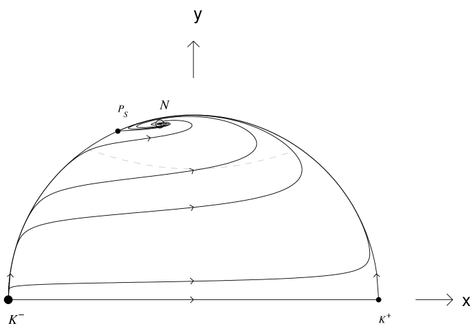
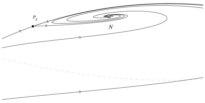
5.3 Case II: $\delta=a\mu H$: Perturbation Analysis

This section provides a second example to demonstrate that other types of interaction terms can lead to a similar behaviour; i.e., that there will be a range of parameters for which the inflationary models which drive the matter fields to zero are not late-time attractors, and for which the trajectories exhibit an oscillatory behaviour as they asymptote to the late-time attracting solution. Specifically, the interaction term $\delta=a\mu H$ is chosen, where $a>0$.

With this choice, equations (5.7a) become

$$x^{\prime} = -3x(1-x^{2})-\sqrt{\frac{3}{2}}ky^{2}+\left(\frac{3}{2}\gamma x-\frac{a}{2x}\right)\left(1-x^{2}-y^{2}\right),$$ (5.27a)

$$y^{\prime} = \frac{3}{2}y\left[\sqrt{\frac{2}{3}}kx+2x^{2}+\gamma(1-x^{2}-y^{2})\right].$$ (5.27b)

For physical reasons, the line $x=0$ will not be considered. Consequently, a full phase-plane analysis is not possible using these variables. However, it is still possible to determine the equilibrium points with $x\neq 0$ for the system and determine their local stability. Therefore, the analysis provided will constitute a perturbation analysis whereby the stability of equilibrium points cannot determine the global behaviour of the system.

There are four equilibrium points for this system for $x\neq 0$:

1. ${\cal K}^{+}:\qquad(x,y)=(+1,0),\qquad\Omega=0,\qquad q=2,$
   The eigenvalues for this equilibrium point are

   $$\left(\lambda_{1},\lambda_{2}\right)=\left(3[2-\gamma]+a,\sqrt{\frac{3}{2}}\sqrt{6}+3\right)$$ (5.28)

   This equilibrium point is a source.

2. ${\cal K}^{-}:\qquad(x,y)=(-1,0),\qquad\Omega=0,\qquad q=2.$
   The eigenvalues for this equilibrium point are

   $$\left(\lambda_{1},\lambda_{2}\right)=\left(3[2-\gamma]+a,-\sqrt{\frac{3}{2}}+3\right),$$ (5.29)

   and so ${\cal K}^{-}$ is a source for $k^{2}<6$ and a saddle otherwise.

3. $\displaystyle P_{\cal S}:\qquad(x,y)=\left(-\frac{k}{\sqrt{6}},\sqrt{1-\frac{k^{2}}{6}}\right),\qquad\Omega=0,\qquad q=\frac{1}{2}(k^{2}-2).$
   The eigenvalues for this equilibrium point are

   $$\left(\lambda_{1},\lambda_{2}\right)=\left(-\frac{1}{2}\left[6-k^{2}\right],-\left[\Xi-k^{2}\gamma-k^{2}\right]\right),$$ (5.30)

   where $\Xi\equiv 3\gamma-a$. This point exists only for $k^{2}<6$, and is a sink for $k^{2}<3\gamma$ and $a<3\gamma-k^{2}$ (saddle otherwise).

4. $\displaystyle{\cal N}_{1}:\qquad(x,y)=\left(-\frac{\Xi}{\sqrt{6}k},\sqrt{\frac{a}{3\gamma}+\frac{(2-\gamma)}{\gamma}\frac{\Xi^{2}}{6k^{2}}}\right),\qquad\Omega=\frac{\Xi(k^{2}-\Xi)}{3\gamma k^{2}},$
   $\displaystyle q=-1+\frac{1}{2}\Xi,$             
   Note that this solution is physical ($\Omega\geq 0)$ for $[3\gamma-k^{2}]<a<3\gamma$ and $k^{2}<3\gamma$, and represents an inflationary model for $a>(3\gamma-2)$ (consequently, this model will always inflate for $k^{2}<2$ and can inflate for $2<k^{2}<3\gamma$). The eigenvalues for this equilibrium point are

   $$\lambda_{\pm} = -\frac{[2a(2\Xi-k^{2})+(2-\gamma)\Xi^{2}]}{4\gamma\Xi}$$

   $$\pm\frac{\sqrt{\left[2a(2\Xi-k^{2})+(2-\gamma)\Xi^{2}\right]^{2}k^{2}-8\gamma\Xi^{2}(k^{2}-\Xi)\left[2ak^{2}+(2-\gamma)\Xi\right]}}{4\gamma\Delta k},$$

   and so ${\cal N}_{1}$ is a sink for $a<3\gamma-\frac{1}{2}k^{2}$. Note that the scalar field acts as a perfect fluid with an equation of state parameter given by

   $$\gamma_{\phi}=\frac{\gamma}{1+\frac{ak^{2}}{\Xi^{2}}}<\gamma.$$ (5.32)

Table 5.3 lists the equilibrium points and their stability for the ranges of $k$ and $a$.

	$0<k^{2}<2$			$2<k^{2}<3\gamma$			$3\gamma<k^{2}<6$
	$a<G_{3}$	$a>G_{3}$		$a<G_{3}$	$a>G_{3}$
		$a<G_{4}$	$a>G_{4}$		$a<G_{4}$	$a>G_{4}$
${\cal K}^{\pm}$	R
	(NI)
$P_{\cal S}$	A	s		A	s
	(I)	(I)		(NI)	(NI)
${\cal N}_{1}$		A	s		A	s
	$-$	(I)	(I)	$-$	(I) for	(I) for	$-$
					$a>3\gamma-2$	$a>3\gamma-2$

Table 5.3: The equilibrium points for the model with $\delta=a\mu H$ and their stability for various values of $k$ and $a$. Note that $G_{3}\equiv 3\gamma-k^{2}$ and $G_{4}\equiv 3\gamma-\frac{1}{2}k^{2}$. The symbol “R” denotes when the equilibrium point is a source (repellor), “s” for when it is a saddle, “A” for when it is a sink (attractor), and “$-$” when it does not exist within the particular parameter space. The label “(NI)” denotes non-inflationary models whereas “(I)” represents inflationary models. For $k^{2}>6$ the only equilibrium points to exist are the points ${\cal K}^{\pm}$, for which ${\cal K}^{+}$ is a source and ${\cal K}^{-}$ is a saddle.

Again, for the range $k^{2}<2$ and $(3\gamma-\frac{1}{2}k^{2})<a<(3\gamma-\frac{1}{2}k^{2})$, the power-law model $P_{\cal S}$ is no longer a sink and ${\cal N}_{1}$ is a sink. Therefore, solutions approach the equilibrium point which is represented by $P_{\cal S}$ (thereby inflating) for an indefinite period of time, but eventually evolve away. It can be shown numerically that within this range for $k$ and $a$, the equilibrium point ${\cal N}_{1}$ is a spiral node (for instance, for $k=1$ and $\gamma=4/3$, ${\cal N}_{1}$ is a sink for $3<a<3.5$ and a spiral sink for $3.24\lesssim a<3.5$); therefore the scalar field exhibits oscillatory motion as the solutions asymptotes to ${\cal N}$.

5.4 Discussion

Without an interaction term, it is known that for $k^{2}<2$ the late-time attractor for the system (5.7a) is a power-law inflationary model in which the matter is driven to zero [60]. The purpose of this chapter was to determine whether this behaviour could be altered qualitatively with the introduction of an interaction term. Two examples given have show that this is indeed possible. In particular, there are values in the parameter space for which this particular power-law inflationary model becomes a saddle point, and so while the models may spend an indefinite period of time inflating with $\Omega\rightarrow 0$, they eventually evolve away from this solution. The late-time attractors within the same parameter space are also inflationary, however the matter field’s energy density remains a fixed fraction of the scalar field’s energy density and indeed to the total energy density.

In the absence of an interaction term, matter scaling solutions are represented by equilibrium points of the dynamical system. It was shown here that for simple models found in the literature, they cannot be represented by equilibrium points when an interaction term is introduced. However, new equilibrium points can arise which represent models in which the energy densities of the matter and scalar field remain a fixed proportion to one another. Indeed, these models are equivalent to a two-perfect-fluid model (for an example of two-perfect-fluid model see [160]); for the examples given, the constant $\gamma_{\phi}$ for the scalar field was given, obeying $\gamma_{\phi}<\gamma$. The solutions corresponding to these equilibrium points are analogues of the matter scaling solutions in which $\gamma_{\phi}=\gamma$.

In the first example ($\delta=-a\dot{\phi}\mu$) a phase-plane analysis was performed to determine the qualitative properties and detailed calculations for particular values $k=1$ and $\gamma=4/3$ (radiation) were used to describe the qualitative behaviour described in more detail (see figure 5.1). In the second example ($\delta=a\mu H$), the system as described is not well behaved for $x=0$ and so only the local behaviour of the relevent equilibrium points is discussed. Again, the power-law inflationary model, represented by $P_{\cal S}$, becomes a saddle point and the only attracting equilibrium point is ${\cal N}_{1}$.

For an appropriate parameter range, the equilibrium point ${\cal N}_{1}$ is an attracting focus, and hence as solutions approach this late-time attractor the scalar field oscillates. Although the late-time behaviour is still inflationary, the oscillatory behaviour provides a possible mechanism for inflation to stop and for conventional reheating to ensue (indeed this is similar to the mechanism for reheating in scalar field models with a potential containing a global minimum [24, 28, 143, 145, 147]). To study reheating properly more complicated physics in which the oscillating scalar field is coupled to both fermionic and bosonic fields needs to be included. This contrasts with the situation for exponential models for $k^{2}<2$ with no interaction term which have no graceful exit from inflation and in which there is no conventional reheating mechanism.

Therefore, it has been shown that there are general relativistic scalar field models with an exponential potential which evolve towards an inflationary state in which the matter is not driven to zero and which exhibit late-time oscillatory behaviour; these models may constitute a first step towards a more realistic model. There is the question of how physical these models are, since they correspond to relatively large values of $a$. In the context that the interaction term represents energy transfer, for physical reasons it might be expected that $a$ must be small; i.e., $a<0.1$ [63] (see also [161]). On the other hand, in the context of scalar-tensor theories $a$ is of order unity and can certainly attain values large enough to produce the behaviour described above; this is also the situation in the context of string theories.

It is also of interest to study the cosmological consequences of the ‘decaying cosmological constant’ or ‘quintessential’ cosmological models, since they may be consistent with the observations of accelerated expansion [162, 163] and may lead to a physically interesting residual scalar field energy-density which is still present today. These issues have recently been addressed by Amendola [164, 165] in the context of the conformally related scalar-tensor theories of gravity.

Finally, it is worth noting that inflationary solutions can be obtained when $k^{2}>2$, unlike the case in which there is no interaction term. Moreover, from Table 5.2 it can be seen that these inflationary solutions occur for $a>\frac{1}{2}(3\gamma-2)k$ and are sinks (attractors). This result complements the results of [59, 157] who looked for inflationary solutions for steeper potentials. When $k^{2}<2$ and $0<a<(3\gamma-k^{2})/2$ the power-law inflationary solution corresponding to the equilibrium point $P_{\cal S}$ is again a global attracting solution. The late-time behaviour of these models, both inflationary and non-inflationary, may also be of cosmological interest. Due to recent observations of accelerated expansion [162, 163], models that are presently inflating are also of interest.

Chapter 6 String Models I: Non-Zero Central Charge Deficit

The next four chapters consider string models defined by action (1.28) in the Introduction. The general solutions to the field equations of action (1.28) are known analytically when $\Lambda=\Lambda_{\rm M}=Q=0$ for both the spatially flat and isotropic Friedmann–Robertson–Walker (FRW) universes and the anisotropic Bianchi type I models [129, 166, 167]. It can be shown that the action (1.28) is invariant under a global ${\rm SL}(2,R)$ transformation on the dilaton and axion fields [168, 169], when $\Lambda=\Lambda_{\rm M}=Q=0$. The general Friedmann–Robertson–Walker (FRW) cosmologies derived from equation (1.28) (with $\Lambda=\Lambda_{\rm M}=Q=0$) have been found by employing this symmetry [129, 166]. Specifically, the general solution where only $\Lambda=\Lambda_{\rm M}=Q=0$ is the ‘dilaton–moduli–axion’ solution [129, 166] (see equation (6.8) for $d=0$). This cosmology asymptotically approaches one of the dilaton–moduli–vacuum solutions (see (6.7) for $h_{0}^{2}=\frac{1}{3}$) in the limits of high and low spacetime curvature. The axion field induces a smooth transition between these two power-law solutions and causes a bounce to occur. It is only dynamically important for a short time interval when $s\approx s_{0}$ [129, 166]. However, the ${\rm SL}(2,R)$ symmetry is broken when a cosmological constant is present [170] (either $\Lambda$, $\Lambda_{\rm M}$ or $Q$) and the general FRW solution is not known in this case. There are two known solutions, which are the “rolling radii” solutions found by Mueller [171, 172, 173, 174, 175] (see equation (6.11)), and the “linear dilaton-vacuum” solution [176, 177, 178] (see equation (6.12)). Previously, analytical solutions had not been found for this model when the axion field is trivial and $\Lambda_{\rm M}>0$ [78, 179]. Moreover, the combined effects of $\Lambda_{\rm M}$ and axion field had not been considered previously. The work herein extends previous qualitative analyses where one or more of the terms in action (1.28) was neglected [180, 181, 182, 183, 184, 185].

As will be demonstrated, most of the analysis to follow is equally applicable to curved FRW models with a modulus field and to certain Bianchi type I, V and IX models with or without a modulus field, and therefore extends the work by Easter et al. [182], who performed a perturbation analysis to a static $k=+1$ FRW solution to show that it was a late-time attractor. The only section where this equivalence does not hold is in chapters 8 and 9 wherein only curved FRW models are considered (the shear terms have been neglected).

In this chapter, $\Lambda_{\rm M}=0$ and $Q=0$ in order to determine the rôle of $\Lambda$ in the dynamics of the system (6.5a), although several comments here are equally applicable to the following chapters. The chapter is organized as follows. In section 6.1, the field equations with all parameters present are derived from the string action. All of the terms of action (1.28) will be kept arbitrary for this section so that they can be used in subsequent chapters, but $\Lambda_{\rm M}=Q=0$ will be used for the actual analysis of this chapter. All the known corresponding exact solutions are listed in section 6.2 for $\Lambda_{\rm M}=Q=0$. Section 6.3 discusses the asymptotic behaviour of the axion and curvature terms. There it will be shown that for most cases either one of the two will asymptotically dominate at early or late times, and hence the four-dimensional dynamical system can be reduced to a three-dimensional system. The arguments in this section are equally applicable to the analysis of chapter 7. For the remainder of the chapter, the case $\Lambda_{\rm M}=Q=0$ is explicitly studied, examining the combined effects of the axion field, modulus field and central charge, thereby extending previous qualitative analyses [180, 181, 182, 183, 184, 185]. The chapter ends with a summary section and a section which discusses the corresponding solutions and asymptotic behaviour in the Einstein frame. Since the work in this chapter is primarily confined to the Jordan frame, the index “(st)” shall be omitted to save notation, but must be introduced again in the final section when both frames are discussed.

6.1 Governing Equations

A class of spatially-homogeneous spacetimes with non-trivial curvature shall be considered here. It shall assumed that the three-dimensional Ricci curvature tensor is isotropic; i.e., ${}^{3}R_{\mu\nu}$ is proportional to $k\delta_{\mu\nu}$ on the spatial hypersurfaces (and hence the spatial hypersurfaces have constant curvature $k$) [186]. This class of models, more commonly known as the isotropic curvature models, contain the Bianchi type I ($k=0$) and V ($k<0$) models and a special case of the Bianchi type IX ($k>0$) model. In essence, these isotropic curvature models can be regarded as the simplest anisotropic generalizations of FRW (flat, open, closed, respectively) models.

In particular, the four–dimensional, anisotropic, space–time with constant curvature $k$ shall be assumed, with a line element of the form

$$ds^{2}=-dt^{2}+e^{2\alpha(t)}\left[\left(\mathbf{\omega}^{1}\right)+e^{-2\sqrt{3}\beta_{s}(t)}\left(\mathbf{\omega}^{2}\right)^{2}+e^{2\sqrt{3}\beta_{s}(t)}\left(\mathbf{\omega}^{3}\right)^{2}\right],$$ (6.1)

where

for $$k=0 [\mathbf{\omega}^{1},\mathbf{\omega}^{2},\mathbf{\omega}^{3}]=\left[dx,dy,dz\right]$$ (Bianchi I) (6.2a)

for $$k<0 [\mathbf{\omega}^{1},\mathbf{\omega}^{2},\mathbf{\omega}^{3}]=\left[dx,e^{x}dy,e^{x}dz\right]$$ (Bianchi V) (6.2b)

for $$k>0 [\mathbf{\omega}^{1},\mathbf{\omega}^{2},\mathbf{\omega}^{3}]=\left[dx-\sin y\,dz,\right.$$ (Bianchi IX) (6.2c)

$$\qquad\qquad\qquad\cos x\,dy+\cos y\,\sin x\,dz,$$

$$\left.\qquad\qquad\qquad-\sin x\,dy+\cos y\,\cos x\,dz\right].$$

Since, the modulus field ($\beta_{m}$) has the same functional form in the field equations as the shear terms ($\beta_{s}$) when $Q=0$, both terms can be combined via

$${\dot{\beta}}^{2}\equiv{\dot{\beta}}_{s}^{2}+{\dot{\beta}}_{m}^{2},$$ (6.3)

to yield the same field equations. Indeed, several modulus fields can be included via

$${\dot{\beta}}^{2}={\dot{\beta}}_{s}^{2}+\Sigma{\dot{\beta}}_{m}^{2}.$$ (6.4)

It shall be implicit throughout the text that the appearance of the “$\beta$” term is the combination of the shear and modulus field for the $Q=0$ cases, but will only represent $\beta_{m}$ when $Q\neq 0$ (when $Q\neq 0$, only flat FRW models will be considered and hence there will be no shear terms).

The field equations derived from the action (1.28) are then given by

$$\ddot{\alpha}-\dot{\alpha}\dot{\varphi}-\frac{1}{2}\rho+\tilde{K}+\frac{1}{2}\Lambda_{\rm M}e^{\varphi+3\alpha}+\frac{1}{4}Q^{2}e^{-6\beta+\varphi+3\alpha}=0,$$ (6.5a)

$$2\ddot{\varphi}-\dot{\varphi}^{2}-3\dot{\alpha}^{2}-6\dot{\beta}^{2}+\frac{1}{2}\rho-3\tilde{K}+2\Lambda=0,$$ (6.5b)

$$\ddot{\beta}-\dot{\beta}\dot{\varphi}-\frac{1}{4}Q^{2}e^{-6\beta+\varphi+3\alpha}=0,$$ (6.5c)

$$\dot{\tilde{K}}+2\dot{\alpha}\tilde{K}=0,$$ (6.5d)

$$\dot{\rho}+6\dot{\alpha}\rho=0,$$ (6.5e)

together with the generalized Friedmann constraint equation

$$3\dot{\alpha}^{2}-\dot{\varphi}^{2}+6\dot{\beta}^{2}+\frac{1}{2}\rho-3\tilde{K}+2\Lambda+\Lambda_{\rm M}e^{\varphi+3\alpha}+\frac{1}{2}Q^{2}e^{-6\beta+\varphi+3\alpha}=0,$$ (6.6)

where $\varphi\equiv\hat{\Phi}-3\alpha$ defines the ‘shifted’ dilaton field, $\tilde{K}\equiv 2k\exp(-2\alpha)$ represents the curvature term, $\rho\equiv\dot{\sigma}^{2}\exp(2\varphi+6\alpha)>0$ may be interpreted as the effective energy density of the pseudo–scalar axion field, $\beta$ is defined by (6.3), and a dot denotes differentiation with respect to cosmic time, $t$.

6.2 Exact Solutions

The exact solutions that were either quoted or defined in [104] and [105] are here listed.

The dilaton–moduli–vacuum solutions, which are found in all sectors (and therefore $\Lambda=\Lambda_{\rm M}=Q=0$), are given by

$$a = a_{0}\left|t\right|^{\pm h_{0}},$$

$$e^{\hat{\Phi}} = e^{\hat{\Phi}_{0}}\left|t\right|^{\pm 3h_{0}-1},$$

$$e^{\beta} = e^{\beta_{0}}\left|t\right|^{\pm\epsilon\sqrt{(1-3h_{0}^{2})/6}},$$

$$\sigma = \sigma_{0},$$

$$k = 0,$$ (6.7)

where $\{\hat{\Phi}_{0},\sigma_{0},\beta_{0},h_{0}\}$ are constants, $a$ is the scale factor ($a\equiv e^{\alpha}$), the $\pm$ sign corresponds to the sign of $t$ (note that $\dot{\varphi}>0$ for $t<0$ and $\dot{\varphi}<0$ for $t>0$) and $\epsilon=\pm 1$. The “$+$” solution for $h_{0}=\pm\frac{1}{3}$ corresponds to the $\dot{\beta}=0$ equilibrium points $L^{-}_{(\pm)}$ throughout this chapter and the “$-$” solution for $h_{0}=\pm\frac{1}{3}$ correspond to the equilibrium points $L^{+}_{(\pm)}$. Because the modulus field is static for these four end-points, they are referred to only as dilaton–vacuum solutions. For $t<0$ (i.e. $L^{+}$) these solutions are inflationary (i.e., $H>0$, $q<0$) for $h_{0}>0$.

These exact solutions are a subset to the dilaton-moduli-axion solutions:

$$a = a_{0}\left|\frac{s}{s_{0}}\right|^{\frac{1}{2}}\left[\left|\frac{s}{s_{0}}\right|^{c}+\left|\frac{s}{s_{0}}\right|^{-c}\right]^{\frac{1}{2}},$$

$$e^{\hat{\Phi}} = \frac{e^{\hat{\Phi}_{0}}}{2}\left[\left|\frac{s}{s_{0}}\right|^{c}+\left|\frac{s}{s_{0}}\right|^{-c}\right],$$

$$e^{\beta} = e^{\beta_{0}}\left|\frac{s}{s_{0}}\right|^{d},$$

$$\sigma = \sigma_{0}\pm e^{-\hat{\Phi}_{0}}\left[\frac{|\frac{s}{s_{0}}|^{-c}-|\frac{s}{s_{0}}|^{c}}{|\frac{s}{s_{0}}|^{-c}+|\frac{s}{s_{0}}|^{c}}\right],$$

$$k = 0,$$ (6.8)

where $\{a_{0},\hat{\Phi}_{0},\beta_{0},\sigma_{0}\}$ are an arbitrary constants, $c\equiv|\sqrt{3-12d^{2}}|$, and $s\!\equiv\!\int^{t}dt^{\prime}/a(t^{\prime})$.

Another solution which appears in both the NS-NS and matter sectors ($\Lambda=\Lambda_{\rm M}=0$) but not in the R–R sector ($Q\neq 0$) is the saddle-point Milne solution [13, p. 205] (i.e. Minkowski space):

$$a = a_{0}\left(\pm t\right),$$

$$\hat{\Phi} = \hat{\Phi}_{0},$$

$$\beta = \beta_{0},$$

$$\sigma = \sigma_{0},$$

$$k = -a_{0}^{2},$$ (6.9)

where $\{a_{0},\hat{\Phi}_{0},\beta_{0},\sigma_{0}\}$ are constants. The “$\pm$” sign corresponds to the sign of $t$. These solutions are represented by the equilibrium points denoted by $S^{\mp}$ throughout this chapter.

The ten-dimensional isotropic, frozen axion solution is given by

$$a = a_{0}\left|{\rm tanh}(\frac{1}{2}At)\right|^{\pm\frac{1}{3}},$$

$$e^{-\hat{\Phi}} = e^{-\hat{\Phi}_{0}}\left|\cosh(\frac{1}{2}At)\right|^{(1\pm 3)}\left|\sinh(\frac{1}{2}At)\right|^{(1\mp 3)},$$

$$e^{\beta} = e^{\beta_{0}}\left|{\rm tanh}(\frac{1}{2}At)\right|^{\pm\frac{1}{3}},$$

$$\sigma = \sigma_{0},$$

$$k = 0,$$ (6.10)

where $A\equiv\sqrt{2\Lambda}$ and $\{a_{0},\hat{\Phi}_{0},\beta_{0},\sigma_{0}\}$ are constants. The generalization of this solution is the “rolling radii” solutions:

$$a = a_{0}\left|{\rm tanh}(\frac{1}{2}At)\right|^{m},$$

$$e^{-\hat{\Phi}} = e^{-\hat{\Phi}_{0}}\left|\cosh(\frac{1}{2}At)\right|^{2p-6n}\left|\sinh(\frac{1}{2}At)\right|^{2l+6n},$$

$$e^{\beta} = e^{\beta_{0}}\left|{\rm tanh}(\frac{1}{2}At)\right|^{6n},$$

$$\sigma = \sigma_{0},$$

$$k = 0,$$ (6.11)

where $A\equiv\sqrt{2\Lambda}$ and the real numbers $\{l,m,n,p\}$ satisfy

$$3m^{2}+6n^{2}=1,\qquad 3m+6n=p-l,\qquad p+l=1.$$

The corresponding solutions for $\Lambda<0$ are related to (6.11) by redefining $A\equiv-i\sqrt{2\Lambda}$. In this case, the range of $t$ is bounded such that $0<t<\pi/A$.

The static ‘linear dilaton–vacuum’ solution [176, 177, 178] is given by

$$a = a_{0},$$

$$\hat{\Phi} = \hat{\Phi}_{0}\pm\sqrt{2\Lambda}t,$$

$$\beta = \beta_{0},$$

$$\sigma = \sigma_{0},$$

$$k = 0,$$ (6.12)

where $\{a_{0},\hat{\Phi}_{0},\beta_{0},\sigma_{0}\}$ are constants. This solution is represented by the equilibrium points $C^{\pm}$, where “$\pm$” corresponds to the “$\pm$” sign in (6.12).

This solution had been generalized in [96] to the ‘generalized linear dilaton–vacuum’, to include the axion field and a curvature term:

$$a = a_{0},$$

$$\hat{\Phi} = \hat{\Phi}_{0}+n\sqrt{\frac{6\Lambda}{2+n^{2}}}t,$$

$$\beta = \beta_{0},$$

$$\sigma = \sigma_{0}\pm\sqrt{\frac{2\left(1-n^{2}\right)}{3n^{2}}}\exp\left(-\hat{\Phi}_{0}-n\sqrt{\frac{6\Lambda}{2+n^{2}}}t\right),$$

$$k = \frac{1-n^{2}}{2+n^{2}}\Lambda a_{0}^{2},$$ (6.13)

where $n\in[-1,1]$. The solutions are represented by the line of equilibrium points denoted throughout this chapter by $L_{1}$. Note that $C^{\pm}=L_{1}$ when $n^{2}=1$ ($\rho=k=0$).

6.3 Asymptotic Behaviour

Returning to the field equations (6.5a) and (6.6), the variables $\rho$ and $\tilde{K}$ may be combined to define the new variable

$$\Xi\equiv\frac{\rho-\tilde{K}}{\rho+\tilde{K}},$$ (6.14)

and hence (6.5d) and (6.5e) can be combined to yield the evolution equation

$$\dot{\Xi}=-2\dot{\alpha}\left(1-\Xi^{2}\right).$$ (6.15)

Hence, all of the equilibrium sets occur either for $\dot{\alpha}=0$ or for $\Xi^{2}=1$, and therefore if $\dot{\alpha}\neq 0$ then either $\rho=0$ ($\Xi=-1$) or $\tilde{K}=0$ ($\Xi=+1$) asymptotically. Equations (6.5a) and (6.6) define a four-dimensional dynamical system (although there are five ODE’s, equation (6.6) can be used to globally reduce the system by one dimension). In the cases in which all of the equilibrium sets lie on $\Xi^{2}=1$, the asymptotic properties of the string cosmologies can be determined from the dynamics in the three-dimensional sets $\rho=0$ or $\tilde{K}=0$.

In what follows, the three-dimensional $\rho=0$ case and $\tilde{K}=0$ case will be consequently explicitly examined separately. The only case in which there exist equilibrium sets with $\dot{\alpha}=0$ but $\Xi^{2}\neq 1$ occurs in the NS-NS case ($\Lambda_{\rm M}=Q=0$) in which $\tilde{K}>0$ and $\Lambda>0$, and therefore the full four-dimensional system shall be examined in this case, although the three-dimensional subset $\rho=0$ still plays a principal rôle in the asymptotic analysis.

6.4 Analysis

In this chapter, $\Lambda_{\rm M}=0$ and $Q=0$ in order to determine the rôle of $\Lambda$ in the dynamics of the system (6.5a). Through equation (6.6), the variable $\rho$ is eliminated from the field equations, and the following definitions are made:

$$X\equiv\frac{\sqrt{3}\dot{\alpha}}{\xi},\quad Y\equiv\frac{\dot{\varphi}}{\xi},\quad Z\equiv\frac{6\dot{\beta}^{2}}{\xi^{2}},\quad U\equiv\frac{\pm 3\tilde{K}}{\xi^{2}},\quad V\equiv\frac{\pm 2\Lambda}{\xi^{2}},\quad\frac{d}{dt}\equiv\xi\frac{d}{dT},$$ (6.16)

where the $\pm$ sign in the definitions for $U$ and $V$ are to ensure $U>0$ and $V>0$, where necessary. With these definitions, all variables are bounded: $0\leq\{X^{2},Y^{2},Z,U,V\}\leq 1$. Equation (6.6) now reads

$$\kappa=Y^{2}\pm U\mp V-X^{2}-Z\geq 0,$$ (6.17)

where

$$\kappa\equiv\frac{1}{2}\frac{\rho}{\xi^{2}}$$ (6.18)

The variable $\xi$ is defined in each of the following six cases by:

• $\Lambda>0$

  • $\tilde{K}>0$: $\xi^{2}\equiv 3\tilde{K}+\dot{\varphi}^{2}$ (subsection 6.4.2),

  • $\tilde{K}\leq 0$: $\xi^{2}\equiv\dot{\varphi}^{2}$ (subsections 6.4.1 and 6.4.3),

• $\Lambda<0$

  • $\tilde{K}>0$: $\xi^{2}\equiv 3\tilde{K}+\dot{\varphi}^{2}-2\Lambda$ (subsection 6.4.2),

  • $\tilde{K}\leq 0$: $\xi^{2}\equiv\dot{\varphi}^{2}-2\Lambda$ (subsections 6.4.4 and 6.4.6).

For example, consider $\Lambda>0$ with $\tilde{K}>0$; for this case $Y^{2}+U=1$ and equation (6.17) reads

$$\kappa=1-V-X^{2}-Z\geq 0.$$ (6.19)

Hence the variables $\{X,V,Z\}$ will be used as the phase space variables (see section 6.4.2 for details). The only exception to this approach is the $\tilde{K}=0$ cases in sections 6.4.1 and 6.4.4 in which $\dot{\beta}$ is removed from the field equations in lieu of $\rho$. Although this deviation from the orthodox of the other sections was performed merely to give an example where the axion field explicitly remains in the dynamics, it leads to the exact qualitative behaviour if $\dot{\beta}$ had been kept and not $\rho$.

Each of six cases will now be considered. Subscripts will be added to the variables $\{X,Y,Z,U,V\}$ to indicate each case, although the $\tilde{K}=0$ cases will have the same subscript as the $\tilde{K}>0$ (for either $\tilde{K}>0$ or $\tilde{K}<0$, the phase space variables reduce to the same form when $\tilde{K}=0$ and so the notation is consistent with either case; however, since the $\tilde{K}>0$ case follows the $\tilde{K}=0$ in what follows, the above subscript choice will be made). In each of the following subsections, the four-dimensional dynamical systems for $\tilde{K}\neq 0$ will be established, and the $\rho=0$ invariant set will be examined. As discussed in section 6.3, all equilibrium sets discussed below which have $\dot{\alpha}=0$ also have $\Xi\neq 1$, and hence nearly all orbits asymptote towards the equilibrium sets in one of the invariant sets $\rho=0$ or $\tilde{K}=0$, where the three-dimensional $\tilde{K}=0$ case will be studied in its own subsection. The qualitative behaviour of the full four-dimensional phase space in each $\tilde{K}\neq 0$ case will also be examined.

6.4.1 The Case $\Lambda>0$, $\tilde{K}=0$

For this case, it proves convenient to employ the generalized Friedmann constraint equation (6.6) to eliminate the modulus field rather than the axion field, and the definition $\xi^{2}=\dot{\varphi}^{2}$ is used. From the generalized Friedmann equation one has that

$$0\leq X_{1}^{2}+\kappa+Z_{1}\leq 1,$$ (6.20)

and equations (6.5a) and (6.6) transform to the three–dimensional autonomous system:

$$\frac{dX_{1}}{dT} = \kappa+\frac{X_{1}}{\sqrt{3}}\left[1-X_{1}^{2}-Z_{1}\right],$$ (6.21a)

$$\frac{d\kappa}{dT} = -2\kappa\left[X_{1}+\frac{1}{\sqrt{3}}\left(Z_{1}+X_{1}^{2}\right)\right],$$ (6.21b)

$$\frac{dZ_{1}}{dT} = \frac{2}{\sqrt{3}}Z_{1}\left(1-X_{1}^{2}-Z_{1}\right).$$ (6.21c)

The sets $\kappa=0$ and $Z_{1}=0$ are invariant sets corresponding to $\rho=0$ and $\dot{\beta}=0$, respectively. In addition, $X_{1}^{2}+\kappa+Z_{1}=1$ is an invariant set corresponding to $\Lambda=0$. Note that the right-hand side of equation (6.21c) is positive-definite and this simplifies the dynamics considerably.

The Frozen Modulus ($\dot{\beta}=0$) Invariant Set

It is also instructive to first consider the dynamics on the boundary corresponding to $Z_{1}=0$, since the case $\dot{\beta}=0$ is of physical interest in its own right as a four–dimensional model. Here the dynamical system becomes equations (6.21a) and (6.21b) with $Z_{1}=0$, and the equilibrium points (and their eigenvalues) are given by

$$C^{+}: X_{1}=\kappa=0;$$ (6.22a)

$$(\lambda_{1},\lambda_{2})=\left(\frac{1}{\sqrt{3}},0\right),$$

$$L^{+}_{(-)}: X_{1}=-1,\kappa=0;$$ (6.22b)

$$(\lambda_{1},\lambda_{2})=\left(-2\left[-1+\frac{1}{\sqrt{3}}\right],-\frac{2}{\sqrt{3}}\right),$$

$$L^{+}_{(+)}: X_{1}=+1,\kappa=0;$$ (6.22c)

$$(\lambda_{1},\lambda_{2})=\left(-2\left[1+\frac{1}{\sqrt{3}}\right],-\frac{2}{\sqrt{3}}\right)$$

(throughout these chapters, the corresponding eigenvectors will not be explicitly given). Point $C^{+}$ is a non-hyperbolic equilibrium point; however, by changing to polar coordinates $C^{+}$ can be shown to be a repeller with an invariant ray $\theta=\tan^{-1}(-\sqrt{3})$. The phase portrait is given in figure 6.1.

Figure 6.1: Phase diagram of the system (6.21a) in the NS-NS ($\Lambda>0$) sector with $\tilde{K}=\dot{\beta}=0$. In this phase space, $\dot{\varphi}>0$ is assumed. Equilibrium sets are denoted by dots and the labels in all figures correspond to those equilibrium sets (and hence the exact solutions they represent) discussed in the text. The convention adopted throughout will be that large black dots represent sources (i.e., repellors), large grey-filled dots represent sinks (i.e., attractors), and small black dots represent saddles. Arrows on the trajectories denote the direction of increasing time.

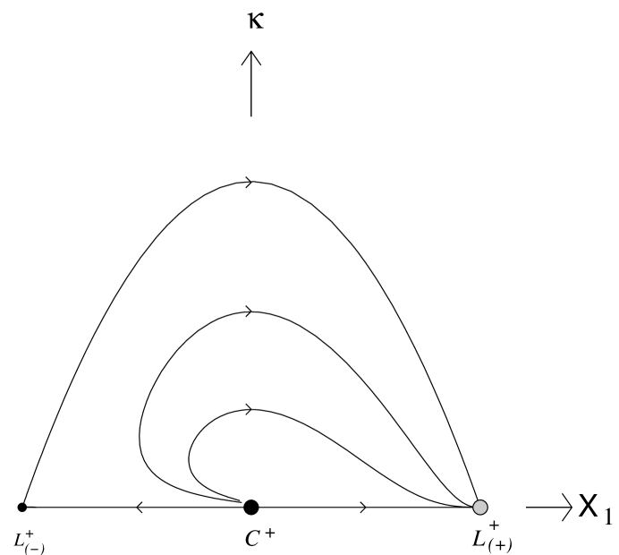
Three–Dimensional System ($\dot{\beta}\neq 0$)

Returning to the full three-dimensional dynamical system (6.21a), the equilibrium sets of the system (and their corresponding eigenvalues) are

$$C^{+}: X_{1}=\kappa=Z_{1}=0;$$ (6.23a)

$$(\lambda_{1},\lambda_{2},\lambda_{3})=\left(\frac{1}{\sqrt{3}},\frac{2}{\sqrt{3}},0\right),$$

$$L^{+}: X_{1}^{2}+Z_{1}=1,\kappa=0;$$ (6.23b)

$$(\lambda_{1},\lambda_{2},\lambda_{3})=\left(-2\left[X_{1}+\frac{1}{\sqrt{3}}\right],-\frac{2}{\sqrt{3}},0\right).$$

Although $C^{+}$ is non-hyperbolic, a simple analysis shows that it is a global source. Equilibrium points on $L^{+}$ are saddles for $X_{1}<-\frac{1}{\sqrt{3}}$ and local sinks for $X_{1}>-\frac{1}{\sqrt{3}}$. Note that the points $L^{+}_{(-)}$ and $L^{+}_{(+)}$ in the two–dimensional invariant set $\dot{\beta}=0$ are the endpoints to the line $L^{+}$. The phase space is depicted in figure 6.2.

The set $C^{+}$ represents the linear dilaton–vacuum solution (6.12) from which all solutions asymptote away. The line $L^{+}$ represents the dilaton–moduli–vacuum solutions (6.7) (the “$-$” branch) towards which all solutions asymptote into the future.

Figure 6.2: Phase diagram of the system (6.21a) in the NS-NS ($\Lambda>0$) sector with $\rho\neq 0$ and $\tilde{K}=0$. Note that $L^{+}$ represents a line of equilibrium points. In this phase space, $\dot{\varphi}>0$ is assumed. The invariant set $Z_{1}=0$ corresponds to the phase portrait 6.1. Dashed black lines are those trajectories along the intersection of the invariant sets, and solid black lines are typical trajectories within the full three-dimensional phase space. See also caption to figure 6.1 on page 6.1.

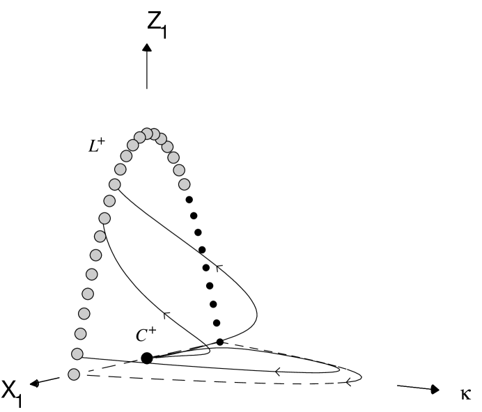
6.4.2 The Case $\Lambda>0$, $\tilde{K}>0$

In this case the choice $\xi^{2}=\dot{\varphi}^{2}+3\tilde{K}$ is made and the positive signs for $U_{1}$ and $V_{1}$ has been utilized, as defined by (6.16). The generalized Friedmann equation yields

$$0\leq X_{1}^{2}+Z_{1}+V_{1}\leq 1,\qquad Y_{1}^{2}+U_{1}=1,$$ (6.24)

and therefore $U_{1}$ (which is proportional to $\tilde{K}$) may be eliminated, yielding the four-dimensional system of ODEs for $0\leq\{X_{1}^{2},Y_{1}^{2},Z_{1},V_{1}\}\leq 1$:

$$\frac{dX_{1}}{dT} = \frac{1}{\sqrt{3}}\left(1-X_{1}^{2}\right)\left(2+Y_{1}^{2}\right)-\sqrt{3}\left(Z_{1}+V_{1}\right)+X_{1}Y_{1}\left(1\!-\!X_{1}^{2}\!-\!Z_{1}\right)\!\!,$$ (6.25a)

$$\frac{dY_{1}}{dT} = \left(1-Y_{1}^{2}\right)\left(X_{1}^{2}+Z_{1}+\frac{1}{\sqrt{3}}X_{1}Y_{1}\right),$$ (6.25b)

$$\frac{dZ_{1}}{dT} = 2Z_{1}\left[Y_{1}\left(1-X_{1}^{2}-Z_{1}\right)+\frac{1}{\sqrt{3}}X_{1}\left(1-Y_{1}^{2}\right)\right],$$ (6.25c)

$$\frac{dV_{1}}{dT} = -2V_{1}\left[Y_{1}\left(X_{1}^{2}+Z_{1}\right)-\frac{1}{\sqrt{3}}X_{1}\left(1-Y_{1}^{2}\right)\right].$$ (6.25d)

The invariant sets $Y_{1}^{2}=1$, $X_{1}^{2}+Z_{1}+V_{1}=1$, $Z_{1}=0$ and $V_{1}=0$ define the boundary of the phase space. The equilibrium sets and their corresponding eigenvalues (denoted by $\lambda$) are

$$L^{\pm}: Y_{1}=\pm 1,Z_{1}=1-X_{1}^{2},V_{1}=0;$$ (6.26a)

$$\left(\lambda_{1},\lambda_{2},\lambda_{3},\lambda_{4}\right)=\left(\mp\frac{2}{\sqrt{3}}\left[\sqrt{3}\pm X_{1}\right],\mp 2,0,-2\sqrt{3}\left[X_{1}\pm\frac{1}{\sqrt{3}}\right]\right),$$

$$L_{1}: X_{1}=0,Z_{1}=0,V_{1}=\frac{1}{3}(2+Y_{1}^{2});$$ (6.26b)

$$\left(\lambda_{\pm},\lambda_{2},\lambda_{3}\right)=\left(\frac{1}{2}\left[Y_{1}\pm\frac{1}{\sqrt{3}}\sqrt{19Y_{1}^{2}-16}\right],2Y_{1},0\right).$$

The zero eigenvalue in each arise because these are all lines of equilibrium points. Here, the global sources are the lines $L_{1}$ (for $Y_{1}>0$ or $\dot{\varphi}>0$) and $L^{-}$ (for $X_{1}<\frac{1}{\sqrt{3}}$). The global sinks are the lines $L_{1}$ (for $Y_{1}<0$) and $L^{+}$ (for $X_{1}>-\frac{1}{\sqrt{3}}$).

This case is different from the other cases to be considered, since it is the only one with the line of equilibrium points, $L_{1}$, inside the phase space and this line acts as both sink and source (all the other cases, as will be shown, have equilibrium points only on the boundaries of the phase space). The line $L_{1}$ corresponds to exact static solutions (6.13) which generalize the static ‘linear dilaton–vacuum’ solution (6.12). This solution was examined in [182] for $\dot{\varphi}>0$ and was shown to be an attractor in the perturbation analysis found there.

The line $L^{\pm}$ corresponds to the dilaton–moduli–vacuum solutions, given by equation (6.7). Note that in equation (6.7) $L^{+}$ corresponds to the “$-$” branch (the corresponding attracting solutions are represented by the range of the integration constant $h_{0}>-\frac{1}{3}$), whereas $L^{-}$ corresponds to the “$+$” branch (the corresponding attracting solutions are represented by the range of the integration constant $h_{0}<\frac{1}{3}$).

The Invariant Set $\rho=0$ for $\Lambda>0$, $\tilde{K}>0$

In the $\rho=0$ case, the system reduces to the three dimensions of $\{X_{1},Y_{1},Z_{1}\}$ ($V_{1}=1-X_{1}^{2}-Z_{1}$). The equilibrium sets are the lines $L^{\pm}$ with eigenvalues $\lambda_{1}$, $\lambda_{2}$ and $\lambda_{3}$ from subsection 6.4.2, and the two endpoints of $L_{1}$ (i.e. $L_{1}$ for $Y_{1}^{2}=1$; these endpoints are denoted by $L_{1}^{(\pm)}$, where the “$\pm$” in the superscript reflects the sign of $Y_{1}$) with eigenvalues $\lambda_{\pm}$ and $\lambda_{3}$ from subsection 6.4.2. Note that for this invariant set the entire line $L^{+}$ acts as a global sink and the entire line $L_{-}$ acts as a global source. Furthermore, $\lambda_{-}=0$ for $L_{1}$, and so these two points are non-hyperbolic. However, the eigenvectors associated with these zero eigenvalues are both $[-\frac{2}{\sqrt{3}},1,0]$ which lies completely in the $X_{1}-Y_{1}$ plane. Hence, if $Z_{1}=0$ is chosen and the $X_{1}-Y_{1}$ axes are rotated via

$$\tilde{x}\equiv(Y_{1}\mp 1)-\frac{\sqrt{3}}{2}X_{1},\qquad\tilde{y}\equiv(Y_{1}\mp 1)+\frac{2}{\sqrt{3}}X_{1},$$

then it can be shown that trajectories along $\tilde{x}$ for $\tilde{y}=0$ are along these eigenvectors (close the equilibrium point). Hence for $\tilde{y}=0$ and for small $\tilde{x}$,

$$\frac{d\tilde{x}}{dT}\approx\mp\frac{\tilde{x}}{7},$$

and for $Y_{1}=+1$ the trajectory along $\tilde{x}$ asymptotes towards the equilibrium point, whereas the trajectory along $\tilde{x}$ for $Y_{1}=-1$ asymptotes away from the equilibrium point, and therefore the points $L_{1}$ are saddle points. Figure 6.3 depicts this phase space.

The quantity $X_{1}/\sqrt{Z_{1}}$ is monotonically decreasing. Such a monotonic function excludes the possibility of periodic or recurrent orbits in this three-dimensional space. Therefore, solutions generically asymptote into the past towards the $\dot{\varphi}<0$ dilaton–moduli–vacuum solutions (6.7), and into the future towards the $\dot{\varphi}>0$ dilaton–moduli–vacuum solutions (6.7). In this three-dimensional set, curvature is dynamically important only at intermediate times.

Figure 6.3: Phase diagram of the system (6.25a) in the NS-NS ($\Lambda>0$) sector with $\rho=0$ and $\tilde{K}>0$. Note that $L^{+}$ and $L^{-}$ represent lines of equilibrium points, and the labels $L_{1}^{(+)}$ and $L_{1}^{(-)}$ represent the equilibrium points which are the endpoints of the line $L_{1}$ (for which $X_{1}=+1$ and $X_{1}=-1$, respectively). Grey lines represent typical trajectories found within the two-dimensional invariant sets, d. See also caption to figure 6.1 on page 6.1.

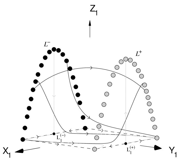
Qualitative Analysis of the Four-Dimensional System

The qualitative dynamics in the full four-dimensional phase space is as follows. In the four-dimensional phase space, the past attractors are the line $L^{-}$ for $X_{1}<\frac{1}{\sqrt{3}}$ and the line $L_{1}$ for $Y_{1}>0$. The future-attractor sets are the lines $L^{+}$ (for $X_{1}>-\frac{1}{\sqrt{3}}$) and $L_{1}$ (for $Y_{1}<0$). Note that $Y_{1}/\sqrt{V_{1}}$ is monotonically increasing. The existence of such a monotonic function excludes the possibility of periodic or recurrent orbits in the full four–dimensional phase space. Therefore, solutions are generically asymptotic to the past to either the $\dot{\varphi}<0$ dilaton–moduli–vacuum solutions (6.7) for $h_{0}<\frac{1}{3}$ or the generalized $\dot{\varphi}<0$ linear dilaton–vacuum solution (6.13) for $n>0$. Similarly, solutions are generically asymptotic to the future to either the $\dot{\varphi}>0$ dilaton–moduli–vacuum solutions (6.7) for $h_{0}>-\frac{1}{3}$ or the generalized $\dot{\varphi}<0$ linear dilaton–vacuum solution (6.13) for $n<0$.

Since $Y_{1}/\sqrt{V_{1}}$ is monotonically increasing, $Y_{1}\rightarrow+1$ or $V_{1}\rightarrow 0$ asymptotically to the future, corresponding to the global sinks on the line $L^{+}$. Similarly, $Y_{1}\rightarrow-1$ or $V_{1}\rightarrow 0$ asymptotically to the past, corresponding to the global sources on the line $L^{-}$. There are also equilibrium sets for the points $Y_{1}=Y_{0}$ inside the phase space. Again, since $Y_{1}/\sqrt{V_{1}}$ is monotonically increasing, the points $Y_{0}<0$ are global sinks and $Y_{0}>0$ are global sources. All of this is consistent with the above discussion concerning asymptotics.

Due to the existence of the monotonic function and the continuity of orbits in the four-dimensional phase space, solutions cannot start and finish on $L_{1}$. Investigation of this invariant set also indicates which sources and sinks are connected; not all orbits from $L^{-}$ can evolve towards $L^{+}$.

Although both lines $L^{\pm}$ lie in both invariant sets $\rho=0$ and $\tilde{K}=0$, the line $L_{1}$ does not, and so both the axion field and curvature term can be dynamically significant at all times (early, intermediate and late) for the corresponding solutions. On the line $L_{1}$, $X_{1}=0$ corresponds to $\dot{\alpha}=0$, and represents static solutions. Similarly, both curvature and axion field are non-zero (and indeed the variables $\rho$, $\tilde{K}$ and $\Lambda$ are proportional to one another). The fact that $\dot{\alpha}=0$ in this case means that neither $\tilde{K}$ nor $\rho$ need be zero, consistent with the analysis of equation (6.15).

6.4.3 The Case $\Lambda>0$, $\tilde{K}<0$

In this case, the negative sign in (6.16) for $U_{2}$ has been chosen as has been the positive sign for $V_{2}$, and the definition $\xi^{2}=\dot{\varphi}^{2}$ is used. The generalized Friedmann constraint equation is now written to read

$$0\leq X_{2}^{2}+Z_{2}+U_{2}+V_{2}\leq 1.$$ (6.27)

For this system $Y_{2}^{2}=1$ and so the four-dimensional system consists of the variables $0\leq\{X_{2}^{2},Z_{2},U_{2},V_{2}\}\leq 1$:

$$\frac{dX_{2}}{dT} = \sqrt{3}\left(1-X_{2}^{2}-Z_{2}-V_{2}-\frac{2}{3}U_{2}\right)+X_{2}\left(1-X_{2}^{2}-Z_{2}\right),$$ (6.28a)

$$\frac{dZ_{2}}{dT} = 2Z_{2}\left(1-X_{2}^{2}-Z_{2}\right)>0,$$ (6.28b)

$$\frac{dU_{2}}{dT} = -2U_{2}\left(X_{2}^{2}+Z_{2}+\frac{1}{\sqrt{3}}X_{2}\right),$$ (6.28c)

$$\frac{dV_{2}}{dT} = -2V_{2}\left(X_{2}^{2}+Z_{2}\right)<0.$$ (6.28d)

The invariant sets $X_{2}^{2}+Z_{2}+U_{2}+V_{2}=1$, $Z_{2}=0$, $V_{2}=0$, $U_{2}=0$ define the boundary of the phase space. The equilibrium sets and their corresponding eigenvalues (denoted by $\lambda$) are

$$S^{+}: X_{2}=-\frac{1}{\sqrt{3}},Z_{2}=0,U_{2}=\frac{2}{3},V_{2}=0;$$ (6.29a)

$$\left(\lambda_{1},\lambda_{2},\lambda_{3},\lambda_{4}\right)=\left(-\frac{2}{3},\frac{2}{3},\frac{4}{3},\frac{4}{3}\right),$$

$$C^{+}: X_{2}=0,Z_{2}=0,U_{2}=0,V_{2}=1;$$ (6.29b)

$$\left(\lambda_{1},\lambda_{2},\lambda_{3},\lambda_{4}\right)=\left(1,0,2,0\right),$$

$$L^{+}: Z_{2}=1-X_{2}^{2},U_{2}=0,V_{2}=0;$$ (6.29c)

$$\left(\lambda_{1},\lambda_{2},\lambda_{3},\lambda_{4}\right)=\left(-\frac{2}{\sqrt{3}}\left[X_{2}+\sqrt{3}\right],-2,0,-2\sqrt{3}\left[X_{2}+\frac{1}{\sqrt{3}}\right]\right).$$

The point $C^{+}$ represents the static ‘linear dilaton–vacuum’ solution (6.12). The saddle $S^{+}$ represents the Milne solution (6.9), where only the curvature term and scale factor are dynamic.

The Invariant Set $\rho=0$ for $\Lambda>0$, $\tilde{K}<0$

In the $\rho=0$ case, the system reduces to three dimensions of $\{X_{2},Z_{2},U_{2}\}$ ($V_{2}=1-X_{2}^{2}-Z_{2}-U_{2}$). The equilibrium sets are the same as above with eigenvalues $\lambda_{1}$, $\lambda_{2}$ and $\lambda_{3}$. Note that for the invariant set $\rho=0$ the entire line $L^{+}$ acts as a global sink, and $C^{+}$ acts as a source (although one of the eigenvalues is zero, this point will be shown to be a source in the full four–dimensional in the next subsubsection and the arguments there equally apply here). Figure 6.4 depicts this three-dimensional phase space.

The variable $Z_{2}$ is monotonically increasing, and as such it is apparent that the modulus field is negligible at early times, but becomes dynamically significant at late times. The existence of such a monotonic function excludes the possibility of periodic or recurrent orbits in this three–dimensional phase space. Generically, solutions asymptote into the past towards the static linear dilaton–vacuum solution (6.12), represented by the point $C^{+}$. Into the future, solutions generically asymptote towards the $\dot{\varphi}>0$ dilaton–moduli–vacuum solution (6.7), represented by the line $L^{+}$.

Figure 6.4: Phase diagram of the system (6.28a) in the NS-NS ($\Lambda>0$) sector with $\rho=0$ and $\tilde{K}<0$. Note that $L^{+}$ represents a line of equilibrium points. See also caption to figure 6.1 on page 6.1.

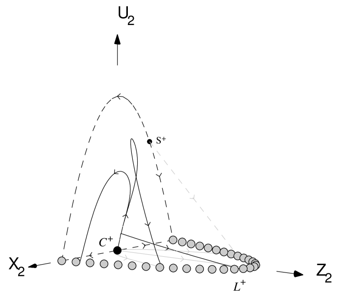
Qualitative Analysis of the Four-Dimensional System

The qualitative behaviour for the invariant set $\tilde{K}=0$ is discussed in subsection 6.4.1 (see figure 6.1 on page 6.1).

In the four-dimensional set, the point $C^{+}$ is non-hyperbolic because of the two zero eigenvalues. However, it can be shown that the point $C^{+}$ is a source in the four-dimensional set by the following argument. Note that the variable $Z_{2}$ is monotonically increasing and hence orbits asymptote into the past towards the invariant set $Z_{2}=0$. Similarly, $V_{2}$ is a monotonically decreasing function, and so orbits asymptote into the past towards large $V_{2}$, which will be shown to be $V_{2}=1$, and therefore towards the point $C^{+}$.

Since $Z_{2}=0$ asymptotically, consider the invariant set $Z_{2}=0$. Equations (6.28a) in this set become

$$\frac{dX_{2}}{dT} = \sqrt{3}\left(1-X_{2}^{2}-V_{2}-\frac{2}{3}\tilde{U}_{2}\right)+X_{2}\left(1-X_{2}^{2}\right),$$ (6.30a)

$$\frac{dU_{2}}{dT} = -2U_{2}\left(X_{2}^{2}+\frac{1}{\sqrt{3}}X_{2}\right),$$ (6.30b)

$$\frac{dV_{2}}{dT} = -2V_{2}X_{2}^{2}.$$ (6.30c)

It is clear from (6.30c) that $V_{2}$ increases monotonically into the past (this is also true for $Z_{2}\neq 0$). Now, this three-dimensional phase space is bounded by the surface $X_{2}^{2}+U_{2}+V_{2}=1$, the “apex” of which lies at $V_{2}=1$ (and $X_{2}=U_{2}=0$). Therefore, all orbits on or inside of the boundary of this phase space lie below $V_{2}=1$, and therefore asymptote into the past towards $V_{2}=1$. To help illustrate that this point is indeed a source, consider the invariant set $Z_{2}=U_{2}=0$, $X_{2}^{2}+V_{2}=1$ in the neighborhood of $C^{+}$. Here equation (6.30a) becomes $dX_{2}/dT=X_{2}(1-X_{2}^{2})$, indicating that orbits are repelled from $X_{2}=0$. Hence, the point $C^{+}$ is the past attractor to the full four-dimensional set. The future attractor for the four-dimensional set is the line $L^{+}$ (for $X_{2}>-\frac{1}{\sqrt{3}}$). Both $C^{+}$ and $L^{+}$ lie in both the invariant sets $\rho=0$ and $\tilde{K}=0$, which is consistent with the analysis of equation (6.15). Generically, solutions are asymptotic in the past to the static, linear dilaton–vacuum solutions (6.12), and to the future to the $\dot{\varphi}>0$ dilaton–moduli–vacuum solutions (6.7), and the curvature terms as well as the axion field are dynamically important only at intermediate times, and are negligible at both early and late times. The variables $Z_{2}$ increases monotonically so that the effect of the modulus field becomes increasingly important dynamically, whilst the variable $V_{2}$ decreases monotonically and so that the effect of the central charge deficit, $\Lambda$, becomes increasing negligible, dynamically. In addition, the existence of monotone functions in the four–dimensional space prohibits closed orbits and serves as proof of the evolution described above.

6.4.4 The Case $\Lambda<0$, $\tilde{K}=0$

In this case, it proves convenient to employ the generalized Friedmann constraint equation (6.6) to eliminate the modulus field rather than the axion field. This equation can be written as

$$1-X_{3}^{2}-\kappa=Z_{3}.$$ (6.31)

The resulting field equations are

$$\frac{dX_{3}}{dT} = \kappa\left(\sqrt{3}+Y_{3}X_{3}\right),$$ (6.32a)

$$\frac{dY_{3}}{dT} = (1-\kappa)\left(1-Y_{3}^{2}\right),$$ (6.32b)

$$\frac{d\kappa}{dT} = -2\kappa\left[\sqrt{3}X_{3}+Y_{3}(1-\kappa)\right].$$ (6.32c)

Note that the invariant set $\dot{\beta}=0$ corresponds to $\kappa=1-X_{3}^{2}$.

The Frozen Modulus ($\dot{\beta}=0$) Invariant Set

Again, the invariant set $\dot{\beta}=0$, corresponding to $\kappa=1-X_{3}^{2}$, is first examined. For this case, the dynamical system becomes equations (6.32a) and (6.32b) with $\kappa=1-X_{3}^{2}$, and the equilibrium points (and their eigenvalues) are given by

$$L^{+}_{(+)}: X_{3}=1,Y_{3}=1;$$ (6.33a)

$$(\lambda_{1},\lambda_{2})=\left(-2,-2[\sqrt{3}+1[\right),$$

$$L^{+}_{(-)}: X_{3}=-1,Y_{3}=1;$$ (6.33b)

$$(\lambda_{1},\lambda_{2})=\left(-2,2[\sqrt{3}X_{3}-1]\right),$$

$$L^{-}_{(+)}: X_{3}=1,Y_{3}=-1;$$ (6.33c)

$$(\lambda_{1},\lambda_{2})=\left(2,-2[\sqrt{3}-1]\right),$$

$$L^{-}_{(-)}: X_{3}=1,Y_{3}=1;$$ (6.33d)

$$(\lambda_{1},\lambda_{2})=\left(2,2[\sqrt{3}+1]\right).$$

Note that $L^{+}_{(-)}$ and $L^{-}_{(+)}$ are saddles, $L^{+}_{(+)}$ is a sink, and $L^{-}_{(-)}$ is a source. The phase portrait is given in figure 6.5.

Figure 6.5: Phase portrait of the system (6.32a) in the NS-NS ($\Lambda<0$) sector for $K=0$ and $\dot{\beta}=0$. See also caption to figure 6.1 on page 6.1.

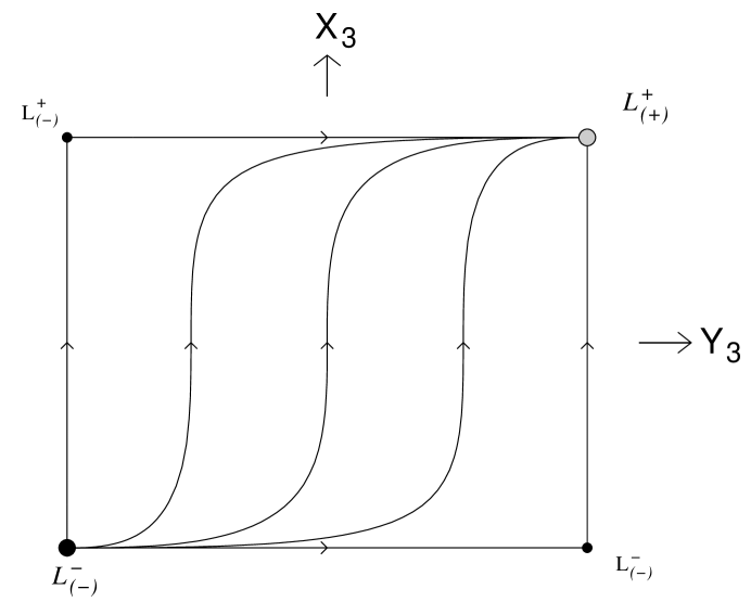
Three–Dimensional System ($\dot{\beta}\neq 0$)

Returning to the three–dimensional system (6.32a), the equilibrium points of this system of ODEs all lie on one of the two lines of non-isolated equilibrium points (or one-dimensional equilibrium sets)

$$L^{\pm}: Y_{3}=\pm 1,\kappa=0;$$ (6.34)

$$(\lambda_{1},\lambda_{2},\lambda_{3})=\left(-2Y_{3},-2(\sqrt{3}X_{3}+Y_{3}),0\right),$$

where $X_{3}$ is arbitrary. These equilibrium sets are normally hyperbolic. The third eigenvalue is zero since this is a set of equilibrium points. Thus, on the line $L^{+}$ the equilibrium points are saddles for $X_{3}<-\frac{1}{\sqrt{3}}$ and local sinks for $X_{3}>-\frac{1}{\sqrt{3}}$. On the line $L^{-}$ the equilibrium points are local sources for $X_{3}<\frac{1}{\sqrt{3}}$ and saddles for $X_{3}>\frac{1}{\sqrt{3}}$. In the two–dimensional invariant set $\dot{\beta}=0$, the points $L^{+}_{(\pm)}$ are the endpoints to the line $L^{+}$ and the points $L^{-}_{(\pm)}$ are the endpoints to the line $L^{-}$. The dynamics is very simple due to the fact that the right-hand sides of equations (6.32a) and (6.32b) are positive–definite and hence $Y_{3}$ and $X_{3}$ are always monotonically increasing functions. The curved upper boundary $\kappa=1-X_{3}^{2}$ denotes the invariant set $\dot{\beta}=0$. The phase diagram is given in figure 6.6.

The lines $L^{\pm}$ represent the “$\mp$” dilaton–moduli–vacuum solutions (6.7); solutions asymptote into the past towards the “$-$” solutions of (6.7) whilst solutions asymptote into the future towards the “$+$” solutions of (6.7).

Figure 6.6: Phase diagram of the system (6.32a) in the NS-NS ($\Lambda<0$) sector for $K=0$ and $\rho\neq 0$. Note that $L^{+}$ and $L^{-}$ represent lines of equilibrium points. The invariant set $\kappa=1-X_{3}^{2}$ portion (upper parabola sheet) is depicted in figure 6.5 on page 6.5. See also caption to figure 6.1 on page 6.1.

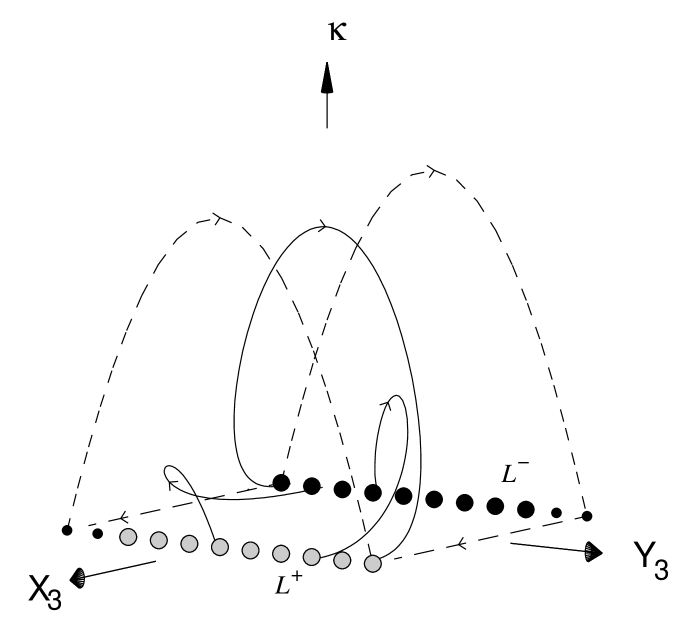
6.4.5 The Case $\Lambda<0$, $\tilde{K}>0$

For this case, $\xi^{2}=\dot{\varphi}^{2}+3\tilde{K}-2\Lambda$ has been chosen and from (6.16) the positive sign for $U_{3}$ is chosen as is the negative sign for $V_{3}$ in order for these variables to be positive definite. The generalized Friedmann constraint equation can be rewritten as

$$0\leq X_{3}^{2}+Z_{3}\leq 1,\qquad Y_{3}^{2}+U_{3}+V_{3}=1,$$ (6.35)

and again $U_{3}$ (which is proportional to $\tilde{K}$) may be eliminated, yielding the four-dimensional system of ODEs for $0\leq\{X_{3}^{2},Y_{3}^{2},Z_{3},V_{3}\}\leq 1$:

$$\frac{dX_{3}}{dT} = \left(1-X_{3}^{2}-Z_{3}\right)\!\!\left(\sqrt{3}\!+\!X_{3}Y_{3}\right)-\!\frac{1}{\sqrt{3}}\left(1\!-\!Y_{3}^{2}\!-\!V_{3}\right)\!\!\left(1\!-\!X_{3}^{2}\!-\!Z_{3}\right),$$ (6.36a)

$$\frac{dY_{3}}{dT} = \frac{1}{\sqrt{3}}X_{3}Y_{3}\left(1-Y_{3}^{2}-V_{3}\right)+\left(1-Y_{3}^{2}\right)\left(X_{3}^{2}+Z_{3}\right),$$ (6.36b)

$$\frac{dZ_{3}}{dT} = 2Z_{3}\left[\frac{1}{\sqrt{3}}X_{3}\left(1-Y_{3}^{2}-V_{3}\right)+Y_{3}\left(1-X_{3}^{2}-Z_{3}\right)\right],$$ (6.36c)

$$\frac{dV_{3}}{dT} = 2V_{3}\left[\frac{1}{\sqrt{3}}X_{3}\left(1-Y_{3}^{2}-V_{3}\right)-Y_{3}\left(X_{3}^{2}+Z_{3}\right)\right].$$ (6.36d)

The invariant sets $Y_{3}^{2}+V_{3}=1$, $X_{3}^{2}+Z_{3}=1$, $Z_{3}=0$ define the boundary of the phase space. The only equilibrium set and its corresponding eigenvalues (denoted by $\lambda$) are

$$L^{\pm}: Y_{3}=\pm 1,Z_{3}=1-X_{3}^{2},V_{3}=0;$$ (6.37a)

$$\left(\lambda_{1},\lambda_{2},\lambda_{3},\lambda_{4}\right)\!=\!\left(\mp\frac{2}{\sqrt{3}}\left[\sqrt{3}\!\pm\!X_{3}\right],\mp 2,0,\mp 2\sqrt{3}\left[\frac{1}{\sqrt{3}}\!\pm\!X_{3}\right]\right),$$

where again the zero eigenvalues arise because these are all lines of equilibrium points. Here, the global sink is the line $L^{+}$ for $X_{3}>-\frac{1}{\sqrt{3}}$, and the global source is the line $L^{-}$ for $X_{3}<\frac{1}{\sqrt{3}}$. The exact solutions corresponding to these two lines are the dilaton–moduli–vacuum solutions given by equation (6.7).

The Invariant Set $\rho=0$ for $\Lambda<0$, $\tilde{K}>0$

Because $\dot{\alpha}\neq 0$ at the equilibrium sets, the $\rho=0$ case is examined, in which the system reduces to three dimensions $\{X_{3},Y_{3},V_{3}\}$ ($Z_{3}=1-X_{3}^{2}$). The equilibrium sets are the same as above with eigenvalues $\lambda_{1}$, $\lambda_{2}$, $\lambda_{3}$. Note that the entire line $L^{+}$ acts as a global sink and that the entire line $L^{-}$ acts as a global source in this three–dimensional invariant set. Figure 6.7 depicts this three-dimensional phase space.

The function $Y_{3}/\sqrt{V_{3}}$ is monotonically increasing, eliminating the possibility of periodic orbits. Therefore, solutions generically asymptote into the past towards the $\dot{\varphi}<0$ dilaton–moduli–vacuum solutions (6.7), and into the future towards the $\dot{\varphi}>0$ dilaton–moduli–vacuum solutions (6.7). The curvature term and central charge deficit are dynamically significant only at intermediate times.

Figure 6.7: Phase diagram of the system (6.36a) in the NS-NS ($\Lambda<0$) sector for $\rho=0$ and $\tilde{K}>0$. Note that $L^{+}$ and $L^{-}$ represent lines of equilibrium points. See also caption to figure 6.1 on page 6.1.

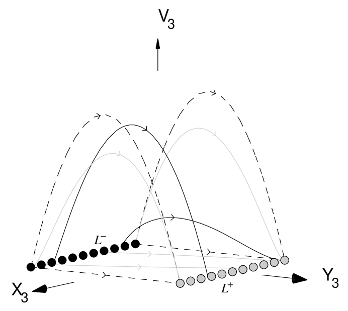
Qualitative Analysis of the Four-Dimensional System

The qualitative dynamics in the full four-dimensional phase space is as follows. The global repellors and attractors of this phase space are the lines $L^{-}$ and $L^{+}$, respectively, corresponding to the dilaton–moduli–vacuum solutions. Hence orbits generically asymptote into the past towards the line $L^{-}$ (for $X_{3}<\frac{1}{\sqrt{3}}$), and generically asymptote into the future towards the line $L^{+}$ (for $X_{3}>-\frac{1}{\sqrt{3}}$); both lines lie in both of the invariant sets $\rho=0$ and $\tilde{K}=0$, consistent with the analysis of equation (6.15). Hence, solutions generically asymptote into the past towards the $\dot{\varphi}<0$ dilaton–moduli–vacuum solutions (6.7) for $h_{0}<\frac{1}{3}$, and into the future towards the $\dot{\varphi}>0$ dilaton–moduli–vacuum solutions (6.7) for $h_{0}>-\frac{1}{3}$. Again, the curvature term, the axion field and the central charge deficit are dynamically important only at intermediate times, and are negligible at early and late times. The existence of the monotonically increasing function $Y_{3}/\sqrt{V_{3}}$ excludes the possibility of periodic orbits and serves to verify that the evolution of solutions in the four–dimensional set discussed above.

6.4.6 The Case $\Lambda<0$, $\tilde{K}<0$

The negative signs are chosen for both $U_{4}$ and $V_{4}$ from (6.16) in this case, and the definition $\xi^{2}=\dot{\varphi}^{2}-2\Lambda$ is chosen. The generalized Friedmann constraint equation is now written to read

$$0\leq X_{4}^{2}+Z_{4}+U_{4}\leq 1,\qquad Y_{4}^{2}+V_{4}=1,$$ (6.38)

where now $V_{4}$ is considered to be the extraneous variable, resulting is the four-dimensional system consisting of the variables $0\leq\{X_{4}^{2},Y_{4}^{2},Z_{4},U_{4}\}\leq 1$:

$$\frac{dX_{4}}{dT} = \left(1-X_{4}^{2}-Z_{4}\right)\left(\sqrt{3}+X_{4}Y_{4}\right)-\frac{2}{\sqrt{3}}U_{4},$$ (6.39a)

$$\frac{dY_{4}}{dT} = \left(1-Y_{4}^{2}\right)\left(X_{4}^{2}+Z_{4}\right)>0,$$ (6.39b)

$$\frac{dZ_{4}}{dT} = 2Z_{4}Y_{4}\left(1-X_{4}^{2}-Z_{4}\right),$$ (6.39c)

$$\frac{dU_{4}}{dT} = -2U_{4}\left[Y_{4}\left(X_{4}^{2}+Z_{4}\right)+\frac{1}{\sqrt{3}}X_{4}\right].$$ (6.39d)

The invariant sets $X_{4}^{2}+Z_{4}+U_{4}=1$, $Z_{4}=0$, $Y_{4}^{2}=1$, $U_{4}=0$ define the boundary of the phase space. The equilibrium sets and their corresponding eigenvalues (denoted by $\lambda$) are

$$S^{\pm}: X_{4}=\mp\frac{1}{\sqrt{3}},Y_{4}=\pm 1,Z_{4}=0,U_{4}=\frac{2}{3};$$ (6.40a)

$$\left(\lambda_{1},\lambda_{2},\lambda_{3},\lambda_{4}\right)=\left(\pm\frac{2}{3},\mp\frac{2}{3},\pm\frac{4}{3},\pm\frac{4}{3}\right),$$

$$L^{\pm}: Y_{4}=\pm 1,Z_{4}=1-X_{4}^{2},U_{4}=0;$$ (6.40b)

$$\left(\lambda_{1},\lambda_{2},\lambda_{3},\lambda_{4}\right)=\left(\mp\frac{2}{\sqrt{3}}\left[\sqrt{3}\!\pm\!X_{4}\right],\mp 2,0,\mp 2\sqrt{3}\left[\frac{1}{\sqrt{3}}\!\pm\!X_{4}\right]\right)\!.$$

The global source for this system is the line $L^{-}$ (for $X_{4}<\frac{1}{\sqrt{3}}$), and the global sink is the line $L^{+}$ (for $X_{4}>-\frac{1}{\sqrt{3}}$). These lines correspond to the dilaton–moduli–vacuum solutions, given by equation (6.7). The saddle points $S^{\pm}$ represent the Milne models (6.9).

The Invariant Set $\rho=0$ for $\Lambda<0$, $\tilde{K}<0$

In the $\rho=0$ case, the system reduces to three dimensions of $\{X_{4},Y_{4},Z_{4}\}$ ($U_{4}=1-X_{4}^{2}-Z_{4}$). The equilibrium sets are the same as above with eigenvalues $\lambda_{1}$, $\lambda_{2}$, $\lambda_{3}$. Note that for the invariant set $\rho=0$ the entire line $L^{+}$ acts as a global sink and the entire line $L^{-}$ acts as a global source. The variable $Y_{4}$ is monotonically increasing, the existence of which excludes the possibility or recurrent orbits. Hence, solutions generically asymptote into the past towards the $\dot{\varphi}<0$ dilaton–moduli–vacuum solutions (6.7), and into the future towards the $\dot{\varphi}>0$ dilaton–moduli–vacuum solutions (6.7). The curvature and central charge deficit are dynamically significant only at intermediate times. Figure 6.8 depicts this three-dimensional phase space.

Figure 6.8: Phase diagram of the system (6.39a) in the NS-NS ($\Lambda<0$) sector with $\rho=0$ and $\tilde{K}<0$. Note that $L^{+}$ and $L^{-}$ represent lines of equilibrium points. See also caption to figure 6.1 on page 6.1.

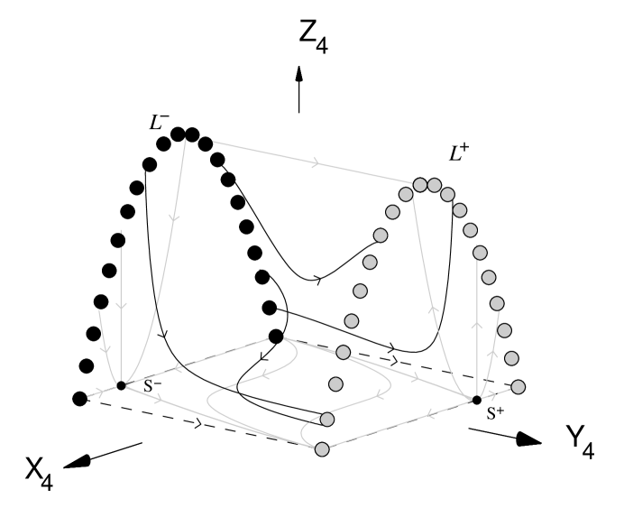
Qualitative Analysis of the Four-Dimensional System

The dynamical behaviour in the invariant set $\tilde{K}=0$ is identical to that described in subsection 6.4.6 (see figure 6.4.4).

The qualitative dynamics in the full four-dimensional phase space is as follows. Note that $Y_{4}$ is monotonically increasing and so orbits asymptote into the past towards $Y_{4}=-1$ and into the future towards $Y_{4}=+1$. Again, the existence of such monotonic functions exclude the possibility of periodic orbits in the four–dimensional phase space. Most orbits asymptote into the past towards the line $L^{-}$ (for $X_{4}<\frac{1}{\sqrt{3}}$), and into the future towards the line $L^{+}$ (for $X_{4}>-\frac{1}{\sqrt{3}}$). Both lines $L^{\pm}$ lie in both invariant sets $\rho=0$ and $\tilde{K}=0$, which is consistent with the analysis of equation (6.15). Generically, solutions asymptote to the past to the $\dot{\varphi}<0$ dilaton–moduli–vacuum solutions (6.7) for $h_{0}<\frac{1}{3}$, and to the future to the $\dot{\varphi}>0$ dilaton–moduli–vacuum solutions (6.7) for $h_{0}>-\frac{1}{3}$. The variable $Y_{4}$ increases monotonically along orbits and so $\dot{\varphi}$ is dynamically significant at early and late times, but dynamically negligible at intermediate times. Conversely, it can be seen that the curvature, the central charge deficit and the axion field are dynamically important only at intermediate times, and are negligible at both early and late times.

6.5 Summary of Analysis in the Jordan Frame

This discussion begins with two tables; Table 6.1 lists which terms are the dominant variables for each equilibrium set as well as the deceleration parameter, $q$, for the corresponding model and Table 6.2 lists the attracting behaviour of the equilibrium sets.

Set	Dominant Variables								$q$	H
$L^{+}$ ($t<0$)	$\alpha$	$\hat{\Phi}$	$\dot{\beta}$						$-(1+h_{0})h_{0}^{-1}$	$h_{0}(-t)^{-1}$
$L^{-}$ ($t>0$)	$\alpha$	$\hat{\Phi}$	$\dot{\beta}$						$(1-h_{0})h_{0}^{-1}$	$h_{0}t^{-1}$
$C^{\pm}$		$\hat{\Phi}$				$\Lambda>0$			$0$	$0$
$L_{1}$		$\hat{\Phi}$		$\dot{\sigma}$	$k\geq 0$	$\Lambda>0$			$0$	$0$
$S^{\pm}$	$\alpha$				$k<0$				$0$	$t^{-1}$

Table 6.1: The dominant variables for each equilibrium set as well as the equilibrium set’s deceleration parameter, $q$, and Hubble parameter $H$. Inflation occurs when $q<0$ and $H>0$, whereas “deflation” occurs for $q>0$ and $H<0$. Note that the only “anisotropic” solutions are represented by the lines $L^{\pm}$, except when $h_{0}^{2}=\frac{1}{3}$.

Note that the only inflationary models are those represented by $L^{+}$ (for $h_{0}>0$).

Terms Present					Early	Intermediate	Late
$\dot{\beta}$		$\Lambda>0$			$C^{+}$	$L^{+}$	$L^{+}$
$\dot{\beta}$	$k>0$	$\Lambda>0$			$L_{1}$, $L^{-}$	$L^{\pm}$	$L_{1}$, $L^{+}$
$\dot{\beta}$	$k<0$	$\Lambda>0$			$C^{+}$	$S^{+}$, $L^{+}$	$L^{+}$
$\dot{\beta}$	$k\geq 0$	$\Lambda<0$			$L^{-}$	$L^{\pm}$	$L^{+}$
$\dot{\beta}$	$k<0$	$\Lambda<0$			$L^{-}$	$S^{\pm}$, $L^{\pm}$	$L^{+}$

Table 6.2: Summary of the early-time, intermediate, and late-time attractors for the various models examined. Note that $\dot{\alpha}$, $\hat{\Phi}$ and $\dot{\sigma}$ are present in every model.

For every case studied, monotonic functions have been established which precludes the existence of recurrent or periodic orbits, thereby allowing the early-time and late-time behaviour conclusions to be made based upon the equilibrium sets of the system. In all cases, the dilaton–moduli–vacuum solutions act as either early-time or late-time attractors (and, in many of the cases, both). Because these solutions lie in both the $\rho=0$ and $\tilde{K}=0$ invariant sets and contain no central charge deficit, it is conclusive that the modulus and dilaton fields are dynamically important asymptotically. Furthermore, with the exception of the $\Lambda>0$, $\tilde{K}>0$ case, all early-time and late-time attracting sets lie in either the $\rho=0$ invariant set, or the $\tilde{K}=0$ invariant set, and a majority of these sets lie in both; thus, there seems to be a generic feature in which the curvature and the axion field are dynamically significant at intermediate times and are asymptotically negligible at early and at late times. The exception to this generic behaviour is the $\Lambda>0$, $\tilde{K}>0$ case, where the generalized linear dilaton–vacuum solution (6.13), in which neither $\rho=0$ nor $\tilde{K}=0$, acts both as a repellor (for $\dot{\varphi}>0$) and as an attractor (for $\dot{\varphi}<0$). In these solutions, the variables $\rho$ and $\tilde{K}$ are proportional to the central charge deficit, $\Lambda$.

When $\Lambda<0$, the central charge deficit is dynamically significant only at intermediate times. The only repelling and attracting sets in this instance are the dilaton–moduli–vacuum solutions. When $\tilde{K}>0$, the central charge deficit can be dynamically significant at early and at late times, and the corresponding solutions are the generalized dilaton–vacuum solutions (6.13), represented by the line $L_{1}$. When $\tilde{K}>0$, these solutions can be repelling ($\dot{\varphi}>0$) and attracting ($\dot{\varphi}<0$). When $\tilde{K}<0$, then the endpoint of this line, $C^{+}$ (representing equation (6.12)) is a repellor.

Typically, the curvature term is found to be be dynamically significant only at intermediate times, and is asymptotically negligible. However, the only exceptions to this is the case $\Lambda>0$, $\tilde{K}>0$ where the generalized linear dilaton–vacuum attractors and repellors have a non-negligible curvature.

The field equations derived from action (1.28) for this background for $\Lambda_{\rm M}=Q=0$ are formally identical to those for either FRW models with a modulus field or certain Bianchi models with or without a modulus field. With an anisotropic model, however, the variables $\alpha$ and $\beta$ now parameterize the averaged scale factor and the shear parameter of the universe, respectively. More generally, a finite number of modulus fields and shear modes can be introduced by defining the variable $6\dot{\beta}^{2}$ via equation (6.4). If isotropization is defined by $\dot{\beta}\rightarrow 0$, then the only anisotropic models are the dilaton–moduli-vacuum solutions (6.7). These solutions are attracting solutions (either into the past or future) for most models. However, these are not the only asymptotic solutions and all other solutions mentioned in this chapter are isotropic ($\dot{\beta}=0$). In particular, the models in which $\Lambda>0$ and $k>0$ do have isotropic late-time attractors.

The only attracting solutions which are inflationary are the dilaton–moduli–vacuum solutions (the “$-$” branch of (6.7) for $h_{0}>0$) which occur in the pre-big bang portion of the theory. Note that the time reverse dynamics of these models correspond to $\dot{\alpha}\rightarrow-\dot{\alpha}$ (i.e., contracting $\rightarrow$ expanding and vice versa) as well as $\dot{\varphi}\rightarrow-\dot{\varphi}$ and correspond to a post-big bang era. Hence, all late–time attracting solutions in the post-big bang regime are not inflationary.

6.6 Exact Solutions in the Einstein Frame

The analysis of this chapter can equally be applied in the Einstein frame, resulting in the same equilibrium points. This section describes the solutions of the equilibrium point in the Einstein frame and then relates the quantities $\{\dot{\beta},\dot{\sigma}\,\Lambda,\Lambda_{\rm M},Q\}$ in terms of matter fields, as described in Chapter 2, thereby mathematically casting the analysis into a theory of general relativity containing a matter source and a scalar field with exponential potential.

First, the transformation (2.10) on page 2.10 between the scalar fields $\phi$ and $\Phi$ for $\omega_{0}=-1$ is rewritten as

$$\frac{dt^{*}}{dt}=\pm e^{\pm\phi/\sqrt{2}}\equiv e^{-\varepsilon\phi/\sqrt{2}};$$ (6.41)

i.e., the “$\pm$” sign before the exponential term is explicitly taken to be “$+$” to ensure that $t^{*}$ (time in the Einstein frame) and $t$ (time in the Jordan frame) grow in the same direction which ensures that $\!\,{}^{{}^{\mbox{\rm\tiny(sf)}}}\!H$ and $\!\,{}^{{}^{\mbox{\rm\tiny(st)}}}\!H$ are of the same sign when $\phi=\phi_{0}$ ($\Phi=\Phi_{0}$), and the “$\pm$” sign inside the exponential term is replaced with the constant $\varepsilon=\mp 1$ to save confusion with the “$\pm$” signs to follow in the exact solutions.

To refresh, the scale factors between the two frames are related by

$$a^{*}=e^{-\frac{1}{2}\hat{\Phi}}a\qquad\Leftrightarrow\qquad a=e^{\varepsilon\phi/\sqrt{2}}a^{*},$$ (6.42)

where $a^{*}$ is the scale factor in the Einstein frame and $a$ is the scale factor in the Jordan frame.

The dilaton–moduli–vacuum solutions transform to the Einstein frame as

$$L^{\mp}: a^{*}=a^{*}_{0}\left|t_{*}\right|^{\frac{1}{3}}\qquad\Rightarrow\qquad\!\,^{{}^{\mbox{\rm\tiny(sf)}}}\!H=\frac{1}{3}t_{*}^{-1}\qquad\Rightarrow\qquad\!\,^{{}^{\mbox{\rm\tiny(sf)}}}\!q=2,$$ (6.43)

$$e^{\phi}=e^{\bar{\phi}^{*}_{0}}\left|t_{*}\right|^{\frac{\varepsilon\sqrt{2}(\pm 3h_{0}-1)}{3(1\mp h_{0})}},$$

$$e^{\beta}=e^{\beta^{*}_{0}}\left|t_{*}\right|^{\frac{\pm\sqrt{2(1-3h_{0}^{2})}}{3\sqrt{3}(1\mp h_{0})}},$$

$$\sigma=\sigma_{0},$$

$$k=0,$$

where $\{a^{*}_{0},\bar{\phi}^{*}_{0},\beta^{*}_{0}\}$ are suitable redefined integration constants to absorb positive definite constants which arise from (6.41) and (6.42), and again the $\pm$ sign corresponds to the sign of $t_{*}$. Note that in the Einstein frame, the scale factor does not depend on the constant $h_{0}$. From $\!\,{}^{{}^{\mbox{\rm\tiny(sf)}}}\!H$ and $\!\,{}^{{}^{\mbox{\rm\tiny(sf)}}}\!q$, it is apparent that $L^{+}$ represents deflationary models, whereas $L^{-}$ represents expanding, non-inflationary models. This is substantially different than from the Jordan frame, where inflationary models exist for $t_{*}<0$. From the analysis of the previous sections, $L^{-}$ is an early-time attractor for most models considered and $L^{+}$ is a late-time attractor for most models. In all models considered $L^{\pm}$ are also saddle points.

In the Einstein frame, the saddle-point Milne solution becomes

$$S^{\mp}: a^{*}=a^{*}_{0}\left(\pm t_{*}\right)\qquad\Rightarrow\qquad\!\,^{{}^{\mbox{\rm\tiny(sf)}}}\!H=t_{*}^{-1}\qquad\Rightarrow\qquad\!\,^{{}^{\mbox{\rm\tiny(sf)}}}\!q=0,$$ (6.44)

$$\phi=\phi_{0},$$

$$\beta=\beta_{0},$$

$$\sigma=\sigma_{0},$$

$$k=-a_{0}^{2},$$

where $a^{*}_{0}=a_{0}$. Again, the “$\pm$” sign corresponds to the sign of $t_{*}$. These solutions are a saddle solutions in all models where $\Lambda\neq 0$ and $k\neq 0$.

The static linear dilaton–vacuum solution in the Einstein frame becomes

$$C^{\mp}: a^{*}=a^{*}_{0}\left|t_{*}\right|\qquad\Rightarrow\qquad\!\,^{{}^{\mbox{\rm\tiny(sf)}}}\!H=t_{*}^{-1}\qquad\Rightarrow\qquad\!\,^{{}^{\mbox{\rm\tiny(sf)}}}\!q=0,$$ (6.45)

$$e^{\varepsilon\sqrt{2}\phi}=\frac{2}{\Lambda t_{*}^{2}},$$

$$\beta=\beta_{0},$$

$$\sigma=\sigma_{0},$$

$$k=0,$$

where $a^{*}_{0}=\sqrt{\frac{1}{2}\Lambda}a_{0}$. The solution $C^{+}$ is an early-time attractor for all $\Lambda>0$ models considered (except when $k>0$ in which case this solution is replaced by its generalization $L_{1}$ discussed below), and $C^{-}$ arises as a late-time attractor in the model where $\Lambda>0$ and $\Lambda_{\rm M}<0$ (chapter 8). Unlike in the Jordan frame in which the universe is static, in the Einstein frame the universe is linearly contracting for $t_{*}<0$ and linearly expanding for $t_{*}>0$.

The generalized linear dilaton–vacuum solutions in the Einstein frame become

$$L_{1}: a=a^{*}_{0}\left|t_{*}\right|\qquad\Rightarrow\qquad\!\,^{{}^{\mbox{\rm\tiny(sf)}}}\!H=t_{*}^{-1}\qquad\Rightarrow\qquad\!\,^{{}^{\mbox{\rm\tiny(sf)}}}\!q=0,$$ (6.46)

$$e^{\varepsilon\sqrt{2}\phi}=\frac{2\left(2+n^{2}\right)}{3n^{2}\Lambda t_{*}^{2}},$$

$$\beta=\beta_{0},$$

$$\sigma=\sigma_{0}\pm\frac{\sqrt{6n^{2}\left(1-n^{2}\right)}}{2\left(2+n^{2}\right)}\Lambda t_{*}^{2},$$

$$k=\frac{2(1-n^{2})}{3n^{2}}a^{*2}_{0},$$

where $n\in[-1,1]$. Here the $n<0$ solutions correspond to $t_{*}>0$, representing positively-curved, expanding models whereas $n>0$ (corresponding to $t_{*}<0$) represent contracting models. Again, this is a different behaviour than that in the Jordan frame wherein the models are static. As determined in the analysis in sections 6.4.2, for $\Lambda>0$ and $k>0$, $L_{1}$ represents early-time attracting solutions for $n>0$ and late-time attracting solutions for $n<0$.

In the Einstein frame, there are no inflationary late-time attracting solutions.

6.6.1 Mathematical Equivalence to Matter Terms in the Einstein Frame

As mentioned in Chapter 2, these string models are mathematically equivalent (in the Einstein frame) to a theory of general relativity containing a matter source and a scalar field with an exponential potential; i.e., $V=V_{0}e^{k\phi}$, where either $k^{2}=2$ or $V_{0}=0$. This subsection is devoted to explicitly determining the form of the matter field for each of the equilibrium sets discussed in this chapter. Before each case is examined, it is useful to restate that upon transformation from the Jordan frame into the Einstein frame, interaction terms arise so that each source (matter field and scalar field) will not be separately conserved. In fact, the conservation equations in the Einstein frame can be typically written as

$$\dot{\phi}\left(\ddot{\phi}+3\!\,^{{}^{\mbox{\rm\tiny(sf)}}}\!H\dot{\phi}+\frac{dV}{d\phi}\right) = -\delta,$$ (6.47a)

$$\dot{\mu}+3\!\,^{{}^{\mbox{\rm\tiny(sf)}}}\!H\left(\mu+p\right) = +\delta.$$ (6.47b)

Furthermore, in each instance, the total energy density and pressure of the scalar field may be calculated, namely,

$$\mu_{\phi} = \frac{1}{2}\dot{\phi}^{2}+V,$$ (6.48a)

$$p_{\phi} = \frac{1}{2}\dot{\phi}^{2}-V,$$ (6.48b)

and hence $\gamma_{\phi}\equiv(\mu_{\phi}+p_{\phi})/\mu_{\phi}$ can be compared with the $\gamma$ of the matter field.

For these models there are two scenarios from which to choose:

1. $V=\Lambda e^{\sqrt{2}\varepsilon\phi}$ $(k^{2}=2)$, ${\cal U}=0$
   The interaction term for this case is $\delta=-2\sqrt{2}\varepsilon\dot{\phi}\ p$.

2. $V=0$, ${\cal U}=\Lambda e^{\sqrt{2}\varepsilon\phi}$
   The interaction term for this case is $\delta=-\frac{\sqrt{2}}{2}\varepsilon\dot{\phi}(\mu+3p)$.

For these two scenarios, the matter field is defined by

$$\mu \equiv \frac{1}{4}\dot{\sigma}^{2}e^{2\sqrt{2}\varepsilon\phi}+{\cal U}$$ (6.49a)

$$p \equiv \frac{1}{4}\dot{\sigma}^{2}e^{2\sqrt{2}\varepsilon\phi}-{\cal U}$$ (6.49b)

and do not in general represent barotropic matter with a linear equation of state [$p=(\gamma-1)\mu$], although the equations of state are linear at the equilibrium points. Tables 6.3 and 6.4 list $\{\mu,p,\gamma,\mu_{\phi},p_{\phi},\gamma_{\phi},\delta\}$ for each equilibrium set in each of the two scenarios discussed above.

Scenario A:   $V=\Lambda e^{\sqrt{2}\varepsilon\phi}$,   ${\cal U}=0$,   $\delta=-2\sqrt{2}\varepsilon\dot{\phi}\ p$
Set	$\mu$	$p$	$\gamma$	$\mu_{\phi}$	$p_{\phi}$	$\gamma_{\phi}$	$\delta$
$L^{\pm}$	$0$	$0$	$-$	$\frac{(\pm 3h_{0}-1)^{2}}{9(1\mp h_{0})^{2}}t_{*}^{-2}$	$\mu_{\phi}$	$2$	$0$
$S^{\pm}$	$0$	$0$	$-$	$0$	$0$	$-$	$0$
$C^{\pm}$	$0$	$0$	$-$	$3t_{*}^{-2}$	$-t_{*}^{-2}$	$\frac{2}{3}$	$0$
$L_{1}$	$\frac{2(1-n^{2})}{3n^{2}}t_{*}^{-2}$	$\mu$	$2$	$\frac{4+5n^{2}}{3n^{2}}t_{*}^{-2}$	$\frac{n^{2}-4}{3n^{2}}t_{*}^{-2}$	$\frac{6n^{2}}{4+5n^{2}}\in[0,\frac{2}{3}]$	$\frac{8(1-n^{2})}{3n^{2}}t_{*}^{-3}$

Table 6.3: The matter terms ($\mu$, $p$, $\gamma$) as well as $\mu_{\phi}$, $p_{\phi}$, $\gamma_{\phi}$ and $\delta$ for each of the equilibrium sets derived in scenario A for $\Lambda_{\rm M}=Q=0$.

From section 6.5, the asymptotic behaviour of the models in the Einstein frame is known and comments on which solutions represent asymptotic states in the Einstein frame are equally applicable here.

In scenario A, it is evident that asymptotically the matter field either vanish (represented by the sets $L^{\pm}$ or $C^{\pm}$) or asymptote towards a stiff equation of state (represented by the set $L_{1}$), the latter arising only in the case of negative curvature. There are no matter scaling solutions at the equilibrium sets except the trivial case of the saddle Milne model, in which all sources are zero.

Scenario B:   $V=0$,  ${\cal U}=\Lambda e^{\sqrt{2}\varepsilon\phi}$,   $\delta=-\frac{\sqrt{2}}{2}\varepsilon\dot{\phi}(\mu+3p)$
Set	$\mu$	$p$	$\gamma$	$\mu_{\phi}$	$p_{\phi}$	$\gamma_{\phi}$	$\delta$
$L^{\pm}$	$0$	$0$	$-$	$\frac{(\pm 3h_{0}-1)^{2}}{9(1\mp h_{0})^{2}}t_{*}^{-2}$	$\mu_{\phi}$	$2$	$0$
$S^{\pm}$	$0$	$0$	$-$	$0$	$0$	$-$	$0$
$C^{\pm}$	$2t_{*}^{-2}$	$-\mu$	$0$	$t_{*}^{-2}$	$\mu_{\phi}$	$2$	$-4t_{*}^{-3}$
$L_{1}$	$\frac{2}{n^{2}}t_{*}^{-2}$	$\frac{-2(1+2n^{2})}{3n^{2}}t_{*}^{-2}$	$\frac{2}{3}(1-n^{2})\in[0,\frac{2}{3}]$	$t_{*}^{-2}$	$\mu_{\phi}$	$2$	$-4t_{*}^{-3}$

Table 6.4: The matter terms ($\mu$, $p$, $\gamma$) as well as $\mu_{\phi}$, $p_{\phi}$, $\gamma_{\phi}$ and $\delta$ for each of the equilibrium sets derived in scenario B for $\Lambda_{\rm M}=Q=0$.

In scenario B, it is evident that asymptotically the matter field vanishes as trajectories asymptote to $L^{\pm}$ or $C^{\pm}$ (which is the same behaviour for scenario A). However, for trajectories asymptoting towards the line $L_{1}$ (for negatively curved models), the matter field asymptotes to a linear equation of state with $0\leq\gamma<\frac{2}{3}$. Again, there are no matter scaling solutions at any of the equilibrium sets.

Chapter 7 String Models II: Non-Zero Cosmological Constant ($\Lambda=Q=0$)

In this chapter, $\Lambda=0$ and $Q=0$ in order to determine the rôle of $\Lambda_{\rm M}$ in the dynamics of the system (6.5a). As demonstrated in the last chapter, most of the analysis to follow is equally applicable to curved FRW models with a modulus field and to certain Bianchi type I, V and IX models with or without a modulus field. The chapter is organized as follows. In section 7.2, the field equations (6.5a) and (6.6) are reexamined with $\Lambda=0$ and $Q=0$, and all the known corresponding exact solutions are listed in section 7.1 for $\Lambda_{\rm M}\neq 0$. It was shown in section 6.3 that for most cases either the curvature or the axion field will asymptotically dominate at early or late times, and hence the four-dimensional dynamical system can be reduced to a three-dimensional system. There was one exception to this comment which existed only in the NS-NS case and hence the analysis there is completely applicable to this chapter. Section 7.3 proceeds with the analysis of the equations. The chapter ends with a summary section and a section which discusses the corresponding solutions and asymptotic behaviour in the Einstein frame. Again, this chapter is primarily confined to the Jordan frame (except the final section), and so the index “(st)” shall be omitted to save notation, (but must be introduced again in the final section when both frames are discussed).

7.1 Exact Solutions in the Matter Sector

There are several exact solutions which exist for $\Lambda_{\rm M}\neq 0$ and $\Lambda=Q=0$ which are represented by equilibrium points found in the analysis of this chapter.

The solution found in Billyard et al. [105] is given by

$$a = a_{0}\left[\frac{\sqrt{3\Lambda_{\rm M}}}{4}\left|t\right|\right]^{\frac{1}{3}},$$

$$\hat{\Phi} = -\ln\left[\frac{3\Lambda_{\rm M}}{16}t^{2}\right],$$

$$\beta = \beta_{0},$$

$$\sigma = \sigma_{0}\pm\frac{\sqrt{15}}{16}\Lambda_{\rm M}t^{2},$$

$$k = 0,$$ (7.1)

where $\{a_{0},\beta_{0},\sigma_{0}\}$ are arbitrary constants and time is defined over the interval $t<0$ ($\dot{\varphi}>0$) for the equilibrium point $S^{+}_{1}$ and $t>0$ $(\dot{\varphi}<0$) for the equilibrium point $S^{-}_{1}$. Note that $S^{+}_{1}$ represents a deflationary model (i.e. $q>0$ and $H<0$).

The negative-curvature cosmological model is given by

$$a = \frac{1}{2}a_{0}\sqrt{\Lambda}_{\rm M}\left|t\right|,$$

$$\hat{\Phi} = -\ln\left[\frac{1}{4}\Lambda_{\rm M}t^{2}\right],$$

$$\beta = \beta_{0},$$

$$\sigma = \sigma_{0},$$

$$k = -\frac{3}{4}\Lambda_{\rm M}a_{0}^{2}$$

where $\{a_{0},\beta_{0},\sigma_{0}\}$ are integration constants and the time is defined for $t<0$. This solution is represented by the equilibrium point $N$ throughout this chapter.

For the $\tilde{K}=0$, $\Lambda_{\rm M}>0$ case (section 7.3.1), there exists an invariant line which connects the point “$S_{1}^{+}$” (i.e. equation (7.1)) to the line $L^{+}$ for $\mu_{1}=-\frac{1}{\sqrt{27}}$ (i.e. the “$-$” solution of equation (6.7) for $h_{0}=-\frac{1}{9}$). In terms of cosmic time, $t$, this exact solution satisfies

$$\Lambda_{\rm M}e^{\varphi+3\alpha}-\frac{16}{27}\dot{\varphi}^{2}+\frac{288}{13}\dot{\beta}^{2}=0,$$ (7.3)

and

$$\dot{\alpha}=-\frac{1}{9}\dot{\varphi},$$ (7.4)

whence equations (6.5a) and (6.6) yield

$$\ddot{\varphi}=\dot{\varphi}^{2}+k_{\varphi}^{2}e^{2\varphi},$$ (7.5)

which is a second-order ODE for $\varphi$, where $k_{\varphi}$ is an integration constant. Defining

$$\varrho\equiv\frac{e^{-\varphi}}{k_{\varphi}},$$ (7.6)

this equation simplifies to

$$\varrho\ddot{\varrho}=-1,$$ (7.7)

which can be integrated exactly to obtain $\dot{\varphi}$ [187] and a second integration then yields $\varphi$ in terms of the Inverse Error function, so that in principle the scale factor as a function of time $t$ can be obtained.

For $\Lambda_{\rm M}<0$, there are the solutions

$$a = \frac{a_{0}}{\sqrt{\pm 2t}},$$

$$\hat{\Phi} = -\ln\left(-2\Lambda_{\rm M}t^{2}\right),$$

$$\beta = \beta_{0},$$

$$\sigma = \sigma_{0},$$

$$k = 0,$$ (7.8)

where $\{a_{0},\beta_{0},\sigma_{0}\}$ are integration constants. The $\pm$ sign corresponds to the sign of $t$ and the “$+$” solution (represented in this thesis by the equilibrium point $R$) is a repelling solution while the “$-$” solution (represented by the equilibrium point $A$) is an attracting solution. Note that the $-$ solution (i.e. $A$) is inflationary.

The dilaton–moduli–vacuum solutions (6.7) and the saddle Milne model (6.9) exist for $\Lambda=\Lambda_{\rm M}=Q=0$ and so will appear as well in this chapter, denoted by $L^{\pm}$ and $S^{\pm}$, respectively.

7.2 The Governing Equations

Equations (6.5a) and (6.6) are reexamined for $\Lambda=Q=0$ by defining the new variables

$$\frac{d}{dt}\equiv e^{\frac{1}{2}(\varphi+3\alpha)}\frac{d}{dT},\quad N\equiv 6{\beta^{\prime}}^{2},\qquad\psi\equiv\varphi^{\prime},\qquad h\equiv\alpha^{\prime},\qquad K\equiv\tilde{K}e^{-(\varphi+3\alpha)},$$ (7.9)

where a prime denotes differentiation with respect to the new time coordinate, $T$. Equations (6.5a) and (6.6) may then be written as the set of ODEs:

$$h^{\prime} = -\frac{3}{2}h^{2}+\frac{1}{2}h\psi-K-\frac{1}{2}\Lambda_{\rm M}+\frac{1}{2}\rho e^{-(\varphi+3\alpha)},$$ (7.10a)

$$\psi^{\prime} = \frac{3}{2}h^{2}-\frac{3}{2}h\psi+\frac{1}{2}N+\frac{3}{2}K-\frac{1}{4}\rho e^{-(\varphi+3\alpha)},$$ (7.10b)

$$N^{\prime} = (\psi-3h)N,$$ (7.10c)

$$K^{\prime} = -(\psi+5h)K,$$ (7.10d)

$$\rho^{\prime} = -6h\rho,$$ (7.10e)

and

$$3h^{2}-\psi^{2}+N-3K+\Lambda_{\rm M}+\frac{1}{2}\rho e^{-(\varphi+3\alpha)}=0.$$ (7.11)

Through equation (7.11), the variable $\rho$ is eliminated from the field equations, and the following definitions are made:

$$\mu\equiv\frac{\sqrt{3}h}{\xi},\quad\chi\equiv\frac{\psi}{\xi},\quad\nu\equiv\frac{N}{\xi^{2}},\quad\zeta\equiv\frac{\pm 3K}{\xi^{2}},\quad\lambda\equiv\frac{\pm\Lambda_{\rm M}}{\xi^{2}},\quad\frac{d}{dT}\equiv\xi\frac{d}{d\tau},$$ (7.12)

where the $\pm$ sign in the definitions for $\zeta$ and $\lambda$ are to ensure $\zeta>0$ and $\lambda>0$, where necessary. With these definitions, all variables are bounded: $0\leq\{\mu^{2},\chi^{2},\nu,\zeta,\lambda\}\leq 1$. Equation (7.11) now reads

$$\tilde{\kappa}=\chi^{2}\pm\zeta\mp\lambda-\mu^{2}-\nu>0.$$ (7.13)

where

$$\tilde{\kappa}\equiv\frac{1}{2}\rho\xi^{-2}e^{-(\varphi+3\alpha)}.$$ (7.14)

The variable $\xi$ is defined in each of the following six cases by:

• $\Lambda_{\rm M}>0$

  • $K>0$: $\xi^{2}\equiv 3K+\psi^{2}$ (subsection 7.3.2),

  • $K\leq 0$: $\xi^{2}\equiv\psi^{2}$ (subsections 7.3.1 and 7.3.3),

• $\Lambda_{\rm M}<0$

  • $K>0$: $\xi^{2}\equiv 3K+\psi^{2}-\Lambda_{\rm M}$ (subsection 7.3.5),

  • $K\leq 0$: $\xi^{2}\equiv\psi^{2}-\Lambda_{\rm M}$ (subsections 7.3.4 and 7.3.6).

For example, consider $\Lambda_{\rm M}>0$ with $K>0$. For this case, $\chi^{2}+\zeta=1$ and equation (7.13) will read

$$\tilde{\kappa}=1-\mu^{2}-\nu-\lambda\geq 0.$$ (7.15a)

Hence, the variables $\{\mu,\nu,\lambda\}$ will be used for the phase space (see subsection 7.3.2 for details). Each of these cases will now be considered. Subscripts will be added to the variables $\{\mu,\chi,\nu,\zeta,\lambda\}$ to indicate separate cases, although the $K=0$ cases will have the same subscript as the $K>0$. As discussed in section 6.3, all equilibrium points discussed in this chapter will have $\dot{\alpha}\neq 0$ and $\Xi^{2}=1$, and hence nearly all orbits asymptote towards the equilibrium points in one of the invariant sets $\rho=0$ or $K=0$, where the three-dimensional $K=0$ case will be studied in its own subsection. The qualitative behaviour of the four-dimensional phase space in each $K\neq 0$ case will also be examined.

7.3 Analysis

7.3.1 The Case $\Lambda_{\rm M}>0$, $K=0$

For $K=0$, equation (7.11) is written in the new variables as

$$0\leq\mu_{1}^{2}+\nu_{1}+\lambda_{1}\leq 1,\qquad\chi_{1}^{2}=1,$$ (7.16)

where the “$+$” sign is chosen for both $\lambda$ and $\zeta$ in (7.12). For this case, the variable $\chi_{1}=+1$ will be considered. The system (7.10a) then reduces to the four-dimensional system:

$$\frac{d\mu_{1}}{d\tau} = (\mu_{1}+\sqrt{3})[1-\mu_{1}^{2}-\nu_{1}-\lambda_{1}]+\frac{1}{2}\lambda_{1}[\mu_{1}-\sqrt{3}],$$ (7.17a)

$$\frac{d\nu_{1}}{d\tau} = 2\nu_{1}\left\{[1-\mu_{1}^{2}-\nu_{1}-\lambda_{1}]+\frac{1}{2}\lambda_{1}\right\},$$ (7.17b)

$$\frac{d\lambda_{1}}{d\tau} = 2\lambda_{1}\left\{[1-\mu_{1}^{2}-\nu_{1}-\lambda_{1}]-\frac{1}{2}(1-\lambda_{1}-\sqrt{3}\mu_{1})\right\}.$$ (7.17c)

The invariant sets $\mu_{1}^{2}+\nu_{1}+\lambda_{1}=1$ ($\rho=0$), $\nu_{1}=0$ ($N=0$) and $\lambda_{1}=0$ ($\Lambda_{\rm M}=0$) define the boundaries to the phase space. The dynamics is also determined by the fact that the right-hand side of equation (7.17b) is positive–definite so that $\nu_{1}$ is a monotonically increasing function. This guarantees that there are no closed or recurrent orbits in the three-dimensional phase space.

In the invariant set $1-\mu_{1}^{2}-\lambda_{1}=0$, corresponding to the case of a zero axion field, equations (7.17a) and (7.17b) reduce to the single ordinary differential equation:

$$\frac{d\mu_{1}}{d\tau}=\frac{1}{2}\left(1-\mu_{1}^{2}\right)\left(\mu_{1}-\sqrt{3}\right),$$ (7.18)

which can be integrated to yield an exact solution in terms of $\tau$–time.

The Frozen Modulus ($\dot{\beta}=0$) Invariant Set

The invariant set $\nu_{1}=0$, corresponding to $\dot{\beta}=0$, is first examined. For this case, the dynamical system becomes equations (7.17a) and (7.17c) with $\nu_{1}=0$, and the equilibrium points (and their eigenvalues) are given by

$$S^{+}_{1}: \mu_{1}=-\frac{1}{3\sqrt{3}},\lambda_{1}=\frac{16}{27};$$ (7.19a)

$$(\lambda_{1},\lambda_{2})=\left(\frac{1}{3}+\frac{i\sqrt{231}}{9},\frac{1}{3}-\frac{i\sqrt{231}}{9}\right),$$

$$L^{+}_{(+)}: \mu_{1}=1,\lambda_{1}=0;$$ (7.19b)

$$(\lambda_{1},\lambda_{2})=\left(-2\sqrt{3}\left[1+\frac{1}{\sqrt{3}}\right],\sqrt{3}\left[1-\frac{1}{\sqrt{3}}\right]\right),$$

$$L^{+}_{(-)}: \mu_{1}=-1,\lambda_{1}=0;$$ (7.19c)

$$(\lambda_{1},\lambda_{2})=\left(2\sqrt{3}\left[\mu_{1}-\frac{1}{\sqrt{3}}\right],-\sqrt{3}\left[\mu_{1}+\frac{1}{\sqrt{3}}\right]\right).$$

Note that there are no sinks in this two–dimensional phase space, only a source ($S^{+}_{1}$) and two saddles ($L^{+}_{(\pm)}$). Figure 7.1 depicts this phase space.

Figure 7.1: Phase diagram of the system (7.17a) in the matter sector ($\Lambda_{\rm M}>0$) with $\rho\neq 0$ and $K=\dot{\beta}=0$. In this phase space, $\psi>0$ is assumed. See also caption to figure 6.1 on page 6.1.

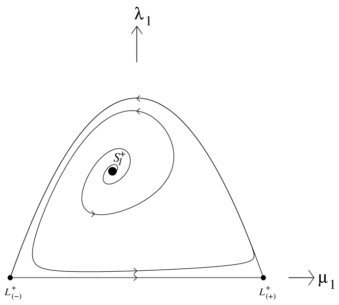
For trajectories confined to the invariant set $\nu_{1}=0$, most trajectories asymptote from the equilibrium point $S^{+}_{1}$ (corresponding to the solution (7.1)) and are future asymptotic to a heteroclinic orbit, consisting of two saddle equilibrium points (which are the points $L^{+}_{(+)}$ and $L^{+}_{(-)}$; i.e., the “$-$” solutions given by equation (6.7) with $h_{0}=\pm\frac{1}{\sqrt{3}}$) and the single boundary orbits in the invariant sets $\lambda_{1}=0$ and $\lambda_{1}+\mu_{1}^{2}=1$. The former set corresponds to a $\Lambda_{\rm M}=0$ solution, whilst the latter to a solution with a constant axion field. The dynamics of this two-dimensional system is of interest from a mathematical point of view due to the existence of the quasi–periodic behaviour. In a given ‘cycle’ an orbit spends a long time close to $L^{+}_{(-)}$ and then moves quickly to $L^{+}_{(+)}$ shadowing the orbit in the invariant set $\lambda_{1}=0$. It is then again quasi-stationary and remains close to the equilibrium point $L^{+}_{(+)}$ before quickly moving back to $L^{+}_{(-)}$ shadowing the orbit in the invariant set $1-\mu_{1}^{2}-\lambda_{1}=0$. It must be stressed that the motion is not periodic, and on each successive cycle a given orbit spends more and more time in the neighbourhood of the equilibrium points $L^{+}_{(+)}$ and $L^{+}_{(-)}$. This qualitative behaviour is quite generic in the following sections whenever $\Lambda_{\rm M}>0$ and $K=0$ and will reappear in sections 8.2.1 and 8.2.2.

Three–Dimensional System ($\dot{\beta}\neq 0$)

Returning to the three–dimensional system (7.17a), the equilibrium sets and their corresponding eigenvalues are

$$S^{+}_{1}: \mu_{1}=-\frac{1}{3\sqrt{3}},\nu_{1}=0,\lambda_{1}=\frac{16}{27};$$ (7.20a)

$$(\lambda_{1},\lambda_{2},\lambda_{3})=\left(\frac{1}{3}+\frac{i\sqrt{231}}{9},\frac{1}{3}-\frac{i\sqrt{231}}{9},\frac{4}{3}\right),$$

$$L^{+}: \nu_{1}=1-\mu_{1}^{2},\lambda_{1}=0;$$ (7.20b)

$$(\lambda_{1},\lambda_{2},\lambda_{3})=\left(-2\sqrt{3}\left[\mu_{1}+\frac{1}{\sqrt{3}}\right],\sqrt{3}\left[\mu_{1}-\frac{1}{\sqrt{3}}\right],0\right).$$

Points on $L^{+}$ with $\mu_{1}^{2}<\frac{1}{3}$ are local sinks, while the equilibrium point $S^{+}_{1}$ is a spiral source. Note that the points $L^{+}_{(\pm)}$ in the two–dimensional system ($\dot{\beta}=0$) are the endpoints to the line $L^{+}$.

Note that in the three–dimensional phase space the variable $\nu_{1}$ is monotonically increasing. When a modulus field is included $(\nu_{1}\neq 0)$, $S^{+}_{1}$ still represents the only source in the system. The orbits follow cyclical trajectories in the neighbourhood of the invariant set $\nu_{1}=0$ and they spiral outwards monotonically, since equation (7.22c) implies that $d\nu_{1}/d\tau>0$. After a finite (but arbitrarily large) number of cycles the kinetic energy of the modulus field becomes more important until a critical point is reached where it dominates the axion and cosmological constant. The orbits then asymptote to the dilaton–moduli–vacuum solutions (6.7). The general behaviour for most trajectories in this phase space is to asymptote away from the equilibrium point $S^{+}_{1}$, spiraling about the line $\mu_{1}=\frac{1}{\sqrt{27}}$, $\nu_{1}=\frac{13}{8}(\lambda_{1}-\frac{16}{27})$ (see (7.3) for this particular line), asymptoting towards the line $L^{+}$ for $\mu_{1}^{2}<\frac{1}{3}$.

Figure 7.2 depicts the full three-dimensional space. Note that the phase diagram depicted in the figure 7.2 is similar to that of figure 1(e) in [188] that describes the locally rotationally symmetric submanifold of the stationary Bianchi type I perfect fluid models in general relativity, although in [188] the independent variable is space-like. Orbits in the full phase space of figure 7.2 with non-trivial modulus field or shear term (represented by the variable $\nu_{1}$) are repelled from the source $S^{+}_{1}$, where $\nu_{1}$ increases monotonically, spiraling around the exact solution given by $\mu_{1}=\frac{1}{\sqrt{27}}$ and $\nu_{1}=\frac{13}{8}(\lambda_{1}-\frac{16}{27})$ (see also equations (7.3)-(7.5)) represented by the dashed line in figure 7.2. This implies that solutions are asymptotic in the past to the solution given by equation (7.1). At early times the orbits ‘shadow’ the orbits in the invariant set $\nu_{1}=0$ and undertake cycles between the saddles (in three-dimensional phase space) on the equilibrium set $L^{+}$ close to $L^{+}_{(-)}$ and $L^{+}_{(+)}$. These saddles on $L^{+}$ may be interpreted as Kasner–like solutions [118, 188]. Note that $\nu_{1}=0$ at $L^{+}_{(+)}$ and $L^{+}_{(-)}$, however, and there is no modulus field or shear term in these cases. The orbits thus experience a finite number of cycles in which the orbits interpolate between different Kasner-like states. The orbits eventually asymptote toward a source on the line $L^{+}$.

Figure 7.2: Phase diagram of the system (7.17a) in the matter sector ($\Lambda_{\rm M}>0$) with $\rho\neq 0$ and $K=0$. Note that $L^{+}$ represents a line of equilibrium points. The invariant set $\dot{\beta}=0$ is depicted in 7.1 on page 7.1. In this phase space, $\psi>0$ is assumed. See also caption to figure 6.1 on page 6.1.

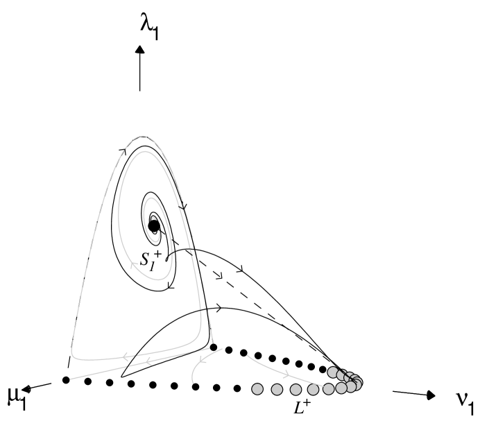
7.3.2 The Case $\Lambda_{\rm M}>0$, $K>0$

For $K>0$, equation (7.11) is written in the new variables as

$$0\leq\mu_{1}^{2}+\nu_{1}+\lambda_{1}\leq 1,\qquad\zeta_{1}+\chi_{1}^{2}=1,$$ (7.21)

where the “$+$” sign is chosen for both $\lambda$ and $\zeta$ in (7.12). For this case, the variable $\zeta_{1}\equiv 1-\chi_{1}^{2}$ will be considered extraneous. The system (7.10a) then reduces to the four-dimensional system:

$$\frac{d\mu_{1}}{d\tau} = \left(1-\!\mu_{1}^{2}-\!\nu_{1}-\!\frac{1}{2}\lambda_{1}\right)\!\left(\sqrt{3}+\!\mu_{1}\chi_{1}\right)-\frac{1}{\sqrt{3}}\left(1-\!\mu_{1}^{2}\right)\!\left(1-\!\chi_{1}^{2}\right)-\sqrt{3}\lambda_{1},$$

$$\frac{d\chi_{1}}{d\tau} = \left(1-\chi_{1}^{2}\right)\left[\mu_{1}^{2}+\nu_{1}+\frac{1}{2}\lambda_{1}+\frac{1}{\sqrt{3}}\mu_{1}\chi_{1}\right],$$ (7.22b)

$$\frac{d\nu_{1}}{d\tau} = \nu_{1}\left[\frac{2}{\sqrt{3}}\mu_{1}\left(1-\chi_{1}^{2}\right)+2\chi_{1}\left(1-\mu_{1}^{2}-\nu_{1}-\frac{1}{2}\lambda_{1}\right)\right],$$ (7.22c)

$$\frac{d\lambda_{1}}{d\tau} = \lambda_{1}\left[\frac{1}{\sqrt{3}}\mu_{1}\left(5-2\chi_{1}^{2}\right)+\chi_{1}\left(1-2\mu_{1}^{2}-2\nu_{1}-\lambda_{1}\right)\right].$$ (7.22d)

The invariant sets $\mu_{1}^{2}+\nu_{1}+\lambda_{1}=1$ ($\rho=0$), $\chi_{1}^{2}=1$ ($K=0$), $\nu_{1}=0$ ($N=0$) and $\lambda_{1}=0$ ($\Lambda_{\rm M}=0$) define the boundaries to the phase space. The equilibrium points and their respective eigenvalues (denoted by $\lambda$) are given by

$$L^{\pm}: \chi_{1}=\pm 1,\mu_{1}^{2}+\nu_{1}=1,\lambda_{1}=0;$$

$$(\lambda_{1},\lambda_{2},\lambda_{3},\lambda_{4})=\left(0,\mp\frac{2}{\sqrt{3}}\left[\sqrt{3}\pm\mu_{1}\right],\sqrt{3}\left[\mu_{1}\mp\frac{1}{\sqrt{3}}\right],\mp 2\sqrt{3}\left[\frac{1}{\sqrt{3}}\pm\mu\right]\right).$$

$$S^{\pm}_{1}: \mu_{1}=\mp\frac{1}{\sqrt{27}},\chi_{1}=\pm 1,\nu_{1}=0,\lambda_{1}=\frac{16}{27};$$ (7.23b)

$$\left(\lambda_{1},\lambda_{2},\lambda_{3},\lambda_{4}\right)=\left(\mp\frac{1}{3}\left[1+i\frac{\sqrt{231}}{3}\right],\mp\frac{1}{3}\left[1-i\frac{\sqrt{231}}{3}\right],\mp\frac{4}{3},\pm\frac{4}{9}\right).$$

From the eigenvalues, it is clear that $L^{+}$ is a late-time attractor for $\mu_{1}^{2}<\frac{1}{3}$, and that $L^{-}$ is an early-time repellor for $\mu_{1}^{2}<\frac{1}{3}$. In both cases, $\chi_{1}^{2}=1$ and therefore $\zeta_{1}=0$ ($K=0$). Both lines represent the dilaton–moduli–vacuum solutions (6.7), and the points $S^{\pm}_{1}$ are saddle points on the boundary of the phase space, corresponding to the exact solutions (7.1).

The Invariant Set $\rho=0$ for $\Lambda_{\rm M}>0$, $K>0$

For the invariant set $\rho=0$, the system (7.3.2) reduces to three dimensions $\{\mu_{1},\chi_{1},\nu_{1}\}$ ($\lambda_{1}=1-\mu_{1}^{2}-\nu_{1}$). The only equilibrium points in this set are the lines $L^{\pm}$ with the first three eigenvalues in (LABEL:Lpm), and therefore the early and time attractors are the lines $L^{-}$ (for $\mu_{1}>-\frac{1}{\sqrt{3}}$) and $L^{+}$ (for $\mu_{1}<\frac{1}{\sqrt{3}}$), respectively. In this invariant set, $\mu$ is a monotonically decreasing function, and so the possibility of periodic orbits is excluded. Therefore, solutions generically asymptote into the past towards the $\dot{\varphi}<0$ dilaton–moduli–vacuum solutions (6.7) for $h_{0}>-\frac{1}{3}$, and asymptote into the future towards the $\dot{\varphi}>0$ dilaton–moduli–vacuum solutions (6.7) for $h_{0}<\frac{1}{3}$. The curvature and cosmological constant are only dynamically significant at intermediate times. The phase space is depicted in figure 7.3.

Figure 7.3: Phase diagram of the system (7.3.2) in the matter ($\Lambda_{\rm M}>0$) sector with $\rho=0$ field and $K>0$. Note that $L^{+}$ and $L^{-}$ represent lines of equilibrium points. See also caption to figure 6.1 on page 6.1.

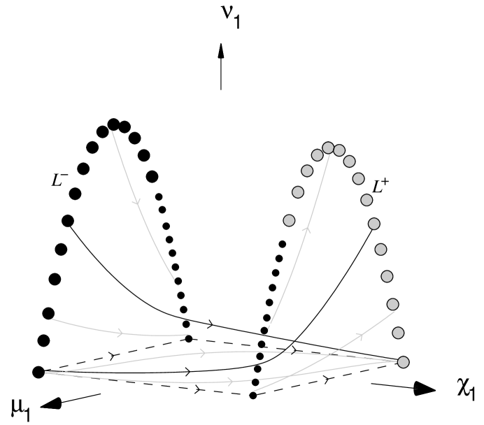
Qualitative Analysis of the Four-Dimensional System

The qualitative dynamics in the full four-dimensional phase space is as follows. The only past–attractors belong to the line $L^{-}$ for $\mu_{1}^{2}<\frac{1}{3}$, and the only future attractors belong to the line $L^{+}$ for $\mu_{1}^{2}<\frac{1}{3}$. Both lines $L^{\pm}$ lie in both invariant sets $\rho=0$ and $\tilde{K}=0$, which is consistent with the analysis of equation (6.15). The function $\chi_{1}\nu_{1}^{\frac{1}{2}}\left(1-\mu_{1}^{2}-\nu_{1}-\lambda_{1}\right)^{\frac{1}{6}}\lambda_{1}^{-\frac{1}{3}}$ monotonically increases and so there can be no periodic orbits. Hence, solutions generically asymptote into the past towards the $\dot{\varphi}<0$ dilaton–moduli–vacuum solutions (6.7) for $h_{0}^{2}<\frac{1}{9}$, and into the future towards the $\dot{\varphi}>0$ dilaton–moduli–vacuum solutions (6.7) for $h_{0}^{2}<\frac{1}{9}$. The curvature, cosmological constant term and the axion field are only dynamically significant at intermediate times.

For orbits in the four-dimensional phase space, the complex eigenvalues of the saddle point $S^{\pm}_{1}$ suggest that the heteroclinic sequences may exist in the four–dimensional set. Indeed, those orbits which asymptote to the $\tilde{K}=0$ invariant set do generically spend time in a heteroclinic sequence, interpolating between two equilibrium points representing two dilaton–vacuum solutions, as discussed in subsection 7.3.1. However, for those orbits which asymptote towards the $\rho=0$ invariant set, there are no heteroclinic sequences (as is evident from figure 7.3), and asymptote to equilibrium points representing dilaton–moduli–vacuum solutions.

7.3.3 The Case $\Lambda_{\rm M}>0$, $K<0$

For $K<0$, equation (7.11) is written in the new variables as

$$0\leq\mu_{2}^{2}+\nu_{2}+\zeta_{2}+\lambda_{2}\leq 1,\qquad\chi_{2}^{2}=1,$$ (7.24)

where the “$+$” sign for $\lambda$ and the “$-$” sign for $\zeta$ has been chosen in (7.12). For this case, $\chi_{2}=+1$ is explicitly chosen, as $\chi_{2}=-1$ corresponds to a time reversal of (7.10a). The system (7.10a) then reduces to the four-dimensional system:

$$\frac{d\mu_{2}}{d\tau} = \left(1-\mu_{2}^{2}-\nu_{2}-\frac{1}{2}\lambda_{2}\right)\left(\sqrt{3}+\mu_{2}\right)-\sqrt{3}\left(\lambda_{2}+\frac{2}{3}\zeta_{2}\right),$$ (7.25a)

$$\frac{d\nu_{2}}{d\tau} = 2\nu_{2}\left(1-\mu_{2}^{2}-\nu_{2}-\frac{1}{2}\lambda_{2}\right),$$ (7.25b)

$$\frac{d\zeta_{2}}{d\tau} = -2\zeta_{2}\left(\mu_{2}^{2}+\nu_{2}+\frac{1}{2}\lambda_{2}+\frac{1}{\sqrt{3}}\mu_{2}\right),$$ (7.25c)

$$\frac{d\lambda_{2}}{d\tau} = \lambda_{2}\left(1-2\mu_{2}^{2}-2\nu_{2}-\lambda_{2}+\sqrt{3}\mu_{2}\right).$$ (7.25d)

The invariant sets $\mu_{2}^{2}+\nu_{2}+\zeta_{2}+\lambda_{2}=1$ ($\rho=0$), $\zeta_{2}=0$ ($K=0$), $\nu_{1}=0$ ($N=0$) and $\lambda_{1}=0$ ($\Lambda_{\rm M}=0$) define the boundaries to the phase space. The equilibrium points and their respective eigenvalues (denoted by $\lambda$) are given by

$$S^{+}: \mu_{2}=-\frac{1}{\sqrt{3}},\zeta_{2}=\frac{2}{3},\lambda_{2}=0,\nu_{2}=0;$$ (7.26a)

$$(\lambda_{1},\lambda_{2},\lambda_{3},\lambda_{4})=\frac{1}{3}(2,4,-2,4),$$

$$N: \mu_{2}=-\frac{\sqrt{3}}{5},\nu_{2}=0,\zeta_{2}=\frac{18}{25},\lambda_{2}=\frac{4}{25};$$ (7.26b)

$$(\lambda_{1},\lambda_{2},\lambda_{3},\lambda_{4})=\frac{2}{5}(1+i\sqrt{2},1-i\sqrt{2},4,2),$$

$$L^{+}: \mu_{2}^{2}+\nu_{2}=1,\zeta_{2}=0,\lambda_{2}=0;$$

$$(\lambda_{1},\lambda_{2},\lambda_{3},\lambda_{4})=\left(0,-\frac{2}{\sqrt{3}}\left[\mu_{2}+\sqrt{3}\right],\sqrt{3}\left[\mu_{2}-\frac{1}{\sqrt{3}}\right],-2\sqrt{3}\left[\mu_{2}+\frac{1}{\sqrt{3}}\right]\right).$$

From the eigenvalues, it is clear that $L^{+}$ is a late-time attractor for $\mu_{1}^{2}<\frac{1}{3}$. This line represents the dilaton–moduli–vacuum solutions (6.7). The point $N$ inside the phase space is the early-time attractor for the system, and represents the curvature–driven, static–modulus, static–axion solution (7.1). The saddle point $S^{+}$ corresponds to the Milne model (6.9).

The Invariant Set $\rho=0$ for $\Lambda_{\rm M}>0$, $K<0$

For this invariant set, the four–dimensional system (7.25a) reduces to a three–dimensional system involving the coordinates $\{\mu_{2},\nu_{2},\lambda_{2}\}$ ($\zeta_{2}=1-\mu_{2}^{2}-\nu_{2}-\lambda_{2}$). The equilibrium points are the same as the full four-dimensional set, but with eigenvalues ($\lambda_{1},\lambda_{2},\lambda_{3}$), and so the line $L^{+}$ is a sink for $\mu_{2}<\frac{1}{\sqrt{3}}$, and $N$ is a source. The variable $\nu$ is a monotonically increasing function, the existence of which eliminates the possibility for recurrent orbits to occur. Therefore, the generic behaviour of this model is for solutions to asymptote into the past towards the curvature–dominated, static–modulus, static–axion solution (7.1), and to the future towards the $\dot{\varphi}>0$ dilaton–moduli–vacuum solutions (6.7) for $h_{0}<\frac{1}{3}$. Figure 7.4 depicts this phase space.

Figure 7.4: Phase diagram of the system (7.25a) in the matter ($\Lambda_{\rm M}>0$) sector with $\rho=0$ and $K<0$. Note that $L^{+}$ represents a line of equilibrium points. In this phase space, $\psi>0$ is assumed. See also caption to figure 6.1 on page 6.1.

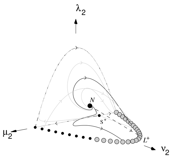
Qualitative Analysis of the Four-Dimensional System

In the full four-dimensional set, the point $N$ is the early-time attractor, and $L^{+}$ is the late-time attractor for $\mu_{2}^{2}<\frac{1}{3}$. The point $N$ lies in the invariant set $\rho=0$ and $L^{+}$ lies in both the invariant sets $\rho=0$ and $\tilde{K}=0$, which is consistent with the analysis of equation (6.15). It is apparent that $\nu_{2}$ is a monotonically increasing function, and so the possibility of recurrent or periodic orbits is not allowed. Therefore, generically, solutions asymptote into the past towards the curvature–dominated, static–modulus, static–axion solution (7.1), and into the future towards the $\dot{\varphi}>0$ dilaton–moduli–vacuum solutions (6.7) for $h_{0}^{2}<\frac{1}{9}$. Since, $\nu$ monotonically increases, the modulus field is initially dynamically trivial, but becomes dynamically significant asymptotically into the future. The axion field and the cosmological constant are dynamically significant only at intermediate times and do not play a rôle in the early- and late-time dynamical evolution. The curvature term is dynamically significant at early and intermediate times, but becomes dynamically trivial at late times.

Orbits which asymptote into the future towards the $K=0$ invariant set, generically end in a heteroclinic sequence as described in section 4.1.1 and depicted in figure 7.2. However, such a sequence does not occur for orbits which asymptote into the future towards the $\rho=0$ invariant set. Indeed, by examining the eigenvalues of the equilibrium points of the four-dimensional system, there do not seem to be heteroclinic sequences outside of the $\tilde{K}=0$ invariant set.

For mathematical completeness, the $\Lambda_{\rm M}<0$ cases will now be studied.

7.3.4 The Case $\Lambda_{\rm M}<0$, $K=0$

For this case, equation (7.11) is written in the new variables as

$$0\leq\mu_{3}^{2}+\nu_{3}\leq 1,\qquad\chi_{3}^{2}+\lambda_{3}=1,$$ (7.27)

where the “$-$” sign for $\lambda$ has been chosen in (7.12). The variable $\lambda_{3}$ is chosen as the extraneous variable and the system (7.10a) then reduces to the four-dimensional system:

$$\frac{d\mu_{3}}{d\tau} = \frac{\sqrt{3}}{2}\left(1-\mu_{3}^{2}\right)\left(1-\chi_{3}^{2}\right)+\left(1-\mu_{3}^{2}-\nu_{3}\right)\left(\sqrt{3}+\mu_{3}\chi_{3}\right),$$ (7.28a)

$$\frac{d\chi_{3}}{d\tau} = -\frac{1}{2}\left(1-\chi_{3}^{2}\right)\left(1-2\mu_{3}^{2}-2\nu_{3}+\sqrt{3}\mu_{3}\chi_{3}\right),$$ (7.28b)

$$\frac{d\nu_{3}}{d\tau} = \nu_{3}\left[2\chi_{3}\left(1-\mu_{3}^{2}-\nu_{3}\right)-\sqrt{3}\mu_{3}\left(1-\chi_{3}^{2}\right)\right].$$ (7.28c)

The phase space is bounded by the sets $\chi_{3}=\pm 1$ and $\nu_{3}=1-\mu_{3}^{2}$, where the latter corresponds to a zero axion field. The dynamics is determined by the fact that the right-hand side of equation (7.28a) is positive definite so that $\mu_{3}$ is a monotonically increasing function.

The Frozen Modulus ($\dot{\beta}=0$) Invariant Set

The invariant set $\dot{\beta}=0$, corresponding to $\nu_{3}$, is first examined. For this case, the dynamical system becomes equations (7.28a) and (7.28b) with $\nu_{3}=0$, and the equilibrium points (and their eigenvalues) are given by

$$L^{+}_{(+)}: \chi_{3}=1,\mu_{3}=1;$$ (7.29a)

$$(\lambda_{1},\lambda_{2})=\left(\sqrt{3}\left[1-\frac{1}{\sqrt{3}}\right],-2\sqrt{3}\left[1+\frac{1}{\sqrt{3}}\right]\right),$$

$$L^{+}_{(-)}: \chi_{3}=1,\mu_{3}=-1;$$ (7.29b)

$$(\lambda_{1},\lambda_{2})=\left(-\sqrt{3}\left[1+\frac{1}{\sqrt{3}}\right],2\sqrt{3}\left[1+\frac{1}{\sqrt{3}}\right]\right),$$

$$L^{-}_{(+)}: \chi_{3}=-1,\mu_{3}=1;$$ (7.29c)

$$(\lambda_{1},\lambda_{2})=\left(\sqrt{3}\left[1+\frac{1}{\sqrt{3}}\right],-2\sqrt{3}\left[1-\frac{1}{\sqrt{3}}\right]\right),$$

$$L^{-}_{(-)}: \chi_{3}=-1,\mu_{3}=-1;$$ (7.29d)

$$(\lambda_{1},\lambda_{2})=\left(-\sqrt{3}\left[1-\frac{1}{\sqrt{3}}\right],2\sqrt{3}\left[1+\frac{1}{\sqrt{3}}\right]\right),$$

$$R: \chi_{3}=-\frac{1}{\sqrt{3}},\mu_{3}=-1,\nu_{3}=0;$$ (7.29e)

$$(\lambda_{1},\lambda_{2})=\frac{1}{\sqrt{3}}\left(1,10\right),$$

$$A: \chi_{3}=\frac{1}{\sqrt{3}},\mu_{3}=1,\nu_{3}=0;$$ (7.29f)

$$(\lambda_{1},\lambda_{2})=-\frac{1}{\sqrt{3}}\left(1,10\right).$$

The four points $L^{\pm}_{(\pm)}$ are saddles, whereas the point $R$ is a source and the point $A$ is a sink. Figure 7.5 depicts this phase space.

Figure 7.5: Phase diagram of the system (7.28a) in the matter ($\Lambda_{\rm M}<0$) sector with $K=0$ and $\dot{\beta}=0$. See also caption to figure 6.1 on page 6.1.

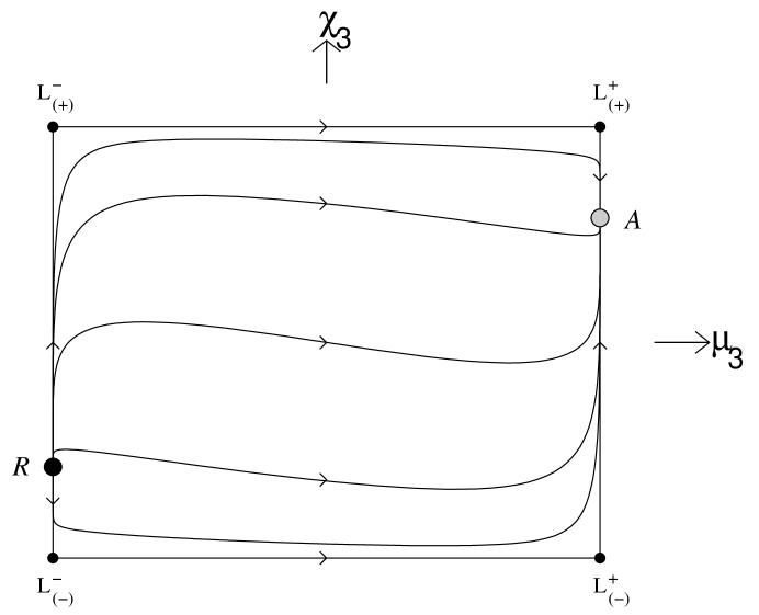
Three–Dimensional System ($\dot{\beta}\neq 0$)

Returning to the three–dimensional system (7.28a), the equilibrium points and their respective eigenvalues are:

$$L^{\pm}: \chi_{3}=\pm 1,\mu_{3}^{2}+\nu_{3}=1;$$ (7.30a)

$$(\lambda_{1},\lambda_{2},\lambda_{3})=\left(0,\sqrt{3}\left[\mu_{3}\mp\frac{1}{\sqrt{3}}\right],-2\sqrt{3}\left[\mu_{3}\pm\frac{1}{\sqrt{3}}\right]\right),$$

$$R: \chi_{3}=-\frac{1}{\sqrt{3}},\mu_{3}=-1,\nu_{3}=0;$$ (7.30b)

$$(\lambda_{1},\lambda_{2},\lambda_{3})=\frac{1}{\sqrt{3}}\left(1,2,10\right),$$

$$A: \chi_{3}=\frac{1}{\sqrt{3}},\mu_{3}=1,\nu_{3}=0;$$ (7.30c)

$$(\lambda_{1},\lambda_{2},\lambda_{3})=-\frac{1}{\sqrt{3}}\left(1,2,10\right).$$

Note that the points $L^{+}_{(+)}$ and $L^{+}_{(-)}$ from the two–dimensional system ($\dot{\beta}=0$) are the endpoints to the line $L^{+}$ whereas the points $L^{-}_{(+)}$ and $L^{-}_{(-)}$ are the endpoints to the line $L^{-}$. The line $L^{-}$ represents early–time attracting solutions for $\mu_{3}^{2}<\frac{1}{3}$ and saddles otherwise. The saddle points The line $L^{+}$ corresponds to late–time attracting solutions for $\mu_{3}^{2}<\frac{1}{3}$ and saddles otherwise. Hence, there are two early–time attractors given by the point $R$ and the line $L^{-}$ for $\mu_{3}^{2}<\frac{1}{3}$. There are also two late–time attractors corresponding to the point $A$ and the line $L^{+}$ for $\mu_{3}^{2}<\frac{1}{3}$. Figure 7.6 depicts this phase space.

Figure 7.6: Phase diagram of the system (7.28a) in the matter ($\Lambda_{\rm M}<0$) sector with $\rho\neq 0$ and $K=0$. Note that $L^{+}$ and $L^{-}$ represent lines of equilibrium points. The invariant set $\nu_{3}=0$ is depicted in figure 7.5 on page 7.5. See also caption to figure 6.1 on page 6.1.

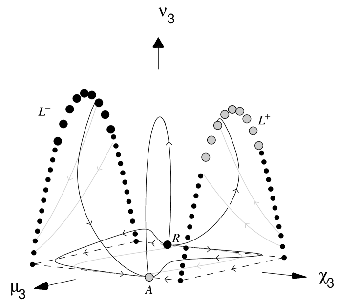
Because $\mu_{3}$ monotonically increases, most trajectories in this phase space represent bouncing cosmologies which are initially contracting and end up expanding. Most trajectories asymptote into the past towards either $L^{-}$, representing the $\dot{\varphi}<0$ dilaton–moduli–vacuum solutions (6.7), or to $R$, representing the static-moduli solution (7.8). To the future, most orbits asymptote towards either $L^{+}$, representing the $\dot{\varphi}>0$ dilaton–moduli–vacuum solutions, or $A$ corresponding to the expanding, static-moduli solution.

7.3.5 The Case $\Lambda_{\rm M}<0$, $K>0$

For this case, equation (7.11) is written in the new variables as

$$0\leq\mu_{3}^{2}+\nu_{3}\leq 1,\qquad\chi_{3}^{2}+\zeta_{3}+\lambda_{3}=1,$$ (7.31)

where the “$-$” sign for $\lambda$ and the “$+$” sign for $\zeta$ has been chosen in (7.12). The variable $\lambda_{3}$ is chosen as the extraneous variable and the system (7.10a) then reduces to the four-dimensional system:

$$\frac{d\mu_{3}}{d\tau} = \left(1-\mu_{3}^{2}-\nu_{3}\right)\left(\sqrt{3}+\mu_{3}\chi_{3}\right)+\frac{\sqrt{3}}{2}\left(1-\mu_{3}^{2}\right)\left(1-\chi_{3}^{2}-\frac{5}{3}\zeta_{3}\right),$$ (7.32a)

$$\frac{d\chi_{3}}{d\tau} = -\frac{\sqrt{3}}{2}\left[\mu_{3}\chi_{3}\left(1-\chi_{3}^{2}-\frac{5}{3}\zeta_{3}\right)\right]-\frac{1}{2}\left(1-\chi_{3}^{2}\right)\left(1-2\mu_{3}^{2}-2\nu_{3}\right)+\frac{1}{2}\zeta_{3},$$

$$\frac{d\nu_{3}}{d\tau} = \nu_{3}\left[2\chi_{3}\left(1-\mu_{3}^{2}-\nu_{3}\right)-\sqrt{3}\mu_{3}\left(1-\chi_{3}^{2}-\frac{5}{3}\zeta_{3}\right)\right],$$ (7.32c)

$$\frac{d\zeta_{3}}{d\tau} = -\zeta_{3}\left[2\chi_{3}\left(\mu_{3}^{2}+\nu_{3}\right)+\frac{1}{\sqrt{3}}\mu_{3}\left(5-3\chi_{3}^{2}-5\zeta_{3}\right)\right].$$ (7.32d)

The invariant sets $\mu_{3}^{2}+\nu_{3}=1$, $\chi_{3}^{2}+\zeta_{3}=1$, $\nu_{3}=0$ and $\zeta_{3}=0$ define the boundary of the phase space.

The equilibrium sets and their corresponding eigenvalues (denoted by $\lambda$) are

$$L^{\pm}: \chi_{3}=\pm 1,\mu_{3}^{2}+\nu_{3}=1,\zeta_{3}=0;$$

$$(\lambda_{1},\lambda_{2},\lambda_{3},\lambda_{4})=\left(0,\mp\frac{2}{\sqrt{3}}\left[\sqrt{3}\pm\mu_{3}\right],\sqrt{3}\left[\mu_{3}\mp\frac{1}{\sqrt{3}}\right],-2\sqrt{3}\left[\mu_{3}\pm\frac{1}{\sqrt{3}}\right]\right),$$

$$R: \chi_{3}=-\frac{1}{\sqrt{3}},\mu_{3}=-1,\nu_{3}=0,\zeta_{3}=0;$$ (7.33b)

$$(\lambda_{1},\lambda_{2},\lambda_{3},\lambda_{4})=\frac{1}{\sqrt{3}}\left(1,2,6,10\right),$$

$$A: \chi_{3}=\frac{1}{\sqrt{3}},\mu_{3}=1,\nu_{3}=0,\zeta_{3}=0;$$ (7.33c)

$$(\lambda_{1},\lambda_{2},\lambda_{3},\lambda_{4})=-\frac{1}{\sqrt{3}}\left(1,2,6,10\right).$$

Here there are two early-time attractors: the point $R$ representing the $\dot{\varphi}<0$ static–modulus, static–axion solution (7.8) and the line $L^{-}$ for $\mu_{3}^{2}<\frac{1}{3}$. Likewise, there are two late-time attractors: the point $A$ representing the $\dot{\varphi}>0$ static–modulus, static–axion solution (7.8) and the line $L^{+}$ for $\mu_{3}^{2}<\frac{1}{3}$.

The Invariant Set $\rho=0$ for $\Lambda_{\rm M}<0$, $K>0$

For this invariant set, the four-dimensional system (7.32a) reduces to a three-dimensional system involving the coordinates $\{\mu_{3},\chi_{3},\zeta_{3}\}$ ($\nu_{3}=1-\mu_{2}^{3}$). The equilibrium points are the same as the full four-dimensional set, but with eigenvalues ($\lambda_{1},\lambda_{2},\lambda_{3}$), and so the line $L^{-}$ is a source for $\mu_{3}>-\frac{1}{\sqrt{3}}$ and the line $L^{+}$ is a sink for $\mu_{3}<\frac{1}{\sqrt{3}}$. The function $\chi_{3}/\sqrt{\nu_{3}}$ is monotonically increasing, and so there are no recurring or periodic orbits. Hence, solutions generically asymptote into the past towards either the $\dot{\varphi}<0$ dilaton–moduli–vacuum solutions (6.7) for $h_{0}>-\frac{1}{3}$, or the contracting $\dot{\varphi}<0$ static–modulus, static–axion solution (7.8), represented by $R$. Into the future, solutions asymptote towards either the expanding $\dot{\varphi}>0$ dilaton–moduli–vacuum solutions (6.7) for $h_{0}<\frac{1}{3}$, or the $\dot{\varphi}>0$ static–modulus, static–axion solution (7.8), represented by $A$. Figure 7.7 depicts this phase space.

Figure 7.7: Phase diagram of the system (7.32a) in the matter ($\Lambda_{\rm M}<0$) sector with $\rho=0$ and $K>0$. Note that $L^{+}$ and $L^{-}$ represent lines of equilibrium points. See also caption to figure 6.1 on page 6.1.

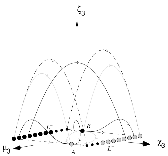
Qualitative Analysis of the Four-Dimensional System

In the full four-dimensional set, the early-time attractors are the line $L^{-}$ for $\mu_{3}^{2}<\frac{1}{3}$ and the point $R$. The late-time attractors are the $L^{+}$ for $\mu_{3}^{2}<\frac{1}{3}$ and the point $A$. All of these attractors lie in both of the invariant sets $\rho=0$ and $\tilde{K}=0$, which is consistent with the analysis of (6.15). The function $\left(\chi_{3}+\frac{1}{\sqrt{3}}\mu_{3}\right)/\sqrt{\nu_{3}}$ is monotonically increasing, and so there are no recurring or periodic orbits. Hence, solutions generically asymptote into the past towards either the $\dot{\varphi}<0$ dilaton–moduli–vacuum solutions (6.7) for $h_{0}^{2}<\frac{1}{9}$, or the inflating $\dot{\varphi}<0$ static–modulus, static–axion solution (7.8). Into the future, solutions asymptote towards either the $\dot{\varphi}>0$ dilaton–moduli–vacuum solutions (6.7) for $h_{0}^{2}<\frac{1}{9}$, or the $\dot{\varphi}>0$ static–modulus, static–axion solution (7.8). The axion field and curvature term are dynamically significant only at intermediate times. For early and late times, the cosmological constant is dynamically significant only when the modulus field is dynamically trivial (e.g., the points $R$ and $A$) and vice-versa (e.g., the lines $L^{\pm}$).

7.3.6 The Case $\Lambda_{\rm M}<0$, $K<0$

For this case, equation (7.11) is written in the new variables as

$$0\leq\mu_{4}^{2}+\nu_{4}+\zeta_{4}\leq 1,\qquad\chi_{4}^{2}+\lambda_{4}=1,$$ (7.34)

where the “$-$” sign for both $\lambda$ and $\zeta$ has been chosen in (7.12). The variable $\lambda_{4}$ is chosen as the extraneous variable and the system (7.10a) then reduces to the four-dimensional system:

$$\frac{d\mu_{4}}{d\tau} = \left(1-\mu_{4}^{2}-\nu_{4}\right)\left(\sqrt{3}+\mu_{4}\chi_{4}\right)+\frac{\sqrt{3}}{2}\left(1-\mu_{4}^{2}\right)\left(1-\chi_{4}^{2}\right)-\frac{2}{\sqrt{3}}\zeta_{4},$$ (7.35a)

$$\frac{d\chi_{4}}{d\tau} = -\frac{1}{2}\left(1-\chi_{4}^{2}\right)\left[1-2\mu_{4}^{2}-2\nu_{4}+\sqrt{3}\mu_{4}\chi_{4}\right],$$ (7.35b)

$$\frac{d\nu_{4}}{d\tau} = \nu_{4}\left[2\chi_{4}\left(1-\mu_{4}^{2}-\nu_{4}\right)-\sqrt{3}\mu_{4}\left(1-\chi_{4}^{2}\right)\right],$$ (7.35c)

$$\frac{d\zeta_{4}}{d\tau} = -\zeta_{4}\left[2\chi_{4}\left(\mu_{4}^{2}+\nu_{4}\right)+\frac{1}{\sqrt{3}}\mu_{4}\left(5-3\chi_{4}^{2}\right)\right].$$ (7.35d)

The invariant sets $\mu_{4}^{2}+\nu_{4}+\zeta_{4}=1$, $\chi_{4}^{2}=1$, $\nu_{4}=0$ and $\zeta_{4}=0$ define the boundary to the phase space. The equilibrium sets and their corresponding eigenvalues (denoted by $\lambda$) are

$$L^{\pm}: \chi_{4}=\pm 1,\mu_{4}^{2}+\nu_{4}=1,\zeta_{4}=0;$$

$$(\lambda_{1},\lambda_{2},\lambda_{3},\lambda_{4})=\left(0,\mp\frac{2}{\sqrt{3}}\left[\sqrt{3}\pm\mu_{4}\right],\sqrt{3}\left[\mu_{4}\mp\frac{1}{\sqrt{3}}\right],-2\sqrt{3}\left[\mu_{4}\pm\frac{1}{\sqrt{3}}\right]\right),$$

$$R: \chi_{4}=-\frac{1}{\sqrt{3}},\mu_{4}=-1,\nu_{4}=0,\zeta_{4}=0;$$ (7.36b)

$$(\lambda_{1},\lambda_{2},\lambda_{3},\lambda_{4})=\frac{1}{\sqrt{3}}\left(1,2,6,10\right),$$

$$A: \chi_{4}=\frac{1}{\sqrt{3}},\mu_{4}=1,\nu_{4}=0,\zeta_{4}=0;$$ (7.36c)

$$(\lambda_{1},\lambda_{2},\lambda_{3},\lambda_{4})=-\frac{1}{\sqrt{3}}\left(1,2,6,10\right),$$

$$S^{\pm} \chi_{4}=\pm 1,\mu_{4}=\frac{\mp 1}{\sqrt{3}},\nu_{4}=0,\zeta_{4}=\frac{2}{3};$$ (7.36d)

$$(\lambda_{1},\lambda_{2},\lambda_{3},\lambda_{4})=\frac{2}{3}(\mp 1,\pm 1,\pm 2,0).$$

As in the previous case, there are two early-time attractors: the point $R$ (corresponding to the $\dot{\varphi}<0$ static–modulus, static–axion solution (7.8)) and the line $L^{-}$ for $\mu_{4}^{2}<\frac{1}{3}$ (corresponding to (6.7) for $h_{0}^{2}<\frac{1}{9}$). Likewise, there are two late-time attractors: the point $A$ (corresponding to the $\dot{\varphi}>0$ static–modulus, static–axion solution (7.8)) and the line $L^{+}$ for $\mu_{4}^{2}<\frac{1}{3}$ (corresponding to (6.7) for $h_{0}^{2}<\frac{1}{9}$).

The Invariant Set $\rho=0$ for $\Lambda_{\rm M}<0$, $K<0$

For this invariant set, the four-dimensional system (7.35a) reduces to a three-dimensional system involving the coordinates $\{\mu_{4},\chi_{4},\nu_{4}\}$ ($\zeta_{4}=1-\mu_{4}^{3}-\nu_{4}$). The equilibrium points are the same as the full four-dimensional set, but with eigenvalues ($\lambda_{1},\lambda_{2},\lambda_{3}$), except now the line $L^{+}$ is a sink for $\mu_{4}<\frac{1}{\sqrt{3}}$ and the line $L^{-}$ is a source for $\mu_{4}>-\frac{1}{\sqrt{3}}$. The function $\mu_{4}/\sqrt{\nu_{4}}$ is monotonically increasing, and so it is not possible for periodic orbits to occur. Hence, solutions generically asymptote into the past towards either the $\dot{\varphi}<0$ dilaton–moduli–vacuum solutions (6.7) for $h_{0}>-\frac{1}{3}$, or the contracting $\dot{\varphi}<0$ static–modulus, static–axion solution (7.8). Into the future, solutions asymptote towards either the $\dot{\varphi}>0$ dilaton–moduli–vacuum solutions (6.7) for $h_{0}<\frac{1}{3}$, or the expanding $\dot{\varphi}>0$ static–modulus, static–axion solution (7.8). Figure 7.8 depicts this phase space.

Figure 7.8: Phase diagram of the system (7.35a) in the matter ($\Lambda_{\rm M}<0$) sector with $\rho=0$ and $K<0$. Note that $L^{+}$ and $L^{-}$ represent line of equilibrium points. See also caption to figure 6.1 on page 6.1.

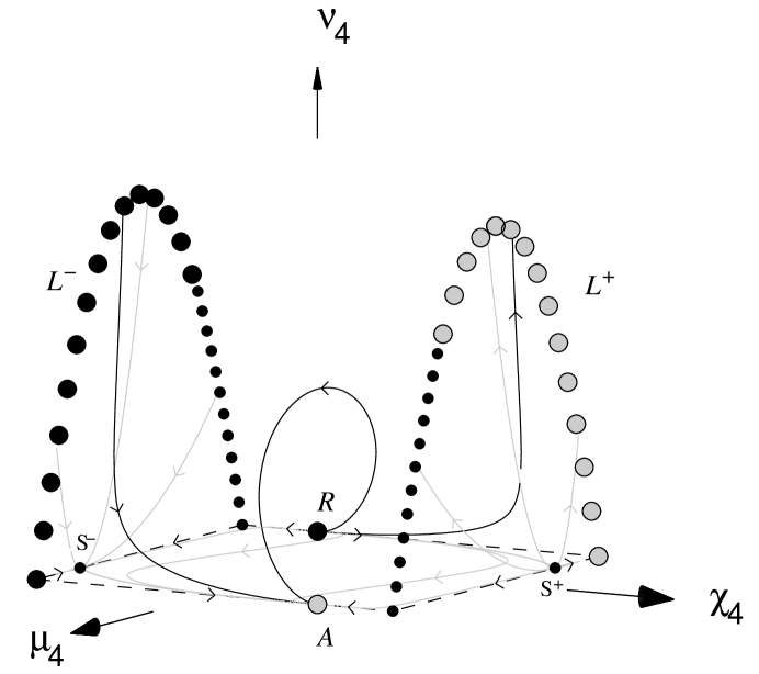
Qualitative Analysis of the Four-Dimensional System

The invariant set $K=0$ is discussed in subsection 7.3.6 (see figure 7.6).

In the full four-dimensional set, the early-time attractors are the line $L^{-}$ for $\mu_{4}^{2}<\frac{1}{3}$ and the point $R$. The late-time attractors are the $L^{+}$ for $\mu_{3}^{2}<\frac{1}{3}$ and the point $A$. All of these attractors lie in both of the invariant sets $\rho=0$ and $\tilde{K}=0$, which is consistent with the analysis of (6.15). The function $\mu_{4}/\sqrt{\nu_{4}}$ is monotonically increasing, and so there are no recurring or periodic orbits. Hence, solutions generically asymptote into the past towards either the $\dot{\varphi}<0$ dilaton–moduli–vacuum solutions (6.7) for $h_{0}^{2}<\frac{1}{9}$ (corresponding to $L^{-}$), or the contracting $\dot{\varphi}<0$ static–modulus, static–axion solution (7.8) (represented by $R$). Into the future, solutions asymptote towards either the $\dot{\varphi}>0$ dilaton–moduli–vacuum solutions (6.7) for $h_{0}^{2}<\frac{1}{9}$ (corresponding to $L^{+}$) or the expanding $\dot{\varphi}>0$ static–modulus, static–axion solution (7.8) (represented by $A$). The axion field and curvature term are dynamically significant only at intermediate times. For early and late times, the cosmological constant is dynamically significant only when the modulus field is dynamically trivial (e.g., the points $R$ and $A$) and vice-versa (e.g., the lines $L^{\pm}$).

7.4 Summary of Analysis in the Jordan Frame

This discussion begins with two tables; Table 7.1 lists which terms are the dominant variables for each equilibrium set as well as the deceleration parameter, $q$, for the corresponding model and Table 7.2 lists the attracting behaviour of the equilibrium sets.

Set	Dominant Variables								$q$	H
$L^{+}$ ($t<0$)	$\alpha$	$\hat{\Phi}$	$\dot{\beta}$						$-(1+h_{0})h_{0}^{-1}$	$h_{0}(-t)^{-1}$
$L^{-}$ ($t>0$)	$\alpha$	$\hat{\Phi}$	$\dot{\beta}$						$(1-h_{0})h_{0}^{-1}$	$h_{0}t^{-1}$
$S_{1}^{+}$ ($t<0$)	$\alpha$	$\hat{\Phi}$		$\dot{\sigma}$			$\Lambda_{\rm M}>0$		$2$	$\frac{1}{3}t^{-1}$
$S_{1}^{-}$ ($t>0$)	$\alpha$	$\hat{\Phi}$		$\dot{\sigma}$			$\Lambda_{\rm M}>0$		$2$	$\frac{1}{3}t^{-1}$
$A$ ($t<0$)	$\alpha$	$\hat{\Phi}$					$\Lambda_{\rm M}<0$		$-3$	$-\frac{1}{2}t^{-1}$
$R$ ($t>0$)	$\alpha$	$\hat{\Phi}$					$\Lambda_{\rm M}<0$		$-3$	$-\frac{1}{2}t^{-1}$
$N$ ($t<0$)	$\alpha$	$\hat{\Phi}$			$k<0$		$\Lambda_{\rm M}>0$		$0$	$t^{-1}$
$S^{\pm}$	$\alpha$				$k<0$				$0$	$t^{-1}$

Table 7.1: The dominant variables for each equilibrium set as well as the equilibrium set’s deceleration parameter, $q$, and Hubble parameter $H$. Inflation occurs when $q<0$ and $H>0$, whereas “deflation” occurs for $q>0$ and $H<0$. Note that the only “anisotropic” solutions are represented by the lines $L^{\pm}$, except when $h_{0}^{2}=\frac{1}{3}$.

Note that the only inflationary models are those represented by $L^{+}$ (for $h_{0}>0$) and $A$. The saddle point $S^{+}_{1}$ represents a deflating model ($q>0$, $H<0$).

Terms Present					Early	Intermediate	Late
$\dot{\beta}$			$\Lambda_{\rm M}>0$		$S^{+}_{1}$	$L^{+}$	$L^{+}$
$\dot{\beta}$	$k>0$		$\Lambda_{\rm M}>0$		$L^{-}$	$S^{\pm}_{1}$, $L^{\pm}$	$L^{+}$
$\dot{\beta}$	$k<0$		$\Lambda_{\rm M}>0$		$N$	$S^{+}$, $L^{+}$	$L^{+}$
$\dot{\beta}$	$k$		$\Lambda_{\rm M}<0$		$R$, $L^{-}$	$L^{\pm}$	$A$, $L^{+}$

Table 7.2: Summary of the early-time, intermediate, and late-time attractors for the various models examined. Note that $\dot{\alpha}$, $\hat{\Phi}$ and $\dot{\sigma}$ are present in every model.

Monotonic functions have been established for each case, which precludes the existence of recurrent or periodic orbits and thereby allowing the early-time and late-time behaviour of these models to be determined based upon the equilibrium sets of the system. In all cases, the dilaton–moduli–vacuum solutions act as either early-time or late-time attractors (and, in many of the cases, both). Because these solutions lie in both the $\rho=0$ and $\tilde{K}=0$ invariant sets and contain no cosmological constant, and therefore the modulus and dilaton fields are dynamically important asymptotically. Furthermore, all early-time and late-time attracting sets lie in either the $\rho=0$ invariant set, or the $\tilde{K}=0$ invariant set, and a majority of these sets lie in both; thus, there seems to be a generic feature in which the curvature terms and the axion field are dynamically significant at intermediate times and are asymptotically negligible at early and at late times.

When $\Lambda_{\rm M}>0$, the cosmological constant may play a significant rôle in the early and late time dynamics. For instance, although in the four-dimensional sets there are no repelling or attracting equilibrium points in which $\Lambda_{\rm M}$ is dynamically significant, the orbits which are attracted to the $\tilde{K}=0$ invariant can spend some time in a heteroclinic sequence which interpolates between two dilaton–moduli–vacuum solutions (see subsection 7.3.1, figure 7.2). During this interpolation, the orbits repeatedly spend time in a region of phase space in which $\Lambda_{\rm M}$ is dynamically significant (the region $\lambda_{1}>0$ in figure 7.2), although most time is spend near the dilaton–moduli–vacuum saddle points where $\Lambda_{\rm M}$ is dynamically negligible. When $\Lambda_{\rm M}<0$, the cosmological constant can be dynamically significant at both early times and at late times, since solutions can typically asymptote to static–modulus, static–axion solutions (7.8) (as well as asymptoting to the dilaton–moduli–vacuum solutions). For the repelling and attracting sets of the $\Lambda_{\rm M}<0$ cases, the modulus field is only dynamically significant when the cosmological constant is not, and vice versa.

Typically, the curvature term is found to be be dynamically significant only at intermediate times, and is asymptotically negligible. However, the only exceptions to this is the case $\Lambda_{\rm M}>0$, $\tilde{K}<0$ in which the repellor $N$ represents the curvature–driven, static–modulus, static–axion solution (7.1). Finally, cases in which $\Lambda_{\rm M}>0$ there exist heteroclinic sequences in the invariant set $\tilde{K}=0$; this implies that the qualitative behaviour associated with heteroclinic sequences described is only valid for solutions which approach $\tilde{K}=0$.

The only anisotropic models are the dilaton–moduli-vacuum solutions (6.7). These solutions are attracting solutions (either into the past or future) for most models. However, these are not the only asymptotic solutions and all other solutions mentioned in this chapter are isotropic ($\dot{\beta}=0$). In particular, the models in which $\Lambda_{\rm M}<0$ do have isotropic late-time attractors.

The only attracting solutions which are inflationary are the dilaton–moduli–vacuum solutions (the “$-$” branch of (6.7) for $h_{0}>0$) and the expanding static–modulus, static–axion solution (7.8) which occur in the pre-big bang portion of the theory. Again, the time reverse dynamics of these models correspond to a post-big bang era in which the solutions are not inflating. Hence, all late–time attracting solutions for the post-big bang regime are not inflationary.

7.5 Exact Solutions in the Einstein Frame

Using the transformations (6.41) and (6.42) on page 6.41, the exact solutions corresponding to the equilibrium points of this chapter may be transformed to the Einstein frame.

The solution found in Billyard et al. [105], represented by the equilibrium point $S^{\pm}_{1}$, in the Einstein frame becomes

$$S^{\pm}_{1}: a^{*}=a_{0}^{*}\left[\frac{1}{2}\sqrt{3\Lambda_{\rm M}}t_{*}\right]^{\frac{2}{3}}\qquad\Rightarrow\qquad\!\,^{{}^{\mbox{\rm\tiny(sf)}}}\!H=\frac{2}{3}t_{*}^{-1}\qquad\Rightarrow\qquad\!\,^{{}^{\mbox{\rm\tiny(sf)}}}\!q=\frac{1}{2},$$ (7.37)

$$e^{\varepsilon\sqrt{2}\phi}=\frac{2}{\sqrt{3\Lambda_{\rm M}}t_{*}},$$

$$\beta=\beta_{0},$$

$$\sigma=\sigma_{0}\pm\frac{1}{2}\sqrt{5\Lambda_{\rm M}}t_{*},$$

$$k=0.$$

Note that in the Einstein frame $t_{*}>0$ for both $S^{-}_{1}$ and $S^{+}_{1}$, and hence both equilibrium points represent an expanding, non-inflating model. These solutions are saddles in the models for $\Lambda_{\rm M}>0$, except when $\Lambda=k=0$ in which case $S^{+}_{1}$ is a source.

The negative-curvature cosmological model is given by

$$N: a^{*}=a^{*}_{0}t_{*}\qquad\Rightarrow\qquad\!\,^{{}^{\mbox{\rm\tiny(sf)}}}\!H=t_{*}^{-1}\qquad\Rightarrow\qquad\!\,^{{}^{\mbox{\rm\tiny(sf)}}}\!q=0,$$ (7.38)

$$e^{\varepsilon\sqrt{2}\phi}=\left[\sqrt{\Lambda_{\rm M}}t_{*}\right]^{-1},$$

$$\beta=\beta_{0},$$

$$\sigma=\sigma_{0},$$

$$k=-\frac{3}{4}a^{*2}_{0}$$

where $a^{*}_{0}=a_{0}\sqrt{\Lambda_{\rm M}}$, and the time is defined for $t_{*}>0$. This solution arises as an early-time attractor for the case where $k<0$ and $\Lambda_{\rm M}>0$.

The only two equilibrium points for $\Lambda_{\rm M}<0$ transform to the Einstein frame to the solutions

$$R/A: a^{*}=a^{*}_{0}t_{*}^{\frac{1}{4}}\qquad\Rightarrow\qquad\!\,^{{}^{\mbox{\rm\tiny(sf)}}}\!H=\frac{1}{4}t_{*}^{-1}\qquad\Rightarrow\qquad\!\,^{{}^{\mbox{\rm\tiny(sf)}}}\!q=3,$$ (7.39)

$$e^{\varepsilon\sqrt{2}\phi}=\frac{1}{\sqrt{-2\Lambda_{\rm M}}t_{*}},$$

$$\beta=\beta_{0},$$

$$\sigma=\sigma_{0},$$

$$k=0,$$

where $a^{*}_{0}=a_{0}~{}2^{\frac{1}{8}}\left[-\Lambda_{\rm M}\right]^{\frac{7}{8}}$. In the Einstein frame, $t_{*}>0$ for both equilibrium points and so both $R$ and $A$ represent an expanding, non-inflationary model in the Einstein frame. From the analysis of the previous sections, whenever $\Lambda_{\rm M}<0$ these solutions are both late-time and early-time attracting solutions.

Finally, note that the solutions (6.7) and (6.9) were also solutions to this analysis in this chapter. The forms for the corresponding solutions in the Einstein frame are give by equations (6.43) on page 6.43 and (6.44) on page 6.44, respectively.

In the Einstein frame, there are no inflationary models, although some of the pre-big bang ($t<0$) solutions in the Jordan frame do inflate.

7.5.1 Mathematical Equivalence to Matter Terms in the Einstein Frame

The exact solutions discussed in this chapter will now be transformed to a theory of general relativity (Einstein frame) containing a matter field and a scalar field with exponential potential; i.e., $V=V_{0}e^{k\phi}$, where either $k^{2}=8$ or $V_{0}=0$. Similar to subsection 6.6.1 (page 6.6.1), there will be interaction terms between the matter and scalar field (see equation (6.47a) on page 6.47a).

Again, there are two scenarios from which to choose:

1. $V=0$, ${\cal U}=\frac{1}{2}\Lambda_{\rm M}e^{2\sqrt{2}\varepsilon\phi}$
   The interaction term for this case is $\delta=-2\sqrt{2}\varepsilon\dot{\phi}\ p$.

2. $V=\frac{1}{2}\Lambda_{\rm M}e^{2\sqrt{2}\varepsilon\phi}$ $(k^{2}=8)$, ${\cal U}=0$
   The interaction term for this case is $\delta=-\frac{\sqrt{2}}{2}\varepsilon\dot{\phi}(\mu+3p)$.

For these two scenarios, the matter field is defined by

$$\mu \equiv \frac{1}{4}\dot{\sigma}^{2}e^{2\sqrt{2}\varepsilon\phi}+{\cal U}$$ (7.40a)

$$p \equiv \frac{1}{4}\dot{\sigma}^{2}e^{2\sqrt{2}\varepsilon\phi}-{\cal U}$$ (7.40b)

and do not in general represent barotropic matter with a linear equation of state [$p=(\gamma-1)\mu$], although the equations of state are linear at the equilibrium points (as was the case in subsection 6.6.1). Tables 7.3 and 7.4 list $\{\mu,p,\gamma,\mu_{\phi},p_{\phi},\gamma_{\phi},\delta\}$ for each equilibrium set in each of the two scenarios discussed above.

Scenario A:   $V=0$,   ${\cal U}=\frac{1}{2}\Lambda_{\rm M}e^{2\sqrt{2}\varepsilon\phi}$,   $\delta=-2\sqrt{2}\varepsilon\dot{\phi}\ p$
Set	$\mu$	$p$	$\gamma$	$\mu_{\phi}$	$p_{\phi}$	$\gamma_{\phi}$	$\delta$
$L^{\pm}$	$0$	$0$	$-$	$\frac{(\pm 3h_{0}-1)^{2}}{9(1\mp h_{0})^{2}}t_{*}^{-2}$	$\mu_{\phi}$	$2$	$0$
$S^{\pm}$	$0$	$0$	$-$	$0$	$0$	$-$	$0$
$S_{1}^{\pm}$	$\frac{13}{12}t_{*}^{-2}$	$-\frac{1}{4}t_{*}^{-2}$	$\frac{10}{13}$	$\frac{1}{4}t_{*}^{-2}$	$\mu_{\phi}$	$2$	$-\frac{1}{2}t_{*}^{-3}$
$N$	$\frac{1}{2}t_{*}^{-2}$	$-\mu$	$0$	$\frac{1}{4}t_{*}^{-2}$	$\mu_{\phi}$	$2$	$-t_{*}^{-3}$
$R/A$	$-\frac{1}{4}t_{*}^{-2}$	$-\mu$	$0$	$\frac{1}{4}t_{*}^{-2}$	$\mu_{\phi}$	$2$	$\frac{1}{2}t_{*}^{-3}$

Table 7.3: The matter terms ($\mu$, $p$, $\gamma$) as well as $\mu_{\phi}$, $p_{\phi}$, $\gamma_{\phi}$ and $\delta$ for each of the equilibrium sets derived in scenario A for $\Lambda=Q=0$.

From section 7.4, the asymptotic behaviour of the models in the Einstein frame is known and comments on which solutions represent asymptotic states in the Einstein frame are equally applicable here.

In scenario A, it is evident that asymptotically the matter field either vanishes or asymptotes towards a false vacuum (an effective cosmological constant). The exception to this is the solution given by (7.1) (represented by $S^{+}_{1}$), in which the matter field asymptotes towards $\gamma=\frac{10}{13}$. In the case where $k=0$ and $\Lambda_{\rm M}>0$, this solution is an early-time attracting solution. There are no matter scaling solutions at the equilibrium sets except the trivial case of the saddle Milne model, in which all sources are zero.

In the heteroclinic sequence found in this chapter for $\Lambda_{\rm M}>0$, $k=0$ trajectories in the phase space successively approached two orbits in the invariant set $\dot{\beta}=\dot{\sigma}=0$. The one trajectory was characterized by $\Lambda_{\rm M}=0$ and the other by $\Lambda_{\rm M}\neq 0$. In the trajectory for $\Lambda_{\rm M}=0$, we find that $\mu=p=0$ in scenario A, while the trajectory for $\Lambda_{\rm M}\neq 0$ represents models with $\mu=-p$ ($\gamma=0$). And so the heteroclinic orbits asymptotically represent solutions in which the matter field oscillates between a false vacuum ($\gamma=0$) and a true vacuum ($\mu=p=0$).

Scenario B:   $V=\frac{1}{2}\Lambda_{\rm M}e^{2\sqrt{2}\varepsilon\phi}$,  ${\cal U}=0$,   $\delta=-\frac{\sqrt{2}}{2}\varepsilon\dot{\phi}(\mu+3p)$
Set	$\mu$	$p$	$\gamma$	$\mu_{\phi}$	$p_{\phi}$	$\gamma_{\phi}$	$\delta$
$L^{\pm}$	$0$	$0$	$-$	$\frac{(\pm 3h_{0}-1)^{2}}{9(1\mp h_{0})^{2}}t_{*}^{-2}$	$\mu_{\phi}$	$2$	$0$
$S^{\pm}$	$0$	$0$	$-$	$0$	$0$	$-$	$0$
$S_{1}^{\pm}$	$\frac{5}{12}t_{*}^{-2}$	$\mu$	$2$	$\frac{11}{12}t_{*}^{-2}$	$-\frac{5}{12}t_{*}^{-2}$	$\frac{6}{11}$	$\frac{5}{6}t_{*}^{-3}$
$N$	$0$	$0$	$-$	$\frac{3}{4}t_{*}^{-2}$	$-\frac{1}{4}t_{*}^{-2}$	$\frac{2}{3}$	$0$
$R/A$	$0$	$0$	$-$	$0$	$\frac{1}{2}t_{*}^{-2}$	$-$	$0$

Table 7.4: The matter terms ($\mu$, $p$, $\gamma$) as well as $\mu_{\phi}$, $p_{\phi}$, $\gamma_{\phi}$ and $\delta$ for each of the equilibrium sets derived in scenario B for $\Lambda=Q=0$.

The situation is similar in scenario B; the matter field typically asymptotes towards a vacuum solution, except the case of $S^{\pm}_{1}$ in which the matter asymptotes towards a stiff equation of state. Again there are no matter scaling solutions except the trivial case of vacuum solutions.

Here, the heteroclinic orbits asymptote towards solutions in which the matter field becomes negligible in any part of the cycle.

Chapter 8 String Models III: The $\Lambda$-$\Lambda_{\rm M}$ Competition ($Q=0$)

The purpose of this section is to examine the dynamical evolution of the field equation (6.5a) when both $\Lambda\neq 0$ and $\Lambda_{\rm M}\neq 0$ but $Q=0$ in order to investigate which term dominates at late and early times. In the last two chapters, it was evident that either $\dot{\beta}$ dominated asymptotically (the corresponding solutions were represented by $L^{\pm}$) or the “cosmological” constant term (either $\Lambda$ or $\Lambda_{\rm M}$), dominated but there were never instances where both $\dot{\beta}$ and the “cosmological” were both the dominant variables asymptotically. Hence, a similar result would be expected to apply here. Therefore, this chapter excludes the modulus term in order to explore which of $\Lambda$ and $\Lambda_{\rm M}$ dominate asymptotically, and so the metric reduces to that of an FRW model. In order to examine a three-dimensional system, a flat FRW model is assumed.

The chapter is organized as follows. In section 8.1, the field equations (6.5a) and (6.6) are reexamined with $Q=0$. Section 8.2 proceeds with the analysis of the equations. The chapter ends with a summary section and a section which discusses the corresponding solutions and asymptotic behaviour in the Einstein frame. Again, this chapter is primarily confined to the Jordan frame (except the final section), and so the index “(st)” shall be omitted to save notation, (but must be introduced again in the final section when both frames are discussed).

8.1 Governing Equations

For $k=Q=0$, equations (6.5a) can be rewritten as

$$\ddot{\alpha}-\dot{\alpha}\dot{\varphi}-\frac{1}{2}\rho+\frac{1}{2}L=0,$$ (8.1a)

$$2\ddot{\varphi}-\dot{\varphi}^{2}-3\dot{\alpha}^{2}+\frac{1}{2}\rho+2\Lambda=0,$$ (8.1b)

$$\dot{L}-L\left(\dot{\varphi}+3\dot{\alpha}\right)=0,$$ (8.1c)

$$\dot{\rho}+6\dot{\alpha}\rho=0,$$ (8.1d)

where $L\equiv\Lambda_{\rm M}\exp(\varphi+3\alpha)$, and the Friedmann constraint equation (6.6) now becomes

$$3\dot{\alpha}^{2}-\dot{\varphi}^{2}+\frac{1}{2}\rho+2\Lambda+L=0.$$ (8.2)

All the exact solutions described in the two preceding chapters are solutions to (8.1a) and (8.2), and will be represented by equilibrium points in the analysis to follow. In addition, there also exists the de Sitter solutions for $\Lambda>0$ and $\Lambda_{\rm M}<0$:

$$a = a_{0}e^{\pm\sqrt{\frac{1}{6}\Lambda}t},$$

$$\hat{\Phi} = \hat{\Phi}_{0},$$

$$\Lambda_{\rm M} = -\Lambda e^{-\Phi_{0}},$$

$$\beta = \beta_{0},$$

$$\sigma = \sigma_{0},$$

$$k = 0,$$ (8.3)

where $\{a_{0},\hat{\Phi}_{0},\beta_{0},\sigma_{0}\}$ are constants. These solutions are represented in the text by the equilibrium points $J^{\pm}$, where the “$\pm$” correspond to the $\mp$ solutions.

Through equation (8.2), the variable $\rho$ is eliminated from the field equations, and the following definitions are made:

$$x\equiv\frac{\sqrt{3}\dot{\alpha}}{\xi},\quad y\equiv\frac{\pm 2\Lambda}{\xi^{2}},\quad z\equiv\frac{\pm L}{\xi^{2}},\quad u\equiv\frac{\dot{\varphi}}{\xi},\quad\frac{d}{dt}\equiv\xi\frac{d}{dT},$$ (8.4)

where the $\pm$ sign in the definitions for $y$ and $z$ are to ensure $y>0$ and $z>0$, where necessary. With these definitions, all variables are bounded: $0\leq\{x^{2},y,z,u^{2}\}\leq 1$. The variable $\xi$ is defined in each of the following four cases by (important features to each case are also noted here):

• $\Lambda>0$, $L>0$: $\xi=\dot{\varphi}\geq 0$

  • equation (6.6): $\frac{1}{2}\rho\xi^{-2}=1-x^{2}-y-z\geq 0.$

  • $u^{2}=1$. Take $\dot{\varphi}\geq 0$.

• $\Lambda<0$, $L>0$: $\xi^{2}=\dot{\varphi}^{2}-2\Lambda$

  • equation (6.6): $\frac{1}{2}\rho\xi^{-2}=1-x^{2}-z\geq 0.$

  • $u^{2}+y=1$. The variable $y$ is extraneous.

• $\Lambda>0$, $L<0$: $\xi^{2}=\dot{\varphi}^{2}-L$

  • equation (6.6): $\frac{1}{2}\rho\xi^{-2}=1-x^{2}-y\geq 0.$

  • $u^{2}+z=1$. The variable $z$ is extraneous.

• $\Lambda>0$, $L>0$: $\xi^{2}=\dot{\varphi}^{2}-2\Lambda-L$

  • equation (6.6): $\frac{1}{2}\rho\xi^{-2}=1-x^{2}\geq 0.$

  • $u^{2}+y+z=1$. The variable $z$ is extraneous.

For each case, the three-dimensional dynamical system will be constructed, where each variable will be assigned a subscript to denote the case studied.

8.2 Analysis

8.2.1 The Case $\Lambda>0$, $\Lambda_{\rm M}>0$

In this case the definition $\xi=\dot{\varphi}$ is chosen and the positive signs for $y_{1}$ and $v_{1}$ found in (8.4) are explicitly considered. The case $\dot{\varphi}\geq 0$ shall be considered only. The case $\dot{\varphi}<0$ is equivalent to a time reversal of the system, and the dynamics are similar. From the generalized Friedmann equation one has that

$$0\leq x_{1}^{2}+y_{1}+z_{1}\leq 1,\qquad u_{1}^{2}=1,$$ (8.5)

and therefore the following three-dimensional system of ODEs for $0\leq\{x_{1}^{2},y_{1},z_{1}\}\leq 1$ is considered:

$$\frac{dx_{1}}{dT} = \sqrt{3}\left(1-x_{1}^{2}-y_{1}-\frac{3}{2}z_{1}\right)+x_{1}\left(1-x_{1}^{2}-\frac{1}{2}z_{1}\right),$$ (8.6a)

$$\frac{dy_{1}}{dT} = -y_{1}\left(2x_{1}^{2}+z_{1}\right)<0,$$ (8.6b)

$$\frac{dz_{1}}{dT} = z_{1}\left(1-2x_{1}^{2}-z_{1}+\sqrt{3}x_{1}\right).$$ (8.6c)

The invariant sets $x_{1}^{2}+y_{1}+z_{1}=1$, $y_{1}=0$ and $z_{1}=0$ define the boundary of the phase space. Note that $y_{1}$ is monotonically decreasing. The equilibrium points and their corresponding eigenvalues (denoted by $\lambda$) are

$$C^{+}: \left(x_{1},y_{1},z_{1}\right)=\left(0,1,0\right);$$ (8.7a)

$$\left(\lambda_{1},\lambda_{2},\lambda_{3}\right)=\left(0,1,1\right),$$

$$S^{+}_{1}: \left(x_{1},y_{1},z_{1}\right)=\left(-\frac{1}{\sqrt{27}},0,\frac{16}{27}\right);$$ (8.7b)

$$\left(\lambda_{1},\lambda_{2},\lambda_{3}\right)=\frac{1}{3}\left(1+i\sqrt{\frac{77}{27}},1-i\sqrt{\frac{77}{27}},-2\right),$$

$$L^{+}_{(\pm)}: \left(x_{1},y_{1},z_{1}\right)=\left(\pm 1,0,0\right);$$ (8.7c)

$$\left(\lambda_{1},\lambda_{2},\lambda_{3}\right)=\left(\pm\left[\sqrt{3}\mp 1\right],\mp 2\left[\sqrt{3}\pm 1\right],-2\right).$$

The above symbols all have the superscript “$+$” to reflect the fact that $\dot{\varphi}>0$ (in subsequent analyses, the $\dot{\varphi}<0$ analogues will be denoted by a superscript “$-$”). For the two points $L^{+}_{(\pm)}$, the “$(\pm)$” subscript, as well as the “$\pm$” in the eigenvalues correspond to $x_{1}=\pm 1$, respectively.

The zero eigenvalue for $C^{+}$ results from the fact that the equilibrium point is non-hyperbolic. However, it is straightforward to show that $C^{+}$ is indeed a source. The eigenvector associated with the zero eigenvalue lies in the $z_{1}=0$ plane. Hence, for $z_{1}=0$ (8.6a) is negative for $y_{1}<(1-x_{1}^{2})(x_{1}+\sqrt{3})/\sqrt{3}$, and (8.6a) is positive for $y_{1}>(1-x_{1}^{2})(x_{1}+\sqrt{3})/\sqrt{3}$. The line $y_{1}=(1-x_{1}^{2})(x_{1}+\sqrt{3})/\sqrt{3}$ includes the equilibrium point $C^{+}$. Hence, the $x_{1}$-component of the trajectories move away from this line. Furthermore, since $y_{1}$ is monotonically decreasing, then trajectories move away from $C^{+}$ in this invariant set, making $C^{+}$ a source. Since the other two eigenvalues are also positive, then $C^{+}$ is a source in the full three-dimensional set.

The qualitative behaviour is as follows. Trajectories generically asymptote into the past towards $C^{+}$ which represents the static, linear dilaton–vacuum solution (6.12). There is one trajectory which evolves from $C^{+}$ towards the solution $S^{+}_{1}$. All other trajectories spiral about this trajectory towards the $y_{1}=0$ invariant set, where they end up in a heteroclinic orbit which shadows the line $x_{1}^{2}+z_{1}=1$, spend considerable time near the saddle point $L^{+}_{(-)}$ (which represents the $\dot{\varphi}>0$ dilaton–vacuum solution(6.7) for $h_{0}=-\frac{1}{\sqrt{3}}$), quickly shadows the line $z_{1}=y_{1}=0$ and then spends a large amount of time near the saddle point $L^{+}_{(+)}$ (which represents another $\dot{\varphi}>0$ dilaton–vacuum solution (6.7) for $h_{0}=\frac{1}{\sqrt{3}}$). This behaviour of the trajectory is repeated indefinitely, each time spending more and more time near the saddles $L^{+}_{(\pm)}$. The late-time behaviour is very similar to the early-time behaviour discussed in subsection 7.3.1 (see figure 7.1), except here $S^{+}_{1}$ is a saddle point in the three-dimensional system. However the two-dimensional invariant set $z_{1}$ is identical to the invariant set $\nu_{1}=0$ in subsection 7.3.1. Figure 8.1 depicts typical trajectories in this phase space.

Figure 8.1: Phase diagram of the system (8.6a) ($\Lambda>0$, $\Lambda_{\rm M}>0$). In this phase space, $\dot{\varphi}>0$ is assumed. See also caption to figure 6.1 on page 6.1.

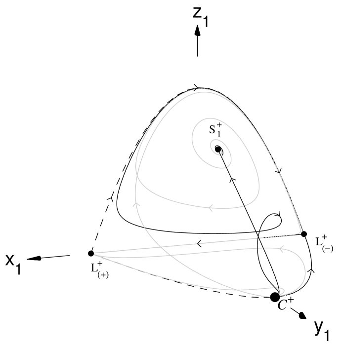
8.2.2 The Case $\Lambda<0$, $\Lambda_{\rm M}>0$

In this case, the negative sign in (8.4) for $y_{2}$ is chosen as is the positive sign for $z_{2}$, and the definition $\xi^{2}=\dot{\varphi}^{2}-2\Lambda$ is chosen. The generalized Friedmann constraint equation is now written to read

$$0\leq x_{2}^{2}+z_{2}\leq 1,$$ (8.8)

and $u_{2}^{2}+y_{2}=1$. Thus $y_{2}$ is considered the extraneous variable and so three-dimensional system consists of the variables $0\leq\{x_{2}^{2},u_{2}^{2},z_{2}\}\leq 1$:

$$\frac{dx_{2}}{dT} = \sqrt{3}\left(1-x_{2}^{2}-\frac{3}{2}z_{2}\right)+x_{2}u_{2}\left(1-x_{2}^{2}-\frac{1}{2}z_{2}\right),$$ (8.9a)

$$\frac{du_{2}}{dT} = (1-u_{2}^{2})\left(x_{2}^{2}+\frac{1}{2}z_{2}\right)>0,$$ (8.9b)

$$\frac{dz_{2}}{dT} = z_{2}\left[u_{2}\left(1-2x_{2}^{2}-z_{2}\right)+\sqrt{3}x_{2}\right].$$ (8.9c)

The invariant sets $x_{2}^{2}+z_{2}=1$, $z_{2}=0$, $u_{2}^{2}=1$ define the boundary of the phase space. Note that $u_{2}$ is monotonically increasing. The equilibrium sets and their corresponding eigenvalues (denoted by $\lambda$) are

$$S^{\pm}_{1}: \left(x_{2},u_{2},z_{2}\right)=\left(\frac{\mp 1}{\sqrt{27}},\pm 1,\frac{16}{27}\right);$$ (8.10a)

$$\left(\lambda_{1},\lambda_{2},\lambda_{3}\right)=\frac{1}{3}\left(\pm 1+i\sqrt{\frac{77}{27}},\pm 1-i\sqrt{\frac{77}{27}},\mp 2\right),$$

$$L^{+}_{(\pm)}: \left(x_{2},u_{2},z_{2}\right)=\left(\pm 1,1,0\right);$$ (8.10b)

$$\left(\lambda_{1},\lambda_{2},\lambda_{3}\right)=\left(\pm\left[\sqrt{3}\mp 1\right],\mp 2\left[\sqrt{3}\pm 1\right],-2\right),$$

$$L^{-}_{(\pm)}: \left(x_{2},u_{2},z_{2}\right)=\left(\pm 1,-1,0\right);$$ (8.10c)

$$\left(\lambda_{1},\lambda_{2},\lambda_{3}\right)=\left(\pm\left[\sqrt{3}\pm 1\right],\mp 2\left[\sqrt{3}\mp 1\right],2\right).$$

Similar to the points $L^{+}_{(\pm)}$, which represent the two $\dot{\varphi}>0$ dilaton–vacuum solutions (6.7) for $h_{0}=\frac{\pm 1}{\sqrt{3}}$, the two points $L^{-}_{(\pm)}$ represent the two $\dot{\varphi}<0$ dilaton–vacuum solutions (6.7) for $h_{0}=\frac{\pm 1}{\sqrt{3}}$.

In this phase space, there are no repelling/attracting equilibrium points, but $u_{2}$ is monotonically increasing. The early-time and late-time behaviour is similar to the late-time behaviour discussed in the previous subsection. Into the past, there are heteroclinic orbits which spend considerable time near the saddle points $L^{-}_{(-)}$ and $L^{-}_{(+)}$, in between which they shadow the lines $u_{2}=-1$, $x_{2}^{2}+z_{2}=1$ and $u_{2}=-1$, $z_{2}=0$. The late-time behaviour is again for trajectories to follow heteroclinic orbits which spend time near the saddles $L^{+}_{(-)}$ and $L^{+}_{(+)}$, in between which they shadow the lines $u_{2}=+1$, $x_{2}^{2}+z_{2}=1$ and $u_{2}=+1$, $z_{2}=0$. In the invariant set $u_{2}=-1$ (which is the past-attracting invariant set) these orbits spiral towards the expanding solution $S^{-}_{1}$, which represents the $t>0$ solution of (7.1). In the future-attracting invariant set, $u_{2}=+1$, orbits spiral away from the contracting solution $S^{+}_{1}$, which represents the $t<0$ solution of (7.1). Figure 8.2 depicts typical trajectories in this phase space.

Figure 8.2: Phase diagram of the system (8.9a) ($\Lambda<0$, $\Lambda_{\rm M}>0$). See also caption to figure 6.1 on page 6.1.

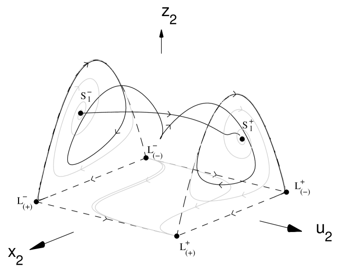
8.2.3 The Case $\Lambda>0$, $\Lambda_{\rm M}<0$

For this case, $\xi^{2}=\dot{\varphi}^{2}-L$ is chosen and from (8.4) the positive sign for $y_{3}$ and the negative sign for $z_{3}$ are chosen in order for these variables to be positive definite. The generalized Friedmann constraint equation can be rewritten as

$$0\leq x_{3}^{2}+y_{3}\leq 1,\qquad u_{3}^{2}+z_{3}=1,$$ (8.11)

and $z_{3}$ may be eliminated to yield the four-dimensional system of ODEs for $0\leq\{x_{3}^{2},y_{3},u_{3}^{2}\}\leq 1$:

$$\frac{dx_{3}}{dT} = x_{3}u_{3}\left(1-x_{3}^{2}\right)+\sqrt{3}\left[\frac{1}{2}\left(1-x_{3}^{2}\right)\left(3-u_{3}^{2}\right)-y_{3}\right],$$ (8.12a)

$$\frac{dy_{3}}{dT} = -x_{3}y_{3}\left[\sqrt{3}\left(1-u_{3}^{2}\right)+2x_{3}u_{3}\right],$$ (8.12b)

$$\frac{du_{3}}{dT} = -\frac{1}{2}\left(1-u_{3}^{2}\right)\left(1-2x_{3}^{2}+\sqrt{3}x_{3}u_{3}\right).$$ (8.12c)

The invariant sets $x_{3}^{2}+y_{3}=1$, $u_{3}^{2}=1$, $y_{3}=0$ define the boundary of the phase space. The equilibrium sets and their corresponding eigenvalues (denoted by $\lambda$) are

$$R: \left(x_{3},y_{3},u_{3}\right)=\left(1,0,\frac{1}{\sqrt{3}}\right);$$ (8.13a)

$$\left(\lambda_{1},\lambda_{2},\lambda_{3}\right)=-\frac{1}{\sqrt{3}}\left(1,4,10\right),$$

$$A: \left(x_{3},y_{3},u_{3}\right)=\left(-1,0,-\frac{1}{\sqrt{3}}\right);$$ (8.13b)

$$\left(\lambda_{1},\lambda_{2},\lambda_{3}\right)=\frac{1}{\sqrt{3}}\left(1,4,10\right),$$

$$C^{\pm}: \left(x_{1},y_{1},u_{1}\right)=\left(0,1,\pm 1\right);$$ (8.13c)

$$\left(\lambda_{1},\lambda_{2},\lambda_{3}\right)=\left(0,\pm 1,\pm 1\right),$$

$$L^{+}_{(\pm)}: \left(x_{3},y_{3},u_{3}\right)=\left(\pm 1,0,1\right);$$ (8.13d)

$$\left(\lambda_{1},\lambda_{2},\lambda_{3}\right)=\left(\pm\left[\sqrt{3}\mp 1\right],\mp 2\left[\sqrt{3}\pm 1\right],-2\right),$$

$$L^{-}_{(\pm)}: \left(x_{3},y_{3},u_{3}\right)=\left(\pm 1,0,-1\right);$$ (8.13e)

$$\left(\lambda_{1},\lambda_{2},\lambda_{3}\right)=\left(\pm\left[\sqrt{3}\pm 1\right],\mp 2\left[\sqrt{3}\mp 1\right],2\right),$$

$$J^{\pm}: \left(x_{3},y_{3},u_{3}\right)=\left(\frac{\pm 1}{\sqrt{5}},\frac{4}{5},\mp\sqrt{\frac{3}{5}}\right);$$ (8.13f)

$$\left(\lambda_{1},\lambda_{2},\lambda_{3}\right)=\frac{1}{\sqrt{5}}\left(\frac{\sqrt{19}\mp\sqrt{3}}{2\sqrt{5}},\frac{-\sqrt{19}\mp\sqrt{3}}{2\sqrt{5}},\mp 2\sqrt{\frac{3}{5}}\right).$$

Again, the points $C^{\pm}$ are non-hyperbolic, but it can be shown that $C^{+}$ is a source whilst $C^{-}$ is a sink. The zero eigenvalue corresponds to a eigenvector lying within the invariant set $u_{3}=+1$. It is easily seen from (8.12b) that $y_{3}$ is monotonically decreasing within this invariant set, moving away from $C^{+}$. Similarly for this invariant set, equation (8.12a) is negative for $y_{3}>(1-x_{3}^{2})(x_{3}+\sqrt{3})/\sqrt{3}$, and (8.12a) is positive for $y_{1}<(1-x_{3}^{2})(x_{3}+\sqrt{3})/\sqrt{3}$. The line $y_{1}=(1-x_{3}^{2})(x_{3}+\sqrt{3})/\sqrt{3}$ includes the equilibrium point $C^{+}$. Hence, the $x_{1}$-component of the trajectories move away from this line. Since $y_{3}$ is monotonically decreasing, then trajectories move away from $C^{+}$ in this invariant set, making $C^{+}$ a source. For points very close to $x_{3}=0$ equation (8.12c) is negative in the full three-dimensional set. Hence, $C^{+}$ is a source for the three-dimensional system. Similarly, $C^{-}$ is a sink. These two points represent the linear dilaton–vacuum solutions (6.12). The point $R$, which acts as a source, represents the “$+$” solution of equation (7.8), and the point $A$, which acts as a sink, is the “$-$” solution of equation (7.8). The four points $L^{\pm}_{(\pm)}$ are saddle points, as are the two equilibrium points $J^{\pm}$, representing the de Sitter-like solutions (8.3).

Hence, solutions asymptote into the past towards either $C^{+}$ or $R$ and asymptote into the future towards either $C^{-}$ or $A$. Figure 8.3 depicts typical trajectories in this phase space.

Figure 8.3: Phase diagram of the system (8.12a) ($\Lambda>0$, $\Lambda_{\rm M}<0$). See also caption to figure 6.1 on page 6.1.

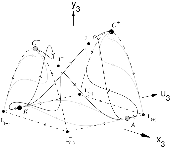
8.2.4 The Case $\Lambda<0$, $\Lambda_{\rm M}<0$

The negative signs for both $y_{4}$ and $z_{4}$ from (8.4) are chosen in this case, as well as the definition $\xi^{2}=\dot{\varphi}^{2}-2\Lambda-L$. The generalized Friedmann constraint equation is now written to read

$$0\leq x_{4}^{2}\leq 1,\qquad u_{4}^{2}+z_{4}+y_{4}=1,$$ (8.14)

Again, $z_{4}$ is considered to be the extraneous variable, resulting in the three-dimensional system consisting of the variables $0\leq\{x_{4}^{2},y_{4},u_{4}^{2}\}\leq 1$:

$$\frac{dx_{4}}{dT} = \frac{1}{2}\left(1-x_{4}^{2}\right)\left[2x_{4}u_{4}+\sqrt{3}\left(3-y_{4}-u_{4}^{2}\right)\right]>0,$$ (8.15a)

$$\frac{dy_{4}}{dT} = -x_{4}y_{4}\left[2x_{4}u_{4}+\sqrt{3}\left(1-y_{4}-u_{4}^{2}\right)\right],$$ (8.15b)

$$\frac{du_{4}}{dT} = -\frac{1}{2}\left(1-u_{4}^{2}\right)\left(1-2x_{4}^{2}+\sqrt{3}x_{4}u_{4}\right)+y_{4}x_{4}^{2}.$$ (8.15c)

The invariant sets $x_{4}^{2}=1$, $u_{4}^{2}+y_{4}=1$, $y_{4}=0$ define the boundary of the phase space. The variable $x_{4}$ is monotonically increasing. The equilibrium sets and their corresponding eigenvalues (denoted by $\lambda$) are

$$R: \left(x_{4},y_{4},u_{4}\right)=\left(1,0,\frac{1}{\sqrt{3}}\right);$$ (8.16a)

$$\left(\lambda_{1},\lambda_{2},\lambda_{3}\right)=-\frac{1}{\sqrt{3}}\left(1,4,10\right),$$

$$A: \left(x_{4},y_{4},u_{4}\right)=\left(-1,0,-\frac{1}{\sqrt{3}}\right);$$ (8.16b)

$$\left(\lambda_{1},\lambda_{2},\lambda_{3}\right)=\frac{1}{\sqrt{3}}\left(1,4,10\right),$$

$$L^{+}_{(\pm)}: \left(x_{4},y_{4},u_{4}\right)=\left(\pm 1,0,1\right);$$ (8.16c)

$$\left(\lambda_{1},\lambda_{2},\lambda_{3}\right)=\left(\pm\left[\sqrt{3}\mp 1\right],\mp 2\left[\sqrt{3}\pm 1\right],\mp 2\right),$$

$$L^{-}_{(\pm)}: \left(x_{4},y_{4},u_{4}\right)=\left(\pm 1,0,-1\right);$$ (8.16d)

$$\left(\lambda_{1},\lambda_{2},\lambda_{3}\right)=\left(\pm\left[\sqrt{3}\pm 1\right],\mp 2\left[\sqrt{3}\mp 1\right],\pm 2\right).$$

The global source for this system is the point $R$, which corresponds to the “$+$” solution of (7.8), and the global sink is the point $A$, which corresponds to the “$-$” solution of (7.8). Figure 8.4 depicts typical trajectories in this phase space.

Figure 8.4: Phase diagram of the system (8.15a) ($\Lambda<0$, $\Lambda_{\rm M}<0$). See also caption to figure 6.1 on page 6.1.

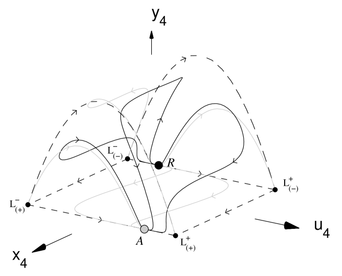
8.3 Summary of Analysis in the Jordan Frame

This discussion begins with two tables; Table 8.1 lists which terms are the dominant variables for each equilibrium set as well as the deceleration parameter, $q$, for the corresponding model and Table 8.2 lists the attracting behaviour of the equilibrium sets occur as early-, intermediate- and late-time attractors.

Set	Dominant Variables							$q$	H
$L^{+}_{(\pm)}$ ($t<0$)	$\alpha$	$\hat{\Phi}$						$1\mp\sqrt{3}$	$\pm\frac{1}{\sqrt{3}}(-t)^{-1}$
$L^{-}_{(\pm)}$ ($t>0$)	$\alpha$	$\hat{\Phi}$						$\pm\sqrt{3}-1$	$\pm\frac{1}{\sqrt{3}}t^{-1}$
$S_{1}^{+}$ ($t<0$)	$\alpha$	$\hat{\Phi}$	$\dot{\sigma}$			$\Lambda_{\rm M}>0$		$2$	$\frac{1}{3}t^{-1}$
$S_{1}^{-}$ ($t>0$)	$\alpha$	$\hat{\Phi}$	$\dot{\sigma}$			$\Lambda_{\rm M}>0$		$2$	$\frac{1}{3}t^{-1}$
$A$ ($t<0$)	$\alpha$	$\hat{\Phi}$				$\Lambda_{\rm M}<0$		$-3$	$-\frac{1}{2}t^{-1}$
$R$ ($t>0$)	$\alpha$	$\hat{\Phi}$				$\Lambda_{\rm M}<0$		$-3$	$-\frac{1}{2}t^{-1}$
$J^{-}$	$\alpha$				$\Lambda>0$	$\Lambda_{\rm M}<0$		$-1$	$-\sqrt{\frac{1}{6}\Lambda}$
$J^{+}$	$\alpha$				$\Lambda>0$	$\Lambda_{\rm M}<0$		$-1$	$\sqrt{\frac{1}{6}\Lambda}$
$C^{\pm}$		$\hat{\Phi}$			$\Lambda>0$			$0$	$0$
$L_{1}$		$\hat{\Phi}$	$\dot{\sigma}$	$k\geq 0$	$\Lambda>0$			$0$	$0$
$N$ ($t<0$)	$\alpha$	$\hat{\Phi}$		$k<0$		$\Lambda_{\rm M}>0$		$0$	$t^{-1}$

Table 8.1: The dominant variables for each equilibrium set as well as the equilibrium set’s deceleration parameter, $q$, and Hubble parameter $H$. Inflation occurs when $q<0$ and $H>0$, whereas “deflation” occurs for $q>0$ and $H<0$. Note that for $L^{+}_{(\pm)}$ and $L^{-}_{(\pm)}$, $h_{0}=\frac{\pm 1}{\sqrt{3}}$

Note that the only inflationary models are those represented by $L^{+}_{(-)}$, $A$ and $J^{+}$. The saddle point $S^{+}_{1}$ represents a deflating model ($q>0$, $H<0$).

Case		Early	Intermediate	Late
$\Lambda>0$	$\Lambda_{\rm M}>0$	$C^{+}$	$S_{1}^{+}$, $L^{+}_{(\pm)}$	$-$
$\Lambda<0$	$\Lambda_{\rm M}>0$	$-$	$S^{\pm}_{1}$, $L^{\pm}_{(\pm)}$	$-$
$\Lambda>0$	$\Lambda_{\rm M}<0$	$C^{+}$, $R$	$L^{\pm}_{(\pm)}$, $J^{\pm}$	$C^{-}$, $A$
$\Lambda<0$	$\Lambda_{\rm M}<0$	$R$	$L^{\pm}_{(\pm)}$	$A$

Table 8.2: Summary of the early-time, intermediate, and late-time attractors for the various models examined. Note that $\dot{\alpha}$, $\hat{\Phi}$ and $\dot{\sigma}$ are present in every model.

Monotonic functions have been established in all cases which precludes the existence of recurrent or periodic orbits, thereby allowing the early-time and late-time behaviour conclusions to be made based upon the equilibrium sets of the system.

For $\Lambda>0$ and $\Lambda_{\rm M}>0$, solutions generically asymptote in the future towards the $y_{1}=0$ invariant set which includes the heteroclinic orbit seen previously in the $\Lambda=0$, $\Lambda_{\rm M}>0$ model, although the solution represented by $S^{+}_{1}$ is no longer a source to the system, but rather a saddle. Since there are no sinks, orbits evolve to the future toward $y_{1}=0$ (with $y_{1}$ monotonically decreasing) and shadow the heteroclinic orbit mimicking the the behaviour of figure 6.1, whereby solutions alternate between the dilaton–vacuum solutions corresponding to the saddle points $L^{+}_{(-)}$ and $L^{+}_{(+)}$, where the central charge deficit and $\Lambda_{\rm M}$ are dynamically negligible. Solutions generically asymptote in the past towards the static, linear dilaton–vacuum solution corresponding to the global source $C^{+}$, at which $\Lambda_{\rm M}$ is dynamically negligible.

In the case where $\Lambda<0$ and $\Lambda_{\rm M}>0$, there are no sinks nor sources in the full 3-dimensional phase-space! The variable $u_{2}$ (and hence $\dot{\varphi}$) is monotonically increasing, evolving from $u_{2}=-1$ to $u_{2}=+1$. Solutions generically asymptote in both the past and future towards invariant sets which include an heteroclinic orbit; i.e., they have a similar asymptotic behaviour at both early and late times to the late-time behaviour of the previous cases of $\Lambda_{\rm M}>0$, alternating between the dilaton–vacuum solutions corresponding to the saddle points $L^{-}_{(\pm)}$ in the past and the dilaton–vacuum solutions corresponding to the saddle points ($L^{-}_{(-)}$ represents an inflationary model) $L^{+}_{(\pm)}$ to the future. Note that $\Lambda_{\rm M}$ is dynamically significant at both early and late times.

In the case where $\Lambda>0$ and $\Lambda_{\rm M}<0$, solutions asymptote into the past towards either the $\dot{\varphi}>0$ linear dilaton–vacuum solution (6.12) or the contracting, static-moduli solution (7.8). Similarly, solutions asymptote into the future either the $\dot{\varphi}<0$ linear dilaton–vacuum solution (6.12) or the expanding, static-moduli solution (7.8). Hence both $\Lambda$ and $\Lambda_{\rm M}$ can be dynamically significant at both early and late times.

When $\Lambda<0$ and $\Lambda_{\rm M}<0$ solutions only asymptote towards the the contracting/expanding, static-moduli solution to the past/future. Because $x_{4}$ monotonically increases, it would seem that a bouncing cosmology from a contracting phase to an expanding phases is typical within this model. The central charge deficit is only dynamically significant at intermediate times, whereas $\Lambda_{\rm M}$ is dynamically significant at both early and late times.

In general, there are only a few cases where $\Lambda$ and $\Lambda_{\rm M}$ are both dynamically significant at early times or at late times. In particular, $\Lambda$ is only dynamically significant at early/late times when $\Lambda>0$, whereas $\Lambda_{\rm M}$ is typically dynamically significant for both early and late times. Because most phase diagrams exhibited some sort of transition from $\dot{\alpha}<0$ to $\dot{\alpha}>0$ (or vice versa) it has been found that bounce cosmologies are fairly typical within these class of models.

8.4 Exact Solutions in the Einstein Frame

The de Sitter solutions transform to

$$J^{\mp}: a^{*}=a^{*}_{0}e^{\pm\sqrt{\frac{1}{6}\Lambda}t_{*}}\qquad\Rightarrow\qquad\!\,^{{}^{\mbox{\rm\tiny(sf)}}}\!H=\pm\sqrt{\frac{1}{6}\Lambda}\qquad\Rightarrow\qquad\!\,^{{}^{\mbox{\rm\tiny(sf)}}}\!q=-1,$$ (8.17)

$$\phi=\phi_{0},$$

$$\Lambda_{\rm M}=-\Lambda e^{-\varepsilon\sqrt{2}\phi_{0}},$$

$$\beta=\beta_{0},$$

$$\sigma=\sigma_{0},$$

$$k=0,$$

Note that $J^{+}$ represents the only inflationary model (of the exact solutions) in the Einstein frame. In the analysis for $\Lambda>0$, $\Lambda_{\rm M}<0$ it was shown that both de Sitter solutions arise as saddles and are dynamically important for intermediate times.

All of the other exact solutions have been specified in the Einstein frame in sections 6.6 (page 6.6) and 7.5 (page 7.5).

8.4.1 Mathematical Equivalence to Matter Terms in the Einstein Frame

The exact solutions discussed in this chapter will now be transformed to a theory of general relativity (Einstein frame) containing a matter field and a scalar field with exponential potential; i.e., $V=V_{0}e^{k\phi}$, where either $k^{2}=2$ or $k^{2}=8$. Similar to subsection 6.6.1 (page 6.6.1), there will be interaction terms between the matter and scalar field (see equation (6.47a) on page 6.47a).

Just like in the previous two chapters, there are two scenarios from which to choose:

1. $V=\Lambda e^{\sqrt{2}\varepsilon\phi}$ $(k^{2}=2)$, ${\cal U}=\frac{1}{2}\Lambda_{\rm M}e^{2\sqrt{2}\varepsilon\phi}$
   The interaction term for this case is $\delta=-2\sqrt{2}\varepsilon\dot{\phi}\ p$.

2. $V=\frac{1}{2}\Lambda_{\rm M}e^{2\sqrt{2}\varepsilon\phi}$ $(k^{2}=8)$ ${\cal U}=\Lambda e^{\sqrt{2}\varepsilon\phi}$
   The interaction term for this case is $\delta=-\frac{\sqrt{2}}{2}\varepsilon\dot{\phi}(\mu+3p)$.

For these two scenarios, the matter field is defined by

$$\mu \equiv \frac{1}{4}\dot{\sigma}^{2}e^{2\sqrt{2}\varepsilon\phi}+{\cal U}$$ (8.18a)

$$p \equiv \frac{1}{4}\dot{\sigma}^{2}e^{2\sqrt{2}\varepsilon\phi}-{\cal U}$$ (8.18b)

and do not in general represent barotropic matter with linear equations of state [$p=(\gamma-1)\mu$], although the equations of state are linear at the equilibrium points. Tables 8.3 and 8.4 list $\{\mu,p,\gamma,\mu_{\phi},p_{\phi},\gamma_{\phi},\delta\}$ for each equilibrium set in each of the two scenarios discussed above.

Scenario A:   $V=\Lambda e^{\sqrt{2}\varepsilon\phi}$,   ${\cal U}=\frac{1}{2}\Lambda_{\rm M}e^{2\sqrt{2}\varepsilon\phi}$,   $\delta=-2\sqrt{2}\varepsilon\dot{\phi}\ p$
Set	$\mu$	$p$	$\gamma$	$\mu_{\phi}$	$p_{\phi}$	$\gamma_{\phi}$	$\delta$
$L^{\pm}_{(\pm)}$	$0$	$0$	$-$	$\frac{1}{3}t_{*}^{-2}$	$\mu_{\phi}$	$2$	$0$
$C^{\pm}$	$0$	$0$	$-$	$3t_{*}^{-2}$	$-t_{*}^{-2}$	$\frac{2}{3}$	$0$
$S_{1}^{\pm}$	$\frac{13}{12}t_{*}^{-2}$	$-\frac{1}{4}t_{*}^{-2}$	$\frac{10}{13}$	$\frac{1}{4}t_{*}^{-2}$	$\mu_{\phi}$	$2$	$-\frac{1}{2}t_{*}^{-3}$
$R/A$	$-\frac{1}{4}t_{*}^{-2}$	$-\mu$	$0$	$\frac{1}{4}t_{*}^{-2}$	$\mu_{\phi}$	$2$	$\frac{1}{2}t_{*}^{-3}$
$J^{\pm}$	$-\frac{1}{2}\Lambda$	$-\mu$	$0$	$\Lambda$	$-\mu_{\phi}$	$0$	$0$

Table 8.3: The matter terms ($\mu$, $p$, $\gamma$) as well as $\mu_{\phi}$, $p_{\phi}$, $\gamma_{\phi}$ and $\delta$ for each of the equilibrium sets derived in scenario A.

From section 8.3, the asymptotic behaviour of the models in the Einstein frame is known and comments on which solutions represent asymptotic states in the Einstein frame are equally applicable here.

In scenario A, solutions asymptote to models in which the matter field is either vacuum ($\mu=p=0$) or are in false vacuum state ($\gamma=0$). As was the case in subsection 7.5.1 (7.5.1), the heteroclinic sequences asymptote to solutions in which the matter field oscillates between a false vacuum ($\gamma=0$) and a true vacuum ($\mu=p=0$).

Scenario B:   $V=\frac{1}{2}\Lambda_{\rm M}e^{2\sqrt{2}\varepsilon\phi}$,  ${\cal U}=\Lambda e^{\sqrt{2}\varepsilon\phi}$,   $\delta=-\frac{\sqrt{2}}{2}\varepsilon\dot{\phi}(\mu+3p)$
Set	$\mu$	$p$	$\gamma$	$\mu_{\phi}$	$p_{\phi}$	$\gamma_{\phi}$	$\delta$
$L^{\pm}_{(\pm)}$	$0$	$0$	$-$	$\frac{1}{3}t_{*}^{-2}$	$\mu_{\phi}$	$2$	$0$
$C^{\pm}$	$2t_{*}^{-2}$	$-\mu$	$0$	$t_{*}^{-2}$	$\mu_{\phi}$	$2$	$-4t^{-3}$
$S_{1}^{\pm}$	$\frac{5}{12}t_{*}^{-2}$	$p$	$2$	$\frac{11}{12}t_{*}^{-2}$	$-\frac{5}{12}t_{*}^{-2}$	$\frac{6}{11}$	$\frac{5}{6}t_{*}^{-3}$
$R/A$	$0$	$0$	$-$	$0$	$\frac{1}{2}t_{*}^{-2}$	$-$	$0$
$J^{\pm}$	$\Lambda$	$-\mu$	$0$	$-\frac{1}{2}\Lambda$	$-\mu_{\phi}$	$0$	$0$

Table 8.4: The matter terms ($\mu$, $p$, $\gamma$) as well as $\mu_{\phi}$, $p_{\phi}$, $\gamma_{\phi}$ and $\delta$ for each of the equilibrium sets derived in scenario B.

Similar to scenario A, in scenario B solutions asymptote to models in which the matter field is either absent ($\mu=p=0$) or is a false vacuum ($\gamma=0$), although the equation of state is reversed to that in scenario A for the solutions at the asymptotic equilibrium points. Here, the heteroclinic orbits asymptotically represent solutions in which the matter field becomes negligible in any part of the cycle.

Chapter 9 String Models IV: Ramond–Ramond Term ($\Lambda_{\rm M}=0$)

In this chapter, the field equations (6.5a) are considered when $Q\neq 0$. Of primary interest is how these equations evolve for flat FRW models with neither a central charge deficit nor a $\Lambda_{\rm M}$ term. However, it is straightforward to perform a perturbation analysis to the curvature term and the $\Lambda$ term, allowing a comment to be made about the stability of these models to curvature or $\Lambda$ perturbations. It should be stressed that within the string context, the central charge deficit does not naturally arise in the type IIA supergravity theory where the Ramond–Ramond term arises, but it will be included in section 9.2.4 as a perturbation parameter, and as a source for the exponential potential in the Einstein frame. If $k<0$ and $\Lambda>0$, the variables used lead to a compact five-dimensional phase space and so the global qualitative analysis shall be restricted to this case. Note that all the local results (e.g., stability of equilibrium points) obtained will also be true for the case $k>0$ (as well as $\Lambda>0$).

The chapter is organized as follows. In section 9.1, the field equations (6.5a) and (6.6) are reexamined with $\Lambda_{\rm M}=0$. Section 9.2 proceeds with the analysis of the equations. The chapter ends with a summary section and a section which discusses the corresponding solutions and asymptotic behaviour in the Einstein frame. Again, this chapter is primarily confined to the Jordan frame (except the final section), and so the index “(st)” shall be omitted to save notation (but must be introduced again in the final section when both frames are discussed).

9.1 Governing Equations

For $Q\neq 0$, $\Lambda=\Lambda_{\rm M}=0$, there exists the solution not found in the previous chapters:

$$a = a_{0}\left(\pm\varsigma t\right),$$ (9.1)

$$\hat{\Phi} = \hat{\Phi}_{0}-\frac{4}{5}\ln\left(\pm\varsigma t\right),$$

$$\beta = \beta_{0}+\frac{1}{5}\ln\left(\pm\varsigma t\right),$$

$$\sigma = \sigma_{0},$$

$$k = -\frac{3}{2}Q^{2}e^{\hat{\Phi}_{0}+2\alpha_{0}-6\beta_{0}},$$ (9.2)

where $\varsigma=\frac{5}{2\sqrt{7}}Q\mbox{exp}\left\{\frac{1}{2}(\hat{\Phi}_{0}-6\beta_{0})\right\}$ and $\{a_{0}=e^{\alpha_{0}},\hat{\Phi}_{0},\beta_{0},\sigma_{0}\}$ are constants. The “$-$” solutions correspond to $t<0$ whilst the “$+$” correspond to the $t>0$ solutions. These solutions are represented in the text by the equilibrium points $T$. Since the non-negligible terms are the same as equation (6.7) with the addition of a curvature term, this solution will be referred to as the “curved dilaton–moduli–vacuum” solutions, although it does not reduce to (6.7) when $k=0$.

By introducing a new time variable via

$$\frac{d}{d\eta}={\rm e}^{-\frac{1}{2}(-6\beta+\varphi+3\alpha)}\frac{d}{dt},$$ (9.3)

the field equations (6.5a) may be written

$$\alpha^{\prime\prime} = \frac{1}{2}\alpha^{\prime}\varphi^{\prime}+3\alpha^{\prime}\beta^{\prime}-\frac{9}{2}\left(\alpha^{\prime}\right)^{2}+\left(\varphi^{\prime}\right)^{2}-6\left(\beta^{\prime}\right)^{2}+4k{\rm e}^{-(5\alpha+\varphi-6\beta)}$$ (9.4a)

$$\qquad\qquad-2\Lambda e^{-(3\alpha+\varphi-6\beta)}+\frac{3}{4}Q^{2},$$

$$\varphi^{\prime\prime} = 3\left(\alpha^{\prime}\right)^{2}+6\left(\beta^{\prime}\right)^{2}+\frac{1}{4}Q^{2}-\frac{1}{2}\left(\varphi^{\prime}\right)^{2}+3\beta^{\prime}\varphi^{\prime}-\frac{3}{2}\alpha^{\prime}\varphi^{\prime},$$ (9.4b)

$$\beta^{\prime\prime} = \frac{1}{2}\beta^{\prime}\varphi^{\prime}+3\left(\beta^{\prime}\right)^{2}-\frac{3}{2}\alpha^{\prime}\beta^{\prime}+\frac{1}{4}Q^{2},$$ (9.4c)

and the Friedman constraint may be written

$$\frac{1}{2}\rho e^{-3\alpha-\varphi+6\beta}=\left(\varphi^{\prime}\right)^{2}-3\left(\alpha^{\prime}\right)^{2}-6\left(\beta^{\prime}\right)^{2}+6ke^{-(5\alpha+\varphi-6\beta)}-2\Lambda e^{-(3\alpha+\varphi-6\beta)}-\frac{1}{2}Q^{2}.$$ (9.5)

Furthermore, these equations may be further reduced by defining the variables

$$x=\frac{\sqrt{3}\alpha^{\prime}}{\varphi^{\prime}}\ ,\ y=\frac{\sqrt{6}\beta^{\prime}}{\varphi^{\prime}}\ ,\ z=\frac{\frac{1}{2}Q^{2}}{(\varphi^{\prime})^{2}}\ ,\ u=-\frac{6ke^{-(5\alpha+\varphi-6\beta)}}{(\varphi^{\prime})^{2}}\ ,\ v=\frac{2\Lambda e^{-(3\alpha+\varphi-6\beta)}}{(\varphi^{\prime})^{2}}\ ,$$ (9.6)

and a new reduced time variable, $\tau$,

$$\frac{d}{d\tau}=\left(\varphi^{\prime}\right)^{-1}\frac{d}{d\eta},$$ (9.7)

(where it is assumed that $\varphi^{\prime}>0$) to yield the equations

$$\frac{dx}{d\tau} = \left(1-x^{2}-y^{2}-z\right)(x+\sqrt{3})+\frac{1}{2}z\left(x-\sqrt{3}\right)-\frac{2}{\sqrt{3}}u-\sqrt{3}v,$$ (9.8a)

$$\frac{dy}{d\tau} = \left(1-x^{2}-y^{2}-z\right)y+\frac{1}{2}z\left(y+\sqrt{6}\right),$$ (9.8b)

$$\frac{dz}{d\tau} = z\left[z-1-\sqrt{6}y+\sqrt{3}x+2\left(1-x^{2}-y^{2}-z\right)\right],$$ (9.8c)

$$\frac{du}{d\tau} = -u\left(\frac{2}{\sqrt{3}}x+z+2x^{2}+2y^{2}\right),$$ (9.8d)

$$\frac{dv}{d\tau} = -v(2x^{2}+2y^{2}+z).$$ (9.8e)

The Friedmann equation (9.5) is now written

$$\frac{1}{2}\rho e^{-3\alpha-\varphi+6\beta}=1-x^{2}-y^{2}-z-u-v,$$ (9.9)

so that it is apparent for $\Lambda>0$, $k<0$ that the variables $0\leq\left\{x^{2},y^{2},z,u,v\right\}\leq 1$ are indeed bounded (this is apparent from equation (9.5); the right side is positive definite and therefore $(\varphi^{\prime})^{2}$ must be larger than the other terms if $\Lambda>0$, $k<0$). From equation (9.8e) it is apparent that $v$ is a monotonically decreasing function.

9.2 Analysis

The equilibrium sets to the system (9.8a) and their corresponding eigenvalues are

$$L^{+}: x^{2}+y^{2}=1,z=u=v=0;$$

$$\left(\lambda_{1},\lambda_{2},\lambda_{3},\lambda_{4},\lambda_{5}\right)=$$

$$\left(0,-2[1+\sqrt{3}x],[\sqrt{3}x-\sqrt{6}y-1],-\frac{2}{\sqrt{3}}\left[x+\sqrt{3}\right],-2\right),$$

$$S^{+}: x=-\frac{1}{\sqrt{3}},y=z=0,u=\frac{2}{3},v=0;$$ (9.10b)

$$\left(\lambda_{1},\lambda_{2},\lambda_{3},\lambda_{4},\lambda_{5}\right)=\left(\frac{4}{3},-\frac{2}{3},\frac{2}{3},\frac{2}{3},-\frac{2}{3}\right),$$

$$C^{+}: x=y=z=u=0,v=1;$$ (9.10c)

$$\left(\lambda_{1},\lambda_{2},\lambda_{3},\lambda_{4},\lambda_{5}\right)=\left(1,0,1,1,0\right),$$

$$T: x=-\frac{5\sqrt{3}}{19},y=-\frac{\sqrt{6}}{19},z=\frac{28}{361},u=\frac{252}{361},v=0;$$ (9.10d)

$$\left(\lambda_{1\atop 2},\lambda_{3},\lambda_{4},\lambda_{5}\right)=\left(\frac{1}{19}\left[7\pm i\sqrt{119}\right],\frac{14}{19},\frac{20}{19},-\frac{10}{19}\right).$$

The equilibrium set $L^{+}$ represent the $\dot{\varphi}>0$ dilaton–moduli–vacuum solutions (6.7) and are sinks in this five dimensional set for $x>-\frac{1}{\sqrt{3}}$ and $\sqrt{2}y>x-\frac{1}{\sqrt{3}}$. The one zero eigenvalue results from the fact that $L^{+}$ is a line of equilibrium points. The equilibrium point $S^{+}$ represents the Milne solution (6.9) and is a saddle. The equilibrium point $C^{+}$ is the linear dilaton–vacuum solution and will be shown to be a source in the five-dimensional system in section 9.2.4. Finally, the equilibrium point $T$ represents a new solution, referred to as the “curved dilaton–moduli–vacuum” solution (9.2) due to its similarity to the dilaton–moduli–vacuum solutions, and is a source in the four–dimensional system $\Lambda=0$ but a saddle in the full five–dimensional system.

9.2.1 Two-Dimensional Invariant Set, $z=u=v=0$ ($Q=k=\Lambda=0$)

The equilibrium points $C^{+}$, $S^{+}$ and $T$ do not exist in this invariant set, and therefore the line $L^{+}$ is the only equilibrium set, with eigenvalues $\lambda_{1}$ and $\lambda_{2}$ given in equation (LABEL:Qdmv). The trajectories in this invariant can be completely solved:

$$y=\frac{y_{0}(x+\sqrt{3})}{x_{0}+\sqrt{3}}\ ,$$ (9.11)

where $(x_{0},y_{0})$ is the initial point of the orbit. The function $x$ is a monotonically increasing function in this invariant set. Figure 9.1 depicts this two-dimensional phase plane. The point $P$ in this portrait corresponds to the point on the line in which both eigenvalues are zero. In the three-dimensional ($\{x,y,z\}$) analysis below, it will be shown to be a source and so it is a source here, albeit non-hyperbolic.

Figure 9.1: Phase portrait of the system (9.8a) for $Q=k=\Lambda=0$. Note that $L^{+}$ represents a line of equilibrium points. See also caption to figure 6.1 on page 6.1.

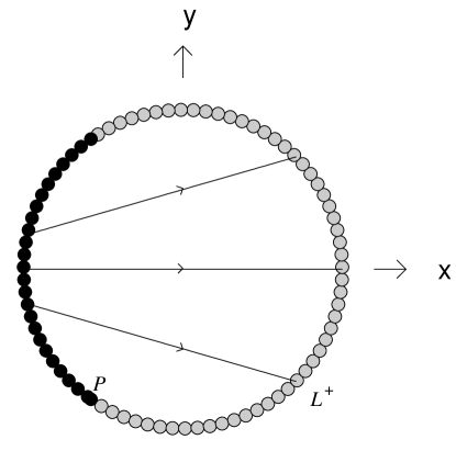
9.2.2 Two-Dimensional Invariant Set, $z=1-x^{2}-y^{2}$, $u=v=0$ ($\rho=k=\Lambda=0$)

Again, the line $L^{+}$ is the only equilibrium set, but this time with eigenvalues $\lambda_{1}$ and $\lambda_{3}$ given in equation (LABEL:Qdmv). The point $P$ on the line $L^{+}$ is again non-hyperbolic, but is a source since it is a source in the three–dimensional system $k=\Lambda=0$. The trajectories in this invariant can also be completely solved:

$$y=-\sqrt{6}+\frac{(y_{0}+\sqrt{6})(x-\sqrt{3})}{x_{0}-\sqrt{3}}\ ,$$ (9.12)

where $(x_{0},y_{0})$ is again the initial point of the orbit. In this invariant set, $x$ is monotonically decreasing while $y$ is monotonically increasing. Figure 9.2 depicts this two-dimensional phase plane.

Figure 9.2: Phase portrait of the system (9.8a) for $\rho=k=\Lambda=0$. Note that $L^{+}$ represents a line of equilibrium points. See also caption to figure 6.1 on page 6.1.

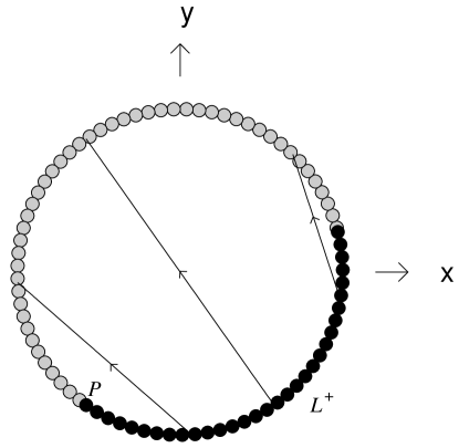
9.2.3 Three-Dimensional Invariant Set, $u=v=0$ ($k=\Lambda=0$)

The equilibrium points $C^{+}$, $S^{+}$ and $T$ do not exist in this invariant set, and therefore the line $L^{+}$ is the only equilibrium set, with eigenvalues $\lambda_{1}$, $\lambda_{2}$ and $\lambda_{3}$ given in equation (LABEL:Qdmv). From these eigenvalues, it has been determined that this line is a sink for $x>-\frac{1}{\sqrt{3}}$ and $\sqrt{2}y>x-\frac{1}{\sqrt{3}}$. The lines $x=-\frac{1}{\sqrt{3}}$ and $\sqrt{2}y=x-\frac{1}{\sqrt{3}}$ intersect on $L^{+}$ at the point $P:(x,y)=\left(-\frac{1}{\sqrt{3}},-\sqrt{\frac{2}{3}}\right)$, at which all three eigenvalues are zero. It shall now be demonstrated that this point is indeed a source to the three-dimensional system.

From equations (9.8a) and (9.8b) for $u=v=0$, is can be shown that

$$\frac{d}{d\tau}\left(x+\sqrt{2}y+\sqrt{3}\right)=\left(x+\sqrt{2}y+\sqrt{3}\right)\left(1-x^{2}-y^{2}-\frac{1}{2}z\right),$$ (9.13)

and hence $x+\sqrt{2}y+\sqrt{3}$ is a monotonically increasing function. Note that the right hand side of (9.13) is zero only at $P$ and positive everywhere else in the phase space. Also, the line tangent to the unit circle at $P$ is $x+\sqrt{2}y=-\sqrt{3}$ and so this monotonic function contains this tangent line as part of its class. Hence, the monotonic function asymptotically approaches the tangent line to the unit circle at point $P$ into the past and hence $P$ is a source for the three-dimensional system. Numerical calculations have verified this point to be a source and the three-dimensional system is depicted in figures 9.3 and 9.4 (the first figure depicts a trajectory which stays near the boundary, whilst the second depicts a more internal trajectory).

Figure 9.3: Phase diagram of the system (9.8a) ($Q\neq 0$). Note that $L^{+}$ represents a line of equilibrium points. Note that the trajectories in figures 9.1 and 9.2 are depicted in this figure along $z=0$ and $z=1-x^{2}-y^{2}$, respectively. See also caption to figure 6.1 on page 6.1.

Figure 9.4: An alternative trajectory within the phase space of the system (9.8a) ($Q\neq 0$). Note that $L^{+}$ represents a line of equilibrium points. See also caption to figure 6.1 on page 6.1.

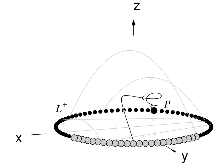
9.2.4 Four- and Five-Dimensional System and Perturbations

The fact that $v$ is monotonically decreasing suggests that $C^{+}$ is a source in the five-dimensional system. Similar to the arguments of subsection 6.4.3 (page 6.4.3), solutions asymptote into the past towards larger values of $v$, the maximum value of which (i.e. $v=1$) coincides with the equilibrium point $C^{+}$ and so it is a source for the system (9.8a). In the invariant set $v=0$, the corresponding eigenvalues to the equilibrium point are $\lambda_{1}$, $\lambda_{2}$, $\lambda_{3}$ and $\lambda_{4}$ found in equations (9.2) and hence the point $T$ represents a source in the four-dimensional set $v=0$. Unfortunately, due to the lack of any monotonic function found in this invariant set, the possibility of recurring orbits cannot be excluded and so it is not possible to say that the attracting set on $L^{+}$ is the sole attracting set of the four-dimensional system.

Although the compactness of the phase space depends on the fact that $k<0$ and $\Lambda>0$, arbitrary signs of $k$ and $\Lambda$ can be assumed and then (9.2) is used in order to determine the local stability of the three-dimensional set $u=v=0$. Specifically, the eigenvalues $\lambda_{4}$ and $\lambda_{5}$ are those related to the eigenvectors extending into the $u$ and $v$ directions, and for $L^{+}$ these eigenvalues are negative. Hence, the line $L^{+}$ is locally attracting trajectories from the $u\neq 0$ and $v\neq 0$ portion of the phase space and so the point $P$ is a only a saddle point in the extended space (for either sign of $k$ and $\Lambda$), whereas the sink portion of $L^{+}$ (i.e. points on $L^{+}$ for $x>-\frac{1}{\sqrt{3}}$ and $\sqrt{2}y>x-\frac{1}{\sqrt{3}}$) is a sink for the extended space (for either sign of $k$ and $\Lambda$). Therefore, the dilaton–moduli–vacuum solutions for $3\dot{\alpha}>-\dot{\varphi}$ and $6\dot{\beta}>3\dot{\alpha}-\dot{\varphi}$ will be attracting solutions for models containing either a curvature term or a central charge deficit.

9.3 Summary of Analysis in the Jordan Frame

This discussion begins with two tables; Table 9.1 lists which terms are the dominant variables for each equilibrium set as well as the deceleration parameter, $q$, for the corresponding model and Table 9.2 lists the attracting behaviour of the equilibrium sets.

Set	Dominant Variables								$q$	H
$L^{+}$ ($t<0$)	$\alpha$	$\hat{\Phi}$	$\dot{\beta}$						$-(1+h_{0})h_{0}^{-1}$	$h_{0}(-t)^{-1}$
$C^{+}$		$\hat{\Phi}$				$\Lambda>0$			$0$	$0$
$S^{+}$	$\alpha$				$k<0$				$0$	$t^{-1}$
$T$	$\alpha$	$\hat{\Phi}$	$\dot{\beta}$		$k<0$			$Q^{2}$	$0$	$t^{-1}$

Table 9.1: The dominant variables for each equilibrium set as well as the equilibrium set’s deceleration parameter, $q$, and Hubble parameter $H$. Inflation occurs when $q<0$ and $H>0$, whereas “deflation” occurs for $q>0$ and $H<0$. Note that the only “anisotropic” solutions are represented by the lines $L^{\pm}$, except when $h_{0}^{2}=\frac{1}{3}$.

Terms Present				Early	Intermediate	Late
$\dot{\beta}$			$Q^{2}$	$L^{+}(P)$	$L^{+}$	$L^{+}$
$\dot{\beta}$	$k<0$		$Q^{2}$	$T$	$S^{+}$, $L^{+}$	$L^{+}$
$\dot{\beta}$	$k<0$	$\Lambda>0$	$Q^{2}$	$C^{+}$	$T$, $S^{+}$, $L^{+}$	$L^{+}$

Table 9.2: Summary of the early-time, intermediate, and late-time attractors for the various models examined. Note that $\dot{\alpha}$, $\hat{\Phi}$ and $\dot{\sigma}$ are present in every model. In the first row, $L^{+}(P)$ refers to the equilibrium point $P$ which lies in the line $L^{+}$.

For the three-dimensional system ($k=\Lambda=0$), a monotonic functions had been established which precludes the existence of recurrent or periodic orbits, thereby allowing the early-time and late-time conclusions of these models to be based upon the equilibrium sets of the system. For the four dimensional case ($\Lambda=0$), a monotonic function could not be determined. Hence, although the equilibrium points in this phase space are still appropriate attracting sets, there may exist periodic orbits in the higher dimensions which may act as asymptotic attracting sets. Therefore, it cannot be asserted, for instance, that the four dimensional phase space asymptotes towards the three dimensional phase space at late times. A monotonically decreasing function exists for the five-dimensional phase space and hence this phase space does asymptote to the four dimensional phase space ($\Lambda=0$) at late times.

In all cases, the $\dot{\varphi}>0$ dilaton–moduli–vacuum solutions (6.7) act as a late-time attractor, and as a source (for one particular point on $L^{+}$ where $h_{0}=-\frac{1}{3}$). The source represents a ten–dimensional isotropic solution ($\dot{\alpha}=\dot{\beta}$). In the presence of a curvature term or a central charge deficit, the late-time behaviour may be the same (again when $k<0$ there was no monotonic function found to ensure that this is true), but evolve from some model in which $k$ or $\Lambda$ is dominant [for example, if $k<0$ and $\Lambda>0$ then possibly either the $\dot{\varphi}>0$ linear dilaton–vacuum solution (6.12) or the curved dilaton–moduli–vacuum solution (9.2)].

As discussed above, the time-reversed dynamics of the above class of models is deduced by interchanging the sources and sinks and reinterpreting expanding solutions in terms of contracting ones, and vice–versa. Thus, the late-time attractor for the time–reversed system is the expanding, isotropic, ten–dimensional cosmology located at point $P$ and all late–time attracting solutions in the post-big bang regime are not inflationary.

9.4 Exact Solutions in the Einstein Frame

For $Q\neq 0$, $\Lambda=\Lambda_{\rm M}=0$, the curved dilaton–moduli–vacuum solution transforms to the Einstein frame to the solution

$$T: a^{*}=a^{*}_{0}\left|t_{*}\right|\qquad\Rightarrow\qquad\!\,^{{}^{\mbox{\rm\tiny(sf)}}}\!H=t_{*}^{-1}\qquad\Rightarrow\qquad\!\,^{{}^{\mbox{\rm\tiny(sf)}}}\!q=0,$$ (9.15)

$$e^{\varepsilon\sqrt{2}\phi}=e^{\varepsilon\sqrt{2}\phi}\left[{\cal A}^{4}\left|\varsigma t_{*}\right|^{\frac{4}{7}}\right]^{-1},$$

$$e^{\beta}=e^{\beta_{0}}\left[{\cal A}\left|\varsigma t_{*}\right|^{\frac{1}{7}}\right],$$

$$\sigma=\sigma_{0},$$

$$k=-\frac{6}{7}a^{*2}_{0},$$

where ${\cal A}=\left[\frac{7}{5}\exp\{\varepsilon\phi_{0}/\sqrt{2}\}\right]^{\frac{1}{7}}$, $a_{0}^{*}=\frac{7}{5}\varsigma a_{0}$ and $\varsigma=\frac{5}{2\sqrt{7}}Q\mbox{exp}\left\{\frac{1}{2}(\hat{\Phi}_{0}-6\beta_{0})\right\}$. The analysis in the Jordan frame shows that this solution arises only as an early-time attractor in the presence of negative curvature, otherwise it is a saddle in a higher-dimensional analysis (including a central charge deficit) or does not exist at all when no curvature is present.

In addition to this solution, this chapter also has as equilibrium sets which represent solutions found in earlier chapters; the solutions in the Einstein frame for these equilibrium points have also been given previously: the linear–dilaton–vacuum solution (equation (6.43) on page 6.43), the Milne solutions (equation (6.44) on page 6.44), and the linear dilaton–vacuum solution (equation (6.45) on page 6.45).

There are no inflationary models in the Einstein frame.

9.4.1 Mathematical Equivalence to Matter Terms

When considering the mathematical equivalence to matter fields in the Einstein frame, the case $Q\neq 0$ differs from the previous cases. In particular, the presence of the $Q$ term does not allow for an equivalence to occur between certain Bianchi models with or without a modulus term and curved FRW models with a modulus field. Therefore, the $\beta$ term is explicitly the modulus field and not a combination of the modulus field with shear terms (as described in equation (6.3) on page 6.3). However, in this case, matter fields can be constructed in the Einstein frame from both the modulus field and the axion field, leading to the conservation equations

$$\dot{\phi}\left(\ddot{\phi}+3\!\,^{{}^{\mbox{\rm\tiny(sf)}}}\!H\dot{\phi}+\frac{dV}{d\phi}\right) = -\delta=\sqrt{2}\varepsilon\dot{\phi}\left[\left(\mu_{2}-\mu_{1}\right)+\left(p_{2}+p_{1}\right)\right],$$ (9.16a)

$$\dot{\mu}_{1}+3\!\,^{{}^{\mbox{\rm\tiny(sf)}}}\!H\left(\mu_{1}+p_{1}\right) = 0$$ (9.16b)

$$\dot{\mu}_{2}+3\!\,^{{}^{\mbox{\rm\tiny(sf)}}}\!H\left(\mu_{2}+p_{2}\right) = \delta=-\sqrt{2}\varepsilon\dot{\phi}\left[\left(\mu_{2}-\mu_{1}\right)+\left(p_{2}+p_{1}\right)\right],$$ (9.16c)

where

$$\mu_{1} \equiv 3\dot{\beta}_{m}^{2}+{\cal U},$$ (9.17a)

$$p_{1} \equiv 3\dot{\beta}_{m}^{2}-{\cal U},$$ (9.17b)

$$\mu_{2} = p_{2}=\frac{1}{4}\dot{\sigma}^{2}e^{2\sqrt{2}\varepsilon\phi}\qquad(\gamma_{2}=2),$$ (9.17c)

and

$${\cal U}=\frac{1}{4}Q^{2}e^{-6\beta_{m}+2\sqrt{2}\varepsilon\phi}.$$ (9.18)

Again, the definition

$$\mu_{\phi} = \frac{1}{2}\dot{\phi}^{2}+V,$$ (9.19a)

$$p_{\phi} = \frac{1}{2}\dot{\phi}^{2}-V,$$ (9.19b)

where

$$V=\Lambda e^{\sqrt{2}\varepsilon\phi}\qquad(k^{2}=2),$$ (9.20)

allows a comparison between $\gamma_{\phi}\equiv(\mu_{\phi}+p_{\phi})/\mu_{\phi}$ and the $\gamma$ of each matter field.

Note that the first matter field ($\mu_{1}$, $p_{1}$) will not represent barotropic matter with a linear equation of state [$p=(\gamma-1)\mu$] in general, although they are at the equilibrium sets. Table 9.3 lists $\{\mu_{1},p_{1},\gamma_{1},\mu_{\phi},p_{\phi},\gamma_{\phi},\mu_{2},\delta\}$ for each equilibrium set.

$V=\Lambda e^{\sqrt{2}\varepsilon\phi}$,   ${\cal U}=\frac{1}{4}Q^{2}e^{-6\beta_{m}+2\sqrt{2}\varepsilon\phi}$,   $\delta=-\sqrt{2}\varepsilon\dot{\phi}\left[\left(\mu_{2}-\mu_{1}\right)+\left(p_{2}+p_{1}\right)\right]$
Set	$\mu_{1}$	$p_{1}$	$\gamma_{1}$	$\mu_{\phi}$	$p_{\phi}$	$\gamma_{\phi}$	$\mu_{2}=p_{2}$	$\delta$
$L^{+}$	$\frac{2(1-3h_{0}^{2})}{9(1+h_{0})^{2}}t_{*}^{-2}$	$\mu_{1}$	$2$	$\frac{(3h_{0}+1)^{2}}{9(1+h_{0})^{2}}t_{*}^{-2}$	$\mu_{\phi}$	$2$	0	$0$
$L^{+}(P)$	$t_{*}^{-2}$	$\mu_{1}$	$2$	$0$	$0$	$-$	0	$0$
$S^{+}$	$0$	$0$	$-$	$0$	$0$	$-$	$0$	$0$
$C^{+}$	$0$	$0$	$-$	$3t_{*}^{-2}$	$-t_{*}^{-2}$	$\frac{2}{3}$	$0$	$0$
$T$	$\frac{10}{49}t_{*}^{-2}$	$-\frac{4}{49}t_{*}^{-2}$	$\frac{3}{5}$	$\frac{4}{49}t_{*}^{-2}$	$\mu_{\phi}$	$2$	$0$	$-\frac{8}{49}t_{*}^{-3}$

Table 9.3: The matter terms ($\mu_{1}$, $p_{1}$, $\gamma_{1}$, $\mu_{2}$) as well as $\mu_{\phi}$, $p_{\phi}$, $\gamma_{\phi}$ and $\delta$ for each of the equilibrium sets. Note that $p_{2}=\mu_{2}$ and hence $\gamma_{2}=2$ for all sets.

As is evident from table 9.3, the second fluid ($\mu_{2}$) approaches a vacuum solution asymptotically (either to the future or the past) and so arises only at intermediate times in which case it is always a stiff fluid. A late-time attractor is the set $L^{+}$ (this is the only late-time attractor when $k=\Lambda=0$). Hence, to the future the first fluid asymptotes towards a stiff equation of state, as does the scalar field contribution. This is the only example in which a matter scaling solution arises from the exact solutions of the string theory. For $P$, which represents an early-time attracting solution in the three-dimensional set, the only energy contribution is from the first fluid. For the past attractor represented by $C^{+}$ (five–dimensional phase space), all matter fields asymptote to a vacuum solution, whereas for the past attractor represented by $T$ (four-dimensional phase space) the first fluid asymptotes towards a model of negative pressure ($\gamma_{1}=\frac{3}{5}$). In the three-dimensional set, the point $P$ (belonging to the set $L^{+}$) is an early-time attractor, and the corresponding matter fields are all vacuum.

Chapter 10 Apodeixis

10.1 Summary

The goal of this thesis was to ascertain the asymptotic properties of cosmological models containing a scalar field, both in the Einstein frame (general relativity minimally coupled to a scalar field) and the Jordan frame (Brans-Dicke theory, scalar-tensor theory and string theory). A formal mathematical equivalence between the two frames was first discussed, explicitly deriving exact solutions in the Brans-Dicke theory from asymptotically stable solutions obtained from a model containing a scalar field with an exponential potential in the Einstein frame. This equivalence was utilized in subsequent chapters to comment on the asymptotic properties of models in both frames. Furthermore, it naturally provides a form for an interaction term studied in the Einstein frame for scalar field models with an exponential potential. In general, the isotropization of the models in the two frames are identical; should a model isotropize in one frame, it will do so in the other. However, inflation is frame dependent and through these mathematical transformations the asymptotic inflationary behaviour in the other frame can be calculated.

In the Einstein frame, scalar fields with an exponential potential (and matter terms) were considered in several contexts. In all cases, the field equations could be written in terms of first order, non-linear, autonomous, ordinary, differential equations and the variables chosen led to a compact phase space; hence, a complete qualitative analysis could be performed. First, the flat FRW matter scaling solutions were subjected to curvature and shear perturbations to examine their stability. Subsequently, a more detailed analysis was performed which examined the asymptotic properties of the spatially-homogeneous Bianchi class B models containing a scalar field with an exponential potential and matter. Monotonic functions were found in many instances, in which cases the global asymptotic results could be fully determined. When monotonic functions could not be found, plausible conjectures were presented about the asymptotic properties. Finally, within the context of flat FRW models, interaction terms were introduced in order to determine if they had a significant effect on the late-time dynamics, particularly with regards to inflation.

The remainder of the thesis was devoted to certain string cosmologies, within the context of both flat FRW models and a class of spatially-homogeneous Bianchi models. Although these models are of great physical interest in their own right, it was shown that they are also related to general relativity containing a scalar field with an exponential potential and matter with a non-linear equation of state, thereby complimenting analyses in previous chapters. In these chapters the qualitative effects of the physical fields arising from string theory, as well as the qualitative effects of curvature and shear, were studied. In each case, a choice of variables leading to a compact phase space was established, thereby allowing a complete analysis. In all of the Bianchi models studied monotonic functions were found allowing global results to be obtained. For the flat FRW models, monotonic functions were found in most cases, and plausible conjectures were made for those cases in which a monotonic function could not be found.

10.2 Conclusions

For the Bianchi class B models containing a scalar field with an exponential potential and matter (and without an interaction term), solutions generically asymptote into the past towards anisotropic models in which matter is negligible and the scalar field is massless ($V=0$); these solutions are a generalization of Jacob’s anisotropic Bianchi I solutions to include scalar fields (represented by the line ${\cal K}$ on page 4.2.2). Towards the future, all models for $k^{2}<2$ asymptote towards an inflationary, isotropic scalar field model in which matter is negligible. Since the Bianchi types VI_h and VII_h are both a one parameter family of models they represent an open class of models to which the other Bianchi types are of zero measure; hence generic behaviour to these two types represent generic behaviour for all Bianchi models. For $k^{2}>2$, Bianchi type VI_h models asymptote to either anisotropic solutions in which matter is negligible (one asymptotic solution is represented by the point $P_{\cal S}^{\pm}(VI_{h})$ on page 4.2.1 and the other by the line ${\cal L}_{l}(VI_{h})$ on page 4.2.2) or to the anisotropic matter scaling solution (represented by the point ${\cal A}_{\cal S}(VI_{h})$ on page 4.2.3). However, this class of models does not admit an isotropic subgroup and isotropization was not expected. For $k^{2}>2$, Bianchi type VII_h models generically asymptote towards a curved, isotropic model in which the matter terms are negligible (either represented by point $P_{\cal S}(V)$ on page 4.2.1 or by the point P${}^{\pm}_{\cal S}(VII_{h})$ on page 4.2.1). Therefore, there exists an open set in the Bianchi class B models which do isotropize to the future and which do not inflate asymptotically. Furthermore, the flat FRW matter scaling solutions are not stable attracting solutions, which was proven both in the perturbation analysis (chapter 3) and in the Bianchi class B analysis (chapter 4). In these models, curvature can play a dynamic rôle at late times (note that the none of Bianchi class B models studied have positive spatially curvature).

It was shown that the presence of an interaction term can considerably change the dynamics the models. In particular, it was shown that when forms for the interaction term discussed in this thesis are used then the flat FRW matter scaling solutions ($\gamma_{\phi}=\gamma$) cannot be represented by an equilibrium point and thus cannot be an asymptotic solution in the models considered here. However, the examples in this thesis have shown that analogous solutions arise, in which both the scalar field and matter terms are non-negligible, but with $\gamma_{\phi}\neq\gamma$. Furthermore, it has been shown to be possible that the power-law inflationary model need not be a late-time attracting solution for $k^{2}<2$; hence, it is possible to have an inflationary model without driving the matter content to zero at late times. The examples given have shown that the stable solutions (which are inflationary) for the same parameter value are spiral nodes representing an oscillating scalar field.

In the string models examined, there are no late-time attracting solutions which inflate in the post-big bang regime. Furthermore, the curvature terms are generically dominant only at intermediate times, although there are exceptions in which a positively-curved model is an attractor (6.13) to the past and future. Therefore, there is no flatness problem for the negatively-curved string models. The “many–bounce” cosmologies represented by heteroclinic sequences in the phase space exist only when the curvature becomes negligible. The axion field is dynamically significant only at intermediate times. When a negative central charge deficit is present, it is dynamically negligible both at early and late times. When it is positive, it can be significant at early and late times only in the case of positive curvature (i.e., the solutions represented by (6.13)). The constant $\Lambda_{\rm M}$ can play a major rôle asymptotically; when it is positive there exists a heteroclinic sequence in the zero–curvature invariant set in which the dynamical significance of $\Lambda_{\rm M}$ is “pseudo-cyclic” in nature. When both $\Lambda$ and $\Lambda_{\rm M}$ are present, there are no asymptotic solutions in which both are dynamically significant, and in general $\Lambda_{\rm M}$ dominates asymptotically. In the three-dimensional FRW models including a three–form gauge potential ($Q\neq 0$), it was shown that this three-form potential is dynamically significant only at intermediate times.

When the string models with $Q=0$ are mathematically transformed to theories containing a scalar field with an exponential potential (either $k^{2}=2$ when $\Lambda\neq 0$ or $k^{2}=8$ when $\Lambda_{\rm M}\neq 0$) and a fluid with a non-linear equation of state, there are no equilibrium points which represent inflationary solutions. In general, the matter terms will either approach a vacuum solution or a false vacuum solution. In the cases where $\Lambda$ and $\Lambda_{\rm M}$ are separately considered, there are cases in which the matter can approach linear equations of state asymptotically as either stiff fluids ($\gamma=2$) or fluids with $\gamma<1$. When $Q\neq 0$, the string theory is mathematically equivalent to a theory containing a scalar field with a $k^{2}=2$ exponential potential and two fluids, one stiff ($\gamma=2$) and one with a non-linear equation of state. Asymptotically, the latter fluid becomes negligible and the asymptotic solution represents a matter scaling solution with $\gamma_{\phi}=\gamma=2$.

Finally, within the string models considered, the variables were normalized by $\dot{\varphi}>0$ (explicitly, subsections 6.4.1, 6.4.3, 7.3.1, 7.3.3 and 8.2.1, as well as chapter 9); in such cases the dynamics for $\dot{\varphi}<0$ are related to the dynamics studied in this thesis by a time reversal and a reflection of the Hubble parameter ($\dot{\alpha}\rightarrow-\dot{\alpha}$). Such dynamics lead to the same conclusions that these models do not inflate at late times and an open set of models will asymptote towards flat spacetimes. However, in the $\dot{\varphi}<0$ case isotropization is more typical. Hence, the results quoted above apply to a more general class of models.

Note that the string models asymptote to the future towards non-inflationary models. This behaviour is also evident for the GR scalar field Bianchi class B models for $k^{2}>2$. However, the string models usually asymptote towards anisotropic models (although there are cases in which an open set of solutions will isotropize), whereas it has been demonstrated that there is an open class of GR scalar field Bianchi class B models which isotropize. A predominant difference between the GR scalar field Bianchi class B models of chapter 4 and the string models of chapters 6 - 9 (transformed into the Einstein frame) is that the fluid in one case has a linear equation of state and the other does not. In fact, in the latter theory, the fluid terms typically asymptote to equations of state which were excluded from the stability analysis of chapter 4 (e.g., $\gamma=0$ or $\gamma=2$).

10.3 Future Work

The results obtained from the analysis involving the interaction terms proved very interesting, and it is imperative to perform a more detailed analysis. For example, it would be important to determine if physically motivated interaction terms could be found which could lead to a non-inflationary late-time solution in which both the scalar field and the matter terms are both non-negligible. Another extension would be to investigate how these interaction terms affect isotropization using techniques in this thesis. It would also be interesting to study GR scalar field models with other potentials (i.e., not exponential).

A much more important long-term goal would be to apply techniques similar to those used in this thesis to determine the qualitative properties of inhomogeneous models. For instance, the rôle of scalar fields in such models needs to be explored, perhaps by exploiting the known transformations between the Einstein frame and the Jordan frame (2.2a); e.g., in Billyard et al. [101] the asymptotic behaviour of inhomogeneous G₂ models within the Brans-Dicke theory were derived from known vacuum G₂ models containing a scalar field with an exponential potential, [189], and it was shown that these models generically homogenize into the future.

Finally, the techniques used in this thesis have permitted a comprehensive analysis of the asymptotic properties of various string cosmological models and can be extended to more general string cosmologies and cosmologies in other fundamental theories of gravity.

Appendix A Brief Survey of Techniques in Dynamical Systems

The asymptotic states of various solutions of the EFEs (1.2) are of special importance in the study of cosmology, as these represent possible states of the universe at important times - i.e. at early and late times. Dynamical systems theory is especially suited to determining the possible asymptotic states, especially when the governing equations are a finite system of autonomous ODEs. This section will review some of the results of dynamical systems theory which will be used throughout the thesis in the analysis of the solutions of the EFEs (1.2).

The following are definitions of terms in dynamical systems theory which will be used throughout the thesis:

Definition 1 A singular point of a system of autonomous, ordinary differential equations

$$\dot{x}=f(x)$$ (1.1)

is a point $\bar{x}\in{\mbox{\boldmath R}}^{n}$ such that $f(\bar{x})=0$.

Definition 2 Let $\bar{x}$ be a singular point of the DE (1.1). The point $\bar{x}$ is called a hyperbolic singular point if $Re(\lambda_{i})\neq 0$ for all eigenvalues, $\lambda_{i}$, of the Jacobian of the vector field $f(x)$ evaluated at $\bar{x}$. Otherwise the point is called non-hyperbolic.

Definition 3 Let $x(t)=\phi_{a}(t)$ be a solution of the DE (1.1) with initial condition $x(0)=a$. The flow $\{g^{t}\}$ is defined in terms of the solution function $\phi_{a}(t)$ of the DE by

$g^{t}a=\phi_{a}(t).$

Definition 4 The orbit through $a$, denoted by $\gamma(a)$ is defined by

$\gamma(a)=\{x\in\mathbb{R}^{n}|x=g^{t}a,$ for all $t\in\mathbb{R}\}$.

Definition 5 Given a DE (1.1) in $\mathbb{R}$ⁿ, a set $S\subseteq\mathbb{R}^{n}$ is called an invariant set for the DE if for any point $a\in S$ the orbit through $a$ lies entirely in $S$, that is $\gamma(a)\subseteq S$.

Definition 6 Given a DE (1.1) in $\mathbb{R}$ⁿ, with flow $\{g^{t}\}$, a subset $S\subseteq\mathbb{R}^{n}$ is said to be a trapping set of the DE if it satisfies:

1. $S$ is a closed and bounded set,

2. $a\in S$ implies that $g^{t}a\in S$ for all $t\geq 0$.

Qualitative analysis of a system begins with the location of singular points. Once the singular points of a system of ODEs are obtained, it is of interest to consider the dynamics in a local neighbourhood of each of the points. Assuming that the vector field $f(x)$ is of class $C^{1}$ the process of determining the local behaviour is based on the linear approximation of the vector field in the local neighbourhood of the singular point $\bar{x}$. In this neighbourhood

$${f(x)\approx Df(\bar{x})(x-\bar{x})}$$ (1.2)

where $Df(\bar{x})$ is the Jacobian of the vector field at the singular point $\bar{x}$. The system (1.2) is referred to as the linearization of the DE at the singular point. Each of the singular points can then be classified according to the eigenvalues of the Jacobian of the linearized vector field at the point.

The classification then follows from the fact that if the singular point is hyperbolic in nature the flows of the non-linear system and it’s linear approximation are topologically equivalent in a neighbourhood of the singular point. This result is given in the form of the following theorem:

Theorem 1: Hartman-Grobman Theorem Consider a DE: $\dot{x}=f(x)$, where the vector field $f$ is of class $C^{1}$. If $\bar{x}$ is a hyperbolic singular point of the DE then there exists a neighbourhood of $\bar{x}$ on which the flow is topologically equivalent to the flow of the linearization of the DE at $\bar{x}$.

Given a linear system of ODEs:

$${\dot{x}=Ax,}$$ (1.3)

where A is a matrix with constant coefficients, it is a straightforward matter to show that if the eigenvalues of the matrix A are all positive the solutions in the neighbourhood of $\bar{x}=0$ all diverge from that point. This point is then referred to as a source. Similarly, if the eigenvalues all have negative real parts all solutions converge to the singular point $\bar{x}=0$, and the point is referred to as a sink. Therefore, it follows from topological equivalence that if all eigenvalues of the Jacobian of the vector field for a non-linear system of ODEs have positive real parts the point is classified as a source (and all orbits diverge from the singular point), and if the eigenvalues all have negative real parts the point is classified as a sink.

In most cases the eigenvalues of the linearized system (1.2) will have eigenvalues with both positive, negative and/or zero real parts. In these cases it is important to identify which orbits are attracted to the singular point, and which are repelled away as the independent variable (usually $t$) tends to infinity.

For a linear system of ODEs, (1.3), the phase space $\mathbb{R}$ⁿ is spanned by the eigenvectors of $A$. These eigenvectors divide the phase space into three distinct subspaces; namely:

The stable subspace	$E^{s}=$ span$(s_{1},s_{2},...s_{ns})$
The unstable subspace	$E^{u}=$ span$(u_{1},u_{2},...u_{nu})$

and

The centre subspace

$E^{c}=$ span$(c_{1},c_{2},...c_{nc})$

where $s_{i}$ are the eigenvectors who’s associated eigenvalues have negative real part, $u_{i}$ those who’s eigenvalues have positive real part, and $c_{i}$ those who’s eigenvalues have zero eigenvalues. Flows (or orbits) in the stable subspace asymptote in the future to the singular point, and those in the unstable subspace asymptote in the past to the singular point.

In the non-linear case, the topological equivalence of flows allows for a similar classification of the singular points. The equivalence only applies in directions where the eigenvalue has non-zero real parts. In these directions, since the flows are topologically equivalent, there is a flow tangent to the eigenvectors. The phase space is again divided into stable and unstable subspaces (as well as centre subspaces). The stable manifold $W^{s}$ of a singular point is a differential manifold which is tangent to the stable subspace of the linearized system ($E^{s}$). Similarly, the unstable manifold is a differential manifold which is tangent to the unstable subspace ($E^{u}$) at the singular point. The centre manifold, $W^{c}$, is a differential manifold which is tangent to the centre subspace $E^{c}$. It is important to note, however, that unlike the case of a linear system, this centre manifold, $W^{c}$ will contain all those dynamics not classified by linearization (i.e., the non-hyperbolic directions). In particular, this manifold may contain regions which are stable, unstable or neutral. The classification of the dynamics in this manifold can only be determined by utilizing more sophisticated methods, such as centre manifold theorems or the theory of normal forms (see [190]).

Unlike a linear system of ODEs, a non-linear system allows for equilibrium structures which are more complicated than that of the singular points fixed lines or periodic orbits. These structures include, though are not limited to, such things as heteroclinic and/ or homo-clinic orbits, non-linear invariant sub-manifolds, etc (for definitions see [190]). The set of non-isolated singular points will figure into the analysis of solutions in this thesis, and therefore it’s stability will be examined more rigorously.

Definition 7: A set of non-isolated singular points is said to be normally hyperbolic if the only eigenvalues with zero real parts are those whose corresponding eigenvectors are tangent to the set.

Since by definition any point on a set of non-isolated singular points will have at least one eigenvalue which is zero, all points in the set are non-hyperbolic. A set which is normally hyperbolic can, however, be completely classified as per it’s stability by considering the signs of the eigenvalues in the remaining directions (i.e. for a curve, in the remaining $n-1$ directions) [191].

The local dynamics of a singular point may depend on one or more arbitrary parameters. When small continuous changes in the parameter result in dramatic changes in the dynamics, the singular point is said to undergo a bifurcation. The values of the parameter(s) which result in a bifurcation at the singular point can often be located by examining the linearized system. Singular point bifurcations will only occur if one (or more) of the eigenvalues of the linearized systems are a function of the parameter. The bifurcations are located at the parameter values for which the real part of an eigenvalue is zero.

There are several different types of singular point bifurcations, which are classified according to the particular nature of the change in the dynamics. Some of the more common bifurcations are:

• Saddle-node bifurcation: A saddle-node bifurcation is characterized by the non-existence of a singular point on one side of the bifurcation value and the existence of two singular points on the other side of the bifurcation value. At the bifurcation value, a singular point in two (or higher) dimensions has a saddle-node structure.

• Transcritical bifurcation: A transcritical bifurcation is characterized by the “exchange” of stability. By passing through the bifurcation value the stability of two singular points interchange. Once again, in two-dimensional phase space, the singular point has a saddle-node structure.

• Poincare-Andronov-Hopf (PAH) bifurcation: In the preceding examples, the bifurcation occurs when a single eigenvalue is identically zero. In contrast, a PAH bifurcation occurs when there is a pair of eigenvalues whose real part becomes zero. In this case, the singular point on either side of the bifurcation value is a spiral (either attracting or repelling).

A complete classification of singular point bifurcations can be found in [190].

The future and past asymptotic states of a non-linear system may be represented by any singular or periodic structure. In the case of a plane system (i.e. in two-dimension phase space), the possible asymptotic states can be given explicitly. This result is due to the limited degrees of freedom in the space, and the fact that the flows (or orbits) in any dimensional space cannot cross. The result is given in the form of the following theorem:

Theorem 2: Poincare-Bendixon Theorem: Consider the system of ODEs $\dot{x}=f(x)$ on $\mathbb{R}$², with $f\in C^{2}$, and suppose that there are at most a finite number of singular points (i.e. no non-isolated singular points). Then any compact asymptotic set is one of the following:

1. a singular point

2. a periodic orbit

3. the union of singular points and heteroclinic or homo-clinic orbits.

This theorem has a very important consequence in that if the existence of a closed (i.e. periodic, heteroclinic or homo-clinic) orbit can be ruled out it follows that all asymptotic behaviour is located at a singular point.

The existence of a closed orbit can be ruled out by many methods, the most common is to use a consequence of Green’s Theorem, as follows:

Theorem 3: Dulac’s Criterion: If $D\subseteq R^{2}$ is a simply connected open set and $\nabla(Bf)=\frac{\partial}{\partial x_{1}}(Bf_{1})+\frac{\partial}{\partial x_{2}}(Bf_{2})>0,$ or $(<0)$ for all $x\in D$ where $B$ is a $C^{1}$ function, then the DE $\dot{x}=f(x)$ where $f\in C^{1}$ has no periodic (or closed) orbit which is contained in $D$.

A fundamental criteria of the Poincare-Bendixon theorem is that the phase space is two-dimensional. When the phase space is of a higher dimension the requirement that orbits cannot cross does not result in such a decisive conclusion. The behaviour in such higher-dimensional spaces is known to be highly complicated, with the possibility of including such phenomena as recurrence and strange attractors (see, for example, [192]). For that reason, the analysis of non-linear systems in spaces of three or more dimensions cannot in general progress much further than the local analysis of the singular points (or non-isolated singular sets). The one tool which does allow for some progress in the analysis of higher dimensional systems is the possible existence of monotonic functions. Since in this thesis there will be the need to analyse three-dimensional phase spaces the tools for higher dimensional spaces will now be outlined.

Theorem 4: LaSalle Invariance Principle: Consider a DE $\dot{x}=f(x)$ on $\mathbb{R}$ⁿ. Let $S$ be a closed, bounded and positively invariant set of the flow, and let $Z$ be a $C^{1}$ monotonic function. Then for all $x_{0}\in S$,

$w(x_{0})\subset\{x\in S|\dot{Z}=0\}$

where $w(x_{0})$ is the forward asymptotic states for the orbit with initial value $x_{0}$; i.e. a $w$-limit set [193].

This principle has been generalized to the following result:

Theorem 5: Monotonicity Principle (see [194]). Let $\phi_{t}$ be a flow on $\mathbb{R}$ⁿ with $S$ an invariant set. Let $Z:S\rightarrow\mathbb{R}$ be a $C^{1}$ function whose range is the interval $(a,b)$, where $a\in\mathbb{R}\cup\{-\infty\}$, $b\in\mathbb{R}\cup\{\infty\}$ and $a<b$. If Z is decreasing on orbits in $S$, then for all $X\in S$,

$\omega(x)\subseteq\{s\in\bar{S}\setminus S|lim_{y\rightarrow s}Z(y)\neq b\},$

$\alpha(x)\subseteq\{s\in\bar{S}\setminus S|lim_{y\rightarrow s}Z(y)\neq a\},$

where $\omega(x)$ and $\alpha(x)$ are the forward and backward limit set of $x$, respectively(i.e., the $w$ and $\alpha$ limit sets.)

Appendix B Restoring non-Geometerized Units

This thesis explicitly uses geometerized units in which $c=8\pi G=\hbar=1$. Below is a list of how these constants are reintroduced when non-geometerized units are used. First, the constants in the coordinates and their velocities are restored:

$$t \longrightarrow ct,$$ (B.1a)

$$\frac{\partial}{\partial t} \longrightarrow c^{-1}\frac{\partial}{\partial t},$$ (B.1b)

$$x^{j} \longrightarrow x^{j},~{}~{}~{}(j=1,2,3),$$ (B.1c)

$$\frac{\partial}{\partial x^{j}} \longrightarrow \frac{\partial}{\partial x^{j}},$$ (B.1d)

$$u^{\alpha} \longrightarrow u^{\alpha}/c.$$ (B.1e)

Next, constituents of the energy-momentum tensor,

$$T_{\alpha\beta}\longrightarrow\frac{8\pi G}{c^{4}}T_{\alpha\beta}.$$ (B.2)

Reintroducing the constants into the matter fields yield

$$\mu \longrightarrow \frac{8\pi G}{c^{4}}\mu c^{2},$$ (B.3a)

$$p \longrightarrow \frac{8\pi G}{c^{4}}p,$$ (B.3b)

$$q_{\alpha} \longrightarrow \frac{8\pi G}{c^{3}}q_{\alpha},$$ (B.3c)

$$\pi_{\alpha\beta} \longrightarrow \frac{8\pi G}{c^{4}}\pi_{\alpha\beta},$$ (B.3d)

Reintroducing the constants for the electromagnetic fields yields

$$F_{\alpha\beta}\longrightarrow\sqrt{\varepsilon_{0}}F_{\alpha\beta}.$$ (B.4)

Reintroducing the constants into the scalar fields yield

$$\phi \longrightarrow \frac{\sqrt{8\pi G}}{c^{2}}\phi,$$ (B.5a)

$$\nabla_{\alpha}\phi \longrightarrow \frac{\sqrt{8\pi G}}{c^{2}}\nabla_{\alpha}\phi,$$ (B.5b)

$$V \longrightarrow \frac{8\pi G}{c^{4}}V.$$ (B.5c)

Reintroducing the constants into the various forms of the potential $V$ yield

$$V=V_{0}e^{k\phi} \longrightarrow V=V_{0}e^{\frac{\sqrt{8\pi G}}{c^{2}}k\phi},$$ (B.6a)

$$V=\frac{1}{2}m\phi^{2} \longrightarrow V=\frac{1}{2}m\phi^{2},$$ (B.6b)

$$V=\frac{1}{4}\lambda\phi^{4} \longrightarrow V=\frac{1}{4}\lambda\phi^{4},$$ (B.6c)

where $k$ is a unitless constant, $m$ is a constant with units length^-2, and $\lambda$ is a constant with units mass^-1length^-3time².

Finally, in considering interaction terms between the scalar field and the matter terms, namely,

$$\dot{\phi}\left(\ddot{\phi}+3H\dot{\phi}+c^{2}\frac{dV}{d\phi}\right)=-\delta$$ (B.7a)

$$c^{2}\left[\dot{\mu}c^{2}+3H\left(\mu c^{2}+p\right)\right]=+\delta,$$ (B.7b)

where $\dot{\phi}\equiv d\phi/dt$, etc., there were two mathematical forms for $\delta$:

$$\delta = ac^{2}\sqrt{8\pi G}\dot{\phi}\mu,$$ (B.8a)

$$\delta = ac^{4}\mu H,$$ (B.8b)

where $a$ is a unitless constant.

B.1 Transformations between GR Scalar Field
Theory and Scalar-Tensor Theory

There is a freedom in the definitions for the transformation between GR with a scalar field and scalar-tensor theories with respect to the placement of $G$, and described here are the two commonly used forms, explicitly using non-geometerized units. In both forms, the scalar field $\Phi$ is unitless. In the first form, the transformation between the two theories can be written

$$\!\,^{{}^{\mbox{\rm\tiny(sf)}}}\!g_{\alpha\beta} = G\Phi\!\,^{{}^{\mbox{\rm\tiny(st)}}}\!g_{\alpha\beta},$$ (B.9a)

$$\frac{\sqrt{8\pi G}}{c^{2}}d\phi = \pm\sqrt{\omega+\frac{3}{2}}\frac{d\Phi}{\Phi},$$ (B.9b)

$$\!\,{}^{{}^{\mbox{\rm\tiny(sf)}}}\!T_{\alpha\beta} = \frac{\!\,{}^{{}^{\mbox{\rm\tiny(st)}}}\!T_{\alpha\beta}}{G\Phi},$$ (B.9c)

$$\!\,{}^{{}^{\mbox{\rm\tiny(sf)}}}\!{\cal L}_{\rm M} = \frac{\!\,{}^{{}^{\mbox{\rm\tiny(st)}}}\!{\cal L}_{\rm M}}{(G\Phi)^{2}},$$ (B.9d)

$$V = \frac{c^{4}U}{8\pi G^{2}\Phi^{2}},$$ (B.9e)

where $\omega=\omega(\Phi)$, and the superscripts (sf) and (st) refer to GR scalar field theory and ST theory, respectively. These transformations lead to the mathematical equivalence of the following equations.

$$\!\,{}^{{}^{\mbox{\rm\tiny(sf)}}}\!S = \int d^{4}x\sqrt{-\!\,^{{}^{\mbox{\rm\tiny(sf)}}}\!g}\left\{\frac{\!\,{}^{{}^{\mbox{\rm\tiny(sf)}}}\!Rc^{4}}{16\pi G}-\frac{1}{2}\nabla^{\alpha}\phi\nabla_{\alpha}\phi-V+\!\,^{{}^{\mbox{\rm\tiny(sf)}}}\!{\cal L}_{\rm M}\right\},$$ (B.10a)

$$\!\,{}^{{}^{\mbox{\rm\tiny(st)}}}\!S = \int d^{4}x\sqrt{-\!\,^{{}^{\mbox{\rm\tiny(st)}}}\!g}\left\{\frac{c^{4}}{16\pi}\left[\Phi\!\,^{{}^{\mbox{\rm\tiny(st)}}}\!R-\frac{\omega}{\Phi}\nabla^{\alpha}\Phi\nabla_{\alpha}\Phi-2U\right]+\!\,^{{}^{\mbox{\rm\tiny(st)}}}\!{\cal L}_{\rm M}\right\}.$$ (B.10b)

$$\!\,{}^{{}^{\mbox{\rm\tiny(sf)}}}\!G_{\alpha\beta} = \frac{8\pi G}{c^{4}}\left[\!\,{}^{{}^{\mbox{\rm\tiny(sf)}}}\!T_{\alpha\beta}+\nabla_{\alpha}\phi\nabla_{\beta}\phi+\!\,^{{}^{\mbox{\rm\tiny(sf)}}}\!g_{\alpha\beta}V\right],$$ (B.11a)

$$\!\,{}^{{}^{\mbox{\rm\tiny(st)}}}\!G_{\alpha\beta} = \frac{8\pi}{\Phi c^{4}}\!\,^{{}^{\mbox{\rm\tiny(st)}}}\!T_{\alpha\beta}+\frac{\omega}{\Phi^{2}}\left[\nabla_{\alpha}\Phi\nabla_{\beta}\Phi-\frac{1}{2}\!\,^{{}^{\mbox{\rm\tiny(st)}}}\!g_{\alpha\beta}\nabla_{\gamma}\Phi\nabla^{\gamma}\Phi\right]+\frac{\nabla_{\alpha}\nabla_{\beta}\Phi}{\Phi}$$ (B.11b)

$$-\!\,^{{}^{\mbox{\rm\tiny(st)}}}\!g_{\alpha\beta}\left(\frac{U}{\Phi}+\frac{\Box\Phi}{\Phi}\right).$$

$$\nabla^{\alpha}\!\,{}^{{}^{\mbox{\rm\tiny(sf)}}}\!T_{\alpha\beta} + \nabla_{\beta}\phi\left(\Box\phi-\frac{dV}{d\phi}\right)=0,$$ (B.12a)

$$\frac{8\pi}{\Phi c^{4}}\nabla^{\alpha}\!\,{}^{{}^{\mbox{\rm\tiny(st)}}}\!T_{\alpha\beta} + \frac{1}{2}\frac{\nabla_{\beta}\Phi}{\Phi}\left[2\omega\frac{\Box\Phi}{\Phi}+\frac{\nabla_{\gamma}\Phi\nabla^{\gamma}\Phi}{\Phi}\left(\frac{d\omega}{d\Phi}-\frac{\omega}{\Phi}\right)-2\frac{dU}{d\Phi}+\!\,^{{}^{\mbox{\rm\tiny(st)}}}\!R\right].$$

The scalar-tensor equations do not change when one chooses $8\pi G=1$, although there will be terms of $8\pi$ throughout the equations. This is the form which was originally used by Brans and Dicke [67], for $\omega=\omega_{0}$ (a constant).

Alternatively, one may choose the transformations

$$\!\,^{{}^{\mbox{\rm\tiny(sf)}}}\!g_{\alpha\beta} = 8\pi G\Phi\!\,^{{}^{\mbox{\rm\tiny(st)}}}\!g_{\alpha\beta},$$ (B.13a)

$$\frac{\sqrt{8\pi G}}{c^{2}}d\phi = \pm\sqrt{\omega+\frac{3}{2}}\frac{d\Phi}{\Phi},$$ (B.13b)

$$\!\,{}^{{}^{\mbox{\rm\tiny(sf)}}}\!T_{\alpha\beta} = \frac{\!\,{}^{{}^{\mbox{\rm\tiny(st)}}}\!T_{\alpha\beta}}{8\pi G\Phi},$$ (B.13c)

$$\!\,{}^{{}^{\mbox{\rm\tiny(sf)}}}\!{\cal L}_{\rm M} = \frac{\!\,{}^{{}^{\mbox{\rm\tiny(st)}}}\!{\cal L}_{\rm M}}{(8\pi G\Phi)^{2}},$$ (B.13d)

$$V = \frac{c^{4}U}{(8\pi G\Phi)^{2}}$$ (B.13e)

(these are the same as (B.9a) when $\Phi\rightarrow 8\pi\Phi$ and $U\rightarrow 8\pi U$). These transformations lead to the mathematical equivalence of the following equations.

$$\!\,{}^{{}^{\mbox{\rm\tiny(sf)}}}\!S = \int d^{4}x\sqrt{-\!\,^{{}^{\mbox{\rm\tiny(sf)}}}\!g}\left\{\frac{\!\,{}^{{}^{\mbox{\rm\tiny(sf)}}}\!Rc^{4}}{16\pi G}-\frac{1}{2}\nabla^{\alpha}\phi\nabla_{\alpha}\phi-V+\!\,^{{}^{\mbox{\rm\tiny(sf)}}}\!{\cal L}_{\rm M}\right\},$$ (B.14a)

$$\!\,{}^{{}^{\mbox{\rm\tiny(st)}}}\!S = \int d^{4}x\sqrt{-\!\,^{{}^{\mbox{\rm\tiny(st)}}}\!g}\left\{\frac{1}{2}c^{4}\left[\Phi\!\,^{{}^{\mbox{\rm\tiny(st)}}}\!R-\frac{\omega}{\Phi}\nabla^{\alpha}\Phi\nabla_{\alpha}\Phi-2U\right]+\!\,^{{}^{\mbox{\rm\tiny(st)}}}\!{\cal L}_{\rm M}\right\}.$$ (B.14b)

$$\!\,{}^{{}^{\mbox{\rm\tiny(sf)}}}\!G_{\alpha\beta} = \frac{8\pi G}{c^{4}}\left[\!\,{}^{{}^{\mbox{\rm\tiny(sf)}}}\!T_{\alpha\beta}+\nabla_{\alpha}\phi\nabla_{\beta}\phi+\!\,^{{}^{\mbox{\rm\tiny(sf)}}}\!g_{\alpha\beta}V\right],$$ (B.15a)

$$\!\,{}^{{}^{\mbox{\rm\tiny(st)}}}\!G_{\alpha\beta} = \frac{\!\,{}^{{}^{\mbox{\rm\tiny(st)}}}\!T_{\alpha\beta}}{\Phi c^{4}}+\frac{\omega}{\Phi^{2}}\left[\nabla_{\alpha}\Phi\nabla_{\beta}\Phi-\frac{1}{2}\!\,^{{}^{\mbox{\rm\tiny(st)}}}\!g_{\alpha\beta}\nabla_{\gamma}\Phi\nabla^{\gamma}\Phi\right]+\frac{\nabla_{\alpha}\nabla_{\beta}\Phi}{\Phi}$$ (B.15b)

$$-\!\,^{{}^{\mbox{\rm\tiny(st)}}}\!g_{\alpha\beta}\left(\frac{U}{\Phi}+\frac{\Box\Phi}{\Phi}\right).$$

$$\nabla^{\alpha}\!\,{}^{{}^{\mbox{\rm\tiny(sf)}}}\!T_{\alpha\beta} + \nabla_{\beta}\phi\left(\Box\phi-\frac{dV}{d\phi}\right)=0,$$ (B.16a)

$$\frac{\nabla^{\alpha}\!\,{}^{{}^{\mbox{\rm\tiny(sf)}}}\!T_{\alpha\beta}}{\Phi c^{4}} + \frac{1}{2}\frac{\nabla_{\beta}\Phi}{\Phi}\left[2\omega\frac{\Box\Phi}{\Phi}+\frac{\nabla_{\gamma}\Phi\nabla^{\gamma}\Phi}{\Phi}\left(\frac{d\omega}{d\Phi}-\frac{\omega}{\Phi}\right)-2\frac{dU}{d\Phi}+\!\,^{{}^{\mbox{\rm\tiny(st)}}}\!R\right].$$ (B.16b)

Here, the scalar-tensor equations do not change when one chooses $8\pi G=1$, and there are no factors of $8\pi$ throughout.

Appendix C Kaluza-Klein Reduction to Four Dimensions

In Billyard and Coley [100], the mathematical relationship between vacuum ST theories and GR scalar field theories with higher–dimensional vacuum Kaluza–Klein theories was discussed, mainly to elucidate the fact that previously solutions in one theory had been “discovered” after the corresponding solutions in another theory already existed. In particular, five–dimensional vacuum theories are mathematically equivalent to $\omega=0$ Brans–Dicke theories. In [86], such a correspondence between a (4+N)-dimensional vacuum theory and $\omega=\omega(N)$ Brans-Dicke theory was derived, where it was assumed that the extra dimensions were described by an N-dimensional maximally symmetric space of constant positive curvature. Below, we generalize this by assuming the N extra dimensions are composed of $m$ maximally symmetric submanifolds of constant (arbitrary sign) curvature. Unlike the analysis in [86], a dependence on the extra coordinates will be included. The analysis below shows that such models are mathematically equivalent to GR scalar field theories with an exponential potential.

We begin this section by considering a ($D=4+N$)-dimensional manifold as a product of $m$ submanifolds, $\mathbb{M}_{4+N}=\mathbb{M}_{N_{0}}\times\mathbb{M}_{N_{1}}\times\cdots\times\mathbb{M}_{N_{m}}$, $m-1$ of which are spaces of constant curvature with a conformal scale factor depending on the coordinates of the other submanifold, $\sigma_{(i)}=\sigma_{(i)}(x^{a_{j\neq i}})$ (in this way, the only dependence on the coordinates of the submanifold in the submanifold itself is through the metric of constant curvature). Each submanifold is of dimension $N_{i}$ (so that $\sum N_{i}=4+N$), where $N_{0}=4$. This is not the most general higher-dimensional manifold one can consider, but it is the one of the most general one can assume in order to reduce the action to an effective four-dimensional action. One may include cross-terms between the submanifolds and this would induce terms in the action which look like a Maxwellian source (for a five-dimensional example of this, see [100]).

With the above assumptions, the line element may be written as

$$ds^{2}=\!\,^{{}^{\mbox{\rm\tiny(D)}}}\!\tilde{g}_{AB}dx^{A}dx^{B}=\sum^{m}_{i=0}e^{2\sigma_{(i)}}\gamma_{a_{i}b_{i}}dx^{a_{i}}dx^{b_{i}},$$ (C.1)

(Einstein’s summation notation is not used on sub-indices here) where for $i>0$, $\gamma_{a_{i}b_{i}}$ is the metric of a manifold of constant curvature:

$$\!\,{}^{{}^{\mbox{\rm\tiny(i)}}}\!R_{a_{i}b_{i}}=\pm(N_{i}-1)K_{i}\gamma_{a_{i}b_{i}}.$$ (C.2)

The “$\pm$” arises from the definition of the Ricci tensor:

$$R_{bc}=\pm\left\{\Gamma^{a}_{bc,a}-\Gamma^{a}_{ba,c}+\Gamma^{a}_{da}\Gamma^{d}_{bc}-\Gamma^{a}_{db}\Gamma^{d}_{ac}\right\}.$$ (C.3)

The notation here is as follows. Indices $\{A,B,\ldots\}$ range 0 to $(3+N)$, $\{a_{0},b_{0},\ldots\}$ range 0 to 3, and $\{a_{i},b_{i},\ldots\}$ range $(4+N_{1}+\cdots+N_{i-1})$ to $(3+N_{1}+\cdots+N_{i})$.

Note the following assumptions are made, namely,

$$\!\,{}^{{}^{\mbox{\rm\tiny(D)}}}\!\tilde{g}_{a_{i}b_{j}}=e^{2\sigma_{(i)}}\gamma_{a_{i}b_{i}}\delta_{ij},\quad\!\,^{{}^{\mbox{\rm\tiny(D)}}}\!\tilde{g}^{a_{i}b_{j}}=e^{-2\sigma_{(i)}}\gamma^{a_{i}b_{i}}\delta_{ij},$$ (C.4)

and therefore

$$\!\,{}^{{}^{\mbox{\rm\tiny(D)}}}\!\tilde{g}_{a_{i}b_{i}}\!\,^{{}^{\mbox{\rm\tiny(D)}}}\!\tilde{g}^{a_{j}c_{j}}=\delta^{a_{i}}_{c_{j}}\delta_{ij}=\delta^{a_{i}}_{c_{i}},$$ (C.5)

then the relevant geometrical quantities may be written

$$\!\,^{{}^{\mbox{\rm\tiny(D)}}}\!\Gamma^{a_{i}}_{b_{j}c_{k}} = \!\,{}^{{}^{\mbox{\rm\tiny(i)}}}\!\Gamma^{a_{i}}_{b_{j}c_{k}}\delta_{ijk}+\nabla_{c_{k}}\sigma_{(j)}\delta^{a_{i}}_{b_{j}}\delta_{ij}+\nabla_{b_{j}}\sigma_{(k)}\delta^{a_{i}}_{c_{k}}\delta_{ik}$$ (C.6a)

$$\qquad\qquad\qquad-e^{\left[2\sigma_{(j)}-2\sigma_{(i)}\right]}\gamma_{b_{j}c_{k}}\nabla^{a_{i}}\sigma_{(j)}\delta_{jk},$$

$$\pm\!\,^{{}^{\mbox{\rm\tiny(D)}}}\!R_{a_{i}b_{j}} = \delta_{ij}\left\{\pm\!\,^{{}^{\mbox{\rm\tiny(i)}}}\!R_{a_{i}b_{j}}-\sum^{m}_{l=0}N_{l}\nabla_{a_{i}}\nabla_{b_{j}}\sigma_{(l)}-e^{2\sigma_{(i)}}\gamma_{a_{i}b_{j}}\tilde{\cal Z}_{j}\right\}$$

$$-2\nabla_{a_{i}}\sigma_{(j)}\nabla_{b_{j}}\sigma_{(a_{i})}$$

$$+\sum^{m}_{l=0}N_{l}\left[\nabla_{a_{i}}\sigma_{(j)}\nabla_{b_{j}}\sigma_{(l)}+\nabla_{a_{i}}\sigma_{(l)}\nabla_{b_{j}}\sigma_{(i)}-\nabla_{a_{i}}\sigma_{(l)}\nabla_{b_{j}}\sigma_{(l)}\right],$$

$$\pm\!\,^{{}^{\mbox{\rm\tiny(D)}}}\!R = \sum^{m}_{i=0}\left\{\frac{\pm\!\,^{{}^{\mbox{\rm\tiny(i)}}}\!R}{e^{2\sigma_{(i)}}}-e^{-2\sigma_{(i)}}\sum^{m}_{l=0}N_{l}\makebox[0.0pt][l]{\tiny{\ \,${{}^{i}}$}}\Box\sigma_{(l)}-N_{i}\tilde{\cal Z}_{i}\right.$$ (C.6c)

$$\qquad\qquad\left.-\sum^{m}_{l=0}N_{l}e^{-2\sigma_{(i)}}\nabla_{a_{i}}\sigma_{(l)}\nabla^{a_{i}}\sigma_{(l)}\right\},$$

where $\nabla_{a_{i}}$ and $\makebox[0.0pt][l]{\tiny{\ \,${{}^{i}}$}}\Box\equiv\nabla_{a_{i}}\nabla^{a_{i}}$ are the covariant derivative and d’Alembertian operator, respectively, defined on the $i^{\mbox{th}}$ submanifold, and the “extended” Kronecker-Delta function $\delta_{ijk}=1$ if all three sub-indices are equal (zero otherwise) and $\tilde{\cal Z}_{i}$ is defined by

$$\tilde{\cal Z}_{i}=\sum^{m}_{l=0}e^{-2\sigma_{(l)}}\left[\makebox[0.0pt][l]{\tiny{\ \,${{}^{l}}$}}\Box\sigma_{(j)}+\nabla^{d_{l}}\sigma_{(j)}\sum^{m}_{n=0}N_{n}\nabla_{d_{l}}\sigma_{(n)}\right]$$ (C.7)

The following decomposition is now performed. Let $\{a_{0},b_{0},\cdots\}\equiv\{\alpha,\beta,\cdots\}$, $\gamma_{\alpha\beta}\equiv g_{\alpha\beta}$, and $\sigma_{(i)}\equiv y_{i}+\ln\Upsilon_{i}$ where $\Upsilon_{0}=1$, $\Upsilon_{i}=\Upsilon_{i}(x^{\alpha})$ and $y_{i}=y_{i}(x^{j\neq i\neq\alpha})$. Using (C.2) for $i>0$, equations (LABEL:Rab) and (C.6c) can be reduced to the following forms:

$$\pm\!\,^{{}^{\mbox{\rm\tiny(D)}}}\!R_{\alpha\beta} = \pm R_{\alpha\beta}-\sum^{m}_{l=1}N_{l}\frac{\nabla_{\alpha}\nabla_{\beta}\Upsilon_{l}}{\Upsilon_{l}}-e^{2y_{{}_{0}}}g_{\alpha\beta}\bar{\cal Z}_{0},$$ (C.8a)

$$\pm\!\,^{{}^{\mbox{\rm\tiny(D)}}}\!R_{\alpha b_{j}} = 2\frac{\nabla_{\alpha}\Upsilon_{j}}{\Upsilon_{j}}\nabla_{b_{j}}y_{{}_{0}}+\sum^{m}_{l=1}N_{l}\left[\frac{\nabla_{\alpha}\Upsilon_{j}}{\Upsilon_{j}}\nabla_{b_{j}}y_{{}_{l}}+\frac{\nabla_{\alpha}\Upsilon_{l}}{\Upsilon_{l}}\nabla_{b_{j}}y_{{}_{0}}-\frac{\nabla_{\alpha}\Upsilon_{l}}{\Upsilon_{l}}\nabla_{b_{j}}y_{{}_{l}}\right],$$

$$\pm\!\,^{{}^{\mbox{\rm\tiny(D)}}}\!R_{a_{i}b_{i}} = \gamma_{a_{i}b_{i}}\left\{\left(N_{i}-1\right)K_{i}-\frac{e^{2y_{{}_{i}}}\Upsilon_{i}^{2}}{e^{2y_{{}_{0}}}}\left[\frac{\Box\Upsilon_{i}}{\Upsilon_{i}}\!-\!\frac{\nabla^{\alpha}\Upsilon_{i}}{\Upsilon_{i}}\left(\frac{\nabla_{\alpha}\Upsilon_{i}}{\Upsilon_{i}}\!-\!\sum^{m}_{l=1}N_{l}\frac{\nabla_{\alpha}\Upsilon_{l}}{\Upsilon_{l}}\right)\right]\right.$$ (C.8c)

$$\qquad\qquad\left.-e^{2y_{{}_{i}}}\Upsilon_{i}^{2}\bar{\cal Z}_{i}\right\}-\sum^{m}_{l=0}N_{l}\left(\nabla_{a_{i}}\nabla_{b_{i}}y_{{}_{l}}+\nabla_{a_{i}}y_{{}_{l}}\nabla_{b_{i}}y_{{}_{l}}\right),$$

$$\pm\!\,^{{}^{\mbox{\rm\tiny(D)}}}\!R_{a_{i}b_{j}} = -2\nabla_{a_{i}}y_{{}_{j}}\nabla_{b_{j}}y_{{}_{i}}+\sum^{m}_{l=0}N_{l}\left[\nabla_{a_{i}}y_{{}_{j}}\nabla_{b_{j}}y_{{}_{l}}+\nabla_{a_{i}}y_{{}_{l}}\nabla_{b_{j}}y_{{}_{i}}-\nabla_{a_{i}}y_{{}_{l}}\nabla_{b_{j}}y_{{}_{l}}\right],$$

$$\pm\!\,^{{}^{\mbox{\rm\tiny(D)}}}\!R = e^{-2y_{{}_{0}}}\left\{\pm R-\sum^{m}_{l=1}N_{l}\left[\frac{2\Box\Upsilon_{l}}{\Upsilon_{l}}-\frac{\nabla^{\alpha}\Upsilon_{l}}{e^{2y_{{}_{0}}}\Upsilon^{l}}\left(\frac{\nabla_{\alpha}\Upsilon_{l}}{\Upsilon_{l}}-\sum^{m}_{n=1}N_{n}\frac{\nabla_{\alpha}\Upsilon_{n}}{\Upsilon_{n}}\right)\right]\right\}$$ (C.8e)

$$-\bar{\cal Z}^{*}+\sum^{m}_{l=1}\frac{N_{l}\left(N_{l}-1\right)K_{l}}{e^{2y_{{}_{l}}}\Upsilon_{l}^{2}},$$

where

$$\bar{\cal Z}_{i} = \tilde{\cal Z}_{i}-e^{-2y_{{}_{0}}}\left[\frac{\Box\Upsilon_{i}}{\Upsilon_{i}}\!-\!\frac{\nabla^{\alpha}\Upsilon_{i}}{\Upsilon_{i}}\left(\frac{\nabla_{\alpha}\Upsilon_{i}}{\Upsilon_{i}}\!-\!\sum^{m}_{l=1}N_{l}\frac{\nabla_{\alpha}\Upsilon_{l}}{\Upsilon_{l}}\right)\right]$$ (C.9a)

$$= \sum^{m}_{l=1}\Upsilon^{-2}_{l}e^{-2y_{{}_{l}}}\left[\makebox[0.0pt][l]{\tiny{\ \,${{}^{l}}$}}\Box y_{{}_{i}}+\nabla^{d_{l}}y_{{}_{i}}\sum^{m}_{n=0}N_{n}\nabla_{d_{l}}y_{{}_{n}}\right],$$

$$\bar{\cal Z}^{*} = \sum^{m}_{n=0}N_{n}\left[\bar{\cal Z}_{n}+\sum^{m}_{l=1}\Upsilon^{-2}_{l}e^{-2y_{{}_{l}}}\left(\makebox[0.0pt][l]{\tiny{\ \,${{}^{l}}$}}\Box y_{{}_{n}}+\nabla^{d_{l}}y_{{}_{n}}\nabla_{d_{l}}y_{{}_{n}}\right)\right]$$ (C.9b)

$$= \sum^{m}_{l=1}\Upsilon^{-2}_{l}e^{-2y_{{}_{l}}}\sum^{m}_{n=0}N_{n}\left[2\makebox[0.0pt][l]{\tiny{\ \,${{}^{l}}$}}\Box y_{{}_{n}}+\nabla^{d_{l}}y_{{}_{n}}\left(\nabla_{d_{l}}y_{{}_{n}}+\sum^{m}_{q=0}N_{q}\nabla_{d_{l}}y_{{}_{q}}\right)\right].$$

At this point, one needs further assumptions on the metric’s form in order to establish a mathematical equivalence between the above theory with scalar-tensor theory or vacuum general relativity with a cosmological constant. Therefore, assume that the scale factors depending on the external space, $\Upsilon_{i}$, are equal; i.e. the entire internal space has one conformal factor which depends on the external coordinates, $\Upsilon_{i}=\Upsilon\equiv\left[\!\,{}^{{}^{\mbox{\rm\tiny(D)}}}\!G\Phi\right]^{1/N}$ (where $\!\,{}^{{}^{\mbox{\rm\tiny(D)}}}\!G$ is Newton’s constant in D-dimensions). By using the definitions

$$\omega=-\frac{(N-1)}{N} \Leftrightarrow N=\frac{1}{1+\omega},$$ (C.10a)

$${\cal Z}_{i} = \Upsilon^{2}\bar{\cal Z}_{i},$$ (C.10b)

$${\cal Z}^{*} = \Upsilon^{2}\bar{\cal Z}^{*},$$ (C.10c)

then equations (C.8a) reduce to the following:

$$\pm\!\,^{{}^{\mbox{\rm\tiny(D)}}}\!R_{\alpha\beta} = \pm R_{\alpha\beta}-\frac{\nabla_{\alpha}\nabla_{\beta}\Phi}{\Phi}-\omega\frac{\nabla_{\alpha}\Phi\nabla_{\beta}\Phi}{\Phi^{2}}-\frac{e^{2y_{{}_{0}}}g_{\alpha\beta}{\cal Z}_{0}}{\left[\!\,{}^{{}^{\mbox{\rm\tiny(D)}}}\!G\Phi\right]^{2(1+\omega)}},$$ (C.11a)

$$\pm\!\,^{{}^{\mbox{\rm\tiny(D)}}}\!R_{\alpha b_{j}} = -\omega\frac{\nabla_{\alpha}\Phi}{\Phi}\nabla_{b_{j}}y_{{}_{0}},$$ (C.11b)

$$\pm\!\,^{{}^{\mbox{\rm\tiny(D)}}}\!R_{a_{i}b_{i}} = -\left[\!\,{}^{{}^{\mbox{\rm\tiny(D)}}}\!G\Phi\right]^{2(1+\omega)}e^{2y_{{}_{i}}}\gamma_{a_{i}b_{i}}\left\{\frac{e^{-2y_{{}_{0}}}}{N}\frac{\Box\Phi}{\Phi}+\frac{{\cal Z}_{i}-e^{-2y_{{}_{i}}}\left(N_{i}-1\right)K_{i}}{\left[\!\,{}^{{}^{\mbox{\rm\tiny(D)}}}\!G\Phi\right]^{2(1+\omega)}}\right\}$$ (C.11c)

$$-\sum^{m}_{l=0}N_{l}\left[\nabla_{a_{i}}\nabla_{b_{i}}y_{{}_{l}}+\nabla_{a_{i}}y_{{}_{l}}\nabla_{b_{i}}y_{{}_{l}}\right],$$

$$\pm\!\,^{{}^{\mbox{\rm\tiny(D)}}}\!R_{a_{i}b_{j}} = \sum^{m}_{l=0}\left[\nabla_{a_{i}}y_{{}_{j}}\nabla_{b_{j}}y_{{}_{l}}\!+\!\nabla_{a_{i}}y_{{}_{l}}\nabla_{b_{j}}y_{{}_{i}}\!-\!\nabla_{a_{i}}y_{{}_{l}}\nabla_{b_{j}}y_{{}_{l}}\right]-2\nabla_{a_{i}}y_{{}_{j}}\nabla_{b_{j}}y_{{}_{i}},$$ (C.11d)

$$\pm\!\,^{{}^{\mbox{\rm\tiny(D)}}}\!R = e^{-2y_{{}_{0}}}\left\{\pm R-2\frac{\Box\Phi}{\Phi}-\omega\frac{\nabla_{\gamma}\Phi\nabla^{\gamma}\Phi}{\Phi^{2}}\right\}-\frac{2U_{0}}{\left[\!\,{}^{{}^{\mbox{\rm\tiny(D)}}}\!G\Phi\right]^{2(1+\omega)}},$$ (C.11e)

where

$$U_{0}\equiv\frac{1}{2}\left\{{\cal Z}^{*}-\sum^{m}_{l=1}e^{-2y_{{}_{l}}}N_{l}(N_{l}-1)K_{l}\right\}.$$ (C.12)

The determinant of the metric now has the form

$$\sqrt{\left|\!\,{}^{{}^{\mbox{\rm\tiny(D)}}}\!g\right|}=\frac{e^{4y_{{}_{0}}}e^{N_{1}y_{{}_{1}}}\cdots e^{N_{m}y_{{}_{m}}}}{Q_{1}^{N_{1}}\cdots Q_{m}^{N_{m}}}\Phi\sqrt{\left|g\right|}\equiv{\cal A}\Phi\sqrt{\left|g\right|},$$ (C.13)

where $Q_{i}\equiv 1+\frac{1}{4}K_{i}\sum^{N_{i}}_{a_{i}=1}(x^{a_{i}})^{2}$, and the D-dimensional action

$$\int d^{(4+N)}x\sqrt{\left|\!\,{}^{{}^{\mbox{\rm\tiny(D)}}}\!g\right|}\frac{\!\,{}^{{}^{\mbox{\rm\tiny(D)}}}\!Rc^{4}}{16\pi\!\,^{{}^{\mbox{\rm\tiny(D)}}}\!G},$$

reduces to

$$\int{\cal A}d^{N}x\int d^{4}x\sqrt{\left|g\right|}\frac{c^{4}\Phi}{16\pi}\left\{R\mp\left[2\frac{\Box\Phi}{\Phi}+\omega\frac{\nabla_{\gamma}\Phi\nabla^{\gamma}\Phi}{\Phi^{2}}+\frac{2U_{0}}{\left[\!\,{}^{{}^{\mbox{\rm\tiny(D)}}}\!G\Phi\right]^{2(1+\omega)}}\right]\right\}.$$ (C.14)

Now it will show that a D-dimensional vacuum theory

$$\!\,{}^{{}^{\mbox{\rm\tiny(D)}}}\!R_{AB}=0$$ (C.15)

corresponds to either vacuum general relativity with a cosmological constant or a Brans-Dicke theory (scalar tensor) with a potential. Equation (C.11e) will not be explicitly given in what follows, although it is important to note that a reduction from a higher-dimensional theory of gravity will have such constraint equations if there is dependence on the extra coordinates.

First, note that contraction of equations (C.11d), using equation (C.15) yields the relation

$$\frac{4{\cal Z}_{0}}{\left[\!\,{}^{{}^{\mbox{\rm\tiny(D)}}}\!G\Phi\right]^{2(1+\omega)}}=\frac{2U_{0}}{\left[\!\,{}^{{}^{\mbox{\rm\tiny(D)}}}\!G\Phi\right]^{2(1+\omega)}}-e^{-2y_{{}_{0}}}\frac{\Box\Phi}{\Phi},$$ (C.16)

which is the Friedmann constraint in the Brans-Dicke theory (Jordan frame). Furthermore, equations (C.11b) determines whether the reduced theory is a theory of general relativity ($\nabla_{\alpha}\Phi=0$), in which case $\Phi=\!\,^{{}^{\mbox{\rm\tiny(D)}}}\!G^{-1}$ can be set without loss of generality, or a Brans-Dicke theory in which $y_{0}=\mbox{constant}\equiv 0$ (without loss of generality). What these equations physically mean is that in a higher-dimensional vacuum theory with ansatz associated with line element (C.1), it is not possible to simultaneously have the size of the external space dictated by the internal dimensions and the size of the internal space dictated by the external dimensions.

If $\Phi=\mbox{constant}=\!\,^{{}^{\mbox{\rm\tiny(D)}}}\!G^{-1}$, then (C.16) reduces to

$$2U_{0}=4{\cal Z}_{0},$$ (C.17)

and the remaining equations of (C.11a) finally reduce to

$$R_{\alpha\beta} = \pm g_{\alpha\beta}e^{2y_{{}_{0}}}{\cal Z}_{0},$$ (C.18a)

$$R = \pm 4e^{2y_{{}_{0}}}{\cal Z}_{0},$$ (C.18b)

which are the field equations for a vacuum solution in general relativity with a cosmological constant, $\Lambda\equiv e^{2y_{{}_{0}}}{\cal Z}_{0}$. The action (C.14) reduces to

$$\int{\cal A}d^{N}x\int d^{4}x\sqrt{\left|g\right|}\frac{c^{4}}{16\pi\!\,^{{}^{\mbox{\rm\tiny(D)}}}\!G}\left\{R\mp 4e^{2y_{{}_{0}}}{\cal Z}_{0}\right\}.$$ (C.19)

If $y_{{}_{0}}=0$, then ${\cal Z}_{0}=0$ and (C.16) reduces to

$$\frac{U}{\Phi}\equiv\frac{U_{0}}{\left[\!\,{}^{{}^{\mbox{\rm\tiny(D)}}}\!G\Phi\right]^{2(1+\omega)}}=-\frac{1}{2}e^{-2y_{{}_{0}}}\frac{\Box\Phi}{\Phi},$$ (C.20)

and the remaining equations of (C.11a) reduce to

$$R_{\alpha\beta} = \pm\left\{\frac{\nabla_{\alpha}\nabla_{\beta}\Phi}{\Phi}+\omega\frac{\nabla_{\alpha}\Phi\nabla_{\beta}\Phi}{\Phi^{2}}\right\},$$ (C.21a)

$$R = \pm\left\{2\frac{\Box\Phi}{\Phi}+\omega\frac{\nabla_{\gamma}\Phi\nabla^{\gamma}\Phi}{\Phi^{2}}+2\frac{U}{\!\,{}^{{}^{\mbox{\rm\tiny(D)}}}\!G\Phi}\right\},$$ (C.21b)

which are the field equations of the Brans-Dicke theory containing a scalar potential $U\propto\Phi^{-(1+2\omega)}$. They can be derived from the action (C.14) which now reduces to the form

$$\int{\cal A}d^{N}x\int d^{4}x\sqrt{\left|g\right|}\frac{c^{4}\Phi}{16\pi}\left\{R\mp\left[2\frac{\Box\Phi}{\Phi}+\omega\frac{\nabla_{\gamma}\Phi\nabla^{\gamma}\Phi}{\Phi^{2}}+\frac{2U}{\!\,{}^{{}^{\mbox{\rm\tiny(D)}}}\!G\Phi}\right]\right\}.$$ (C.22)

Of course, when one transforms to a the Einstein frame, one sees that such reductions lead to an exponential potential. Using the transformation equations (), one obtains the field equations

$$\bar{R}_{\alpha\beta} = \pm\frac{8\pi G}{c^{4}}\left\{\frac{1}{2}\nabla_{\alpha}\varphi\nabla_{\beta}\varphi+V\right\},$$ (C.23a)

$$\bar{\Box}\varphi = \pm\frac{dV}{d\varphi},$$ (C.23b)

and the action

$$\int{\cal A}d^{N}x\int d^{4}x\sqrt{\left|g\right|}\left\{\frac{c^{4}\bar{R}}{16\pi G}\mp\left[\frac{1}{2}\nabla_{\gamma}\varphi\nabla^{\gamma}\varphi+V\right]\right\},$$ (C.24)

where

$$V=V_{0}\exp\left\{\frac{\sqrt{8\pi G}}{c^{2}}k\varphi\right\}$$ (C.25)

and $k\equiv\mp 2\sqrt{\omega+3/2}$ (note that $2\leq k^{2}\leq 8$ since $-1\leq\omega\leq 0$ for $N\in[1,\infty]$).

Bibliography

- [1] C. L. Bennet and G. F. Smoot, The COBE cosmic 3k anisotropic experiment: A gravity wave and cosmic string probe, in Relativistic Gravitational Experiments in Space, edited by R. W. Hellings, pages 114–117, NASA Conf. Pub. 3046, 1989.
- [2] G. F. Smoot, COBE measurements, in Proceedings 6th Marcel Grossmann Meeting on General Relativity, edited by H. Sato and T. Nakamura, pages 283–304, Singapore, 1992, World Scientific.
- [3] G. F. Smoot et al., Astrophys. J. Lett. 396, L1 (1992).
- [4] E. L. Wright et al., Astrophys. J. Lett. 396, L13 (1992).
- [5] C. L. Bennet et al., Astrophys. J. Lett. 396, L7 (1992).
- [6] S. Hancock et al., Nature 367, 333 (1994).
- [7] P. J. E. Peebles, Principles of Physical Cosmology, Princeton University Press, Princeton, New Jersey, 1993.
- [8] W. A. Fowler and F. Hoyle, Ann. Phys. 10, 280 (1960).
- [9] P. A. Seeger and D. N. Schramm, Astrophys. J. 160, L157 (1970).
- [10] G. Sigl, K. Jedamzik, D. N. Schramm, and V. S. Berezinsky, Phys. Rev. D 52, 6682 (1995).
- [11] C. J. Copi, D. N. Schramm, and M. S. Turner, Phys. Rev. D 55, 3389 (1997).
- [12] S. Weinberg, Gravitation and Cosmology: Principles and Applications of the General Theory of Relativity, John Wiley & Sons, New York, 1972.
- [13] W. Rindler, Essential Relativity; Special, General and Cosmological, 2nd ed., Springer-Verlag, New York, 1977.
- [14] A. A. Coley, J. Ibáñez, and R. J. van den Hoogen, J. Math. Phys 38, 5256 (1997).
- [15] R. J. van den Hoogen and I. Olasagasti, Phys. Rev. D 59, 107302 (1999).
- [16] C. B. Collins and S. W. Hawking, Astrophys. J. 180, 317 (1973).
- [17] J. Wainwright, A. A. Coley, G. F. R. Ellis, and M. Hancock, Class. Quantum Grav. 15, 331 (1998).
- [18] B. Chaboyer, Phys. Rept. 307, 23 (1998).
- [19] B. Chaboyer, P. Demarque, P. J. Kernan, and L. M. Krauss, The age of globular clusters in light of hipparcos: Resolving the age problem?, accepted to Astrophys. J., in press, astro-ph/9706128, 1997.
- [20] T. Richtler, G. Drenkhahn, M. Gomez, and W. Seggewiss, The hubble constant from the fornax cluster distance, astro-ph/9905080, to be published in: Science in the VLT Era and Beyond. ESO VLT Opening Symposium, Springer, in press;, 1999.
- [21] Astronomy, August, 1999.
- [22] G. F. R. Ellis, Relativistic Cosmology, volume XLVII Carso, pages 1–60, Academic Press, New York, 1971.
- [23] A. H. Guth, Phys. Rev. D 23, 347 (1981).
- [24] A. Linde, Inflation and quantum cosmology, in 300 Years of Gravitation, edited by S. W. Hawking and W. Israel, pages 604–630, Cambridge University Press, Cambridge, 1987.
- [25] J. E. Lidsey, Phys. Lett. B 273, 42 (1991).
- [26] R. M. Wald, Phys. Rev. D 28, 2118 (1983).
- [27] I. Ciufolini and J. A. Wheeler, Gravitation and Inertia, Princeton University Press, Princeton, New Jersey, 1995.
- [28] A. Linde, Phys. Lett. B 129, 177 (1983).
- [29] J. E. Lidsey, Class. Quantum Grav. 9, 1239 (1992).
- [30] H. P. de Oliveira and R. O. Ramos, Phys. Rev. D 57, 741 (1998).
- [31] V. N. Lukash and I. D. Novikov, Lectures of the very early universe, in Observational and Theoretical Cosmology, edited by R. Rebolo, pages 5–45, Cambridge University Press, Cambridge, 1991.
- [32] A. Linde, Phys. Lett. B 108, 389 (1982).
- [33] A. Albrecht and P. J. Steinhardt, Phys. Rev. Lett. 48, 1220 (1982).
- [34] M. MacCallum, Cosmological models from a geometrical point of view, volume XLVII Carso, pages 61–174, Academic Press, New York, 1971.
- [35] D. Kramer, H. Stephani, E. Herlt, and M. A. H. MacCallum, Exact Solutions of Einstein’s Field Equations, Cambridge University Press, Cambridge, 1980.
- [36] L. Bianchi, Soc. Ital. Sci. Mem. di Mat. 11, 267 (1897).
- [37] S. W. Hawking and G. F. R. Ellis, The Large Scale Structure of Space-Time, Cambridge University Press, London, 1974.
- [38] M. L. Humason, N. U. Mayall, and A. R. Sandage, Astron. J 61, 97 (1956).
- [39] W. A. Baum, Astrophys. J. 62, 6 (1957).
- [40] A. Sandage, Astrophys. J 134, 916 (1961).
- [41] A. Sandage, Yearbook of the Carnegie Institute of Washington 65, 163 (1966).
- [42] J. V. Peach, Astrophys. J 159, 753 (1970).
- [43] A. Sandage, Pont. Acad. Sci. Scripta Varia 35, 601 (1971).
- [44] N. Kaiser et al., Mon. Not. Roy. Astron. Soc. 252, 1 (1991).
- [45] K. I. Kellermann, Nature 361, 134 (1993).
- [46] A. J. S. Hamilton, Astrophys. J. Lett. 406, L47 (1993).
- [47] E. Hubble, Astrophys. J 84, 270 (1936).
- [48] W. Baade, Trans. Int. Astron. Un. 8, 397 (1952).
- [49] A. Sandage, Astrophys. J 152, L149 (1968).
- [50] W. L. Freedman et al., Nature 371, 757 (1994).
- [51] M. J. Pierce et al., Nature 371, 385 (1994).
- [52] M. Heusler, Phys. Letts. B 253, 33 (1991).
- [53] Y. Kitada and M. Maeda, Phys. Rev. D 45, 1416 (1992).
- [54] Y. Kitada and M. Maeda, Class. Quantum Grav. 10, 703 (1993).
- [55] E. I. Guendelman, Mod. Phys. Lett. A 14, 1043 (1999), gr-qc/9901017.
- [56] E. I. Guendelman, Scale invariance, mass and cosmology, gr-qc/9901067, 1999.
- [57] L. M. Díaz-Rivera and L. O. Pimentel, Cosmological models with dynamical in scalar-tensor theories, accepted to Phys. Rev. D, gr-qc/9907016, 1999.
- [58] C. Wetterich, Nucl. Phys. B 302, 668 (1988).
- [59] D. Wands, E. J. Copeland, and A. R. Liddle, Ann. N.Y. Acad. Sci. 688, 647 (1993).
- [60] E. J. Copeland, A. R. Liddle, and D. Wands, Phys. Rev. D 57, 4686 (1998), gr-qc/9711068.
- [61] P. G. Ferreira and M. Joyce, Phys. Rev. Lett. 79, 4740 (1997), astro-ph/9707286.
- [62] P. G. Ferreira and M. Joyce, Phys. Rev. D 58, 023503 (1998), astro-ph/9711102.
- [63] C. Wetterich, Astron. Astrophys. 301, 321 (1995).
- [64] P. Jordan, Nature 164, 637 (1949).
- [65] P. Jordan, Z. Phys. 157, 112 (1959).
- [66] M. Fierz, Helv. Phys. Acta 29, 128 (1956).
- [67] C. Brans and R. H. Dicke, Phys. Rev. 124, 925 (1961).
- [68] P. G. Bergmann, Int. J. Theoret. Phys. 1, 25 (1968).
- [69] K. Nordtvedt, Astrophys. J. 161, 1059 (1970).
- [70] R. V. Wagoner, Phys. Rev. D 1, 3209 (1970).
- [71] S. Buchmann et al., in Proceedings of the Seventh Marcel Grossman Meeting on General Relativity, 1996.
- [72] A. Abramovici et al., Science 256, 325 (1992).
- [73] J. Hough et al., in Proceedings of the Sixth Marcel Grossman Meeting on General Relativity, edited by H. Sato and T. Nakamura, Singapore, 1993, World Scientific.
- [74] C. Bradaschia et al., Nucl. Instrum. and Methods A 289, 518 (1990).
- [75] J. D. Barrow, Phys. Rev. D 35, 1805 (1987).
- [76] A. Serna and J. M. Alimi, Phys. Rev. D 53, 3074 (1996).
- [77] T. Damour and K. Nordtvedt, Phys. Rev. D 48, 3436 (1993).
- [78] J. D. Barrow and K. Maeda, Nucl. Phys. B 341, 294 (1990).
- [79] J. D. Barrow and J. P. Mimoso, Phys. Rev. D 50, 3746 (1994).
- [80] J. D. Barrow, Phys. Rev. D 47, 5329 (1993).
- [81] J. D. Barrow, Phys. Rev. D 48, 3592 (1993).
- [82] A. L. Berkin and R. W. Hellings, Phys. Rev. D 49, 6442 (1994).
- [83] J.-M. Gérard and I. Mahara, Phys. Lett. B 346, 35 (1995).
- [84] M. B. Green, J. H. Schwarz, and E. Witten, Superstring Theory, Cambridge University Press, 1987.
- [85] P. G. O. Freund, Nucl. Phys. B 209, 146 (1982).
- [86] R. Holman, E. W. Kolb, S. L. Vadas, and Y. Wang, Phys. Rev. D 43, 995 (1991).
- [87] P. Chauvet and J. L. Cervantes-Cota, Phys. Rev. D 52, 3416 (1995).
- [88] J. P. Mimoso and D. Wands, Phys. Rev. D 52, 5612 (1995).
- [89] A. P. Billyard, A. A. Coley, and J. Ibáñez, Phys. Rev. D 59, 023507 (1999).
- [90] G. W. Gibbons, Quantum gravity/string/M-theory as we approach the 3rd millennium, in Proceedings of the Fifteenth Meeting of International Society on General Relativity and Gravitation, edited by N. D. J. Narlikar, 1998.
- [91] C. G. Callan, E. J. Martinec, M. J. Perry, and D. Friedan, Nucl. Phys. B 262, 593 (1985).
- [92] C. Lovelace, Nucl. Phys. B 273, 413 (1986).
- [93] E. S. Fradkin and A. A. Tseytlin, Phys. Lett. B 158, 316 (1985).
- [94] L. J. Romans, Phys. Lett. B 169, 374 (1986).
- [95] E. Bergshoeff, M. de Roo, M. Green, G. Papadopoulos, and P. Townsend, Nucl. Phys. B 470, 113 (1996).
- [96] A. P. Billyard, A. A. Coley, and J. Lidsey, Qualitative analysis of isotropic curvature string cosmologies, Submitted to Class. Quantum Grav., 1999.
- [97] M. S. Turner and E. J. Weinberg, Phys. Rev. D 56, 4604 (1997), hep-th/9705035.
- [98] N. Kaloper, A. Linde, and R. Bousso, Phys. Rev. D 59, 043508 (1999), hep-th/9801073.
- [99] L. F. Abbott and M. B. Wise, Phys. Lett. B 135, 279 (1984).
- [100] A. P. Billyard and A. A. Coley, Mod. Phys. Lett. A 12, 2121 (1997).
- [101] A. P. Billyard, A. A. Coley, J. Ibanez, and I. Olasagasti, Europhys. Lett. 46, 832 (1999).
- [102] A. P. Billyard, A. A. Coley, and R. J. van den Hoogen, Phys. Rev. D 58, 123501 (1998).
- [103] A. P. Billyard, A. A. Coley, R. J. van den Hoogen, J. Ibanez, and I. Olasagasti, Scalar field cosmologies with barotropic matter: Models of Bianchi class B, submitted to Classical and Quantum Gravity, 15 pages, gr-qc/9907053, 1999.
- [104] A. P. Billyard, A. A. Coley, and J. Lidsey, Phys. Rev. D 59, 123505 (1999).
- [105] A. P. Billyard, A. A. Coley, and J. Lidsey, Qualitative analysis of early universe cosmologies, gr-qc/9907043, Accepted to J. Math. Phys. (October), 1999.
- [106] A. P. Billyard, A. A. Coley, and J. E. Lidsey, Chaos in string cosmology, Essay in American Institute of Physics Contest, 1999.
- [107] A. P. Billyard and P. S. Wesson, Gen. Rel. Grav. 28, 129 (1996).
- [108] A. P. Billyard and A. A. Coley, Mod. Phys. Lett. A 12, 2223 (1997).
- [109] A. P. Billyard and P. S. Wesson, Fields Inst. Comm. 15, 161 (1997).
- [110] A. G. Agnese, A. P. Billyard, H. Liu, and P. S. Wesson, Gen. Rel. Grav. 31, 527 (1999).
- [111] J. Ibáñez, R. J. van den Hoogen, and A. A. Coley, Phys. Rev. D 51, 928 (1995).
- [112] R. J. van den Hoogen, A. A. Coley, and J. Ibáñez, Phys. Rev. D 55, 5215 (1997).
- [113] A. B. Burd and J. D. Barrow, Nucl. Phys. B 308, 929 (1988).
- [114] J. J. Halliwell, Phys. Lett. B 185, 341 (1987).
- [115] A. R. Liddle and D. Wands, Phys. Rev. D 49, 2665 (1992).
- [116] A. Feinstein and J. Ibáñez, Class. Quantum Grav. 10, 93 (1993).
- [117] R. J. van den Hoogen, 1998, private communication.
- [118] J. Wainwright and G. F. R. Ellis, Dynamical Systems in Cosmology, Cambridge University Press, Cambridge, 1997.
- [119] S. Kolitch, Ann. Phys. (N. Y.) 246, 121 (1996).
- [120] C. Santos and R. Gregory, Annals Phys. (NY) 258, 111 (1997), gr-qc/9611065.
- [121] K. Nordtvedt, Phys. Rev. 169, 1017 (1968).
- [122] D. F. Torres, Phys. Lett. B 359, 249 (1995).
- [123] J. D. Barrow, Phys. Rev. D 48, 1585 (1993).
- [124] J. D. Barrow and P. Parsons, Phys. Rev. D 55, 1906 (1997).
- [125] J. D. Barrow and B. J. Carr, Phys. Rev. D 54, 3920 (1996).
- [126] J. S. Schwinger, Particles, Sources, and Fields, Addison-Wesley Pub. Co., Reading, Mass., 1970.
- [127] A. A. Coley, 1998, Some Brans-Dicke theory with preprint.
- [128] K. A. Olive, Phys. Rep. 190, 307 (1990).
- [129] E. J. Copeland, A. Lahiri, and D. Wands, Phys. Rev. D 50, 4868 (1994).
- [130] J. M. Aguirregabiria, A. Feinstein, and J. Ibáñez, Phys. Rev. D 48, 4662 (1993).
- [131] G. W. Bluman and S. Kumei, Symmetries and Differential Equations, Springer-Verlag, New York, New York, 1989.
- [132] A. A. Coley and R. J. van den Hoogen, in Deterministic Chaos in General Relativity, edited by D. Hobill, A. Burd, and A. A. Coley, volume 332 of B, pages 297–306, Plenum, New York, New York, 1994.
- [133] R. J. van den Hoogen, A. A. Coley, and J. Ibáñez, Phys. Rev. D 55, 1 (1997).
- [134] D. Wands, E. J. Copeland, and A. R. Liddle, Phys. Rev. Lett. 79, 4740 (1997).
- [135] R. J. van den Hoogen, A. A. Coley, and D. Wands, Class. Quantum Grav. 16, 1843 (1999), gr-qc/9901014.
- [136] A. A. Coley, J. Ibáñez, and I. Olasagasti, Phys. Lett. A 250, 75 (1998).
- [137] C. G. Hewitt and J. Wainwright, Class. Quantum Grav. 10, 99 (1993).
- [138] A. A. Coley and J. Wainwright, Class. Quantum Grav. 9, 651 (1992).
- [139] C. B. Collins, Comm. Math. Phys. 23, 137 (1971).
- [140] M. A. H. MacCallum, Comm. Math. Phys. 19, 31 (1970).
- [141] A. R. Liddle, A. Mazumdar, and F. E. Schunck, Phys. Rev. D 58, 061301 (1998), astro-ph/9804177.
- [142] N. Kaloper, I. I. Kogan, and K. A. Olive, Phys. Rev. D 57, 7340 (1998), hep-th/9711027.
- [143] A. Linde, JETP lett. 38, 176 (1983).
- [144] L. F. Abbott, E. Farhi, and M. B. Wise, Phys. Lett. B 117, 29 (1982).
- [145] L. Amendola, C. Baccigalupi, and F. Occhionero, Phys. Rev. D 54, 4760 (1996).
- [146] M. Morikawa and M. Sasaki, Prog. Theor. Phys. 72, 782 (1984).
- [147] A. Berera, Phys. Rev. D 54, 2519 (1996).
- [148] E. Calzetta and C. El Hasi, Phys. Rev. D 51, 2713 (1995).
- [149] A. Y. Kamenshchik, I. M. Kalatnikov, and A. V. Toporemsky, Simplest cosmological model in scalar field II. influence of cosmological constant, gr-qc/9801082, 1998.
- [150] F. Graziani and K. Olive, Phys. Lett. B 216, 31 (1989).
- [151] A. R. Liddle, Inflation and the cosmic microwave background, in Proceedings of the EC-TMR Euroconference on 3K Cosmology, EC-TMR Euroconference on 3K Cosmology, 1998, astro-ph/9801148.
- [152] A. Berera, Phys. Rev. Lett. 74, 1912 (1995).
- [153] M. Bellini, Class. Quantum Grav. 16, 2393 (1999), gr-qc/9904072.
- [154] A. Albrecht, P. J. Steinhardt, and M. S. Turner, Phys. Rev. Lett. 48, 1437 (1982).
- [155] A. Berera, Phys. Rev. Lett. 75, 3218 (1995).
- [156] J. Yokoyama, K. Sato, and H. Kodama, Phys. Lett. B 196, 129 (1987).
- [157] J. Yokoyama and K. Maeda, Phys. Lett. B 207, 31 (1988).
- [158] C. Eckart, Phys. Rev. 58, 919 (1940).
- [159] A. A. Coley, J. Math. Phys 31, 1698 (1990).
- [160] A. A. Coley and B. O. J. Tupper, J. Math. Phys 27, 406 (1986).
- [161] L. Amendola, Coupled quintessence, astro-ph/9908023, 1999.
- [162] S. Perlmutter et al., Astrophys. J. 517, 565 (1999).
- [163] A. G. Riess et al., Astron. J. 116, 1009 (1998), astro-ph/9806396.
- [164] L. Amendola, Phys. Rev. D 60, 043501 (1999), astro-ph/9904120.
- [165] L. Amendola, Perturbations in a coupled scalar field cosmology, astro-ph/9906073, 1999.
- [166] E. J. Copeland, A. Lahiri, and D. Wands, Phys. Rev. D 51, 1569 (1995), hep-th/9410136.
- [167] K. A. Meissner and G. Veneziano, Mod. Phys. Lett. A 6, 3397 (1991), hep-th/9110004.
- [168] A. Shapere, S. Trivedi, and F. Wilczek, Mod. Phys. Lett. A 6, 2677 (1991).
- [169] A. Sen, Mod. Phys. Lett. A 8, 2023 (1993), hep-th/9303057.
- [170] S. Kar, J. Maharana, and H. Singh, Phys. Lett. B 374, 43 (1996).
- [171] M. Mueller, Nucl. Phys. B 337, 37 (1990).
- [172] A. A. Tseytlin and C. Vafa, Nucl. Phys. B 372, 443 (1992), hep-th/9109048.
- [173] A. A. Tseytlin, Class. Quantum Grav. 9, 979 (1992), hep-th/9112004.
- [174] A. A. Tseytlin, Int. J. Mod. Phys. D 1, 223 (1992), hep-th/9203033.
- [175] A. A. Tseytlin, Phys. Lett. B 334, 315 (1994), hep-th/9404191.
- [176] R. C. Myers, Phys. Lett. B 199, 371 (1987).
- [177] I. Antoniadis, C. Bachas, J. Ellis, and D. V. Nanopoulos, Phys. Lett. B 211, 393 (1988).
- [178] I. Antoniadis, C. Bachas, J. Ellis, and D. V. Nanopoulos, Nucl. Phys. B 328, 117 (1989).
- [179] J. E. Lidsey, Phys. Rev. D 55, 3303 (1997).
- [180] D. S. Goldwirth and M. J. Perry, Phys. Rev. D 49, 5019 (1994), hep-th/9308023.
- [181] N. Kaloper, R. Madden, and K. A. Olive, Nucl. Phys. B 452, 677 (1995).
- [182] R. Easther, K. Maeda, and D. Wands, Phys. Rev. D 53, 4247 (1996).
- [183] N. Kaloper, R. Madden, and K. A. Olive, Phys. Lett. B 371, 34 (1996).
- [184] K. Behrndt and S. Förste, Phys. Lett. B 320, 253 (1994), hep-th/9308131.
- [185] K. Behrndt and S. Förste, Nucl. Phys. B 430, 441 (1994), hep-th/9403179.
- [186] M. MacCallum, Cosmological models from a geometric point of view, in Cargèse Lectures in Physics, edited by E. Schatzman, volume 6, pages 61–174, Gordan and Breach, New York, 1973.
- [187] J. E. Lidsey and I. Waga, Phys. Rev. D 51, 444 (1995).
- [188] U. S. Nilsson and C. Uggla, J. Math. Phys 38, 2611 (1997).
- [189] J. Ibáñez and I. Olasagasti, Class. Quantum Grav. 15, 1937 (1998), gr-qc/9803078.
- [190] S. Wiggins, Introduction to Applied Nonlinear Dynamical Systems and Chaos, Springer, 1990.
- [191] B. Aulbach, Continuous and Discrete Dynamics near Manifolds of Equilibria, Lecture Notes in Mathematics, Number 1058, Springer, 1984.
- [192] J. Guckenheimer and P. Holmes, Nonlinear Oscillations, Dynamical Systems, and Bifurcations of Vector Fields, Wiley, 1983.
- [193] R. Tavakol, in Dynamical Systems in Cosmology, edited by J. Wainwright and G. F. O. Ellis, Cambridge: University Press, 1997.
- [194] V. G. LeBlanc, D. Kerr, and J. Wainwright, Class. Quantum Grav. 12, 513 (1995).
Index
-
action, 8
- scalar field, 8
- scalar-tensor, 9
- string, 11
- critical density parameter (), 2, 6
- deceleration parameter (), 1, 7
- Einstein’s field equations (EFE), 4
equilibrium sets