A dynamical systems approach to geodesics in Bianchi cosmologies

Abstract

To understand the observational properties of cosmological models, in particular, the temperature of the cosmic microwave background radiation, it is necessary to study their null geodesics. Dynamical systems theory, in conjunction with the orthonormal frame approach, has proved to be an invaluable tool for analyzing spatially homogeneous cosmologies. It is thus natural to use such techniques to study the geodesics of these models. We therefore augment the Einstein field equations with the geodesic equations, all written in dimensionless form, obtaining an extended system of first-order ordinary differential equations that simultaneously describes the evolution of the gravitational field and the behavior of the associated geodesics. It is shown that the extended system is a powerful tool for investigating the effect of spacetime anisotropies on the temperature of the cosmic microwave background radiation, and that it can also be used for studying geodesic chaos.

1 Introduction

The dynamical systems approach to the field equations of general relativity has been an invaluable tool for gaining qualitative information about the solution space of the anisotropic but spatially homogeneous (SH) Bianchi cosmologies (see Wainwright & Ellis [1] and references therein). In this approach one uses the orthonormal frame formalism of Ellis & MacCallum [2] to write the field equations as an autonomous system of first-order differential equations, the evolution equations for the gravitational field. One can then apply techniques from the theory of dynamical systems to obtain qualitative information about the evolution of Bianchi cosmologies. The essential step is to introduce dimensionless variables for the gravitational field by normalizing with the rate-of-expansion scalar, or equivalently, the Hubble scalar. A consequence of this choice of variables is that the equilibrium points of the evolution equations correspond to self-similar Bianchi models, leading to the insight that this special subclass of models plays a fundamental role in determining the structure of the general solution space. An added bonus is that the evolution equations are well suited for doing numerical simulations of Bianchi cosmologies.

In order to understand the observational properties of the Bianchi models, however, it is necessary to study the behavior of their null geodesics. In this paper we augment the evolution equations of the gravitational field with the geodesic equations using the components of the tangent vector field as the basic variables, thereby creating an extended system of equations. This yields a system of coupled first-order ordinary differential equations that describes the evolution of the gravitational field and the behavior of the associated geodesics. It turns out that normalizing the geodesic variables with the energy leads to bounded variables for null and timelike geodesics, which is of great advantage.

It is widely believed that a highly isotropic cosmic microwave background (CMB) temperature implies that the universe as a whole must be highly isotropic about our position, and thus accurately described by a Friedmann-Lemaitre (FL) model. Bianchi cosmologies provide an arena for testing this belief. Since the 1960s, various investigations of the CMB temperature in SH universes have used the observed anisotropy in the temperature to place restrictions on the overall anisotropy of the expansion of the universe, as described by the dimensionless scalar $\Sigma=\sigma/(\sqrt{3}H)$ (see, for example, Collins & Hawking [3]). Some of these investigations have also determined the temperature patterns on the celestial sphere in universes of different Bianchi types (see, for example, Barrow et al. [4]). The studies that have been performed to date, however, suffer from a number of limitations:

1. They are restricted to those Bianchi group types that are admitted by the FL models. Indeed, the most detailed analyses, for example, Bajtlik et al. [5], have considered only the simplest Bianchi types, namely, I and V.

2. The results are derived using linear perturbations of the FL models. Such a simple approach cannot be justified in all situations (see Collins & Hawking [3], page 316 and Doroshkevich et al. [6], page 558).

3. The analyses provide no bounds on the intrinsic anisotropy in the gravitational field, as described, for example, by a dimensionless scalar ${\cal W}$ formed from the Weyl curvature tensor (see Wainwright et al. [7], page 2580, for the definition of ${\cal W}$).

The extended system of equations is a powerful tool for investigating the anisotropy of the CMB temperature free of the above limitations. In particular, the method can be applied even if the model in question is not close to an FL model.

The outline of the paper is as follows: In section 2 we show how to extend the orthonormal frame formalism to include the geodesic equations in SH Bianchi cosmologies. As examples we consider diagonal class A models and type V and type VI_h models of class B. In section 3 the structure of the extended system of equations is discussed. Section 4 contains examples of the dynamics of geodesics in some self-similar cosmological models. As a simple non-self-similar example we consider the locally rotationally symmetric (LRS) Bianchi type II and I models. Subsequently the Bianchi type IX case is discussed and the notion of an extended Kasner map for the Mixmaster singularity is introduced. Section 5 is devoted to discussing how the extended equations of this paper can be used to analyze the anisotropies of the CMB temperature. We end with a discussion in section 6 and mention further possible applications. In Appendix A we outline how the individual geodesics can be found if needed.

In the paper, latin indices, $a,b,c,...=0,1,2,4$ denote spacetime indices while greek indices, $\alpha,\beta,...=1,2,3$ denote spatial indices in the orthonormal frame.

2 Extended orthonormal frame approach

In this section we derive the extended system of first-order differential equations that governs the evolution of SH universes and their geodesics. We introduce a group-invariant frame $\left\{{\bf e}_{a}\right\}$ such that ${\bf e}_{0}={\bf n}$ is the unit normal vector field of the SH hypersurfaces. The spatial frame vector fields ${\bf e}_{\alpha}$ are then tangent to these hypersurfaces. The gravitational variables are the commutation functions of the orthonormal frame, which are customarily labeled

$$\left\{H,\sigma_{\alpha\beta},\Omega_{\alpha},n_{\alpha\beta},a_{\alpha}\right\}\ ,$$ (1)

(see WE, equation (1.63)). The Hubble scalar $H$ describes the overall expansion of the model, $\sigma_{\alpha\beta}$ is the shear tensor and describes the anisotropy of the expansion, $n_{\alpha\beta},a_{\alpha}$ describe the curvature of the SH hypersurfaces, and $\Omega_{\alpha}$ describes the angular velocity of the frame. The evolution equations for these variables are given in WE (equations (1.90)-(1.98)). To be able to incorporate a variety of sources, we use the standard decomposition of the energy-momentum tensor $T_{ab}$ with respect to the vector field $\mathbf{n}$,

$$T_{ab}=\mu n_{a}n_{b}+2q_{(a}n_{b)}+p\left(g_{ab}+n_{a}n_{b}\right)+\pi_{ab}\ ,$$ (2)

where

$$q_{a}n^{a}=0\ ,\quad\pi_{ab}n^{b}=\pi_{a}\!^{a}=0\ ,\quad\pi_{[ab]}=0\ .$$ (3)

Hence, relative to the group invariant frame, we also have the following source variables

$$\left\{\mu,p,q_{\alpha},\pi_{\alpha\beta}\right\}\ .$$ (4)

We now normalize the gravitational field variables and the matter variables with the Hubble scalar $H$. We write:

$$\left\{\Sigma_{\alpha\beta},R_{\alpha},N_{\alpha\beta},A_{\alpha}\right\}=\left\{\sigma_{\alpha\beta},\Omega_{\alpha},n_{\alpha\beta},a_{\alpha},\right\}/H\ ,$$ (5)

and

$$\left\{\Omega,P,Q_{\alpha},\Pi_{\alpha\beta}\right\}=\left\{\mu,p,q_{\alpha},\pi_{\alpha\beta}\right\}/3H^{2}\ .$$ (6)

These new variables are dimensionless and are referred to as expansion-normalized variables. By introducing a new dimensionless time variable $\tau$ according to

$$\frac{dt}{d\tau}=H^{-1}\ ,$$ (7)

the equation for $H$ decouples, and can be written as

$$H^{\prime}=-(1+q)H\ ,\quad q=2\Sigma^{2}+\tfrac{1}{2}(\Omega+3P)\ ,$$ (8)

where a prime denotes differentiation with respect to $\tau$. The scalar $\Sigma$ is the dimensionless shear scalar, defined by

$$\Sigma^{2}=\tfrac{1}{6}\Sigma_{\alpha\beta}\Sigma^{\alpha\beta}\ ,$$ (9)

and $q$ is the deceleration parameter of the normal congruence of the SH hypersurfaces. The evolution equations for the dimensionless gravitational field variables follow from equations (1.90)-(1.98) in WE, using (5)-(8).

We will now consider the geodesic equations,

$$k^{a}\nabla_{a}k^{b}=0\ ,$$ (10)

where $k^{a}$ is the tangent vector field of the geodesics. We can regard an individual geodesic as a curve in a spatially homogeneous congruence of geodesics, in which case the orthonormal frame components of its tangent vector field satisfy

$${\bf e}_{\alpha}\left(k^{a}\right)=0\ .$$ (11)

We now use equations (1.15) and (1.59)-(1.62) in WE to write (10) and (11) in the orthonormal frame formalism, obtaining

$$k^{0}\dot{k}^{0} = -\sigma_{\alpha\beta}k^{\alpha}k^{\beta}-H\left(k^{0}\right)^{2}\ ,$$ (13)

$$k^{0}\dot{k}^{\alpha} = -k^{\beta}\left(\sigma^{\alpha}\!_{\beta}+H\delta^{\alpha}\!_{\beta}\right)k^{0}+\epsilon^{\alpha}\!_{\beta\nu}n_{\mu}\!^{\nu}k^{\beta}k^{\mu}-a_{\beta}k^{\beta}k^{\alpha}+a^{\alpha}\left(k_{\alpha}k^{\alpha}\right)\ ,$$ (14)

where an overdot denotes differentiation with respect to $t$, the cosmological clock time (synchronous time). We now introduce energy-normalized geodesic variables

$$K^{\alpha}=\frac{k^{\alpha}}{{\cal E}}\ ,$$ (15)

where ${\cal E}=k^{0}$ is the particle energy. The vector $K^{\alpha}$ satisfies $K_{\alpha}K^{\alpha}=1$ for null geodesics, $<1$ for timelike geodesics, and $>1$ for spacelike geodesics. For null geodesics, the variables $K_{\alpha}$ correspond to the direction cosines of the geodesic. The equation for the energy ${\cal E}$, equation (13) decouples and can be written as

$${\cal E}^{\prime}=-\left(1+s\right){\cal E}\ ,$$ (16)

where

$$s=-1+K_{\alpha}K^{\alpha}+\Sigma_{\alpha\beta}K^{\alpha}K^{\beta}\ .$$ (17)

We now summarize the extended system of equations in dimensionless form.

Evolution equations

$$\Sigma_{\alpha\beta}^{\prime} = -(2-q)\Sigma_{\alpha\beta}+2\epsilon^{\mu\nu}\!_{(\alpha}\Sigma_{\beta)\mu}R_{\nu}-^{3}\mathcal{S}_{\alpha\beta}+\Pi_{\alpha\beta}\ ,$$ (19)

$$N_{\alpha\beta}^{\prime} = qN_{\alpha\beta}+2\Sigma_{(\alpha}\!^{\mu}N_{\beta)\mu}+2\epsilon^{\mu\nu}\!_{(\alpha}N_{\beta)\mu}R_{\nu}\ ,$$ (20)

$$A_{\alpha}^{\prime} = qA_{\alpha}-\Sigma_{\alpha}\!^{\beta}A_{\beta}+\epsilon_{\alpha}\!^{\mu\nu}A_{\mu}R_{\nu}\ ,$$ (21)

$$K_{\alpha}^{\prime} = \left(s+A_{\beta}K^{\beta}\right)K_{\alpha}-\Sigma_{\alpha\beta}K^{\beta}-\epsilon_{\alpha\beta\gamma}R^{\beta}K^{\gamma}-\epsilon_{\alpha\beta\gamma}N^{\gamma}\!_{\delta}K^{\delta}K^{\beta}-A_{\alpha}\left(K_{\beta}K^{\beta}\right)\ ,$$ (22)

Constraint equations

$$\Omega = 1-\Sigma^{2}-K\ ,$$ (23)

$$3Q_{\alpha} = 3\Sigma_{\alpha}\!^{\mu}A_{\mu}-\epsilon_{\alpha}\!^{\mu\nu}\Sigma_{\mu}\!^{\beta}N_{\beta\nu}\ ,$$ (24)

$$0 = N_{\alpha}\!^{\beta}A_{\beta}\ ,$$ (25)

where the spatial curvature is given by

$${}^{3}\mathcal{S}_{\alpha\beta} = B_{\alpha\beta}-\tfrac{1}{3}\left(B_{\mu}\!^{\mu}\right)\delta_{\alpha\beta}-2\epsilon^{\mu\nu}\!_{(\alpha}N_{\beta)\mu}A_{\nu}\ ,$$ (26)

$$K = -\tfrac{1}{12}B_{\mu}\!^{\mu}-A_{\mu}A^{\mu}\ ,$$ (27)

with

$$B_{\alpha\beta}=2N_{\alpha}\!^{\mu}N_{\mu\beta}-\left(N_{\mu}\!^{\mu}\right)N_{\alpha\beta}\ .$$ (28)

Accompanying the above system of equations are, if necessary, equations for matter variables. For example, if the source were a tilted perfect fluid, additional equations for the tilted fluid 4-velocity would have to be added.

Note that the null geodesics, characterized by $K_{\alpha}K^{\alpha}=1$, define an invariant subset. This is easily seen from the auxiliary equation for the length of the vector $K^{\alpha}$,

$$\left(K_{\alpha}K^{\alpha}\right)^{\prime}=-2\left(1-K_{\alpha}K^{\alpha}\right)\left(1+s\right)\ .$$ (29)

From now on we will restrict our considerations to null geodesics, in which case the expression for $s$ simplifies to

$$s=\Sigma_{\alpha\beta}K^{\alpha}K^{\beta}\ .$$ (30)

A Examples: Some non-tilted perfect-fluid models

For non-tilted perfect fluid models, the 4-velocity of the fluid, ${\bf u}$, coincides with the normal vector field ${\bf n}$ and $Q_{a}=\Pi_{ab}=0$. It will also be assumed that the cosmological fluid satisfies a linear barotropic scale-invariant equation of state, $p=(\gamma-1)\mu$, or equivalently, $P=(\gamma-1)\Omega$, where $\gamma$ is a constant. From a physical point of view, the most important values are $\gamma=1$ (dust) and $\gamma=\tfrac{4}{3}$ (radiation). The value $\gamma=0$ corresponds to a cosmological constant and the value $\gamma=2$ to a “stiff fluid”. Here it is assumed that $0\leq\gamma\leq 2$. Our focus will be on diagonal Bianchi models. These are the class A models, and the $N_{\alpha}\!^{\alpha}=0$ models of class B, i.e. models of type V and special models of type VI_h (see Ellis & MacCallum [2]).

Class A models

For the class A models, $A_{\alpha}=0$, it is possible to choose a frame such that $N_{\alpha\beta}={\rm diag}(N_{1},N_{2},N_{3})$, $R_{\alpha}=0$, and

$$\Sigma_{\alpha\beta}=\mathrm{diag}(\Sigma_{+}+\sqrt{3}\Sigma_{-}\ ,\Sigma_{+}-\sqrt{3}\Sigma_{-}\ ,-2\Sigma_{+})\ ,$$ (31)

(see WE, page 123). Here we have chosen to adapt the decomposition of the trace-free shear tensor $\Sigma_{\alpha\beta}$ to the third direction, rather than the first direction, as in WE. The anisotropic spatial curvature tensor ${}^{3}{\cal S}_{\alpha\beta}$ is also diagonal and we label its components in an analogous way:

$${}^{3}{\cal S}_{\alpha\beta}={\rm diag}\left({\cal S}_{+}+\sqrt{3}{\cal S}_{-}\ ,{\cal S}_{+}-\sqrt{3}{\cal S}_{-}\ ,-2{\cal S}_{+}\right)\ .$$ (32)

With the above choice of frame, (2) leads to an extended system of equations of the form:

Evolution equations

$$\Sigma_{\pm}^{\prime} = -(2-q)\Sigma_{\pm}-\mathcal{S}_{\pm}\ ,$$ (34)

$$N_{1}^{\prime} = (q+2\Sigma_{+}+2\sqrt{3}\Sigma_{-})N_{1}\ ,$$ (35)

$$N_{2}^{\prime} = (q+2\Sigma_{+}-2\sqrt{3}\Sigma_{-})N_{2}\ ,$$ (36)

$$N_{3}^{\prime} = (q-4\Sigma_{+})N_{3}\ ,$$ (37)

$$K_{1}^{\prime} = (s-\Sigma_{+}-\sqrt{3}\Sigma_{-})K_{1}+(N_{2}-N_{3})K_{2}K_{3}\ ,$$ (38)

$$K_{2}^{\prime} = (s-\Sigma_{+}+\sqrt{3}\Sigma_{-})K_{2}+(N_{3}-N_{1})K_{1}K_{3}\ ,$$ (39)

$$K_{3}^{\prime} = (s+2\Sigma_{+})K_{3}+(N_{1}-N_{2})K_{1}K_{2}\ ,$$ (40)

where

$$q =\tfrac{1}{2}(3\gamma-2)(1-K)+\tfrac{3}{2}(2-\gamma)(\Sigma_{+}^{2}+\Sigma_{-}^{2})\ ,$$ (41)

$$s =(1-3K_{3}^{2})\Sigma_{+}+\sqrt{3}\left(K_{1}^{2}-K_{2}^{2}\right)\Sigma_{-}\ ,$$ (42)

$$\mathcal{S}_{+} =\tfrac{1}{6}\left[(N_{1}-N_{2})^{2}-N_{3}(2N_{3}-N_{1}-N_{2})\right]\ ,$$ (43)

$$\mathcal{S}_{-} =\tfrac{1}{2\sqrt{3}}(N_{2}-N_{1})(N_{3}-N_{1}-N_{2})\ ,$$ (44)

$$K =\tfrac{1}{12}\left[N_{1}^{2}+N_{2}^{2}+N_{3}^{2}-2\left(N_{1}N_{2}+N_{2}N_{3}+N_{3}N_{1}\right)\right]\ .$$ (45)

The density parameter $\Omega$ is defined by

$$\Omega=1-\Sigma_{+}^{2}-\Sigma_{-}^{2}-K\ .$$ (46)

Diagonal class B models

For the non-exceptional class B models with $n_{\alpha}\!^{\alpha}=0$ (denoted Ba and Bbi in Ellis & MacCallum [2], pages 115,121-122), we can choose the spatial frame vectors ${\bf e}_{\alpha}$ so that the shear tensor $\Sigma_{\alpha\beta}$ is diagonal, $R_{\alpha}=0$, $A_{\alpha}=(0,0,A_{3})$, and the only non-zero components of $N_{\alpha\beta}$ are $N_{12}=N_{21}$. These models correspond to Bianchi type V and special type VI_h models. Equations (20) and (21) imply that $(N_{12}/A_{3})^{\prime}=0$, i.e. we can write

$$A_{3}^{2}=-hN_{12}^{2}\ ,$$ (47)

where $h$ is the usual class B group parameter. For convenience, we introduce a new parameter $k$ according to

$$k=\frac{1}{\sqrt{1-3h}}\ .$$ (48)

The type V models are characterized by $k=0$, while $k=1$ corresponds to type VI₀ models, which are actually of Bianchi class A. Equation (24) leads to restrictions on the shear tensor $\Sigma_{\alpha\beta}$, which can be written as

$$\Sigma_{\alpha\beta}={\rm diag}\left(-k+\sqrt{3}\sqrt{1-k^{2}}\ ,\quad-k-\sqrt{3}\sqrt{1-k^{2}}\ ,\quad 2k\right)\Sigma_{\times}\ .$$ (49)

We now introduce a new variable $A$, and rewrite (47) in terms of $k$, obtaining

$$A_{3}=\sqrt{1-k^{2}}A\ ,\quad N_{12}=\sqrt{3}kA\ .$$ (50)

Using (49) and (50), the extended system (2) reduces to the following set:

Evolution equations

$$\Sigma_{\times}^{\prime} = -(2-q)\Sigma_{\times}-2kA^{2}\ ,$$ (52)

$$A^{\prime} = (q+2k\Sigma_{\times})A\ ,$$ (53)

$$K_{1}^{\prime} = \left[s-(k-\sqrt{3}\sqrt{1-k^{2}})\Sigma_{\times}+\left(\sqrt{1-k^{2}}+\sqrt{3}k\right)AK_{3}\right]K_{1}\ ,$$ (54)

$$K_{2}^{\prime} = \left[s-(k+\sqrt{3}\sqrt{1-k^{2}})\Sigma_{\times}+\left(\sqrt{1-k^{2}}-\sqrt{3}k\right)AK_{3}\right]K_{2}\ ,$$ (55)

$$K_{3}^{\prime} = \left[s+\sqrt{1-k^{2}}AK_{3}+2k\Sigma_{\times}\right]K_{3}-\left[\sqrt{3}(K_{1}^{2}-K_{2}^{2})k+\sqrt{1-k^{2}}\right]A\ ,$$ (56)

where

$$q =\tfrac{3}{2}(2-\gamma)\Sigma_{\times}^{2}+\tfrac{1}{2}(3\gamma-2)(1-A^{2})\ ,$$ (57)

$$s =\left[(k-\sqrt{3}\sqrt{1-k^{2}})K_{1}^{2}+(k+\sqrt{3}\sqrt{1-k^{2}})K_{2}^{2}+2kK_{3}^{2}\right]\Sigma_{\times}\ .$$ (58)

The density parameter $\Omega$ is given by

$$\Omega=1-\Sigma_{\times}^{2}-A^{2}\ .$$ (59)

3 Structure of the extended system of equations

We now give an overview of the structure of the combined system of gravitational and geodesic equations. For simplicity, we only consider the non-tilted perfect fluid models described in section 2. The basic dimensionless variables are

$${\bf x} = \left\{\Sigma_{\alpha\beta}\ ,\ N_{\alpha\beta}\ ,\ A_{\alpha}\right\}\ ,$$ (60)

$${\bf K} = \left\{K_{\alpha}\right\}\ .$$ (61)

We have shown that the Einstein field equations lead to an autonomous system of differential equations of the form

$${\bf x}^{\prime}={\bf f}\left({\bf x}\right)\ ,$$ (62)

(see (2 Aa-d) and (2 Aa-b)). The geodesic equations lead to an autonomous system of differential equations of the form

$${\bf K}^{\prime}={\bf h}\left({\bf x},{\bf K}\right)\ ,$$ (63)

which is coupled to (62) (see (2 Ae-g) and (2 Ac-e)). The geodesic variables $K_{\alpha}$ also satisfy the constraint

$$K_{\alpha}K^{\alpha}=1\ ,$$ (64)

and hence define a 2-sphere, which we will call the null sphere. In the context of cosmological observations, one can identify the null sphere with the celestial 2-sphere. We will refer to the entire set, equations (62)-(64) for ${\bf x}$ and ${\bf K}$, as the extended scale-invariant system of evolution equations, or briefly, the extended system of equations.

There are also two variables with dimension, namely the Hubble scalar $H$ and the particle energy ${\cal E}$. These scalars satisfy the decoupled equations (8) and (16). They are thus determined by quadrature once a solution of the extended system of equations has been found.

We now discuss the structure of the state space of the extended system of equations (62)-(63). The fact that the gravitational field equations (62) are independent of ${\bf K}$ implies that the state space has a product structure, as follows. For models of a particular Bianchi type the gravitational variables ${\bf x}$ belong to a subset ${\cal B}$ of ${\mathbb{R}}^{n}$ (see WE, section 6.1.2 for Bianchi models of class A). Because of the constraint (64), the extended state space is the Cartesian product ${\cal B}\times S^{2}$, where $S^{2}$ is the 2-sphere. The orbits in ${\cal B}$ lead to a decomposition of the extended state space into a family of invariant sets of the form $\left\{\Gamma\right\}\times S^{2}$, where $\Gamma$ is an orbit in ${\cal B}$. Given a cosmological model $U$, its evolution is described by an orbit $\Gamma_{U}$ in ${\cal B}$. The orbits in the invariant set $\left\{\Gamma_{U}\right\}\times S^{2}$ then describe the evolution of the model and all of its null geodesics. We shall refer to $\left\{\Gamma_{U}\right\}\times S^{2}$ as the geodesic submanifold of the model $U$ in the extended state space ${\cal B}\times S^{2}$. In physical terms, with the null sphere representing the celestial sky, the geodesic submanifold of a model $U$ determines the anisotropy pattern of the CMB temperature in the model $U$ (see section 5).

An advantage of using a scale-invariant formulation of the gravitational evolution equations is that models admitting an additional homothetic vector field, the so-called self-similar models, appear as equilibrium points (see WE, page 119). The equilibrium points of the field equations are constant vectors ${\bf x}={\bf x}_{0}$ satisfying ${\bf f}\left({\bf x}_{0}\right)=0$, where ${\bf f}$ is the function in (62). In this case, the geodesic equations,

$${\bf K}^{\prime}={\bf h}({\bf x}_{0},{\bf K})\ ,$$ (65)

form an independent autonomous system of differential equations. The equilibrium points of the extended system (62)-(63) are points $\left({\bf x}_{0},{\bf K}_{0}\right)$ that satisfy

$${\bf f}({\bf x}_{0})={\bf 0}\ ,\quad{\bf h}({\bf x}_{0},{\bf K}_{0})={\bf 0}\ .$$ (66)

Knowing the equilibrium points of the field equations (see WE, section 6.2 for the class A models) one simply has to find the equilibrium points of the geodesic equations in (65). The fixed point theorem for the sphere guarantees that the system of geodesic equations for self-similar models has at least one equilibrium point on the null sphere. Since the null sphere can be identified with the celestial 2-sphere, equilibrium points of the extended system of equations correspond to the existence of geodesics in fixed directions, i.e. purely “radial” geodesics.

4 Examples of extended dynamics

In this section we will consider some examples of self-similar and non-self-similar models. For self-similar models, the extended system of equations reduces to (65), and it is possible to visualize the dynamics of the geodesics. The most important self-similar models are those of Bianchi type I and II, namely the flat Friedmann-Lemaitre model, the Kasner models and the Collins-Stewart LRS type II model (see Collins & Stewart [8]), since these models influence the evolution of models of more general Bianchi types. For non-self-similar models, the dimension of the extended system of equations is usually too large to permit a complete visualization of the dynamics although one can apply the standard techniques from the theory of dynamical systems. In the simplest SH cases, however, one can visualize the dynamics, and as an example of non-self-similar extended dynamics, we will consider the Bianchi type II LRS models. We will end the section with a discussion of the Bianchi type IX models.

A Self-similar models

The flat Friedmann-Lemaitre model

The flat FL model corresponds to the following invariant subset of the extended system of equations for class A models: $\Sigma_{+}=\Sigma_{-}=N_{1}=N_{2}=N_{3}=0$. The remaining equations in (2 A) are just

$$K_{\alpha}^{\prime}=0\ ,\quad\alpha=1,2,3\ .$$ (67)

Thus, all orbits corresponding to null geodesics are equilibrium points and the null sphere is an equilibrium set. This fact implies that all null geodesics are radial geodesics.

Kasner models

Although these are vacuum models, they are extremely important since they are asymptotic states for many of the more general non-vacuum models. The models correspond to the Bianchi type I invariant vacuum subset of the extended system of equations for the class A models: $N_{1}=N_{2}=N_{3}=0\ ,\Sigma_{+}^{2}+\Sigma_{-}^{2}=1$, where $\Sigma_{+}$ and $\Sigma_{-}$ are constants.

The remaining equations are the geodesic equations (38) – (39) with $N_{1}=N_{2}=N_{3}=0$ and with $s$ given by (42). We note that these equations are invariant under the discrete transformations

$$\left(K_{1},K_{2},K_{3}\right)\rightarrow\left(\pm K_{1},\pm K_{2},\pm K_{3}\right)\ .$$ (68)

The constant values of $\Sigma_{+}$ and $\Sigma_{-}$ determine the so-called Kasner parameters $p_{\alpha}$ according to (see WE, equation (6.16) with 1,2,3 relabeled as 3,1,2)

$$p_{1,2}=\tfrac{1}{3}\left(1+\Sigma_{+}\pm\sqrt{3}\Sigma_{-}\right)\ ,\quad p_{3}=\tfrac{1}{3}\left(1-2\Sigma_{+}\right)\ .$$ (69)

One can also label the Kasner solutions using an angle $\varphi$, defined by $\Sigma_{+}=\cos\varphi$ and $\Sigma_{-}=\sin\varphi$. All distinct models are obtained when $\varphi$ assumes the values $0\leq\varphi\leq\tfrac{\pi}{3}$. The equilibrium points for these equations are listed in table 1, together with their eigenvalues. In the LRS cases $p_{1}=p_{2}\neq 0$ there is a circle $C_{12}$ of equilibrium points.

	Eq. point	$K_{1},K_{2},K_{3}$	Eigenvalues
	$P_{1}^{\pm}$	$(\pm 1,0,0)$	$-3(p_{2}-p_{1})\ ,\ -3(p_{3}-p_{1})$
$p_{1}\neq p_{2}\neq p_{3}$	$P_{2}^{\pm}$	$(0,\pm 1,0)$	$-3(p_{3}-p_{2})\ ,\ -3(p_{1}-p_{2})$
	$P_{3}\pm$	$(0,0,\pm 1)$	$-3(p_{2}-p_{3})\ ,\ -3(p_{1}-p_{3})$
	$C_{12}$	$(\cos\psi,\sin\psi,0)$	$0\ ,\ 3$
$p_{1}=p_{2}\neq 0$	$P_{3}^{\pm}$	$(0,0,\pm 1)$	$-3\ ,\ -3$
	$C_{12}$	$(\cos\psi,\sin\psi,0)$	$0\ ,\ -3$
$p_{1}=p_{2}=0$	$P_{3}^{\pm}$	$(0,0,\pm 1)$	$3\ ,\ 3$

Table 1.: The equilibrium points of the geodesic equations for Kasner models, written in terms of $p_{1}$, $p_{2}$, and $p_{3}$ as defined in the text. The parameter $\psi$ is a constant satisfying $0\leq\psi\leq 2\pi$. The eigenvalues for other LRS models than $p_{1}=p_{2}$ can be found by appropriate permutations.

For each set of Kasner parameters $p_{1},p_{2}$, and $p_{3}$ the geodesic equations admit local sinks and local sources, which can be identified by considering the signs of the eigenvalues in table 1. It turns out that these local sinks/sources are in fact global, i.e. attract/repel all orbits, and hence define the future/past attractor. The reason for this is the existence of monotone functions that force all orbits to approach the local sinks/sources into the future/past. For example, for models with $\Sigma_{+}\neq 0$ we have the function

$$Z=\frac{K_{3}^{2}}{K_{1}K_{2}}\ ,\quad Z^{\prime}=3(1-3p_{3})Z\ .$$ (70)

The future and past attractors are listed in table 2 for the three cases $p_{1}=p_{2}\neq 0$ (i.e. $\varphi=0$), $p_{1}>p_{2}>0>p_{3}$ (i.e. $0<\varphi<\tfrac{\pi}{3}$) and $p_{2}=p_{3}=0$ (i.e. $\varphi=\tfrac{\pi}{3}$).

Kasner parameters	Past attractor	Future attractor
$p_{1}>p_{2}>0>p_{3}$	$\left\{P_{1}^{+}\cup P_{1}^{-}\right\}$	$\left\{P_{3}^{+}\cup P_{3}^{-}\right\}$
$p_{1}=p_{2}\neq 0$	$C_{12}$	$\left\{P_{3}^{+}\cup P_{3}^{-}\right\}$
$p_{2}=p_{3}=0$	$\left\{P_{1}^{+}\cup P_{1}^{-}\right\}$	$C_{23}$

Table 2.: The past and future attractors in the state space for null geodesics in the Kasner models whose parameters satisfy $p_{1}\geq p_{2}\geq 0\geq p_{3}$. The results for other ordering of parameters can be obtained by appropriate permutations.

In figure 1 we show the orbits corresponding to null geodesics in the Kasner models for the three cases $p_{1}=p_{2}\neq 0$ ($\varphi=0$), $p_{1}>p_{2}>0>p_{3}$, and $p_{2}=p_{3}=0$ ($\varphi=\tfrac{\pi}{3}$). Due to symmetry, it is sufficient to show the subset of the null sphere defined by $K_{1},K_{2},K_{3}\geq 0$.

Figure 1.: The dynamics of null geodesics in the Kasner models, in the cases (a) $p_{1}=p_{2}=\tfrac{2}{3},p_{3}=-\tfrac{1}{3}$ ($\varphi=0$), (b) $p_{1}>p_{2}>0>p_{3}$ ($0<\varphi<\tfrac{\pi}{3}$) and (c) $p_{1}=1,p_{2}=p_{3}=0$ ($\varphi=\tfrac{\pi}{3}$).

The Collins-Stewart LRS type II solution

The Collins-Stewart model corresponds to the following submanifold of the extended system of equations:

$$\Sigma_{+}=\tfrac{1}{8}(3\gamma-2)\ ,\ \Sigma_{-}=0\ ,\ N_{1}=N_{2}=0\ ,\ N_{3}=\tfrac{3}{4}\sqrt{(2-\gamma)(3\gamma-2)}\ ,$$ (71)

with $\tfrac{2}{3}<\gamma<2$. Due to the symmetries, we need only consider $K_{3}\geq 0$. The equilibrium points and sets are listed in table 3.

Eq. point	$K_{1},K_{2},K_{3}$	Eigenvalues
$P_{3}$	$0,0,1$	$\tfrac{3}{2}(2-\gamma),-\tfrac{3}{8}\left(3\gamma-2\pm 2ib\right)$
$C_{12}$	$\cos\psi,\sin\psi,0$	$\tfrac{3}{4}(2+\gamma),\tfrac{3}{8}(3\gamma-2),0$

Table 3.: The equilibrium points and sets for the null geodesic equations in the Collins-Stewart LRS type II solution. The parameter $\psi$ satisfies $0\leq\psi\leq 2\pi$. Note that two of the eigenvalues for the equilibrium point ${\cal C}_{12}$ are complex. The constant $b$ is given by $b=\sqrt{(3\gamma-2)(2-\gamma)}$.

The equilibrium set $C_{12}$ is the source, while the the equilibrium point $P_{3}$ is a stable focus. Note that $K_{3}$ is an increasing monotone function. The dynamics of the null geodesics is shown in figure 2. Note that there are no changes in the stability of the equilibrium points for $\tfrac{2}{3}<\gamma<2$.

Figure 2.: The dynamics of the null sphere for the Collins-Stewart LRS type II model, as viewed from the positive 3-axis.

B Non–self–similar models

The previous examples are simple in the sense that we only had to consider the geodesic part of the extended system of equations. For non–self–similar models, the full system has to be considered, which means that the dynamics will in general be difficult to visualize due to the high dimensions of the extended state space. To illustrate the ideas, we consider the null geodesics in Bianchi type I and II LRS models. The behavior of geodesics in the Mixmaster model is also discussed.

LRS Bianchi type I and II models

The type II LRS models correspond to the invariant subset $\Sigma_{-}=0$, $N_{1}=N_{2}=0$ of the extended system of equations (2 A) for the class A models, while the type I models, in addition, require $N_{3}=0$. For null geodesics, the extended system is five dimensional (four for type I), with one constraint $K_{\alpha}K^{\alpha}=1$. Defining

$$K_{1}=R\cos\chi\ ,\ K_{2}=R\sin\chi\ ,$$ (72)

where

$$R=\sqrt{1-K_{3}^{2}}\ ,$$ (73)

leads to a decoupling of the $\chi$-equation,

$$\chi^{\prime}=N_{3}K_{3}\ ,$$ (74)

leaving a reduced extended system

$$\Sigma_{+}^{\prime} = -(2-q)\Sigma_{+}+\tfrac{1}{3}N_{3}^{2}\ ,$$ (76)

$$N_{3}^{\prime} = (q-4\Sigma_{+})N_{3}\ ,$$ (77)

$$K_{3}^{\prime} = 3\Sigma_{+}(1-K_{3}^{2})K_{3}\ ,$$ (78)

with

$$q=\tfrac{1}{2}(3\gamma-2)(1-\tfrac{1}{12}N_{3}^{2})+\tfrac{3}{2}(2-\gamma)\Sigma_{+}^{2}\ .$$ (79)

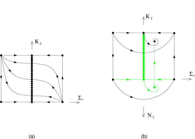
The state space associated with (74) is the product set ${\cal B}\times\left[0,1\right]$, where ${\cal B}$ is the state space of the Bianchi type II LRS cosmologies (or type I, in the case $N_{3}=0$), associated with the subsystem of (74a)-(74b). In this representation the null sphere is replaced by the single geodesic variable $K_{3}$, with $0\leq K_{3}\leq 1$. The remaing two geodesic variables are given by (72). We refrain from giving the various equilibrium points and their eigenvalues. Instead we give the three-dimensional extended state space of (74) in figure 3b and the two-dimensional invariant set $N_{3}=0$ in figure 3a. In figure 3b we have simply shown the skeleton of the state space, i.e. the equilibrium points and the various heteroclinic orbits that join the equilibrium points. The figures depict the situation when $\tfrac{2}{3}<\gamma<2$ since there are no bifurcations for this interval. The sources and sinks can be deduced from the figures. A detailed picture of the orbits in the gravitational state space $K_{3}=0$ is given in WE (see figure 6.5). We note that the orbits in the invariant set $K_{3}=1$ are identical to those with $K_{3}=0$. Knowing the orbits in $K_{3}=0$ and $K_{3}=1$, one can visualize the structure of the geodesic submanifolds – they are vertical surfaces of the form $\left\{\Gamma\right\}\times\left[0,1\right]$, where $\Gamma$ is an orbit in the subset $K_{3}=0$.

Figure 3.: The dynamics of the extended system of equations for (a) Bianchi type I LRS models and (b) Bianchi type II LRS models.

Comments on Bianchi type IX models

It was recognized a long time ago that the oscillatory approach to the past or future singularity of Bianchi IX vacuum models, the so-called Mixmaster attractor, displays random features, see e.g. Belinskii et al. [9], and hence is a potential source of chaos. This behavior is also expected in non-vacuum Bianchi models with various matter sources (see section 6.4.1 in WE and references therein). Numerical studies of the governing equations of vacuum Bianchi IX models toward the initial singularity have shown that the variables $\Sigma_{\pm}$ and the $N_{\alpha}$ remain bounded. These studies have also shown that the projection of the orbits onto the $\Sigma_{\pm}$-plane is given, at least to a high accuracy, by the Kasner map (see WE, section 11.4.2). The transition between two different Kasner states is described by a vacuum Bianchi type II orbit except when the Kasner state is close to an LRS Kasner model where this approximation is no longer valid. When discussing the Mixmaster attractor, one is usually discussing individual orbits. Thus a corresponding discussion for the extended system implies a discussion about the Bianchi type IX geodesic submanifold. Precisely as an individual Bianchi type IX orbit can be approximated by a sequence of Bianchi type II orbits, one can approximate a type IX geodesic submanifold with a sequence of type II geodesic submanifolds. The stable equilibrium points within the type II geodesic submanifold reside in the type I geodesic boundary submanifold of these models and correspond to geodesics in the 1,2 or 3 directions, modulo sign, depending on the particular Kasner point.

We will only consider such sequences of Kasner states for which the Kasner models are not close to any LRS models. As the evolution progresses, the $\tau$-time that the system spends close to a Kasner state, a so-called Kasner epoch, becomes successively longer and should thus be well described by the appropriate equilibrium point. If we assume that during a certain Kasner epoch the qualitative behavior of a geodesic is given by the stable equilibrium point of the extended system of equations for these models, we can extend the Kasner map to include the stable direction of the geodesic. Since we are excluding the LRS Kasner models there will never appear any equilibrium sets as they only when $\varphi$ is a multiple of $\pi/3$. The direction of stability, modulo sign, is given in table 4 as a function of $\varphi$. These results follow from the general stability of the equilibrium points given in table 1, by changing the signs of the eigenvalues since the models are approaching the the initial singularity, i.e. $\tau\rightarrow-\infty$.

Range of $\varphi$	Stable geodesic direction
$0<\varphi<2\pi/3$	$1$
$2\pi/3<\varphi<4\pi/3$	$3$
$4\pi/3<\varphi<2\pi$	$2$

Table 4.: The stable geodesic direction for the geodesics for a particular Kasner epoch for different $\varphi$’s. By assumption we exclude all the LRS Kasner models, i.e. models when $\varphi$ is a multiple of $\pi/3$.

Starting with a geodesic whose tangent vector satisfies $K_{1},K_{2},K_{3}\geq 0$ in a given Kasner epoch with $0<\varphi_{\text{ini}}<\pi/3$, the stable geodesic direction is the 1–direction. The system then evolves, according to the Kasner map, into a state with $\tfrac{\pi}{3}<\varphi_{\text{fin}}<\pi$. Depending on the initial value $\varphi_{\text{ini}}$, the stable geodesic direction can either stay the same ($\text{arccos}\left(\tfrac{13}{14}\right)<\varphi_{ini}<\tfrac{\pi}{3}$) or change to the 2-direction ($0<\varphi_{\text{ini}}<\text{arccos}\left(\tfrac{13}{14}\right)$). This process is then repeated as the state changes again. This extended Kasner map is shown in figure 4. In the figure, a whole sequence of Kasner states is also shown where the stable geodesic directions are given by the sequence $1,1,2,2,1,3$.

Figure 4.: The extended Kasner map including the stable geodesic directions. The sequence of Kasner states depicted has the following sequence of stable geodesic directions: 1,1,2,2,1,3.

The above discussion of the behavior of geodesics toward the Mixmaster singularity is based on the assumption that as the system changes from one Kasner epoch to another, the geodesics are not affected. This means that a tangent vector to the geodesic with $K_{1,2,3}>0$ can never evolve into a tangent vector with one or more of the $K_{\alpha}$’s negative.

This assumption is rather crude since the change of Kasner epochs is approximately described by a vacuum Bianchi type II orbit, for which the geodesic equations, if viewed as separate from the field equations, are non-autonomous. Taking this into account limits the predictability of the “extended Kasner map” in that it cannot predict if a geodesic evolves in the positive or negative direction of the stable geodesic direction. We also note that it is only in $\tau$-time that the system spends longer and longer time in each Kasner epoch. In synchronous time, the interval becomes shorter and shorter.

From the above discussion, it is expected that there will be some kind of geodesic chaos in the development toward the initial and final singularity. To substantiate this, one would need, in addition to further analytical results, careful numerical studies. We believe that the extended system of equations, as presented in this paper, may be very well suited for such an analysis. The next step would be to study the extended system of equations for Bianchi type II vacuum models.

5 Temperature distribution

In this section we describe how the extended system of equations (62)-(64), together with the decoupled energy equation (16), can be used to study the temperature of the CMB in an SH universe. We regard the photons of the CMB as a test fluid, i.e. one which is not a source of the gravitational field. It is possible to include the effect of the CMB photons on the gravitational field by considering two non-interacting fluids, radiation and dust, using the approach of Coley & Wainwright [10]. We will not do this since the effects of the radiation fluid is not expected to change our results significantly. To obtain the present temperature of the CMB, the photon energies are integrated along the null geodesics connecting points of emission on the surface of last scattering to the event of observation at the present time. To simplify the discussion, it is assumed that the decoupling of matter and radiation takes place instantaneously at the surface of last scattering. The matter of the background cosmological model is assumed to be described by dust, i.e. $p=0$.

By the following simple argument we can approximate the interval of dimensionless time, $\Delta\tau$, that has elapsed from the event of last scattering until now. If the radiation is thermally distributed, its energy density $\mu_{\rm r}$, as derived from the quantum statistical mechanics of massless particles, satisfies $\mu_{\rm r}\propto T^{4}$ where $T$ is the temperature of the radiation (see Wald [11], page 108). A non-tilted radiation fluid satisfies $\mu_{\rm r}\propto{\rm exp}(-4\tau)$, which implies

$$\frac{T_{\rm o}}{T_{\rm e}}\approx e^{-\Delta\tau}\ .$$ (80)

Here $T_{\rm o}$ and $T_{\rm e}$ are the temperature at the present time and at the surface of last scattering respectively. Assuming that the process of last scattering took place when $T_{\rm e}\approx 3000$ K, and that the mean temperature of the CMB today is $T_{\rm o}\approx 3$, it follows that $\Delta\tau\approx 7$. This corresponds to a redshift of about $z\approx 1100$.

The temperature of the CMB can now be found as follows. Introduce a future-pointing null vector ${\bf k}$ which is tangent to a light ray at a point on the CMB sky. The current observed temperature $T_{\rm o}$ of the CMB is given by (see, for example, Collins & Hawking [3], page 313 )

$$\frac{T_{\rm o}}{T_{\rm e}}=\frac{\left(u_{a}k^{a}\right)_{\rm o}}{\left(u_{a}k^{a}\right)_{\rm e}}=\frac{{\cal E}(t_{\rm o})}{{\cal E}(\tau_{\rm e})}\ .$$ (81)

From Eqs. (16) and (30) it follows that

$$T_{\rm o}=T_{\rm e}\exp\left[-\int_{\tau_{\rm e}}^{\tau_{\rm o}}\left(1+\Sigma_{\alpha\beta}(\tau)K^{\alpha}(\tau)K^{\beta}(\tau)\right)d\tau\right]\ .$$ (82)

This formula gives the temperature at time $\tau=\tau_{0}$ in the direction specified by the direction cosines $K_{\alpha}(\tau_{0})$. We introduce angles $\theta,\varphi$ by

$$K_{1}(\tau_{0}) =\sin\theta\cos\varphi\ ,$$ (83)

$$K_{2}(\tau_{0}) =\sin\theta\sin\varphi\ ,$$ (84)

$$K_{3}(\tau_{0}) =\cos\theta\ ,$$ (85)

to describe positions on the celestial sphere. Note that to obtain a correspondence with the spherical angles defining the direction in which an observer measures the temperature of the CMB, one has to make the transformation $\theta\rightarrow\pi-\theta$, $\varphi\rightarrow\varphi+\pi$. In this way, $T_{\rm o}$ is a function of the angles $\theta$ and $\varphi$, i.e.

$$T_{\rm o}=T(\theta,\varphi)\ ,$$ (86)

which we call the temperature function of the CMB.

The anisotropy in the CMB temperature can be described using multipole moments (see for example Bajtlik et al. [5]). The fluctuation of the CMB temperature over the celestial sphere is written as a spherical harmonic expansion,

$$\frac{\Delta T}{T}\left(\theta,\varphi\right)=\frac{T(\theta,\varphi)-T_{\rm av}}{T_{\rm av}}=\sum_{l=1}^{\infty}\sum_{m=-l}^{l}a_{lm}Y_{lm}\left(\theta,\varphi\right)\ ,$$ (87)

where $T_{\rm av}$ is the mean temperature of the CMB sky. The coefficients $a_{lm}$ are defined by

$$a_{lm}=\iint\limits_{S^{2}}\frac{\Delta T}{T}\left(\theta,\varphi\right)Y^{*}_{lm}\left(\theta,\varphi\right)d\Omega\ ,$$ (88)

where * denotes complex conjugation, and the integral is taken over the 2-sphere (see for example Zwillinger [12], pages 492-493). The multipole moments, describing the anisotropies in a coordinate independent way, are defined as

$$a_{l}=\left(\sum_{m=-l}^{l}\left|a_{lm}\right|^{2}\right)^{1/2}\ .$$ (89)

The dipole, $a_{1}$, is interpreted as describing the motion of the solar system with respect to the rest frame of the CMB. Therefore, the lowest multipole moment that describes true anisotropies of the CMB temperature is the quadrupole moment, $a_{2}$. Current observations provide an estimate for $a_{2}$ as well as for the octupole moment $a_{3}$ (see Stoeger et al. [13]).

In order to compute $T(\theta,\varphi)$ and the multipole moments $a_{2}$ and $a_{3}$ for a particular cosmological model, one has to specify the dimensionless state, ${\bf x}(\tau_{\rm o})={\bf x}_{\rm o}$, of the model at the time of observation, $\tau_{\rm o}$, and the direction of reception $K_{\alpha}(\tau_{\rm o})$, which determines the angles $\theta$ and $\varphi$ on the celestial sphere via (84). The solution ${\bf x}(\tau)$, $K_{\alpha}(\tau)$ of the extended system of equations (62) and (63), determined by the initial conditions ${\bf x}(\tau_{\rm o})$ and $K_{\alpha}(\tau_{\rm o})$, is substituted in (82), which determines the temperature function $T\left(\theta,\varphi\right)$. The multipoles $a_{2}$ and $a_{3}$ are then calculated by integrating over the 2-sphere (see (88) and (89)). In this way the multipole moments can be viewed as functions defined on the dimensionless gravitational state space, with the time elapsed $\Delta\tau$ since last scattering as an additional parameter:

$$a_{2}=a_{2}({\bf x}_{\rm o};\Delta\tau)\ ,\quad a_{3}=a_{3}({\bf x}_{\rm o};\Delta\tau)\ .$$ (90)

The extended equations can be used in three ways to obtain information about $T(\theta,\varphi)$ and the multipoles $a_{2}$ and $a_{3}$, as follows.

1. Apply dynamical systems methods to the extended equations to obtain qualitative information about the null geodesics and the shear, and hence about the temperature pattern of the CMB.

2. Linearize the extended equations about an FL model, and if possible solve them to obtain approximate analytical expressions for $T(\theta,\varphi)$, $a_{2}$ and $a_{3}$, which are then valid for $\Sigma<<1$.

3. Use the full non-linear extended equations to do numerical simulations, calculating $T(\theta,\varphi)$, $a_{2}$ and $a_{3}$ for a given point ${\bf x}_{\rm o}$ in the gravitational state space, not necessarily satisfying $\Sigma_{\rm o}<<1$. As described above, one calculates the value of $T\left(\theta,\varphi\right)$ at each point of a grid covering the celestial sphere and then integrates numerically over the sphere to obtain $a_{2}$ and $a_{3}$.

One can use the observational bounds on $a_{2}$ and $a_{3}$, together with the results of ii) and iii) above, to determine bounds on the anisotropy parameters associated with the shear and the Weyl curvature, $\Sigma_{\rm o}$ and ${\cal W}_{\rm o}$. A necessary condition for the model to be close to FL at the time of observation is that $\Sigma_{\rm o}$ and ${\cal W}_{\rm o}$ are small (see Nilsson et al. [14]).

We are in the process of applying the above methods to SH models of various Bianchi group types. Preliminary results on Bianchi VII₀ models are given in Nilsson et al. [14], where it is shown that the observational bounds on $a_{2}$ and $a_{3}$ do not necessarily imply that the Weyl parameter ${\cal W}_{\rm o}$ is small. Thus, an almost isotropic CMB temperature does not imply an almost isotropic universe. An advantage of the above methods is that they are not restricted to those Bianchi types that are admitted by the FL models. For example, we are studying the diagonal class B models of Bianchi type VI_h as described by (2 A). The current state ${\bf x}_{\rm o}$ can be described by $\Sigma_{\rm o}$, $k$ and $\Omega_{\rm o}$, and so the expression for the quadrupole has the general form

$$a_{2}=a_{2}(\Sigma_{{\rm o}},k,\Omega_{\rm o};\Delta\tau)\ .$$ (91)

When one uses the method ii) and linearizes about the open FL model ($\Sigma_{\rm o}=k=0$), one obtains a formula of the form

$$a_{2}\approx\Sigma_{\rm o}I_{2}(\Omega_{\rm o};\Delta\tau)+kJ_{2}(\Omega_{\rm o};\Delta\tau)\ ,$$ (92)

where $I_{2}$ and $J_{2}$ are expressed as integrals. This formula, which is valid for $\Sigma_{\rm o}<<1$ and $k<<1$, leads to bounds on the shear parameter $\Sigma_{\rm o}$ that are much weaker than those obtained in Bianchi types I and V (see Lim et al. [15]). This result shows that the bounds obtained for the anisotropy parameters in Bianchi type I and V models (see, for example Bajtlik et al. [5]), which seem to have been taken for granted as being typical, are misleading.

6 Discussion

In this paper we have shown that in the case of spatially homogeneous models, the field equations can be augmented with the geodesic equations, producing an extended set of first-order evolution equations whose solutions describe not only the evolving geometry but also the structure of the geodesics. Examples of the dynamics of geodesics in some self-similar models, and in a simple non-self-similar model, in order to show the predictive power of the approach, were given. We also made some conjectures about the qualitative behavior of geodesics towards the initial Mixmaster singularity in Bianchi IX models by considering the geodesics structure of the Kasner models. In light of the chaotic nature of the Mixmaster singularity, it is expected that the geodesics will also have some sort of chaotic behavior. To confirm these speculations, we point out that further analytic studies and thorough numerical investigations are needed. We believe that the formulation of the combined field equations and geodesic equations of this paper is very well suited for this purpose.

The most physically interesting aspect of the extended set of equations is the possibility of shedding light on one of the fundamental questions concerning the CMB, namely, does a highly isotropic CMB temperature imply that the universe can accurately be described by an FL model? As mentioned in section 5, the preliminary indications are that the situation is less clear-cut than was previously thought.

We now conclude by listing some related research topics. One can easily generalize the present formalism to spatially self-similar models and it is also easy to include other sources, e.g. , two non-interacting fluids, a cosmological constant, or magnetic fields. It should also be possible to extend the system to include polarization. It would also be interesting if the current formulation could be generalized to facilitate a study of the temperature of the CMB for density perturbed models or models with closed topologies.

A Obtaining the geodesics

For many physical purposes in SH cosmology, it is sufficient to know the tangent vector field $\bf k$ of the geodesics. Nevertheless, it might be interesting to find the geodesics themselves. To do so, spacetime coordinates $x^{\mu}$ ($\mu=0,1,2,3$) must be introduced. Once this is done, a geodesic can locally be described as a curve $x^{\mu}(\lambda)$, where $\lambda$ is the affine parameter of the geodesic. With an SH geometry, it is natural to adapt the coordinates to the structure imposed by the SH condition. Expressed in terms of coordinates, the orthonormal frame can then be written as

$${\bf e}_{0}=N(t)^{-1}\,(\mbox{\boldmath$\partial$}_{t}-{N}{}^{i}(t,{\bf x})\,{\bf E}_{i}({\bf x}))\ ,\quad{\bf e}_{\alpha}={e}_{\alpha}{}^{i}(t)\,{\bf E}_{i}({\bf x})\ ,$$ (A1)

where $N$ and $\vec{\bf N}=N{}^{i}{\bf E}_{i}$ are the lapse function and the shift vector field respectively (for restrictions on the shift vector field, see Jantzen & Uggla [16]). The spatial frame $\{{\bf E}_{i}({\bf x})\}$, where $i=1,2,3$ (in this appendix, and only here, latin indices $i,j,k...=1,2,3$ denote spatially homogeneous time independent frame indices since it is only here that this type of frame is used), tangent to each hypersurface, is not only invariant under the action of the Bianchi symmetry group but has structure or commutator functions ${C}{}^{k}\!_{ij}$ which are constants throughout the spacetime, defined by

$$\left[\,{\bf E}_{i},{\bf E}_{j}\,\right]={C}^{k}\!_{ij}\,{\bf E}_{k}\ .$$ (A2)

It is possible to construct the orthonormal frame explicitly in terms of local coordinates $\{t,x^{i}\}$ ($i=1,2,3$) adapted to the SH hypersurfaces. The spatial frame $\{{\bf E}_{i}\}$ is characterized by the Lie dragging condition ${\cal L}_{{\boldsymbol{\partial}_{t}}}{\bf E}_{i}=0$ which implies the time independent local coordinate expression ${\bf E}_{i}={E}_{i}{}^{j}(x^{k})\,{\boldsymbol{\partial}}_{j}$ for the invariant spatial frame. Explicit coordinate expressions for ${E}_{i}{}^{j}(x^{k})$ follow from the representation of the left invariant vector fields in canonical coordinates of the second kind in Jantzen [17, 18]. The relation between the orthonormal frame components of the tangent vector field to the geodesics and its corresponding coordinate components yields the relations

$$\frac{d\lambda}{d\tau} = (H{\cal E})^{-1}\ ,$$ (A4)

$$\frac{dx^{i}}{d\tau} = \sum_{j}[-N^{j}(\tau,{\bf x})+H^{-1}(\sum_{\alpha}K^{\alpha}(\tau)e_{\alpha}{}^{j}(\tau))]E_{j}{}^{i}({\bf x})\ ,$$ (A5)

where the $K^{\alpha}$ are the energy-normalized components of the geodesic tangent vector field. Here one can choose an automorphism adapted shift in order to set certain components of $e_{\alpha}{}^{j}(\tau)$ to zero, see Jantzen & Uggla [16]. One usually sets the shift to zero. In this latter case one has to add equations governing some of the $e_{\alpha}{}^{j}(\tau)$ components. These are obtained from the commutator relations and are consequences of the zero-shift gauge. We will not do this for the general case. Instead we will look at an example.

1 An example: Non-tilted class A models with zero shift

In this case, with zero shift, equation (A) becomes

$$d\lambda/d\tau =(H{\cal E})^{-1}\ ,$$ (A6)

$$dx^{i}/d\tau =\sum_{\alpha}H^{-1}K^{\alpha}e^{-{\beta_{\alpha}}}E_{\alpha}{}^{i}(x)\ ,$$ (A7)

where $e_{\alpha}\!^{j}=\delta_{\alpha}^{j}{\rm e}^{-\beta_{\alpha}}$. The commutator equations (see Jantzen & Uggla [16] or WE, chapter 10) yields

$$d\beta_{1,2}/d\tau =1+\Sigma_{+}\pm\sqrt{3}\Sigma_{-}\ ,$$ (A8)

$$d\beta_{3}/d\tau =1-2\Sigma_{+}\ .$$ (A9)

The next step is to introduce $H^{-1}{\rm e}^{-\beta_{\alpha}}$ as new variables, but note that they are not independent of $N_{\alpha}$ (see WE, chapter 10). This results in the complete extended system of equations, which is necessary in order to obtain the individual geodesics.

REFERENCES

- [1] Wainwright, J. and Ellis, G. F. R. (1997). Dynamical systems in cosmology (Cambridge University Press, Cambridge).
- [2] Ellis, G. F. R. and MacCallum, M. A. H. (1969). Commun. Math. Phys. 12, 108.
- [3] Collins, C. B. and Hawking, S. W. (1973). Mon. Not. Roy. Astr. Soc. 162, 307.
- [4] Barrow, J. D., Juszkiewicz, R., and Sonoda, D. H. (1983). Nature 309, 397.
- [5] Bajtlik, S., Juszkiewicz, R., Proszynski, M., and Amsterdamski, P. (1985). Astrophys. J. 300, 463.
- [6] Doroshkevich, A. G., Lukash, V. N., and Novikov, I. D. (1975). Sov. Astronomy 18, 554.
- [7] Wainwright, J., Hancock, M. J., and Uggla, C. (1999). Class. Quant. Grav. 16, 2577.
- [8] Collins, C. B. and Stewart, J. M. (1971). Mon. Not. Roy. Astr. Soc. 153, 419.
- [9] Belinskii, V. A., Khalatnikov, I. M., and Lifschitz, E. M. (1970). Adv. Phys. 19, 525.
- [10] Coley, A. A. and Wainwright, J. (1992). Class. Quant. Grav. 9, 651.
- [11] Wald, R. M. (1984). General relativity (University of Chicago Press, Chicago).
- [12] Zwillinger, D. (1996). CRC Standard mathematical tables and formulae (CRC Press, Boca Raton).
- [13] Stoeger, W. R., Araujo, M. E., and Gebbie, T. (1997). Astrophys. J. 476, 435.
- [14] Nilsson, U. S., Uggla, C., and Wainwright, J. (1999). Astrophys. J. Lett. 522, L1.
- [15] Lim, W. C., Nilsson, U., and Wainwright, J. (1999). “The temperature of the cosmic microwave background in Bianchi VIh universes”, in preparation.
- [16] Jantzen, R. T. and Uggla, C. (1999). J. Math. Phys. 40, 353.
- [17] Jantzen, R. T. (1979). Commun. Math. Phys. 64, 211.
- [18] Jantzen, R. T. (1984). “Spatially homogeneous dynamics: a unified picture”, In Ruffini, R. and Melchiorri, F. editors, Proc. Int. Sch. Phys. ’E Fermi Course LXXXVI on ’Gamov cosmology, page 61, (Amsterdam:North Holland).