A new numerical method for constructing quasi-equilibrium sequences of irrotational binary neutron stars in general relativity

Abstract

We propose a new numerical method to compute quasi-equilibrium sequences of general relativistic irrotational binary neutron star systems. It is a good approximation to assume that (1) the binary star system is irrotational, i.e. the vorticity of the flow field inside component stars vanishes everywhere (irrotational flow), and (2) the binary star system is in quasi-equilibrium, for an inspiraling binary neutron star system just before the coalescence as a result of gravitational wave emission. We can introduce the velocity potential for such an irrotational flow field, which satisfies an elliptic partial differential equation (PDE) with a Neumann type boundary condition at the stellar surface. For a treatment of general relativistic gravity, we use the Wilson–Mathews formulation, which assumes conformal flatness for spatial components of metric. In this formulation, the basic equations are expressed by a system of elliptic PDEs. We have developed a method to solve these PDEs with appropriate boundary conditions. The method is based on the established prescription for computing equilibrium states of rapidly rotating axisymmetric neutron stars or Newtonian binary systems. We have checked the reliability of our new code by comparing our results with those of other computations available. We have also performed several convergence tests. By using this code, we have obtained quasi-equilibrium sequences of irrotational binary star systems with strong gravity as models for final states of real evolution of binary neutron star systems just before coalescence. Analysis of our quasi-equilibrium sequences of binary star systems shows that the systems may not suffer from dynamical instability of the orbital motion and that the maximum density does not increase as the binary separation decreases.

]

I Introduction

At the beginning of the next century, advanced gravitational wave detectors (LIGO/VIRGO/TAMA/GEO; [1]) will provide us with signals from coalescing binary neutron star systems. According to the type of compact objects involved (for example, black holes/neutron stars, isolated/binary objects, solar mass/super massive objects), various theoretical methods have been developed or are under development to predict and interpret gravitational wave signals which will be observed. Compact binary systems of solar mass sizes are also promising sources of $\gamma-$ ray bursts or r-process nuclei. These are important issues of recent astrophysics (see for example [2] and references therein).

When we consider the final evolutionary stage of the binary neutron star (BNS) as a result of gravitational wave emission, it is necessary to solve the internal structure of the neutron star (NS) at the late inspiraling stage as well as the early stage of merging, since the size of the star is comparable to the separation of the two neutron stars. In this case, (1) tidal deformation of a component star, (2) the general relativistic effect on the orbital motion, and (3) the general relativistic effect on the internal structure of a star are coupled to affect the physics of the binary system. Such finite size effects are not negligible for the last ${\cal N}\mathrel{\raise 1.29167pt\hbox{$<$}\mkern-14.0mu\lower 2.58334pt\hbox{$\sim$}}10$ cycles of the inspiraling phase just before coalescence [2].

According to the scenario of the final evolution of the close BNS [3], the flow field inside component stars just prior to coalescence becomes irrotational, i.e. a vorticity seen from the non-rotating observer’s frame vanishes just prior to coalescence. This irrotational flow is realized because (1) the viscosity of neutron star matter is too weak to synchronize the spins of the component stars and the orbital angular velocity of the binary system during the evolution, and (2) the initial spin period of each NS is much larger than the final orbital period of the BNS. It is on precisely this stage of the binary evolution that we focus in the present paper.

Full 3D numerical simulations are most promising to investigate such final phases of BNS systems. Numerical methods for fully dynamical 3D GR computations of BNS’s are developing rapidly (see for example [4, 5, 6]). However it is still difficult to perform simulations over the whole ${\cal N}\mathrel{\raise 1.29167pt\hbox{$<$}\mkern-14.0mu\lower 2.58334pt\hbox{$\sim$}}10$ cycles of the inspiraling BNS because there remain some technical problems to overcome for newly developed 3D GR codes, such as, maintaining stability and accuracy of numerical schemes and restrictions on the computational power of present computers. Recently, Shibata has succeeded in developing a new numerical method to compute dynamical evolution of the space-time and compact object(s) such as a single NS or a BNS system in a stable manner [6]. Therefore simulations over several orbital periods of BNS will be performed in the near future. However, even after that, it is desirable to have totally different and supplementary methods to investigate such systems to test the reliability of the theory based on numerical methods.

One of promising alternative ways to tackle this problem is to compute quasi-equilibrium sequences of BNS configurations. Since the time scale of evolution as a result of gravitational wave (GW) emission is longer than the time scale of the orbital motion even at this stage, quasi-equilibrium is a good approximation for a realistic BNS system [7]. Therefore, a quasi-equilibrium sequence with a constant rest mass constructed by changing the binary separation could be considered as an evolutionary sequence of such an inspiraling BNS system. Also, quasi-equilibrium configurations will give accurate initial conditions for the future 3D GR dynamical computations. Therefore, it is important to develop a numerical method to compute quasi-equilibrium configurations of close BNS’s.

In this paper we introduce a new numerical method to compute quasi-equilibrium configurations of irrotational BNS systems. It is a straightforward extension of the computational method used for the Newtonian irrotational binary systems developed by the present authors [8]. We discuss the formulation of the problem separately for (1) the gravitation part (the Einstein equations) and (2) the fluid part (the NS, i.e., the equation of motion, the continuity equation, the equation of state (EOS) and so on). As the first step of the extension to general relativistic strong gravity, a simplified system of the Einstein equations is employed. We use the formulation developed by Wilson and Mathews [9] and Baumgarte et al. [10], in which the metric is decomposed into (3+1) form and its spatial part is assumed to be conformally flat. For the fluid part, we solve the equations for irrotational flow whose formulation in GR has been developed by Shibata [11] and Teukolsky [12] (see also [13]). Our new computational code reproduces results of several independent computations previously made for GR co-rotating BNS’s and Newtonian irrotational binary systems with reasonable accuracy. The convergence test of the numerical scheme is shown as well. Using this new code, we have constructed quasi-equilibrium sequences of irrotational BNS’s with constant rest mass, which approximate the final evolutionary track of a realistic BNS as a result of GW emission. Analysis of our quasi-equilibrium sequences of binary star systems suggests that the systems may not suffer from dynamical instability of the orbital motion and that the maximum density does not increase as the binary separation decreases.

This paper is organized as follows. In section II we review the formulation for quasi-equilibrium irrotational binary systems in GR and derive the basic equations. In section III, we present the new numerical method for solving them. In section IV, we present several comparisons with other computations, a convergence test of the new numerical scheme and the results for the binary configurations and quasi-equilibrium sequences. In section V, we discuss the validity of the present results and future prospects.

II Review of the formulation of the problem

A Quasi-equilibrium irrotational binary systems in GR: Summary of the assumptions and of the formulation

Because of the finite size effect of stars in a close binary system, it is necessary to solve for the structures of the stars without approximation for the last ${\cal N}\mathrel{\raise 1.29167pt\hbox{$<$}\mkern-14.0mu\lower 2.58334pt\hbox{$\sim$}}10$ cycles of the inspiraling phase just before coalescence. In general, the binary system cannot be in equilibrium in GR since GW carry angular momentum and energy away to infinity. However, the quasi-equilibrium approximation is well fulfilled since the time scale of evolution due to GW emission is longer than that of the orbital period even just before coalescence [7]. In this situation, we can expect that (A) there exists an approximate Killing vector $\vec{\ell}$ expressing this symmetry of the space-time and the fluid. Moreover, it has been pointed out by Kochanek and by Bildsten & Cutler [3] that (B) the flow fields of binary stars just before coalescence become irrotational, because (i) the viscosity of the neutron star matter is too weak to synchronize the spins and the orbital angular velocity by the time of merging and (ii) the initial spin angular velocity of each component star is negligible compared to the final orbital angular velocity.

To construct realistic BNS’s in quasi-equilibrium, the above two properties (A) and (B) should be implemented in the formulation of the basic equations. Strictly speaking, it is impossible to assume the property (A) in exact GR, because there arises GW emission from the source to the asymptotically flat region. This implies that there is no unique way to formulate properly an approximation which fulfills the property (A) for the Einstein equations. However, several authors have developed formulations for BNS’s in quasi-equilibrium. The formulation for the first and second post-Newtonian approximations (1PN/2PN, respectively) have been developed and co-rotating quasi-equilibrium configurations of BNS’s in the 1PN approximation have been calculated [14]. Also, the Wilson–Mathews formulation has been implemented by several authors [9, 10] to express quasi-equilibrium BNS’s as well as space-time around them. In this paper we use the Wilson–Mathews formulation to express the gravitational field. For the fluid, the property (B) is implemented by introducing the velocity potential and assuming the barotropic flow. The property (A) is imposed by decomposing the variables into the direction of the Killing vector $\vec{\ell}$ and the spatial direction [11, 12, 13].

Consequently the basic equations we use in this paper are identical with those used by Bonazzola, Gourgoulhon and Marck [15] and by Marronetti, Mathews and Wilson [16]. We will summarize the formulation and the basic equations below. Geometrical units with $G=c=1$ are used throughout this paper. Latin indices run from 1 to 3, whereas Greek indices run from 0 to 3.

B Formulation for the gravitational field

We adopt the ADM decomposition for the convenience of numerical computations. The metric is written as,

$$ds^{2} = g_{\mu\nu}dx^{\mu}dx^{\nu}$$ (1)

$$= -\alpha^{2}dt^{2}+\gamma_{ij}\left(dx^{i}-\omega^{i}dt\right)\left(dx^{j}-\omega^{j}dt\right),$$ (2)

where $g_{\mu\nu}$, $\alpha$, $\omega^{i}$ and $\gamma_{ij}$ are the 4-metric, the lapse function, the shift vector and the 3-metric on a 3D spatial hypersurface $\Sigma_{t}$, respectively. The unit normal to $\Sigma_{t}$ is written as

$$n^{\mu}=\left(\frac{1}{\alpha},\frac{\omega^{i}}{\alpha}\right)\quad{\rm and}\quad n_{\mu}=\left(-\alpha,0,0,0\right),$$ (3)

and $\gamma_{\mu\nu}$ is defined as

$$\gamma_{\mu\nu}=g_{\mu\nu}+n_{\mu}n_{\nu}.$$ (4)

By using the (3+1) formalism, the Einstein equations are decomposed into constraint equations and evolution equations. The Hamiltonian constraint and the momentum constraints are, respectively,

$$R-K_{ij}K^{ij}+K^{2}=16\pi\rho_{H},$$ (5)

$$D_{j}K^{ij}-D^{i}K=8\pi j^{i},$$ (6)

where the source terms $\rho_{H}$ and $j^{\sigma}$ are defined by

$$\rho_{H}=n^{\mu}n^{\nu}T_{\mu\nu},$$ (7)

$$j^{\sigma}=-\gamma^{\sigma}_{~{}\mu}n_{\nu}T^{\mu\nu}.$$ (8)

Here $R$, $K_{ij}$, $K$, $D_{i}$ and $T_{\mu\nu}$ are the scalar curvature, the extrinsic curvature, the trace part of $K_{ij}$, the covariant derivative with respect to $\gamma_{ij}$, and the stress-energy tensor, respectively.

According to the (3+1) formalism, the 3-metric $\gamma_{ij}$ satisfies the dynamical equations

$${\partial\over\partial t}\gamma_{ij}=-2\alpha K_{ij}-D_{i}\omega_{j}-D_{j}\omega_{i}.$$ (9)

These equations are decomposed into their trace part and trace free parts [18] :

$${\partial\over\partial t}\ln\gamma^{1/2}=-\alpha K-D_{i}\omega^{i},$$ (10)

$$\gamma^{1/3}{\partial\over\partial t}\left(\gamma^{-1/3}\gamma_{ij}\right) = -2\alpha\left(K_{ij}-\frac{1}{3}\gamma_{ij}K\right)$$ (11)

$$-{}D_{i}\omega_{j} - D_{j}\omega_{i}+\frac{2}{3}\gamma_{ij}D_{k}\omega_{k}.$$ (12)

where $\gamma=\det\gamma_{ij}$ and $K=K^{i}_{~{}i}$.

The dynamical equations for $K_{ij}$ are also derived and decomposed into their trace part and trace free parts. We only write the trace part :

$${\partial K\over\partial t}=\alpha R-D^{i}D_{i}\alpha+\alpha K^{2}-\omega^{i}D_{i}K$$ (13)

$$-{}4\pi\alpha\left(3\rho_{H}-S\right),$$ (14)

where $S$ is defined as

$$S=\gamma^{ij}T_{ij}.$$ (15)

The post-Newtonian approach up to the 2PN order admits exact equilibrium states of BNS’s [14]. However, the 2PN equations for gravity require a significant amount of computation. Also, the problem of GR formulation for quasi-equilibrium states has not been settled. To make the problem tractable, we assume that the spatial part of the metric $\gamma_{ij}$ is conformally flat for all the time during the inspiraling stage as follows:

$$\gamma^{-1/3}\gamma_{ij}=f_{ij},$$ (16)

$$\gamma_{ij}=\gamma^{1/3}f_{ij}\equiv\Psi^{4}f_{ij}.$$ (17)

where $f_{ij}$ is the flat space metric and $\Psi$ is a conformal factor [9, 10]. This is a rather strong restriction for the space-time since it is well known that the 3-metric is not conformally flat even for stationary axisymmetric space-time. However, under this assumption, we can compute exactly BNS’s up to the 1PN order and spherically symmetric configurations in full GR. It is also expected that this choice minimizes the gravitational wave content of the (physical) space-time by removing the dynamical or “wave” degrees of freedom from the field. Moreover, since this choice can always be adopted to find initial data without any approximation, our solutions give initial conditions for 3D simulations of BNS coalescence in full GR [17].

For the time slicing condition we choose maximal slicing:

$$K=0,$$ (18)

and we assume that this condition holds for all the time of the evolution

$${\partial K\over\partial t}=0,$$ (19)

although the other evolution equations for $K_{ij}$ are omitted artificially.

From the above assumptions Eqs. (16) – (19), the basic equations for the gravitational field, become as follows. The scalar curvature reduces to

$$R=-8\Psi^{-5}\nabla^{2}\Psi,$$ (20)

where $\nabla^{2}=\nabla^{i}\nabla_{i}=f^{ij}\nabla_{i}\nabla_{j}$ is the Laplacian of flat 3-space. Eqs. (5), (6), (11) and (13) are rewritten as

$$\nabla^{2}\Psi=-\frac{1}{8}\Psi^{-7}\widetilde{K}_{ij}\widetilde{K}^{ij}-2\pi\Psi^{5}\rho_{H},$$ (21)

$$\nabla^{2}\omega^{i}+\frac{1}{3}\nabla^{i}\nabla_{j}\omega^{j}=-2\nabla_{j}\left(\alpha\Psi^{-6}\right)\widetilde{K}^{ij}-16\pi\alpha\Psi^{4}j^{i},$$ (22)

$$\widetilde{K}^{ij}=-\frac{\Psi^{6}}{\alpha}\left(\frac{1}{2}\left(\nabla^{i}\omega^{j}+\nabla^{j}\omega^{i}\right)-\frac{1}{3}f^{ij}\nabla_{k}\omega^{k}\right),$$ (23)

$$\nabla^{2}\left(\alpha\Psi\right)=\alpha\Psi\left(\frac{7}{8}\Psi^{-8}\widetilde{K}_{ij}\widetilde{K}^{ij}+2\pi\Psi^{4}(\rho+2S)\right).$$ (24)

Here we define $\widetilde{K}^{ij}$ as

$$\widetilde{K}^{ij}=\Psi^{10}K^{ij},$$ (25)

and its indices are lowered by the flat metric $f_{ij}$, as $\widetilde{K}_{ij}=f_{ik}f_{jl}\widetilde{K}^{kl}$ . $\nabla_{i}$ is the derivative with respect to the flat metric $f_{ij}$.

To make Eq. (22) more tractable, the shift vector $\omega^{i}$ is decomposed into the sum of a vector and the gradient of a scalar as

$$\omega^{i}=G^{i}-\frac{1}{4}\nabla^{i}B.$$ (26)

Eq. (22) is divided into the following equations for these variables $G^{i}$ and $B$ as,

$$\nabla^{2}G^{i}=-2\nabla_{j}\left(\alpha\Psi^{-6}\right)\widetilde{K}^{ij}-16\pi\alpha\Psi^{4}j^{i},$$ (27)

$$\nabla^{2}B=\nabla_{i}G^{i}.$$ (28)

The basic variables of the gravitational potentials for the actual computation are then $\Psi$, $\alpha$, $G^{i}$ and $B$, and the corresponding equations are Eqs. (21), (24), (27) and (28), together with relations (23) and (26). It should be noted that all of these equations are elliptic type PDEs. We can solve these equations iteratively with appropriate boundary conditions by using a certain computational method, which is described in a later section.

C Formulation for the fluid part

General relativistic irrotational flows have been considered as the extension of the Newtonian case and applied for accretion onto a black hole [19] . The formulation of irrotational flow for inspiraling BNS’s in quasi-equilibrium has been derived independently by Shibata [11] and by Teukolsky [12]. We will follow their formulation.

The energy momentum tensor for a perfect fluid can be written as

$$T_{\mu\nu}=\rho\left(1+\varepsilon+\frac{P}{\rho}\right)u_{\mu}u_{\nu}+Pg_{\mu\nu},$$ (29)

where $\rho$, $\varepsilon$, $P$ and $u_{\mu}$ are the rest mass density, the specific internal energy, the pressure and the 4-velocity, respectively. We assume a polytropic EOS for the fluid

$$P=\left(\Gamma-1\right)\rho\varepsilon=\kappa\rho^{1+1/n},$$ (30)

where $n$ is the polytropic index, $\Gamma=1+1/n$, and $\kappa$ is a constant. We define the relativistic specific enthalpy $h$ as

$$h=1+\varepsilon+\frac{P}{\rho}=1+\kappa\left(n+1\right)\rho^{1/n}.$$ (31)

The conservation equation for the energy momentum tensor

$$\,^{(4)}\nabla_{\mu}T^{\mu}_{\nu}=0,$$ (32)

can be rewritten as Euler’s equation

$$u^{\mu}\,{}^{(4)}\nabla_{\mu}\left(hu_{\nu}\right)+\,^{(4)}\nabla_{\nu}h=0,$$ (33)

where $\,{}^{(4)}\nabla_{\mu}$ is the covariant derivative with respect to $g_{\mu\nu}$. The conservation of rest mass density is written as

$$\,^{(4)}\nabla_{\mu}\left(\rho u^{\mu}\right)=0.$$ (34)

The covariant definition of irrotationality in 4D is

$$\omega_{\mu\nu} = P^{\alpha}_{~{}\mu}P^{\beta}_{~{}\nu}\left(\,{}^{(4)}\nabla_{\beta}u_{\alpha}-\,^{(4)}\nabla_{\alpha}u_{\beta}\right)$$ (35)

$$= \frac{1}{h}\left(\,{}^{(4)}\nabla_{\nu}\left(hu_{\mu}\right)-\,^{(4)}\nabla_{\mu}\left(hu_{\nu}\right)\right)=0,$$ (36)

where $P^{\mu}_{~{}\nu}=g^{\mu}_{~{}\nu}+u^{\mu}u_{\nu}$ is the projection tensor and we have made use of Eq. (33). Thus the quantity $hu_{\mu}$ can be expressed in terms of the gradient of a potential $\Phi$ as

$$hu_{\mu}=\,^{(4)}\nabla_{\mu}\Phi.$$ (37)

In the following, we refer to $\Phi$ as the velocity potential. Then the equation of rest mass conservation (34) is rewritten as

$$\,^{(4)}\nabla^{\mu}\,{}^{(4)}\nabla_{\mu}\Phi=-\,^{(4)}\nabla^{\mu}\left(\ln\frac{\rho}{h}\right)\,^{(4)}\nabla_{\mu}\Phi.$$ (38)

From the normalization condition for the 4-velocity $u_{\mu}u^{\mu}=-1$, we get the following equation for $h$

$$h=\left[-\,^{(4)}\nabla_{\mu}\Phi\,^{(4)}\nabla^{\mu}\Phi\right]^{1/2}.$$ (39)

This is the generalized Bernoulli equation in GR since it is also derived by integrating Euler’s equation (33) as follows,

$$h\left(u^{\mu}\,{}^{(4)}\nabla_{\mu}\left(hu_{\nu}\right)+\,^{(4)}\nabla_{\nu}h\right)$$ (41)

$$=\frac{1}{2}\,^{(4)}\nabla_{\nu}\left(\,{}^{(4)}\nabla_{\mu}\Phi\,^{(4)}\nabla^{\mu}\Phi+h^{2}\right)=0.$$

Now we decompose Eqs. (38) and (39) into the ADM (3+1) form and impose the quasi-equilibrium condition. The quasi-equilibrium condition is implemented by assuming the existence of a timelike Killing vector $\ell^{\mu}$ such that

$$\,^{(4)}\nabla_{\nu}\ell_{\mu}+\,^{(4)}\nabla_{\mu}\ell_{\nu}=0$$ (42)

and

$${\cal L}_{\ell}f=\ell^{\mu}\,{}^{(4)}\nabla_{\mu}f=0$$ (43)

where $f$ denotes a certain fluid variable such as $\rho$, $h$ or $u_{\mu}$. ${\cal L}_{\ell}$ denotes the Lie derivative along $\ell^{\mu}$. Since we have assumed a polytropic EOS and irrotational flow, the number of independent fluid variables is two, i.e. the velocity potential $\Phi$ and, for example, the density $\rho$. Note however that not $\Phi$ but its gradient is the fluid variable. Therefore, the following relation holds

$${\cal L}_{\ell}(hu)={\cal L}_{\ell}(d\Phi)=d({\cal L}_{\ell}\Phi)=0,$$ (44)

that is,

$${\cal L}_{\ell}\Phi=\ell^{\mu}\,{}^{(4)}\nabla_{\mu}\Phi=-C$$ (45)

where $C$ is a positive ‘global’ constant on the fluid.

Performing the (3+1) decomposition of Eqs. (38) and (39), and imposing the quasi-equilibrium conditions (43) and (45), we have the following basic equations for irrotational binary systems, respectively [11, 12],

$$D^{i}D_{i}\Phi - B^{i}D_{i}\frac{\lambda}{\alpha^{2}}-\frac{\lambda K}{\alpha}$$ (46)

$$= -\left(D^{i}\Phi-\frac{\lambda}{\alpha^{2}}B^{i}\right)D_{i}\ln\frac{\alpha\rho}{h},$$ (47)

$$h^{2}=\frac{\lambda^{2}}{\alpha^{2}}-D_{i}\Phi D^{i}\Phi.$$ (48)

Here, $B^{i}$ is a rotating shift vector defined as

$$\ell^{\mu}=\alpha n^{\mu}+B^{\mu},\qquad B^{\mu}=-\omega^{\mu}+\Omega\xi^{\mu},$$ (49)

where $\xi^{\mu}$ is the generator of rotations about the rotation axis of the binary. $\lambda$ is defined as

$$\lambda=C+B^{j}D_{j}\Phi.$$ (50)

Using the quasi-equilibrium conditions Eqs. (43) and (45), we obtain the following expressions for the normal derivatives of a scalar quantity $f$ and the velocity potential $\Phi$,

$$n^{\mu}\,{}^{(4)}\nabla_{\mu}f = \frac{1}{\alpha}\left(\ell^{\mu}-B^{\mu}\right)\,^{(4)}\nabla_{\mu}f$$ (51)

$$= -\frac{1}{\alpha}B^{i}D_{i}f,$$ (52)

and

$$n^{\mu}\,{}^{(4)}\nabla_{\mu}\Phi = \frac{1}{\alpha}\left(\ell^{\mu}-B^{\mu}\right)\,^{(4)}\nabla_{\mu}\Phi$$ (53)

$$= -\frac{1}{\alpha}\left(C+B^{i}D_{i}\Phi\right)=-\frac{\lambda}{\alpha}.$$ (54)

The boundary condition for the velocity potential equation is derived as follows from the fact that the spatial fluid velocity on the stellar surface flows along the stellar surface on each 3D spatial hypersurface. We decompose $u^{\mu}$ as

$$u^{\mu}=u^{0}\left(\ell^{\mu}+V^{\mu}\right).$$ (55)

and assume that $V^{\mu}$ is a spatial vector, $n_{\mu}V^{\mu}=0$. By using $V^{\mu}$, the boundary condition is expressed as

$$\left.V^{i}D_{i}\rho\right|_{\rm surf}=0.$$ (56)

From the definition for $V^{\mu}$, we obtain

$$n_{\mu}V^{\mu} = \frac{1}{u^{0}}n_{\mu}u^{\mu}-n_{\mu}\ell^{\mu}$$ (57)

$$= \frac{1}{u^{0}}\left(-\frac{\lambda}{\alpha h}\right)+\alpha=0.$$ (58)

Therefore $V^{\mu}$ is rewritten as follows.

$$V^{\mu} = \gamma^{\mu}_{~{}\nu}V^{\nu}$$ (59)

$$= \frac{1}{u^{0}}\gamma^{\mu}_{~{}\nu}u^{\nu}-\gamma^{\mu}_{~{}\nu}\ell^{\nu}$$ (60)

$$= \frac{\alpha^{2}}{\lambda}\left(D^{\mu}\Phi-\frac{\lambda}{\alpha^{2}}B^{\mu}\right),$$ (61)

where Eqs. (49), (53) and (57) are used. From this expression, the boundary condition (56) is written as

$$\left.\left(D^{i}\Phi-\frac{\lambda}{\alpha^{2}}B^{i}\right)D_{i}\rho\right|_{\rm surf}=0.$$ (62)

This is identical to the one derived from imposing the finiteness of the r.h.s. of Eq. (46) on the compact support of a star which assures that the elliptic PDE for $\Phi$ is well-defined on it.

Finally, we impose the spatial conformal flatness Eq. (17) and the maximal slicing condition Eq. (18). By using the following identities for the derivative of a scalar function,

$$D^{i}D_{i}\Phi=\Psi^{-4}\nabla^{2}\Phi+2\Psi^{-5}\nabla^{i}\Psi\nabla_{i}\Phi,$$ (63)

$$D_{i}A=\nabla_{i}A\quad{\rm and}\quad D^{i}AD_{i}B=\Psi^{-4}\nabla^{i}A\nabla_{i}B,$$ (64)

the basic equations and boundary conditions for the fluid part, namely, Eqs. (46), (48), and (62) are rewritten as follows,

$$\nabla^{i}\nabla_{i}\Phi= - \frac{2}{\Psi}\nabla^{i}\Psi\nabla_{i}\Phi+\Psi^{4}B^{i}\nabla_{i}\frac{\lambda}{\alpha^{2}}$$ (65)

$$- \left(\nabla^{i}\Phi-\frac{\lambda}{\alpha^{2}}\Psi^{4}B^{i}\right)\nabla_{i}\ln\frac{\alpha\rho}{h},$$ (66)

$$h^{2}=\frac{\lambda^{2}}{\alpha^{2}}-\Psi^{-4}\nabla_{i}\Phi\nabla^{i}\Phi,$$ (67)

and

$$\left.\left(\nabla^{i}\Phi-\frac{\lambda}{\alpha^{2}}\Psi^{4}B^{i}\right)\nabla_{i}\rho\right|_{\rm surf}=0,$$ (68)

where ,

$$\lambda=C+B^{j}\nabla_{j}\Phi,\qquad B^{i}=\Omega\xi^{i}-\omega^{i}.$$ (69)

We also need another boundary condition to determine the stellar surface. This comes from the definition of the surface itself,

$$P=0.$$ (70)

Eqs. (65) and (68) form a system of elliptic type PDEs with Neumann boundary conditions.

Next we derive the matter source terms which appear in the Einstein equations, i.e. $\rho_{H}$, $j^{\sigma}$ and $S$. From the definitions,

$$\rho_{H} = n^{\mu}n^{\nu}T_{\mu\nu}\,=\,\frac{\rho\lambda^{2}}{h\alpha^{2}}-P,$$ (71)

$$S = \gamma^{\mu\nu}T_{\mu\nu}\,=\,\frac{\rho\lambda^{2}}{h\alpha^{2}}-\rho h+3P,$$ (72)

$$j^{i} = -\gamma^{i\mu}n^{\nu}T_{\mu\nu}\,=\,\frac{\rho\lambda}{h\alpha}D^{i}\Phi\,=\,\frac{\rho\lambda}{h\alpha}\Psi^{-4}\nabla^{i}\Phi.$$ (73)

III The Computational method for irrotational binary systems in GR

In this section, we describe the solution method for the basic equations derived in the previous section. This is essentially the extension of the method developed previously by the authors and co-workers and successfully applied to solving for the structure of a rapidly rotating single star, or a binary system in Newtonian gravity or in GR [8, 20, 21].

A Coordinates and symmetries

For the present computation, we prepare two spherical coordinate systems $(r,\theta,\varphi)$, one for the gravitational field whose origin is at the intersection of the rotational axis and the equatorial plane, and the other for the fluid variables whose origin is at the coordinate center of the star. We will call them the gravitational coordinates and the fluid coordinates, respectively. When necessary, we will distinguish these two coordinates by subscripts $g$ and $f$ as $(r_{g},\theta_{g},\varphi_{g})$ and $(r_{f},\theta_{f},\varphi_{f})$, respectively.

We assume that the symmetry of the physical quantities is as shown in Table I. Note that the equatorial plane of the star is the $\theta_{g}=\theta_{f}=\pi/2$ plane and that the axis of orbital motion is located at $\theta_{g}=0$. Planes of (anti-)symmetry are the equatorial plane and a plane with $\varphi_{g}=0$ for the gravitational coordinates, $\varphi_{f}=0$ and $\pi$ for the fluid coordinates. In this paper, we only consider an equal mass BNS system and hence a plane of (anti-)symmetry with respect to $\varphi_{g}=\pi/2$ exists for the gravitational coordinates as well.

	$\theta_{g}=\pi/2$	$\varphi_{g}=0$	$\varphi_{g}=\pi/2$	$r_{g}\rightarrow\infty$
$\Psi$	sym	sym	sym	$\displaystyle 1+{\cal O}\left(\frac{1}{r}\right)$
$\alpha$	sym	sym	sym	$\displaystyle 1+{\cal O}\left(\frac{1}{r}\right)$
$G^{r}$	sym	anti-sym	anti-sym	$\displaystyle{\cal O}\left(\frac{1}{r^{2}}\right)$
$G^{\theta}$	anti-sym	anti-sym	anti-sym	$\displaystyle{\cal O}\left(\frac{1}{r^{2}}\right)$
$G^{\varphi}$	sym	sym	sym	$\displaystyle{\cal O}\left(\frac{1}{r^{2}}\right)$
$\sin\varphi\,G^{\varphi}$	sym	anti-sym	sym	$\displaystyle{\cal O}\left(\frac{1}{r^{2}}\right)$
$B$	sym	anti-sym	anti-sym	$\displaystyle{\cal O}\left(\frac{1}{r}\right)$
	$\theta_{f}=\pi/2$	$\varphi_{f}=0$	$\varphi_{f}=\pi$	$r_{f}=R_{S}$
$\rho$	sym	sym	sym	Eq. (70)
$\Phi$	sym	anti-sym	anti-sym	Eq. (68)

TABLE I.: Symmetries of variables and their boundary conditions are listed : ‘sym’ and ‘anti-sym’ denote plane symmetry and anti-symmetry, respectively. Boundary conditions are at the outer boundaries, i.e. $r_{g}\rightarrow\infty$ for the gravitational potentials and $r_{f}=R_{S}$ for the fluid, where $R_{S}$ is the stellar surface. The equatorial plane is taken to be the $\theta=\pi/2$ plane and the stars are aligned along the $(\theta_{g},\varphi_{g})=(\pi/2,0)$-axis.

Because of these symmetries, we only need to treat one octant of the spherical coordinate system for the gravitation, namely, $(r_{g},\theta_{g},\varphi_{g})\in[0,\infty)\times[0,\pi/2]\times[0,\pi/2]$. For the fluid coordinate system, we need to treat a quarter of the whole star, that is, $(r_{f},\theta_{f},\varphi_{f})\in[0,R]\times[0,\pi/2]\times[0,\pi]$, where $R$ is the largest coordinate radius of the star in the fluid spherical coordinates. We set the coordinate center of the star to be at $(r_{g},\theta_{g},\varphi_{g})=(d,\pi/2,0)$ of the gravitational coordinate system, where

$$d=(R_{\mathrm{o}ut}+R_{\mathrm{i}n})/2,$$ (74)

is defined as the coordinate center of the star, and $(r_{g},\theta_{g},\varphi_{g})=(R_{\mathrm{o}ut},\pi/2,0)$ and $(R_{\mathrm{i}n},\pi/2,0)$ are the outer and inner edges of the star, respectively. We show a schematic figure of the coordinate systems in Figure 1.

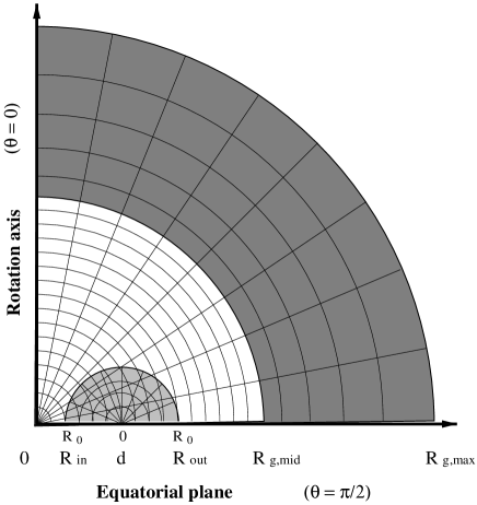
FIG. 1.: Schematic figure of the coordinate systems used in the actual computation. (a) A sketch of the coordinate systems for the star and the gravitational field. (b) The larger spherical coordinate system corresponds to that for gravitation (white and dark gray region). The smaller spherical coordinate system corresponds to that for the fluid (gray region). $R_{0}$ is defined as $R_{0}=(R_{\mathrm{o}ut}-R_{\mathrm{i}n})/2$.

Since we have assumed conformal flatness in space, we may introduce these spherical coordinate systems in the same manner as we do for Newtonian models. Especially, since the derivatives appearing in the basic equations are those for the flat 3-metric $f_{ij}$, it is convenient to take the non-coordinate basis whose metric becomes the unit matrix $f_{ij}=\delta_{ij}={\rm diag}(1,1,1)$ as is usually done for vector analysis in flat space, where $\delta_{ij}$ is the Kronecker delta. We write the orthonormal non-coordinate basis for the spherical coordinates as

$\displaystyle\{{\bf e}_{r},{\bf e}_{\theta},{\bf e}_{\varphi}\},\quad{\rm where}$

$${\bf e}_{a}\cdot{\bf e}_{b}=\delta_{ab},\quad(a,b=r,\theta,\varphi).$$ (75)

When necessary, we will distinguish the bases for the gravitational coordinate system and the fluid coordinate system by the superscripts $g$ and $f$, respectively. Using these bases, the gradient of a scalar function $\phi$ is written as

$$\nabla^{i}\phi=\nabla_{i}\phi={\bf e}_{r}\frac{\partial\phi}{\partial r}+{\bf e}_{\theta}\frac{1}{r}\frac{\partial\phi}{\partial\theta}+{\bf e}_{\varphi}\frac{1}{r\sin\theta}\frac{\partial\phi}{\partial\varphi}.$$ (76)

Hereafter, we often for convenience make use of the index notation and the notation of vector analysis in the same equation, as above.

B Poisson solver

Seven elliptic type PDEs appear in our formulation. They are Eqs. (21), (24), (27) and (28) for the gravitational field, and Eq. (65) for the fluid variable. To solve these equations, the flat part of 3D Laplacian is first separated out. Then, the equations are transformed into integral forms by using the Green’s function of the 3D Laplacian.

$$\Delta\phi_{(a)}=S_{(a)}.$$ (77)

Here the suffix $(a)$ is an index to specify each equation, and $\Delta$ is the 3D flat Laplacian in spherical coordinates,

$$\Delta\phi_{(a)}=\frac{1}{r^{2}}\frac{\partial}{\partial r}\left(r^{2}\frac{\partial\phi_{(a)}}{\partial r}\right)+$$ (79)

$$\frac{1}{r\sin\theta}\frac{\partial}{\partial\theta}\left(\sin\theta\frac{\partial\phi_{(a)}}{\partial\theta}\right)+\frac{1}{r^{2}\sin^{2}\theta}\frac{\partial^{2}\phi_{(a)}}{\partial\varphi^{2}}.$$

By using a Green’s function which satisfies the following equation

$$\Delta\left(-\frac{1}{4\pi}\frac{1}{\left|\bf{r}-\bf{r^{\prime}}\right|}\right)=\delta(\bf{r}-\bf{r^{\prime}}),$$ (80)

Eq. (77) is transformed as

$$\phi_{(a)}=-\frac{1}{4\pi}\int\frac{S_{(a)}}{\left|\bf{r}-\bf{r^{\prime}}\right|}dV^{\prime}+\chi,$$ (81)

where $\chi$ is either a function or a constant depending on the boundary condition. We use the Legendre expansion to compute the integral in Eq. (81),

$$\frac{1}{\left|\bf{r}-\bf{r^{\prime}}\right|}\,=\,\sum_{n=0}^{\infty}f_{n}(r,r^{\prime})\sum_{m=0}^{n}\epsilon_{m}\,\frac{(n-m)!}{(n+m)!}\,$$ (83)

$$\times P_{n}^{~{}m}(\cos\theta)\,P_{n}^{~{}m}(\cos\theta^{\prime})\cos m(\varphi-\varphi^{\prime}),$$

where $f_{n}(r,r^{\prime})$ is defined as,

$$f_{n}(r,r^{\prime})=\left\{\begin{array}[]{cc}\displaystyle\frac{1}{r}\left(\frac{r^{\prime}}{r}\right)^{n},\quad{\rm for}\quad r^{\prime}\leq r\ ,\\ \\ \displaystyle\frac{1}{r^{\prime}}\left(\frac{r}{r^{\prime}}\right)^{n},\quad{\rm for}\quad r\leq r^{\prime}\ ,\end{array}\right.$$ (84)

$\epsilon_{m}$ is defined as,

$$\epsilon_{m}=\left\{\begin{array}[]{ll}1\ ,\quad{\rm for}\quad m\,=\,0\ ,\\ \\ 2\ ,\quad{\rm for}\quad m\,=\,1,2,...,n,\end{array}\right.$$ (85)

and $P_{n}^{~{}m}(\cos\theta)$ is the associated Legendre function. Here $dV^{\prime}=r^{\prime 2}\sin\theta^{\prime}dr^{\prime}d\theta^{\prime}d\varphi^{\prime}$.

Eq. (81) is a formal solution in a sense that each source term $S_{(a)}$ also contains the variables $\{\phi_{(a)}\}$. Therefore, an iterative method is used to find a solution. All of the equations are consistently solved by a self-consistent-field (SCF) iteration scheme [20, 21, 22], whose procedure is described in detail in Paper I of [8].

C Solution method for the gravitational field

To apply the above procedure, we need to separate out the 3D flat Laplacian $\Delta$ for the spherical coordinates as in Eq. (79). We may regard $\nabla^{2}$ operating on scalar valued functions, as in Eqs. (21), (24) and (28), in the same way as $\Delta$ in Eq. (79). On the other hand, the Laplacian $\nabla^{2}$ operates on a vector valued function on the l.h.s. of Eq. (27). Although it is possible to use the Green’s function of the Laplacian for a vector valued function, instead, we explicitly write down its components and derive the form of Eq. (79) in each expression, so that we can follow the same procedure as for the scalars.

In the gravitational coordinates, this procedure goes as follows,

$$\nabla^{2}G^{j}=\nabla^{i}\nabla_{i}G^{j}=\Delta\left(G^{r}{\bf e}_{r}^{g}+G^{\theta}{\bf e}_{\theta}^{g}+G^{\varphi}{\bf e}_{\varphi}^{g}\right),$$ (86)

$$\left[\nabla^{2}G^{j}\right]^{r}={\bf e}_{r}\cdot\Delta\left(G^{r}{\bf e}_{r}^{g}+G^{\theta}{\bf e}_{\theta}^{g}+G^{\varphi}{\bf e}_{\varphi}^{g}\right)$$ (87)

$$=\Delta G^{r}-\frac{2}{r^{2}}\left(G^{r}+\frac{G^{\theta}}{\tan\theta}+\frac{1}{\sin\theta}\frac{\partial G^{\varphi}}{\partial\varphi}+\frac{\partial G^{\theta}}{\partial\theta}\right),$$ (88)

$$\left[\nabla^{2}G^{j}\right]^{\theta}={\bf e}_{\theta}\cdot\Delta\left(G^{r}{\bf e}_{r}^{g}+G^{\theta}{\bf e}_{\theta}^{g}+G^{\varphi}{\bf e}_{\varphi}^{g}\right)$$ (89)

$$=\Delta G^{\theta}-\frac{2}{r^{2}}\left(\frac{G^{\theta}}{2\sin^{2}\theta}+\frac{\cos\theta}{\sin^{2}\theta}\frac{\partial G^{\varphi}}{\partial\varphi}-\frac{\partial G^{r}}{\partial\theta}\right),$$ (90)

$$\left[\nabla^{2}G^{j}\right]^{\varphi}={\bf e}_{\varphi}\cdot\Delta\left(G^{r}{\bf e}_{r}^{g}+G^{\theta}{\bf e}_{\theta}^{g}+G^{\varphi}{\bf e}_{\varphi}^{g}\right)$$ (91)

$$=\Delta G^{\varphi}-\frac{2}{r^{2}}\left(\frac{G^{\varphi}}{2\sin^{2}\theta}-\frac{1}{\sin\theta}\frac{\partial G^{r}}{\partial\varphi}-\frac{\cos\theta}{\sin^{2}\theta}\frac{\partial G^{\theta}}{\partial\varphi}\right),$$ (92)

where Eqs. (87) $\sim$ (91) are the l.h.s. of Eq. (27). For the $\varphi$ component of Eq. (27), we multiply by $\sin\varphi$ and rearrange the terms of Eq. (91) as follows:

$$\sin\varphi\left[\nabla^{2}G^{j}\right]^{\varphi} = \sin\varphi\,{\bf e}_{\varphi}\cdot\Delta\left(G^{r}{\bf e}_{r}^{g}+G^{\theta}{\bf e}_{\theta}^{g}+G^{\varphi}{\bf e}_{\varphi}^{g}\right)$$ (93)

$$=\Delta(\sin\varphi\,G^{\varphi}) - \frac{2}{r^{2}\sin^{2}\theta}\left(-\sin\theta\sin\varphi\frac{\partial G^{r}}{\partial\varphi}\right.$$ (94)

$$- \left.\cos\theta\sin\varphi\frac{\partial G^{\theta}}{\partial\varphi}+\cos\varphi\frac{\partial G^{\varphi}}{\partial\varphi}\right).$$ (95)

In these expressions we suppress the subscript $g$ for the gravitational coordinates.

Terms appearing in expressions (87), (89) and (93) in addition to the flat 3D Laplacian $\Delta$ are transferred to the r.h.s. and are included as a part of the source term of each component. By the above rearrangement, all of the basic equations for the gravitational part have been written in the form of Eq. (77). Therefore, we can follow the procedure described in subsection III B. As we show in Table I, the boundary conditions are imposed by setting $\chi=1$ for Eqs. (21) and (24) and $\chi=0$ for Eqs. (27) and (28). Because of the symmetries for the variables shown in Table I, the source terms have corresponding symmetries as well. As a result, appropriate behaviors of integral terms in Eq. (81) at $r\rightarrow\infty$ are automatically satisfied.

D Solving method for the fluid part

The basic equations and boundary conditions for the fluid part are Eqs. (65) – (70). Since these equations are essentially the same as those of the Newtonian case solved in Paper I, we can apply all of the computational techniques developed in that paper. As we mentioned in subsection III A, we prepare the spherical coordinate system to compute the structure of the star whose origin is at the coordinate center of the star. The elliptic type PDE Eq. (65) is solved in this coordinate system by using the same procedure as in subsection III B. Eq. (65) has the same form as Eq. (77) and is integrated to give Eq. (81). To impose the boundary condition Eq. (68), we regard the term $\chi$ in Eq. (81) as a regular homogeneous solution of the Laplace equation inside the star, i.e.,

$$\Delta\chi(r_{f},\theta_{f},\varphi_{f})=0.$$ (96)

In the spherical coordinates, such a homogeneous solution to Eq. (96) can be expressed by using the associated Legendre functions as follows:

$$\chi(r_{f},\theta_{f},\varphi_{f})\,=\,\sum_{l=1}^{\infty}\sum_{m=1}^{l}\,a_{lm}\,r_{f}^{l}\,\left[1+(-1)^{l+m}\right]\,$$ (97)

$$\times\left(\frac{(2l+1)(l-m)!}{4\pi(l+m)!}\right)^{1/2}\,P_{l}^{~{}m}(\cos\theta_{f})\,\sin m\varphi_{f}\ ,$$ (98)

where $a_{lm}$’s are certain constants. Here we have taken into account the regularity of the solutions at $r_{f}=0$ and the symmetries listed in Table I. The coefficients $a_{lm}$ are computed so that the velocity potential $\Phi$ satisfies the boundary condition (68).

Eq. (67) is used to compute the density distribution within the star. For numerical computations, we introduce a function $q$ which is similar to the Emden function of Newtonian polytropes defined as follows:

$$q=\frac{P}{\rho}.$$ (99)

In terms of this function, we can express

$$\rho = \kappa^{-n}q^{n},$$ (100)

$$P = \kappa^{-n}q^{n+1},$$ (101)

$$h = 1+\left(n+1\right)q.$$ (102)

Substituting the last three expressions into Eq. (67), we find

$$q=\frac{1}{n+1}\left[\left(\frac{\lambda^{2}}{\alpha^{2}}-\Psi^{-4}\nabla_{i}\Phi\nabla^{i}\Phi\right)^{1/2}-1\right].$$ (103)

Accordingly, the matter source terms Eqs. (71)–(73) are rewritten as follows,

$$\rho_{H} = \kappa^{-n}q^{n}\left(\frac{\lambda^{2}}{\left(1+\left(n+1\right)q\right)\alpha^{2}}-q\right),$$ (104)

$$\rho_{H} + 2S\,=\,\kappa^{-n}q^{n}$$ (105)

$$\times \left(\frac{3\lambda^{2}}{\left(1+\left(n+1\right)q\right)\alpha^{2}}-\left(2+\left(2n-3\right)q\right)\right),$$ (106)

$$j^{i} = \kappa^{-n}q^{n}\frac{\lambda}{\left(1+\left(n+1\right)q\right)\alpha}\Psi^{-4}\nabla^{i}\Phi.$$ (107)

For the numerical computation of the fluid part, it is convenient to introduce the surface fitted spherical coordinate system as used in the Newtonian case [8]. The surface of one NS in the binary system can be expressed by a function $R_{S}(\theta_{f},\varphi_{f})$ even when the deformation of the shape is relatively large. By using this function, the new coordinates $(r_{f}^{*},\theta_{f}^{*},\varphi_{f}^{*})$ are defined as follows,

$$r_{f}^{*}=\frac{r_{f}}{R_{S}(\theta_{f},\varphi_{f})},\quad\theta_{f}^{*}=\theta_{f},\quad{\rm and}\quad\varphi_{f}^{*}=\varphi_{f}.$$ (108)

The stellar interior with the assumed symmetry is mapped into the region $(r_{f}^{*},\theta_{f}^{*},\varphi_{f}^{*})\in[0,1]\times[0,\pi/2]\times[0,\pi]$. The surface fitted coordinate is advantageous for computing numerical derivatives and imposing boundary conditions at the stellar surface. Implementation of this coordinate system is described in detail in Paper I.

E Normalization of quantities and choice of parameters

Non-dimensionalization of variables and proper choices of parameters are important for the iteration scheme to obtain converged equilibrium configurations stably. For convenience in making numerical computations, we rescale the coordinate length so that the coordinate radius of the star at the intersection of the surface and the coordinate line with $(\theta_{g},\varphi_{g})=(\pi/2,0)$ is unity, namely, we introduce a parameter $R_{0}$ so that $R_{S}(\pi/2,0)/R_{0}=1=R_{S}(\pi/2,\pi)/R_{0}$ in the fluid coordinates.

By using this $R_{0}$, the basic equations for the gravitational potentials, Eqs. (21), (24), (27) and (28), whose forms are essentially the same as Eq. (77) or Eq. (81), become as follows,

$$\widehat{\Delta}\phi_{(a)}=\widehat{S}^{~{}g}_{(a)}+\kappa^{-n}R_{0}^{~{}2}\,\widehat{S}^{~{}m}_{(a)},$$ (109)

$$\phi_{(a)}=\chi-\frac{1}{4\pi}\int\frac{\widehat{S}_{(a)}^{~{}g}+\kappa^{-n}R_{0}^{~{}2}\,\widehat{S}_{(a)}^{~{}m}}{\left|\widehat{\bf{r}}\,-\,\widehat{\bf{r}}^{\prime}\right|}d\widehat{V}^{\prime},$$ (110)

where $\widehat{\Delta}=R_{0}^{~{}2}\,\Delta$. Here $\widehat{S}^{~{}m}_{(a)}$ stands for the non-dimensionalized part of the matter source terms corresponding to Eqs. (71)–(73) or (104)–(107) and $\widehat{S}^{~{}g}_{(a)}$ denotes remaining terms. We explicitly show the dependence of these quantities on the parameters $\kappa$ and $R_{0}$. In the equations for the fluid part, $\kappa$ and $R_{0}$ are canceled out after rescaling and non-dimensionalization. By this rescaling, the coordinates and variables are transformed as follows,

$$\widehat{r}=\frac{r}{R_{0}},\quad\widehat{\nabla}_{i}=R_{0}\nabla_{i},\quad\widehat{\xi}^{i}=\frac{\xi^{i}}{R_{0}},\quad\widehat{R}_{S}=\frac{R_{S}}{R_{0}},$$ (111)

$$\widehat{K}_{ij}=\widetilde{K}_{ij}R_{0},\quad\widehat{B}=\frac{B}{R_{0}},\quad\widehat{\Phi}=\frac{\Phi}{R_{0}},\quad\widehat{\Omega}=\Omega R_{0}.$$ (112)

We may consider that $\kappa$ is used for non - dimensionalization of the variables, and $R_{0}$ for rescaling of the numerical computations. However, since these two parameters appear in the equations only through the following combination:

$$\bar{R}_{0}=\kappa^{-n/2}R_{0},$$ (113)

we can regard them as a single parameter when we compute each solution. In this paper, we only consider $\kappa={\rm const}$ sequences, which could be appropriate for investigation of the final inspiraling stage of BNS’s. (When constructing solutions, we could mimic physical effects such as heating by changing the value of $\kappa$.)

We then have three parameters $\bar{R}_{0}$, $\widehat{\Omega}$ and $C$ in the basic equations. We need to impose three more conditions to specify them. For this purpose, we choose three locations where $q$ has definite values. Namely, we set $q=0$ at the intersections of the surface and the coordinate line with $(\theta_{g},\varphi_{g})=(\pi/2,0)$, i.e. at the two points $(r_{f}^{*},\theta_{f}^{*},\varphi_{f}^{*})=(1,\pi/2,0)$ and $(1,\pi/2,\pi)$ and also set $q=q_{c}$ at a grid point where $q$ takes the largest value inside the star [23] . Since we have introduced the surface $\widehat{R}_{S}(\theta_{f}^{*},\varphi_{f}^{*})$ in the surface fitted coordinates, the former two conditions are explicitly imposed by setting $\widehat{R}_{S}(\pi/2,0)=1=\widehat{R}_{S}(\pi/2,\pi)$.

The above three conditions are applied to Eq. (67) at three points to get equations for $\bar{R}_{0}$, $\widehat{\Omega}$ and $C$. It is known [21, 10] that $\alpha$ and $\Psi$ are scaled as

$$\alpha=\widehat{\alpha}^{\bar{R}_{0}^{2}},\qquad\Psi=\widehat{\Psi}^{-\bar{R}_{0}^{2}/2}.$$ (114)

By using this rescaling, Eq. (67) is written as,

$$\widehat{\alpha}^{2\bar{R}_{0}^{2}}\left\{1+\left(n+1\right)q\right\}^{2}+\left(\widehat{\alpha}\widehat{\Psi}\right)^{2\bar{R}_{0}^{2}}\widehat{\nabla}_{i}\widehat{\Phi}\,\widehat{\nabla}^{i}\widehat{\Phi}$$ (115)

$$-\left\{C+\left(\widehat{\Omega}\,\widehat{\xi}^{i}-\omega^{i}\right)\widehat{\nabla}_{i}\widehat{\Phi}\right\}^{2}=0.$$ (116)

We use three equations which are derived by imposing the above three conditions at three points in the star, namely, at the inner and outer edges and at the coordinate center of the star. These three non-linear algebraic equations with respect to $\bar{R}_{0}$, $\widehat{\Omega}$ and $C$ are solved by using the Newton-Raphson method and their values are updated through the iteration procedure.

The above choice is known to make the iteration converge stably. This choice of parameters and the computation scheme for them are essentially the same as those for rotating single stars [21] or those for co-rotating BNS’s [10] in GR.

F Discretization and numerical computation

Since we have rescaled the length by $R_{0}$, the computational domain is measured by this unit. For the gravitational coordinate system, the whole computational domain is taken as $(\widehat{r}_{g},\theta_{g},\varphi_{g})\in[0,\widehat{R}_{g,\rm max}]\times[0,\pi/2]\times[0,\pi/2]$. It is discretized equidistantly for the $\theta_{g}$ and $\varphi_{g}$ directions. For the $\widehat{r}_{g}$ direction, we divide the region into two parts as $[0,\widehat{R}_{g,\rm mid}]$ (the white region in Figure 1(b)) and $[\widehat{R}_{g,\rm mid},\widehat{R}_{g,\rm max}]$ (the dark gray region in Figure 1(b)). We discretize the region $[0,\widehat{R}_{g,\rm mid}]$ equidistantly, and the region $[\widehat{R}_{g,\rm mid},\widehat{R}_{g,\rm max}]$ non-equidistantly. By denoting grid points as $(\widehat{r}_{i},\theta_{j},\varphi_{k})$, in which we suppress the subscript $g$, the discretization becomes as follows,

$$\widehat{r}_{i+1}-\widehat{r}_{i} = \frac{\widehat{R}_{g,\rm mid}}{N^{r}_{g,\rm mid}},\quad{\rm where}\quad$$ (117)

$$0 \leq \widehat{r}_{j}\leq\widehat{R}_{g,\rm mid},\ \left(0\leq j\leq{N^{r}_{g,\rm mid}}\right),$$ (118)

$$\widehat{r}_{i+1}-\widehat{r}_{i} = \delta(\widehat{r}_{i}-\widehat{r}_{i-1}),\quad{\rm where}\quad$$ (119)

$$\widehat{R}_{g,\rm mid} \leq \widehat{r}_{j}\leq\widehat{R}_{g,\rm max},\ \left({N^{r}_{g,\rm mid}}\leq j\leq{N^{r}_{g,\rm max}}\right),$$ (120)

$$\theta_{i+1}-\theta_{i} = \frac{\pi/2}{N^{\theta}_{g}},\quad{\rm where}\quad$$ (121)

$$0 \leq \theta_{j}\leq\frac{\pi}{2},\ \left(0\leq j\leq{N^{\theta}_{g}}\right),$$ (122)

$$\varphi_{i+1}-\varphi_{i} = \frac{\pi/2}{N^{\varphi}_{g}},\quad{\rm where}\quad$$ (123)

$$0 \leq \varphi_{j}\leq\frac{\pi}{2},\ \left(0\leq j\leq{N^{\varphi}_{g}}\right).$$ (124)

In Eq. (120), $\delta(>1)$ is a certain constant.

The surface fitted fluid coordinate system is discretized equidistantly in all directions as follows,

$$r^{*}_{i+1}-r^{*}_{i} = \frac{1}{N^{r}_{f}},\quad{\rm where}\quad$$ (125)

$$0 \leq \widehat{r}^{*}_{j}\leq 1,\ \left(0\leq j\leq{N^{r}_{f}}\right)$$ (126)

$$\theta^{*}_{i+1}-\theta^{*}_{i} = \frac{\pi/2}{N^{\theta}_{f}},\quad{\rm where}\quad$$ (127)

$$0 \leq \theta^{*}_{j}\leq\frac{\pi}{2},\ \left(0\leq j\leq{N^{\theta}_{f}}\right),$$ (128)

$$\varphi^{*}_{i+1}-\varphi^{*}_{i} = \frac{\pi}{N^{\varphi}_{f}},\quad{\rm where}\quad$$ (129)

$$0 \leq \varphi^{*}_{j}\leq\pi,\ \left(0\leq j\leq{N^{\varphi}_{f}}\right).$$ (130)

The fluid coordinate system is always set within the region $[0,R_{g,\rm mid}]$ of the gravitational coordinate system in order to maintain an accuracy. Standard finite differences are applied for the basic equations with these grid points, which maintain at least second order accuracy.

In the present computation, we typically took the values listed in Table II. A finer mesh is used for the region $[0,\widehat{R}_{g,\rm mid}]$ whose size in the $\widehat{r}_{g}$ direction is about 2.5 times the diameter of one NS for the cases with types S, M, and L and 2 times for the case with type Ls. The region $[\widehat{R}_{g,\rm mid},\widehat{R}_{g,\rm max}]$ is discretized into $20$ grid points in the $\widehat{r}_{g}$ direction. Types S, M, and L are mainly used to show the convergence of the scheme as functions of the mesh size and we will mention this in a later section. The mesh sizes of type S and type M in the region $0\leq\widehat{r_{g}}\leq\widehat{R}_{g,\rm mid}$ are, respectively, $1/2$ and $3/4$ of that of the finest type L. Type Ls is used for compute the configurations for rather small separations, although the numerical results of type L and type Ls are almost the same.

$\widehat{R}_{g,\rm mid}$	$\widehat{R}_{g,\rm max}$	$N^{r}_{g,\rm mid}$	$N^{r}_{g,\rm max}$	$N^{\theta}_{g}$	$N^{\varphi}_{g}$	$N^{r}_{f}$	$N^{\theta}_{f}$	$N^{\varphi}_{f}$	type
$5$	$100$	$40$	$20$	$20$	$30$	$8$	$8$	$16$	S
$5$	$100$	$60$	$20$	$30$	$45$	$12$	$12$	$24$	M
$5$	$100$	$80$	$20$	$40$	$60$	$16$	$16$	$32$	L
$4$	$100$	$80$	$20$	$40$	$40$	$20$	$40$	$28$	Ls

TABLE II.: Parameters for the computational domains and the numbers of grid points in each coordinate system are listed.

Strictly speaking, $\widehat{R}_{g,\rm max}$ should be infinite in order to impose asymptotically flatness as a boundary condition. This could be implemented by using a certain appropriate coordinate transformation to compactify an infinite region, which has been used by several authors [24, 25]. Although this is straightforward, we do not implement such a special treatment for simplification in the present numerical code. Instead, we truncate the computational domain at large $\widehat{R}_{g,\rm max}$. It is known that such truncation does not affect the local properties of the space-time or the structure of each NS [26]. Although the choice of the value of $R_{g,max}$ would affect the values of the physical quantities very little, it would be safer to cover the space as extensively as possible. We take a rather large value for $\widehat{R}_{g,\rm max}=100$ as shown in Table II. Because of this choice, the error introduced into an integral quantity such as the ADM mass by this truncation (see Eq. (137) below) does not affect the digits of the numerical results presented in the later sections.

We also truncate the order of the Legendre expansion in Eq. (83) and Eq. (97) at finite values instead of infinity. We denote the maximum value of the expansion for quantities in the gravitational coordinates in Eq. (83) as $n_{\rm max}$ and that for the fluid coordinates in Eq. (83) and Eq. (97) (i.e. the expansion for the velocity potential) as $l_{\rm max}$. Typically, we use $(n_{\rm max},l_{\rm max})=(32,12)$. Therefore sources of truncation error are the finite difference and the truncation for this expansion. The results depend very little on $l_{\rm max}$ when we choose $l_{\rm max}>8$. We will show how the results depend on $n_{\rm max}$ in a later section.

As was mentioned before, the basic equations are solved iteratively. The iteration procedure is the same as that for Newtonian irrotational BNS models described in Paper I. The only difference in the numerical scheme is that an interpolation of physical quantities from one coordinate system to the other is required. We implemented the cubic spline interpolation method for all directions of the coordinates. As we will show in the later sections, one of the interesting problems relating to the irrotational binary sequence is to determine the behavior of the maximum density as the binary stars approach. To investigate this problem, it is quite important to compute a smooth density distribution. In fact, an interpolation scheme of 1st order accuracy does not give a smooth density distribution, especially around the central region. Therefore, we have employed the cubic spline interpolation which keeps smoothness of interpolated data, although the cost for numerical computations is rather large.

In our formulation, each quasi-equilibrium configuration is specified by three parameters, namely, the half of the separation between the coordinate centers of the two component stars $\widehat{d}$, the largest value of $q_{c}$ on the discretized grid, and the polytropic index $n$. (Note that $\kappa$ has been scaled out.) The initial guess for the numerical iteration may be, for instance, an analytic solution of a Newtonian spherical polytrope with $n=1$ at larger separation, say $\widehat{d}=2$. We have started the iteration by setting $q_{c}$ to be a small value and could then follow iteration cycles. We have regarded the obtained solution as being a converged one when relative differences of physical variables of subsequent iterations on each coordinate grid point are less than a certain small value, typically we choose $10^{-5}$. Once we get a converged solution, we can change the values of parameters by a few tenths of a percent. Typically, a solution is converged after 100 $\sim$ 300 iteration cycles. It takes about $1$ minute for one iteration cycle using a DEC Alpha-station 1/166.

IV Numerical results for irrotational binary systems in GR

A Integrals

In this section we show several integral quantities of the equilibrium configurations. The total rest-mass energy $M_{0,\rm tot}$ of the two component stars is defined as

$$M_{0,\rm tot}=\int_{\cal M}\rho u^{\mu}d\Sigma_{\mu}=\int_{\cal M}\rho u^{\mu}\left(-n_{\mu}\sqrt{\gamma}\right)dV,$$ (131)

where ${\cal M}$ denotes the integration region which is the support of the two component stars. The non-dimensional form of the total rest-mass can be written using Eq. (111) and (113) as

$$\bar{M}_{0,\rm tot}=\kappa^{-n/2}M_{0,\rm tot} = \kappa^{-n/2}{R}_{0}^{3}\int_{\cal M}\kappa^{-n}q^{n}\frac{\lambda}{h\alpha}\Psi^{6}d\widehat{V}$$ (132)

$$= \bar{R}_{0}^{3}\int_{\cal M}\frac{q^{n}\lambda\Psi^{6}}{h\alpha}d\widehat{V}.$$ (133)

where $d\widehat{V}=dV/R_{0}^{3}$. The total mass-energy (ADM mass) is

$$M_{\rm ADM} = -\frac{1}{2\pi}\oint_{\infty}\nabla^{i}\Psi d^{2}S_{i}=-\frac{1}{2\pi}\int_{\infty}\nabla^{2}\Psi dV,$$ (134)

$$= \frac{1}{16\pi}\int_{\infty}\Psi^{-7}\widetilde{K}_{ij}\widetilde{K}^{ij}dV+\int_{\cal M}\Psi^{5}\rho_{H}\,dV$$ (135)

where Eq. (21) derived from the Hamiltonian constraint is used. This can be rewritten in the non-dimensional form as,

$$\bar{M}_{\rm ADM} = \kappa^{-n/2}M_{\rm ADM}=\frac{\bar{R}_{0}}{16\pi}\int_{\infty}\Psi^{-7}\widehat{K}_{ij}\widehat{K}^{ij}d\widehat{V}$$ (137)

$$+\bar{R}_{0}^{3}\int_{\cal M}\Psi^{5}q^{n}\left(\frac{\lambda^{2}}{h\alpha^{2}}-q\right)d\widehat{V}.$$

The angular momentum is aligned with the $\theta_{g}=0$ axis and can be defined as (see, e.g., [27])

$$J_{\rm tot} = \frac{1}{8\pi}\oint_{\infty}f_{ij}\xi^{i}\widetilde{K}^{jk}d^{2}S_{k}=\frac{1}{8\pi}\int_{\infty}f_{ij}\xi^{i}\nabla_{k}\widetilde{K}^{jk}dV$$ (138)

$$= \int_{\cal M}\Psi^{10}f_{ij}\xi^{i}j^{j}dV=\int_{\cal M}\Psi^{10}r_{g}\sin\theta_{g}j^{\varphi}\,dV,$$ (139)

where we used $\nabla_{k}\widetilde{K}^{jk}=\Psi^{10}D_{k}K^{jk}$ as well as the momentum constraints (6), and $\xi=r_{g}\sin\theta_{g}{\bf e}_{\varphi}^{g}$ from the definition. This is the total angular momentum contained in the space-time including both the orbital and spin angular momentum of the stars. Finally, we can substitute Eq. (107) for $j^{i}$ and write the angular momentum in the non-dimensional form

$$\bar{J}_{\rm tot} = \kappa^{-n}J_{\rm tot}=\bar{R}_{0}^{4}\int_{\cal M}\Psi^{10}\widehat{r}_{g}\sin\theta_{g}\widehat{j}^{\varphi}\,d\widehat{V}$$ (140)

$$= \bar{R}_{0}^{4}\int_{\cal M}\Psi^{6}\widehat{r}_{g}\sin\theta_{g}\frac{q^{n}\lambda}{h\alpha}\widehat{\nabla}^{\varphi}\Phi\,d\widehat{V}.$$ (141)

In the following we will denote a half of the total rest-mass, the ADM mass and the angular momentum by $\bar{M}_{0}=\bar{M}_{0,\rm tot}/2$, $\bar{M}=\bar{M}_{\rm ADM}/2$ and $\bar{J}=\bar{J}_{\rm tot}/2$, respectively. In the limit of large separation, $\bar{M}_{0}$ and $\bar{M}$ approach the corresponding values for isolated stars.

We also use the averaged separation $d_{G}$ which coincides with the separation between mass centers of the two component stars in Newtonian limit, namely,

$$\bar{d}_{G} = \kappa^{-n/2}d_{G}$$ (142)

$$= \frac{\bar{R}_{0}}{\bar{M}_{0}}\int_{\cal M}\widehat{r}_{g}\sin\theta_{g}\cos\varphi_{g}\frac{q^{n}\lambda\Psi^{6}}{h\alpha}d\widehat{V}.$$ (143)

B Test of our new computational method

In this paper we will show results for $n=1$ polytropes. For this we need to specify two parameters in order to obtain one quasi-equilibrium configuration, i.e. the half of separation $\widehat{d}$ and the largest value of $q=q_{c}$. In order to check how our new computational code works, we have compared our results with (a) those of co-rotating GR binary systems tabulated in [10], and (b) those of the Newtonian irrotational binary systems in Paper I. With the former comparison (a), we can check the gravitational field part of our code for the strong gravity regime. We have also performed (c) a convergence test for the Newtonian case since it is desirable to show how the scheme actually converges to some analytic or semi-analytic results.

Concerning irrotational binary systems, Taniguchi [28] has analytically solved semi-detached irrotational binary systems with the 1PN approximation for $n=0$ polytropes and Taniguchi and Nakamura recently developed a method to treat the compressible Newtonian case [29]. Lombardi, Rasio & Shapiro have calculated the irrotational polytropic binary systems by partly including 1PN correction terms [30]. It will be important to perform the convergence test with these results as well as making a comparison with numerical results obtained by other authors who have used the identical formulation but different numerical computational methods.

It is convenient to characterize solutions or sequences by using the total rest mass $M_{0}={\rm const}$ or, equivalently, the compactness $(M/R)_{\infty}$ of an isolated spherical star. In actual computations, we choose a certain value for $M_{0}$ and adjust the parameter $q_{c}$ during the iteration so that the value of $M_{0}$ is kept constant.

1 Comparison with other works

Below, we show the results of comparison tests (a) and (b). In this section, type Ls in Table II is used for the numerical grids. For the expansions in Eq. (83) and Eq. (97), we include terms up to $(n_{\rm max},l_{\rm max})=(20,12)$.

In Table III, we compare our results for co-rotating binary systems with those in [10]. For these models we have replaced the equations for the fluid part by those for co-rotating fluids. Therefore, the code for the gravitational part has been checked. We set the values of $\widehat{d}$ and $q_{c}$ to be the same as those in [10] for each model. As shown in Table III, the calculated quantities $\bar{\Omega}$ and $\bar{R}_{0}$ which characterize the models for BNS’s are in good agreement (relative differences are less than $1\%$). For the integral quantities $\bar{M}_{0}$, $\bar{M}$ and $\bar{J}$, the relative differences are at most $2\%$.

$z_{A}$	$\widehat{d}$	$q_{c}$	$\bar{\Omega}$	$\bar{R}_{0}$	$\bar{M}_{0}$	$\bar{M}$	$\bar{J}$
0.20	1.50	0.0685	0.079	1.004	0.1118	0.10552	0.02729
			0.079	1.005	0.1125	0.10619	0.02780
0.00	1.00	0.0658	0.101	1.177	0.1118	0.10551	0.02715
			0.101	1.176	0.1128	0.10637	0.02760
0.20	1.50	0.2450	0.168	0.646	0.1781	0.16013	0.04948
			0.168	0.643	0.1801	0.16169	0.05050
0.00	1.00	0.2164	0.202	0.780	0.1781	0.16018	0.05024
			0.203	0.774	0.1807	0.16227	0.05132

TABLE III.: Comparison between the results of Baumgarte et al. (1997) and those obtained with the present method for co-rotating GR binary systems. The first line of each model corresponds to the results of Baumgarte et al. (1997) and the second line to the present results. The first two models correspond to the system with $(M/R)_{\infty}=0.1$ and the latter two models to $(M/R)_{\infty}=0.2$ in Baumgarte et al. (1997). $z_{A}=0.0$ corresponds to a contact binary system and $z_{A}=0.2$ to a semi-detached binary system where $z_{A}=R_{\mathrm{i}n}/R_{\mathrm{o}ut}$.

Next, we compare our results for a quasi-equilibrium sequence of irrotational binary systems in weak gravity with those of Newtonian computations. It is reasonable to assume that the total rest mass is constant throughout the final evolution. Thus the quasi-equilibrium sequence with $M_{0}={\rm const}$ mimics the realistic evolution sequence as a result of GW emission. In Figure 2, we compare our present results for the compactness $(M/R)_{\infty}=0.001$ with those in Paper I. In this figure, $\bar{J}$ is plotted against the separation $\bar{d}_{G}$ or $\bar{\Omega}$. Relative differences of $\bar{J}$ at a fixed value of $\bar{d}_{G}$ or $\bar{\Omega}$ are $\sim 0.5\%$, relative differences of $\bar{d}_{G}$ at a fixed value of $\bar{J}$ are $\sim 1\%$, and relative differences of $\bar{\Omega}$ at a fixed value of $\bar{J}$ are $\sim 1.7\%$. Therefore, our new code has reproduced the same results as those of other computations with reasonable accuracy.

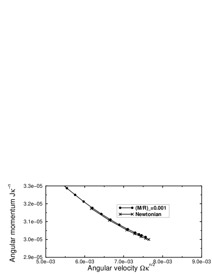
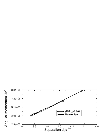
FIG. 2.: Comparison between the results of Paper I (Newtonian) and those of the present computation (with compactness $(M/R)_{\infty}=0.001$). Quasi-equilibrium sequences for irrotational BNS systems with weak gravity (curve with dots) and with Newtonian gravity (curve with crosses) are plotted. The angular momentum as a function of the angular velocity (upper panel) and the angular momentum as a function of the separation (lower panel) are shown.

2 Convergence test

In order to see how well our numerical solutions approximate true solutions, we have estimated the influence of the mesh size on the results. This can be done by investigating how the values of physical quantities behave when the mesh size is varied. For this convergence test, we have used types S, M, and L in Table II for numerical computations. We chose $(n_{\rm max},l_{\rm max})=(20,12)$ for the expansions. In Fig. 3, we plot the relative differences of the angular momentum $J$ and the angular velocity $\Omega$ from those of the semi-analytic results of the ellipsoidal approximation [31] for types S, M and L with values of the separation $d/R_{0}$ being fixed. The plots clearly show that for global quantities, our results tend to converge as the mesh size is decreased. Note that even for $d/R_{0}=2.0$, the difference between the polar radius and the equatorial radius is $\sim 3\%$ and this means that the results of the ellipsoidal approximation are reasonably accurate.

On the other hand we need to be more careful about the convergence of local quantities such as the density distribution, the shape of the star, or the metric potential distribution. Since we will discuss dependence of the maximum density on the binary separation in a later section, we here discuss the property of the convergence of the maximum density as a representative of local quantities.

In Fig. 4(a), we plot the maximum rest mass density $\rho_{\rm max}$ against the half separation $d/R_{0}$, normalized by the $R_{0}$ of each model, to show the convergence of solutions as the mesh type is changed. In the figure, the curves correspond to the mesh type S (the line with crosses), the mesh type M (the line with diamonds), and the mesh type L (the line with filled circles), respectively. We again set $(n_{\rm max},l_{\rm max})=(20,12)$. The maximum density $\rho_{\rm max}(d/R_{0})$ does not change monotonically as the separation changes, and does not tend exactly to the asymptotic value $\rho_{\rm max,\infty}$, which is the central density of an isolated spherical star computed from the TOV equation. However, the curves oscillate around $\rho_{\rm max,\infty}$ and the differences from it are at most $1\%$ even for the smallest mesh type S. Note that the resolution of the star in the gravity coordinates becomes coarser for larger separations. For instance, the mesh number of the gravity coordinates which cover the neutron star radius is only $6$ points in the $\varphi_{g}$ coordinate at $d/R_{0}\sim 3.0$ for the mesh type S.

To show that $\rho_{\rm max}(d/R_{0})$ converges to a certain number for each separation, we plot the relative difference of $\rho_{\rm max}$, $\Delta\rho_{\rm max}/\rho_{\rm ex}$ against the mesh size, in Fig. 4(b). Here the relative difference is measured in terms of the value $\rho_{\rm ex}$ extrapolated from the values obtained for the mesh types S, M and L in Table II for each $d/R_{0}$. This figure shows that the local quantities such as the density also converge as the number of mesh points is increased.

The relative difference of the maximum density is roughly proportional to $(\Delta r)^{2}$ around $d/R_{0}\sim 1.5$. This is satisfactory since we are interested in configurations with $d/R_{0}<2.0$, since the deformation of a star is small even at $d/R_{0}=2.0$. For example the difference between the major and minor radii is only a few $\%$. Therefore, analytic or semi-analytic approximations could be applied to configurations down to this separation [28, 29, 30]. The results also indicate that the truncation error of the expansion $n_{\rm max}$ is negligible for the case with $d/R_{0}\mathrel{\raise 1.29167pt\hbox{$<$}\mkern-14.0mu\lower 2.58334pt\hbox{$\sim$}}1.5$ when we choose $n_{\rm max}\mathrel{\raise 1.29167pt\hbox{$>$}\mkern-14.0mu\lower 2.58334pt\hbox{$\sim$}}20$.

To clarify the very small non-monotonic behavior of $\rho_{\rm max}(d/R_{0})$, we have computed sequences with $M/R=0.001$ by changing the number of the Legendre functions in the expansion for the gravitational potential, $n_{\rm max}$, in Eq. (83). In Figure 5(a), we plot $\rho_{\rm max}(d/R_{0})$ for $n_{\rm max}=16$, $20$ and $24$, using the mesh type M. For $n_{\rm max}=16$, the relative difference from the asymptotic value becomes $\mathrel{\raise 1.29167pt\hbox{$<$}\mkern-14.0mu\lower 2.58334pt\hbox{$\sim$}}1.5\%$ at larger separations $d/R_{0}\mathrel{\raise 1.29167pt\hbox{$>$}\mkern-14.0mu\lower 2.58334pt\hbox{$\sim$}}2.5$. On the other hand, the differences between the $n_{\rm max}=20$ and $n_{\rm max}=24$ configurations are less than $0.5\%$ everywhere and $\rho_{\rm max}(d/R_{0})$ at larger separation almost reaches the asymptotic value $\rho_{\rm max,\infty}$. From this figure we may conclude that the number of the Legendre functions in the expansion, $n_{\rm max}$, should be larger than 20. We also note that there arises a restriction for $n_{\rm max}$ and $l_{\rm max}$ from the number of grid points, since the number of numerical grid points should be enough to resolve the periodic behavior as well as the orthogonality of the Legendre functions and trigonometric functions used in Eq. (83) and Eq. (97). In Figure 5(b), we plot $\rho_{\rm max}(d/R_{0})$ for the $n_{\rm max}=20$ and $32$ sequences computed by using the mesh type L. The result with $n_{\rm max}=32$ shows that the density is almost constant for $1.8\mathrel{\raise 1.29167pt\hbox{$<$}\mkern-14.0mu\lower 2.58334pt\hbox{$\sim$}}d/R_{0}\mathrel{\raise 1.29167pt\hbox{$<$}\mkern-14.0mu\lower 2.58334pt\hbox{$\sim$}}2.2$. We stress again that the present numerical computation is targeted to compute highly deformed configurations of component stars with $d/R_{0}\mathrel{\raise 1.29167pt\hbox{$<$}\mkern-14.0mu\lower 2.58334pt\hbox{$\sim$}}2.0$. Since all of the curves behave almost similarly for $d/R_{0}\mathrel{\raise 1.29167pt\hbox{$<$}\mkern-14.0mu\lower 2.58334pt\hbox{$\sim$}}2.0$, our computations are accurate enough to discuss the increase or decrease of $\rho_{\rm max}(d/R_{0})$ of the solution sequence. Therefore a reasonable choice is $n_{\rm max}\mathrel{\raise 1.29167pt\hbox{$>$}\mkern-14.0mu\lower 2.58334pt\hbox{$\sim$}}20$. It should be noted that the integrated physical quantities depend little on the number $n_{\rm max}$ if $n_{\rm max}\mathrel{\raise 1.29167pt\hbox{$>$}\mkern-14.0mu\lower 2.58334pt\hbox{$\sim$}}20$.

Concerning the $l_{\rm max}$, that is the number of terms in the expansion for the velocity potential $\Phi$, this does not affect local or global quantities when we choose $l_{\rm max}>8$. For instance, the choice of grid type L and $l_{\rm max}=12$ is enough to compute $\Phi$ accurately at any separation.

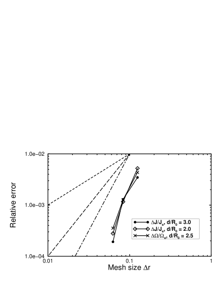
FIG. 3.: Results of the convergence test for the weak gravity configurations (compactness $(M/R)_{\infty}=0.001$). Relative differences between the present results and those of the semi-analytic calculations with the ellipsoidal approximation by Lai, Rasio and Shapiro (1994) are plotted. The points on each line correspond to the results for the mesh types S, M and L in Table II. We plot the mesh size of the r-direction on the horizontal axis. The short dashed line is proportional to $\Delta r$, the long dashed line to $(\Delta r)^{2}$, and the dash dotted line to $(\Delta r)^{3}$.

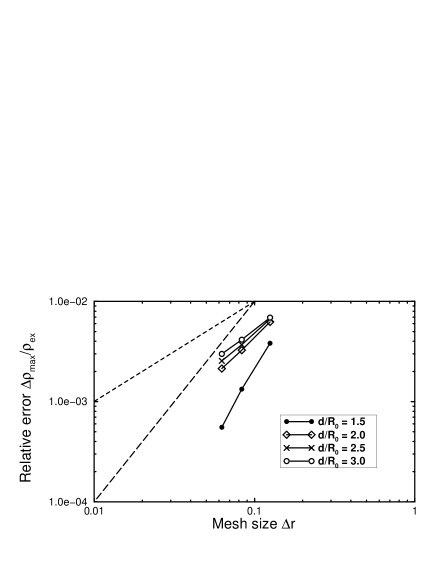
FIG. 4.: The convergence test for the maximum rest mass density $\rho_{\rm max}$ for the case with compactness $(M/R)_{\infty}=0.001$. (a) $\rho_{\rm max}(d/R_{0})$ is plotted. Each line corresponds to a different mesh size, the mesh type S (the line with crosses), the mesh type M (the line with diamonds), and the mesh type L (the line with filled circles), respectively. The long dashed line shows $\rho_{\rm max}$ of an isolated spherical star $\rho_{\rm max,\infty}$. The short dashed lines show $\pm 0.5\%$ difference from this value. (b) The convergence of the relative error for $\rho_{\rm max}$. The mesh size of the r-direction is used for the horizontal axis to represent the resolution. The short dashed line is proportional to $\Delta r$ and the long dashed line to $(\Delta r)^{2}$.

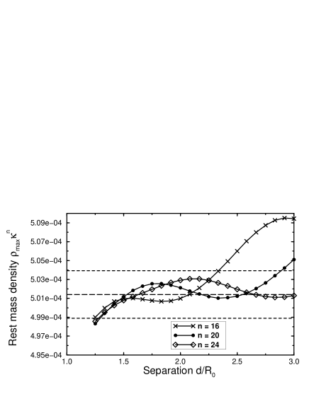
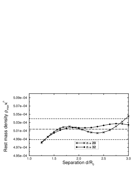
FIG. 5.: The dependence of $\rho_{\rm max}(d/R_{0})$ on the order of Legendre expansion of the gravitational potential $n_{\rm max}$ for the case with $(M/R)_{\infty}=0.001$. Each line corresponds to a different value of $n_{\rm max}$. (a) The mesh type M is used for computations. (b) The mesh type L is used for computations. The horizontal long dashed line shows the $\rho_{\rm max}$ of an isolated spherical star $\rho_{\rm max,\infty}$. The horizontal short dashed lines show $\pm 0.5\%$ difference from this value.

C Quasi-equilibrium sequences of irrotational binary systems in GR

In Figures 6 and 7 we show contours for GR irrotational BNS systems. We have used mesh types L and Ls for the computations in this subsection. As seen from these figures, our numerical method can handle highly deformed configurations of BNS systems and the gravitational field around them. In particular, in the right panel of Fig. 6, we show the contours for the rest mass density $\rho$ with $(M/R)_{\infty}=0.14$. From this figure, we can see that a cusp-like structure appears at the inner edge of stars before the two stars make contact with each other [33]. The cusp is supposed to correspond to the inner Lagrange point (L1 point), with mass overflow occurring from this point when the separation of two stars becomes smaller enough.

FIG. 6.: Contours of the conformal factor $\Psi^{4}$ (upper left panel), the rest mass density distribution (upper right panel) and the shift vector with the stellar surfaces (lower right panel), for the model with $(M/R)_{\infty}=0.14$ and $\widehat{d}=1.25$ in $XY$-plane ($\theta_{g}=\theta_{f}=\pi/2$-plane). Lengths in the figures are normalized with $R_{0}$.

FIG. 7.: Structure of a component star of an irrotational BNS system. Contours of the distribution of rest mass density $\rho$ (upper three panels) and of the velocity potential $\Phi$ (lower three panels) are drawn for the model with $(M/R)_{\infty}=0.17$ and $\widehat{d}=1.25$. $YZ$-plane (upper left panel), $ZX$-plane (upper right) and $XY$-plane (lower right panel) correspond to the $\varphi_{f}=0$ and $\pi$ plane, the $\varphi_{f}=\pi/2$ plane, and the $\theta_{f}=\pi/2$ plane, respectively. Lengths in the figures are normalized with $R_{0}$.

In Table IV, we tabulate the values of physical quantities for irrotational BNS systems with a cusp-like structure for various degrees of compactness. We also plot the dimensionless total angular momentum $J_{\rm tot}/M_{\rm ADM}^{2}$ in Fig. 8 which is unity for an extreme Kerr black hole. For the co-rotating models [10], $J_{\rm tot}/M_{\rm ADM}^{2}$ becomes unity around $(M/R)_{\infty}\sim 0.175$. On the other hand, this value for irrotational BNS systems becomes unity around $(M/R)_{\infty}\sim 0.12$ as shown in Table IV. Since there exists a velocity field which rotates in the counter direction with respect to the orbital motion of each component star, the total angular momentum becomes smaller. Therefore, after coalescence of the two stars due to GW emission, irrotational BNS systems could form a single Kerr black hole by losing much less angular momentum from the system than co-rotating BNS systems.

$(M/R)_{\infty}$	$\bar{M}_{0}$	$\bar{M}$	$\Omega M_{0}$	$J_{\rm tot}/M_{\rm ADM}^{2}$	$\bar{R}_{0}$
0.1	0.112	0.105	0.0110	1.08	1.07
0.12	0.130	0.121	0.0148	1.01	0.979
0.14	0.146	0.135	0.0192	0.963	0.899
0.17	0.166	0.150	0.0271	0.911	0.783

TABLE IV.: Physical quantities of the irrotational BNS near to the configuration with a cusp-like structure (L1 point).

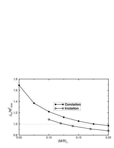
FIG. 8.: Comparison of $J_{\rm tot}/M_{\rm ADM}^{2}$ between co-rotational and irrotational BNS systems at the closest distances for various values of the compactness parameter $(M/R)_{\infty}$. For the co-rotating models, values for the contact phases are plotted. For the irrotational models, those for the configurations with cusps are displayed.

In Figures 9, we show quasi-equilibrium sequences for several values of $(M/R)_{\infty}$. The binding energy $(M-M_{\infty})/M_{\infty}$ and $\bar{J}$ are plotted against the normalized orbital angular velocity $\Omega M_{0}$. Since each curve is a sequence with constant rest mass $M_{0}$, an evolutionary track of a BNS system as a result of GW emission can be approximated by following each curve from smaller to larger values of $\Omega M_{0}$. The terminal points of the curves, i.e. the points with the largest $\Omega M_{0}$, roughly correspond to configurations with an L1 point. In analogy with Newtonian models as well as with GR co-rotating binary systems [10, 34], turning points on these curves are expected to correspond to the points where dynamical instability sets in. Our results show that none of the systems with different values of the compactness $(M/R)_{\infty}$ have turning points. Therefore irrotational binary configurations with $n=1$ are thought to be dynamically stable. In other words, at the final inspiraling phase, it is probable that the mass exchange starts earlier than the onset of the orbital motion instability.

FIG. 9.: The binding energy (upper panel) and the angular momentum (lower panel) are plotted against the orbital angular velocity. Each curve corresponds to an $M_{0}={\rm const}$ sequence. The value of the compactness $(M/R)_{\infty}$ of an isolated star is attached to each curve. Cusp-like shape appears for the terminal model with the largest $\Omega M_{0}$ along each curve.

D Individual collapse of the irrotational BNS system

There are two main reasons why the close binary system of irrotational stars has attracted wide attention. One is that, as mentioned in Section I, it is more probable that such a situation is realized just before coalescence due to GW emission, since viscosity is not strong enough to synchronize the spin of a NS and the orbital motion [3] at this stage. The other reason is that the numerical simulation of irrotational binary systems done by Wilson, Mathews and Marronetti [9] showed the result that the maximum density of each NS increases during the inspiraling due to the GR effect. They proposed a new scenario for the final inspiraling phase of irrotational BNS systems, namely, each component star of a BNS system individually collapses to form a binary black hole system, and after that two black holes would coalesce.

This scenario has been debated by many authors (see [15, 35] and references therein). Recent numerical computations by Marronetti, Mathews and Wilson [16] again show the maximum density increasing by a few percent for a sequence of models with larger compaction $(M/R)_{\infty}=0.19$, although the most recent re-computations by Mathews and Wilson give a much smaller central density increase for polytropes [36]. On the other hand, the computation by the Meudon numerical relativity group [15] does not show this tendency. In Figure 10, we show our results for the relative change of the maximum energy density $(e_{\rm max}-e_{\infty})/e_{\infty}$ of a star against the separation $\widehat{d}$. Here $e=\rho(1+\varepsilon)$, $e_{\rm max}$ is its maximum value and $e_{\infty}$ is its value in an isolated state which is computed by solving the TOV equation.

We show the results for $n_{\rm max}=20$ in Fig. 10(a) and $n_{\rm max}=32$ in Fig. 10(b). We notice that the results do not depend on the order of the Legendre expansion $n_{\rm max}$ for $d/R_{0}\mathrel{\raise 1.29167pt\hbox{$<$}\mkern-14.0mu\lower 2.58334pt\hbox{$\sim$}}2.0$ with any values of the compactness. For $d/R_{0}\mathrel{\raise 1.29167pt\hbox{$>$}\mkern-14.0mu\lower 2.58334pt\hbox{$\sim$}}2.0$, $e_{\rm max}$ does not become constant for $n_{\rm max}=20$ but tends to being almost constant when we choose $n_{\rm max}=32$. To show the convergence around $d/R_{0}\mathrel{\raise 1.29167pt\hbox{$<$}\mkern-14.0mu\lower 2.58334pt\hbox{$\sim$}}2.0$ clearly, differences between the result with $n_{\rm max}=32$ and $n_{\rm max}=20$, $(e_{\rm max,\,32}-e_{\rm max,\,20})/e_{\infty}$, are plotted in Fig. 10(c). The relative difference $(e_{\rm max,\,32}-e_{\rm max,\,20})/e_{\infty}$ is less than $0.35\%$ at $d/R_{0}\leq 2.0$ for all $(M/R)_{\infty}\leq 0.19$.

Differences of the relative change of the central density $(e_{\rm max}-e_{\infty})/e_{\infty}$ at larger separation $d/R_{0}\mathrel{\raise 1.29167pt\hbox{$>$}\mkern-14.0mu\lower 2.58334pt\hbox{$\sim$}}2.0$ get larger as the compactness becomes larger. For instance they are $0.5\%$ and $1\%$ for $(M/R)_{\infty}=0.17$ and $0.19$, respectively. However, in any case, differences are $\mathrel{\raise 1.29167pt\hbox{$<$}\mkern-14.0mu\lower 2.58334pt\hbox{$\sim$}}1\%$ for any value of the compactness as shown in Fig. 10(b) and $e_{\rm max}$ tends to a constant value when the component stars are detached. Therefore we may discuss the change of $(e_{\rm max}-e_{\infty})/e_{\infty}$ along each solution sequence. Our results show that the energy density changes in the range of $0.5\%$ to $2.5\%$ and decreases as the separation decreases. Therefore, we do not observe the maximum density to increase and hence there is no tendency towards individual collapse in the present computation. Also the rate of decrease of the maximum energy density around $d/R_{0}\mathrel{\raise 1.29167pt\hbox{$<$}\mkern-14.0mu\lower 2.58334pt\hbox{$\sim$}}2.0$ is larger for larger $(M/R)_{\infty}$.

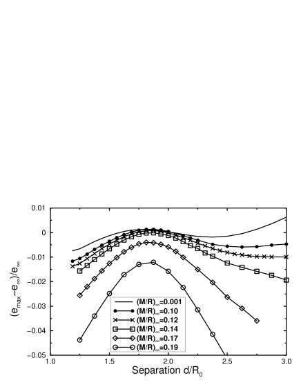
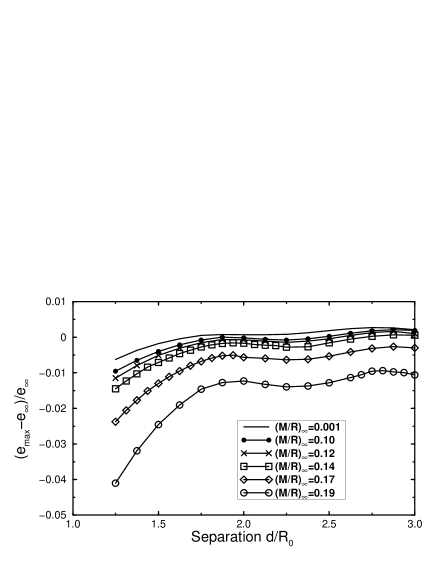
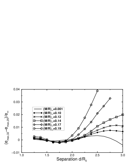
FIG. 10.: The relative change of the maximum energy density is plotted against the separation. The horizontal axis corresponds to the coordinate separation in units of $R_{0}$ for each model. (a) The results computed setting the order of expansion to $n_{\rm max}=20$. Curves are plotted for $(M/R)_{\infty}=0.001$ to $0.19$. (b) The results computed setting the order of expansion to $n_{\rm max}=32$. Curves are plotted for $(M/R)_{\infty}=0.001$ to $0.19$. The maximum density does not increase as the separation decreases. (c) The differences between the results with $n_{\rm max}=32$ and $n_{\rm max}=20$. Curves are plotted for $(M/R)_{\infty}=0.001$ to $0.19$. These two results converge for $d/R_{0}\mathrel{\raise 1.29167pt\hbox{$<$}\mkern-14.0mu\lower 2.58334pt\hbox{$\sim$}}2.0$.

V Discussion and conclusion

A Position of the present numerical method

As mentioned in section II A, there are two different numerical schemes for solving irrotational binary star systems in GR [15, 16]. The basic formulation and basic equations are almost the same but the numerical schemes are different.

Bonazzola, Gourgoulhon and Marck [15] have used the multi-domain pseudo spectral method. They have introduced several coordinate systems one of which is a coordinate system fitted to the stellar surface. The basic equations which are essentially the same as those in this paper are solved by using the pseudo-spectral method on each of these domains. Although the implementation of this numerical method is rather complicated, it produces numerically ‘exact’ solutions with excellent accuracy.

Marronetti, Mathews and Wilson [16] have used a Cartesian coordinate system and a finite difference method. The equations which they solved are also the same as ours except for their approximate treatment on the boundary condition for the velocity potential equation [37]. Although their computation is rather less accurate, Cartesian coordinates are commonly used in 3D numerical relativity to compute dynamical coalescence of compact binary systems, and hence it could be advantageous for providing initial data for future 3D simulations of BNS coalescence.

Despite the existence of these two methods, we have presented another scheme in this paper. There are several reasons for this. Firstly, since quasi-equilibrium states of binary neutron star systems have an important significance in GW investigations, it would be better to get reliable solutions by studying them from many directions even if this is the same problem. Secondly, results obtained from the two previous schemes seem to be somewhat different. In particular, the behavior of the maximum density during the evolution is different as discussed in subsection IV D, although the recent re-computation by Mathews and Wilson [36] gives consistent results with others for the polytropic configurations.

In our solution method, we have used the integral form to solve Poisson type equations. A spherical coordinate system is introduced to implement this Poisson solver. From our experience with numerical computations, it seems desirable to use spherical coordinate systems to solve for the structures of component stars. On the other hand, to solve for the gravitational field, it is possible to implement Cartesian coordinates and suitable sophisticated Poisson solvers for the coordinates (for instance, the multi-grid method, ICCG, and so on). In our scheme, the coordinates for the star are patched on those for the gravitational field. This can be applied straightforwardly for a Cartesian grid. Such an implementation could also be useful for preparing initial conditions for numerical simulations as well as for checking the present numerical results.

B Future prospects

It is important to compute quasi-equilibrium configurations to connect the inspiraling phase, where the perturbative expansion technique can be applied, to the merging phase, where fully dynamical computations are required. Such computations are also useful since the quasi-equilibrium solutions give accurate and appropriate initial conditions for simulations of BNS coalescence [6]. Recently, a simulation of coalescing irrotational BNS systems in 3D full general relativity has been performed using the solutions of the present paper as initial configurations [17]. The successful result of these simulations may be considered as showing that the present results are reliable for use as initial data for binary coalescence.

In our formulation we have used the so called Wilson–Mathews formulation to treat the GR effects. However it is known that this approach is exact only up to 1PN order for binary systems in terms of the post-Newtonian terminology, although 2PN or higher order corrections should be included to express realistic BNS systems. Asada and Shibata [14] have formulated the Einstein equations so as to express BNS systems exactly up to 2PN order. Implementing their equations in numerical computations may be one of the possible ways to construct quasi-equilibrium BNS systems, although it is necessary to solve 29 elliptic PDEs simultaneously for the gravitational field. Recently, Usui, Uryū and Eriguchi [38] have developed a new scheme to compute quasi-equilibrium configurations by using a quite different form of the metric from that of the Wilson–Mathews formulation. It would be interesting to compare results from that method with our present results. Also several authors have constructed a formulation for so called ‘intermediate binary black hole’ (IBBH) states [39]. This formulation could also be applicable to quasi-equilibrium states of BNS systems.

C Summary and conclusion

We have constructed a numerical method to compute quasi-equilibrium states of irrotational binary systems composed of compressible gaseous stars in general relativity. The new numerical method is based on a standard finite difference method and therefore implementation is rather simple and straightforward. We have used two coordinate systems for the computation, one for the gravitational field variables and the other for the fluid variables. Physical quantities are interpolated from one to the other. We have shown that such a procedure works well by actual numerical computations of irrotational BNS systems in GR.

The basic equation for the irrotational flow becomes an elliptic PDE with a Neumann type boundary condition at the stellar surface. For the treatment of general relativistic gravity, we have used the Wilson–Mathews formulation. In this formulation, the basic equations are again expressed by a system of elliptic PDEs. We have developed a method to solve these PDEs. We have calibrated our solutions by using the results of independent numerical computations as well as of semi-analytic calculations. We have also tested the convergence of these numerical solutions.

We have succeeded in computing quasi-equilibrium sequences of irrotational BNS systems in GR. As in the Newtonian case, the BNS systems have been found to be dynamically stable during the inspiraling stage until Roche lobe overflow starts at the L1 point. The quasi-equilibrium sequences also suggest that no substantial increase of the maximum energy density occurs during the inspiraling phase as a result of GW emission. Further investigations of numerical computations and implementation of various realistic EOS’s and/or a realistic formulation of GR gravity are interesting and inevitable issues for theoretical predictions of GW signals supposed to be detected by the interferometric GW detectors in the next century.

- [1] A. Abramovici et al., Science 256, 325 (1992); C. Bradaschia et al., Nucl. Instrum. and Methods A289, 518 (1990); J. Hough, in Proceedings of the Sixth Marcel Grossmann Meeting, edited by H. Sato and T. Nakamura (World Scientific, Singapore, 1992), p.192; K. Kuroda et al., in Proceedings of the international conference on gravitational waves: Sources and Detectors, edited by I. Ciufolini and F. Fidecard (World Scientific, Singapore, 1997), p.100.
- [2] Edited by T. Nakamura, Perturbative and Numerical Approaches to Gravitational Waves, Prog. Theor. Phys. Suppl., 128, (1997) ; F. A. Rasio and S. L. Shapiro, Class. Quant. Grav., in press, (gr-qc/9902019).
- [3] C. S. Kochanek, ApJ 398, 234 (1992); L. Bildsten and C. Cutler, ApJ 400, 175 (1992).
- [4] K. Oohara and T. Nakamura, in Relativistic gravitation and gravitational radiation, edited by J.-P. Lasota and J.-A. Marck (Cambridge University Press, Cambridge, 199), 309; T. Nakamura and K. Oohara, in Numerical Astrophysics, edited by S. Miyama (1998) (gr-qc/9812054).
- [5] E. Seidel and W. M. Suen, submitted to J. Comput. Appl. Math., (1999).
- [6] M. Shibata, Prog. Theor. Phys. 101, 251 (1999); M. Shibata, Prog. Theor. Phys. 101, 1199 (1999); M. Shibata, PRD, in press (1999) (gr-qc/9908027).
- [7] S. L. Shapiro and S. A. Teukolsky, Black Holes, White Dwarfs and Neutron Stars, (Wiley, New York, 1983).
- [8] K. Uryū and Y. Eriguchi, MNRAS 296, L1 (1998a), (astro-ph/9712203); K. Uryū and Y. Eriguchi, ApJS 118, 563 (1998b) Paper I, (astro-ph/9808118); K. Uryū and Y. Eriguchi, MNRAS 303, 329 (1999), (astro-ph/9808120); K. Uryū and Y. Eriguchi, to be published in the proceedings of 19th Texas Symposium on Relativistic Astrophysics: Texas in Paris, Paris, France (1998).
- [9] J. R. Wilson and G. J. Mathews, Phys. Rev. Lett. 75, 4161 (1995); J. R. Wilson, G. A. Mathews and P. Marronetti, Phys. Rev. D54, 1317 (1996).
- [10] T. W. Baumgarte, G. B. Cook, M. A. Scheel, S. L. Shapiro and S. A. Teukolsky, Phys. Rev. D57, 7299 (1998).
- [11] M. Shibata, Phys. Rev. D58, 024012 (1998).
- [12] S. A. Teukolsky, ApJ 504, 442 (1998).
- [13] S. Bonazzola, E. Gourgoulhon and J.-A. Marck, Phys. Rev. D56, 7740 (1997); H. Asada, Phys. Rev. D57, 7292 (1998).
- [14] H. Asada and M. Shibata, Phys. Rev. D54, 4944 (1996); M. Shibata, Phys. Rev. D55, 6019 (1997).
- [15] S. Bonazzola, E. Gourgoulhon and J.-A. Marck, to be published in the proceedings of 19th Texas Symposium on Relativistic Astrophysics: Texas in Paris, Paris, France (1998); S. Bonazzola, E. Gourgoulhon and J.-A. Marck, Phys. Rev. Lett. 82, 892 (1999).
- [16] P. Marronetti, G. J. Mathews and J. R. Wilson, to be published in the proceedings of 19th Texas Symposium on Relativistic Astrophysics: Texas in Paris, Paris, France (1998); P. Marronetti, G. J. Mathews and J. R. Wilson, to be published in Phys. Rev. D (1999).
- [17] M. Shibata, K. Uryū, Phys. Rev. D, in press (1999).
- [18] M. Shibata and T. Nakamura, Phys. Rev. D52, 5428 (1995).
- [19] A. H. Taub, Arch. Ratl. Mech. Anal. 3, 312 (1959); B. Carter, in Active Galactic Nuclei, edited by C. Hazard and S. Mitton (Cambridge University Press, Cambridge, 1979), p.273; V. Moncrief, ApJ 235, 1038 (1980).
- [20] I. Hachisu, ApJS 62, 461 (1986).
- [21] H. Komatsu, Y. Eriguchi, I. Hachisu, MNRAS 237, 355 (1989).
- [22] J. P. Ostriker, J. W.-K. Mark, ApJ 151, 1075 (1968).
- [23] Instead of this choice, we also set at the coordinate center of the star, that is , in some cases. The results do not change with this different choice.
- [24] G. B. Cook, S. L. Shapiro and S. A. Teukolsky, ApJ 398, 203 (1992).
- [25] S. Bonazzola, E. Gourgoulhon and J.-A. Marck, Phys. Rev. D58, 104020 (1998).
- [26] T. Nozawa, N. Stergioulas, E. Gourgoulhon, Y. Eriguchi, A&AS 132, 431 (1998).
- [27] J. M. Bowen and J. W. York, Jr., Phys. Rev. D21, 2047 (1980).
- [28] K. Taniguchi, Prog. Theor. Phys. 101, 283 (1999); K. Taniguchi, PhD thesis, Kyoto University, (1999).
- [29] K. Taniguchi and T. Nakamura, Phys. Rev. Lett., in press, (1999).
- [30] J. C. Lombardi, Jr., F. A. Rasio and S. L. Shapiro, Phys. Rev. D56, 3416 (1997).
- [31] D. Lai, F. A. Rasio and S. L. Shapiro, ApJ 420, 811 (1994).
- [32] We also approximate a function in Eq. (97) with a finite order of expansion . However this truncation does not affect this artificial behavior for the change of . In fact, we did not observe this behavior in the purely Newtonian calculation [8], in which we used the same truncation for but a different scheme to compute the Newtonian gravitational potential.
- [33] The cusp is formed before the two stars make contact with each other even for Newtonian equal mass BNS’s with polytropic EOS, because of the non-synchronized rotation of the stars. This fact was overlooked in the previous paper by the present authors (Paper I). Although the cusp forms just before the contact phase, changes of numerical results are of less than and the statements in [8] are not affected. The authors thank Dr. E. Gourgoulhon for pointing this out.
- [34] D. Lai, F. A. Rasio and S. L. Shapiro, ApJS 88, 205 (1993); T. W. Baumgarte, G. B. Cook, M. A. Scheel, S. L. Shapiro and S. A. Teukolsky, Phys. Rev. D57, 6181 (1998).
- [35] P. Marronetti, G. J. Mathews and J. R. Wilson, Phys.Rev. D58, 043003 (1998).
- [36] G. J. Mathews and J. R. Wilson, submitted to Phys. Rev. D (1999), (gr-qc/9911047).
- [37] We have implemented the approximate treatment on the boundary condition for the velocity potential equation used by [16]. The result of was the same as the exact treatment in this paper for but solutions did not converge for highly deformed configurations with , for the case with .
- [38] F. Usui, K. Uryū and Y. Eriguchi, Phys. Rev. D, Phys. Rev. D61, 024039 (1999).
- [39] P. R. Brady, J. D.E. Creighton and K. S. Thorne, Phys. Rev. D58, 061501 (1998); K. S. Thorne, submitted to Phys. Rev. D (1998), (gr-qc/9808024).