Continuous Self-Similarity Breaking in Critical Collapse

Abstract

This paper studies near-critical evolution of the spherically symmetric scalar field configurations close to the continuously self-similar solution. Using analytic perturbative methods, it is shown that a generic growing perturbation departs from the Roberts solution in a universal way. We argue that in the course of its evolution, initial continuous self-similarity of the background is broken into discrete self-similarity with echoing period $\Delta=\sqrt{2}\pi=4.44$, reproducing the symmetries of the critical Choptuik solution.

I Introduction

Critical phenomena in gravitational collapse have been a relatively recent and interesting development in the established field of general relativity. Following the numerical work of Choptuik on the spherically symmetric collapse of the minimally coupled massless scalar field [1], critical behavior was discovered in most common matter models encountered in general relativity, including pure gravity [2], null fluid [3] and, more generally, perfect fluid [4, 5], as well as more exotic models.

The essence of critical phenomena in general relativity is the fact that just at the threshold of black hole formation, the dynamics of the field evolution becomes relatively simple and, in some important aspects, universal, despite the complicated and highly non-linear form of the equations of motion. In analogy with second order transitions in condensed matter physics, the mass of the black hole produced in near-critical gravitational collapse scales as a power law

$$M_{\text{BH}}(p)\propto|p-p^{*}|^{\beta},$$ (1)

with parameter $p$ describing initial data, and the mass-scaling exponent $\beta$ is dependent only on the matter model, but not on the initial data family. The critical solution, separating solutions with black hole formed in the collapse from the ones without a black hole, also depends on the matter model only, and serves as an intermediate attractor in the phase space of solutions. It often has an additional symmetry called self-similarity, in either continuous or discrete flavors.

Discovery of critical phenomena in gravitational collapse was the first real success of numerical relativity in which a physical effect was observed in simulations without being first predicted by theoretical physicists. For the theoretician, the challenge and attraction of studying critical phenomena lies in the possibility of exploring a new class of exact solutions of Einstein’s equations, having simple properties and high symmetry, but previously undiscussed. Another interesting thing about critical solutions is that they are very relevant to the cosmic censorship conjecture, the long-unsolved problem of general relativity. With their ability to produce arbitrarily small black holes and, in the critical limit, curvature singularity without an event horizon, in the course of quite generic gravitational collapse, they may serve as an acceptable counterexample to the cosmic censorship conjecture (see [7] and references therein).

Universality of the near-critical behavior has been explained by perturbation analysis and renormalization group ideas [3, 4, 5, 6], and is rooted in the fact that critical solutions generally have only one unstable perturbation mode. In the course of evolution of the near-critical initial field configuration, all the perturbations modes contained in it decay, forgetting details of the initial data and bringing the solution closer to critical, except the single growing mode which will eventually drive the solution to black hole formation or dispersal. In this sense, the critical solution acts as an intermediate attractor in the phase space of all field configurations. Because there is only single growing mode, the codimension of the attractor is one. The eigenvalue of the growing mode determines how rapidly the solutions will eventually depart from critical, and it can be used to calculate the mass-scaling exponent $\beta$.

As we have mentioned, the critical solution often has additional symmetry besides the usual spherical symmetry, called continuous or discrete self-similarity. This symmetry essentially amounts to the solution being independent of (in case of continuous self-similarity) or periodic in (in case of discrete self-similarity) one of the coordinates, a scale. The role of this symmetry in critical collapse is not understood at all. Some attempts at finding critical solutions made a continuously self-similar ansatz and hit a jackpot [3], whereas others studied discretely self-similar solutions from phenomenological point of view [8]. Yet the simple question of why a particular matter model should have this or that version of self-similarity incorporated in the critical solution still remains a mystery.

This paper attempts to shed some light on the subject by investigating the dynamics of formation of discretely self-similar structure in the gravitational collapse of a minimally coupled massless scalar field. As a base point of our investigation, we consider a certain continuously self-similar solution, known as the Roberts solution, as a toy-model of the critical solution in the gravitational collapse of a scalar field. This solution was constructed as a counterexample to the cosmic censorship conjecture [9] and was later rediscovered in the context of critical gravitational collapse [10, 11]. While not a proper attractor [12], this simple solution resembles in some of its properties more complicated critical solutions known only numerically. The aim of the present work is to show how, at least in the linear approximation, the discretely self-similar structure arises dynamically in the scalar field collapse. The advantage of our approach is that, due to the simple form of the Roberts solution, calculations can be carried out analytically and so provide additional independent insights different from numerical treatments.

Using linear perturbation analysis and Green’s function techniques, we study evolution of the spherically symmetric scalar field configurations close to the continuously self-similar solution. Approximating late-time evolution via the method of stationary phase, we find that a generic growing perturbation departs from the Roberts solution in a universal way. In the course of the evolution, initial continuous self-similarity of the background is broken into discrete self-similarity by the growing perturbation mode, reproducing the symmetries of the Choptuik solution. We are able to calculate the echoing period of the formed discretely self-similar structure analytically, and its value is close to the result of numerical simulations.

II The Roberts Solution

The starting point of our investigation is the Roberts solution, which will serve as a background for linear perturbation analysis. It is a solution describing gravitational collapse of a minimally coupled massless scalar field, described by the Einstein-scalar field equations

$$R_{\mu\nu} = 2\phi_{,\mu}\phi_{,\nu},$$ (2)

$$\Box\phi = 0,$$ (3)

which is spherically symmetric and also continuously self-similar. The latter symmetry means that there exists a vector field $\xi$ such that

$${\pounds}_{\xi}g_{\mu\nu}=2g_{\mu\nu},\hskip 10.00002pt{\pounds}_{\xi}\phi=0,$$ (4)

where ${\pounds}$ denotes the Lie derivative. Under these assumptions the field equations can be solved analytically, which is most easily done in null coordinates [10, 11, 13]. Self-similar solutions form a one-parameter family. As the parameter is varied, spacetimes both with and without a black hole occur. The solution just at the threshold of black hole formation is given by the metric

$$ds^{2}=-2\,du\,dv+r^{2}\,d\Omega^{2},$$ (5)

where

$$r=\sqrt{u^{2}-uv},\hskip 10.00002pt\phi=\frac{1}{2}\ln\left[1-\frac{v}{u}\right].$$ (6)

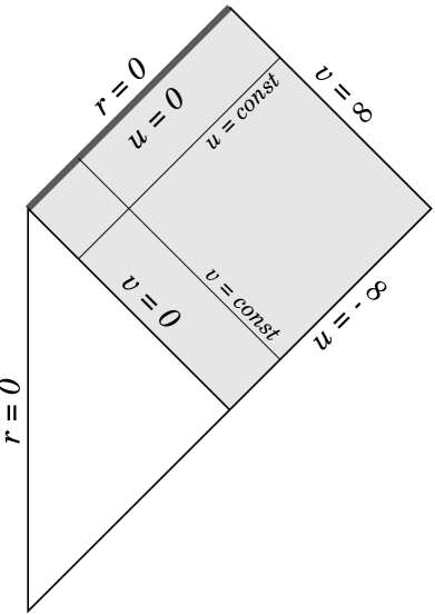
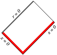
The global structure of the corresponding spacetime is shown in Fig. 1. The influx of the scalar field is turned on at the advanced time $v=0$, so that the Roberts spacetime is smoothly matched to Minkowskian flat spacetime to the past of this surface. The junction conditions, required for continuity of the solution there, serve as boundary conditions for the field equations (2) and (3). More detailed discussion of this important point is provided in Appendix A.

The evolution of perturbations of the Roberts solution is most easily followed in a coordinate system exploiting scale-invariance of the background, so that the self-similarity becomes apparent. Therefore, we introduce new coordinates, which we will call scaling coordinates, by

$$x=\frac{1}{2}\ln\left[1-\frac{v}{u}\right],\hskip 10.00002pts=-\ln(-u),$$ (7)

with the inverse transformation

$$u=-e^{-s},\hskip 10.00002ptv=e^{-s}(e^{2x}-1).$$ (8)

The signs are chosen to make the arguments of the logarithm positive in the region of interest ($v>0$, $u<0$), where the field evolution occurs. In these coordinates the metric (5) becomes

$$g_{\mu\nu}\,dx^{\mu}dx^{\nu}=2e^{2(x-s)}\left[(1-e^{-2x})ds^{2}-2dsdx\right]+r^{2}\,d\Omega^{2},$$ (9)

and the Roberts solution (6) is simply

$$r=e^{x-s},\hskip 10.00002pt\phi=x.$$ (10)

Observe that the scalar field $\phi$ does not depend on the scale variable $s$ at all, and the only dependence of the metric coefficients on the scale is through the conformal factor $e^{-2s}$. This is a direct expression of the geometric requirement (4) in scaling coordinates; the homothetic Killing vector $\xi$ is simply $-\frac{\partial\ }{\partial s}$.

III Gauge-Invariant Perturbations of the Roberts Solution

Since we are ultimately concerned with the dynamics of the breaking of the fields away from the Roberts solution, the effect due to the growing perturbation modes, we will only consider spherically symmetric perturbations here. Non-spherically symmetric perturbations decay [14] and so do not play a role in the critical behavior. In this section, we outline how spherically symmetric perturbations of the Roberts solution (5) are described in gauge-invariant formalism. A general spherically-symmetric metric perturbation is

$$\delta g_{\mu\nu}dx^{\mu}dx^{\nu}=k_{uu}\,du^{2}+2k_{uv}\,du\,dv+k_{vv}\,dv^{2}+r^{2}K\,d\Omega^{2},$$ (11)

while general perturbation of the scalar field is

$$\delta\phi=\varphi.$$ (12)

Under a (spherically-symmetric) gauge transformation generated by the vector

$$\xi^{\mu}=(A,B,0,0),$$ (13)

the metric and scalar field perturbations transform as

$$\Delta g_{\mu\nu}={\pounds}_{\xi}g_{\mu\nu},\hskip 10.00002pt\Delta\phi={\pounds}_{\xi}\phi.$$ (14)

The explicit expressions for the change in the perturbation amplitudes under the gauge transformation generated by the vector $\xi$ are

$$\Delta k_{uu} = -2B_{,u},$$ (15)

$$\Delta k_{uv} = -A_{,u}-B_{,v},$$ (16)

$$\Delta k_{vv} = -2A_{,v},$$ (17)

$$r^{2}\Delta K = (2u-v)A-uB,$$ (18)

$$2r^{2}\Delta\varphi = vA-uB.$$ (19)

Out of four metric and one matter perturbation amplitudes one can build the total of three gauge-invariant quantities, one describing matter perturbations

$$f=\frac{K}{2}-\varphi+\frac{1}{2u}\int k_{vv}\,dv,$$ (20)

and the other two describing metric perturbations

$$\rho=(r^{2}K)_{,uv}+k_{vv}-k_{uv}-uk_{uu,v}/2+(2u-v)k_{vv,u}/2,$$ (21)

$$\sigma=k_{uv}-\frac{1}{2}\int k_{vv,u}\,dv-\frac{1}{2}\int k_{uu,v}\,du.$$ (22)

The linearized Einstein-scalar field equations

$$\delta R_{\mu\nu}=4\phi_{(,\mu}\delta\phi_{,\nu)},\hskip 10.00002pt\delta(\Box\phi)=0$$ (23)

can then be rewritten completely in terms of these gauge-invariant quantities. It is possible to show that the field equations reduce to one master differential equation for the scalar field perturbation,

$$2u(u-v)f_{,uv}+(2u-v)f_{,v}-uf_{,u}-2f=0,$$ (24)

and two trivial equations relating metric perturbations to the scalar field perturbation

$$\sigma_{,u}=2f_{,u}+2f/u,\hskip 10.00002pt\rho=0.$$ (25)

Once the gauge-invariant quantities are identified, one is free to switch between various gauges. We conclude this section by discussing two particularly convenient choices.

Field gauge ($K=k_{vv}=0$): The scalar field perturbation coincides with the gauge-invariant quantity $f$ in this gauge, and expressions for other gauge-invariant quantities simplify considerably:

$$f = -\varphi,$$ (26)

$$\rho = -k_{uv}-uk_{uu,v}/2,$$ (27)

$$\sigma = k_{uv}-\frac{1}{2}\int k_{uu,v}\,du.$$ (28)

The linearized Einstein-scalar field equations are at their simplest in this gauge, and the derivation of the master equation for $f$ above is almost transparent. The metric and scalar field perturbation amplitudes are trivial to obtain:

$$\varphi = -f,$$ (29)

$$k_{uv} = 2f,$$ (30)

$$k_{uu,v} = -4f/u.$$ (31)

Null gauge ($k_{uu}=k_{vv}=0$): This gauge was used in the original analysis of spherically-symmetric perturbations of the Roberts solution [12]. The motivation behind this gauge choice is that coordinates $u$ and $v$ remain null in the perturbed spacetime. The expressions for gauge-invariant quantities are quite simple here as well:

$$f = K/2-\varphi,$$ (32)

$$\rho = (r^{2}K)_{,uv}-k_{uv},$$ (33)

$$\sigma = k_{uv}.$$ (34)

For details on how to reconstruct perturbation amplitudes from gauge-invariant quantities see [12].

IV Wave Propagation on the Roberts Background

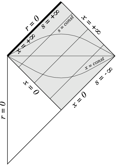
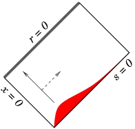
So, we wish to study scalar field wave propagation on the Roberts background. Typically, one would specify initial data for the wavepacket either on some spacelike Cauchy surface or on initial null surface, and trace the later evolution using the field equations. Our choice for initial surface is $u=\text{const}$ ($s=0$), which forms a complete null surface if extended to the center of the flat spacetime part, as illustrated in Fig. 2. The part of a pulse propagating through flat background evolves trivially, and can be equivalently replaced by specifying field values on $v=0$ hypersurface. Thus, in our problem, the initial conditions for the linearized Einstein-scalar field equations are given on the $s=0$ surface, while the boundary conditions are determined by junction conditions across the null shell $v=0$, as outlined in Appendix A, and the requirement that the perturbations be bounded at future infinity.

As was shown earlier, the Einstein-scalar field equations for the spherically symmetric perturbations of the Roberts solution can be reduced to the master differential equation

$${\cal D}f(x,s)=0$$ (35)

for the single gauge-invariant quantity $f(x,s)$ describing perturbation of the scalar field. The explicit form of differential operator ${\cal D}$ in scaling coordinates, given by equation (24), is

$${\cal D}f=(1-e^{-2x})\,\frac{\partial^{2}f}{\partial x^{2}}+2\,\frac{\partial^{2}f}{\partial x\,\partial s}+2\,\frac{\partial f}{\partial s}-4f.$$ (36)

Because of the scale-invariance of the background, the coefficients of the differential operator ${\cal D}$ do not depend on scale, and so the problem can be reduced to one dimension by applying a formal Laplace transform with respect to the scale variable $s$ to all quantities and operators. In particular, for Laplace transform of $f$ we have

$$F(x,k)=\int\limits_{0}^{\infty}f(x,s)e^{-ks}ds,$$ (37)

with the inverse transformation being

$$f(x,s)=\frac{1}{2\pi i}\,\int\limits_{\kappa-i\infty}^{\kappa+i\infty}F(x,k)e^{ks}dk.$$ (38)

The Laplace transform can be done provided that $f$ can be bounded by an exponential function of $s$ (that is, there exist constants $M$, $\kappa_{0}$ such that $|f(x,s)|\leq Me^{\kappa_{0}s}$), which is a physically reasonable condition. The contour of integration in the complex $k$-plane for the inverse transform (38) must be taken somewhere to the right of $\kappa_{0}$ ($\kappa>\kappa_{0}\geq 0$). The properties of functions of complex variables will guarantee that the result of integration is independent of the particular contour choice.

When applying the Laplace transform to the differential operator,

$${\cal L}_{s}\left[\frac{\partial f}{\partial s}\right]=kF-f(s=0),$$ (39)

so the initial conditions of the original problem will enter as source terms on the right hand side. Therefore the Laplace transform of the equation (35) is

$${\cal D}_{k}F(x,k)=h(x),$$ (40)

where ${\cal D}_{k}={\cal L}_{s}{\cal D}$ is now an ordinary differential operator, algebraic in $k$, and $h$ contains information about the initial shape of the wavepacket at $s=0$. Boundary condition on equation (40) are inherited from the original problem by Laplace transformation.

The explicit forms of the operator ${\cal D}_{k}$ and the relationship of $f$ to the perturbation amplitudes are the simplest when expressed in slightly different spatial coordinate, related to the old one by

$$y=e^{2x}=1-\frac{v}{u}.$$ (41)

The differential operator ${\cal D}_{k}$ is hypergeometric in nature

$${\cal D}_{k}=y(1-y)\frac{d^{2}\ }{dy^{2}}+[1-(k+1)y]\frac{d\ }{dy}-(k/2-1),$$ (42)

with coefficients

$$c=1,\hskip 10.00002pta+b=k,\hskip 10.00002ptab=k/2-1,$$ (43)

$$a,b=1/2\,(k\mp\sqrt{k^{2}-2k+4}).$$ (44)

The right hand side $h$ depends on the initial conditions as

$$h(y)=-y\dot{f}(y,s=0)-{\textstyle\frac{1}{2}}\,f(y,s=0).$$ (45)

Here and later dot denotes derivative with respect to $y$ ($\dot{\ }=d\ /dy$). Once the solution for $F$ (and hence its inverse Laplace transform $f$) is found, one can reconstruct the other two gauge invariant quantities $\sigma$ and $\rho$ describing the metric perturbations using equations (25), and, in principle, write expressions for perturbations in any desired gauge choice.

Thus, the study of wave propagation on the Roberts background is reduced to solving the inhomogeneous hypergeometric equation (40). The following analysis relies heavily on certain properties of the hypergeometric equation, which are collected in Appendix B for convenience.

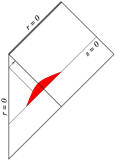
So far, we have not talked about specifics of the boundary conditions placed on the equation (35). That depends on the physical problem being considered. If the flat spacetime part $v<0$ were unperturbed, the null shell junction conditions, discussed in Appendix A, would require that $f=0$ on the surface $v=0$. If some part of the pulse propagates in the flat sector $v<0$, $f$ should be continuous across the surface $v=0$. Essentially, we can specify value of $f$ on the wedge $(v=0)\cup(s=0)$ arbitrarily, keeping in mind that perturbation value should be bounded at future infinity. It is practical to split the wavepacket to three components, as shown in Fig. 2, and consider outgoing, “constant” and incoming packets separately.

A Outgoing Wavepacket

The outgoing wavepacket is characterized by

$$f(x=0,s)=f_{O}(s),\hskip 10.00002ptf(x,s=0)=0$$ (46)

and is propagating outwards to future infinity, except for backscatter on the background curvature which goes towards the singularity at $s=+\infty$. The boundary conditions and the initial term for equation (40) are

$$F(y=1,k)=F_{O}(k),\hskip 10.00002pth(y)=0.$$ (47)

The general solution of the homogeneous form of equation (40) is

$$F(y,k)=A(k)Z_{1}(y,k)+B(k)Z_{2}(y,k),$$ (48)

where $Z_{1}$ and $Z_{2}$ are two linearly independent solutions of the homogeneous hypergeometric equation, in notation of Appendix B. To satisfy boundary conditions at $y=1$, parameters $A$ and $B$ must be

$$A(k)=F_{O}(k),\hskip 10.00002ptB(k)=0.$$ (49)

Therefore, the outgoing wavepacket solution is given by

$$f(y,s)=\frac{1}{2\pi i}\int\limits_{\kappa-i\infty}^{\kappa+i\infty}F_{O}(k){\cal F}(a,b;k;1-y)e^{ks}\,dk,$$ (50)

where ${\cal F}$ is the hypergeometric function.

If $f_{O}(s)$ does not grow exponentially as $s\rightarrow+\infty$ by itself, i.e. the image $F_{O}(k)$ does not have poles in $\text{Re}\,k>0$ half-plane, than neither does $f(y,s)$. The outgoing wavepacket just propagates harmlessly out to future infinity, never growing enough to cause significant deviation of the solution from the Roberts background.

B “Constant” Wavepacket

Even more trivial is the case of the “constant” wavepacket, characterized by

$$f(x=0,s)=C=f(x,s=0).$$ (51)

The boundary conditions and the initial term for equation (40) are

$$F(y=1,k)=C/k,\hskip 10.00002pth(y)=-C/2.$$ (52)

The general solution of equation (40) with these boundary conditions is

$$F(y,k)=A(k)Z_{1}(y,k)+B(k)Z_{2}(y,k)+\frac{C}{k-2},$$ (53)

and the boundary conditions at $y=1$ require that

$$A(k)=-\frac{2C}{k(k-2)},\hskip 10.00002ptB(k)=0.$$ (54)

So the constant wavepacket solution is given by

$$f(y,s)=\frac{C}{2\pi i}\int\limits_{\kappa-i\infty}^{\kappa+i\infty}\left[1-\frac{2}{k}\,{\cal F}(a,b;k;1-y)\right]\frac{e^{ks}}{k-2}\,dk,$$ (55)

and it does not grow as $s\rightarrow+\infty$ either.

C Incoming Wavepacket

By far, the most physically interesting case is the incoming wavepacket characterized by

$$f(x=0,s)=0,\hskip 10.00002ptf(x,s=0)=f_{I}(x).$$ (56)

It propagates directly towards the singularity and is responsible for near-critical behavior and breaking of the solution away from the Roberts background, as we shall demonstrate. The boundary conditions and the initial term for equation (40) are

$$F(x=0,k)=0,\hskip 10.00002pth(y)=-y\dot{f_{I}}(y)-f_{I}(y)/2.$$ (57)

To solve the inhomogeneous hypergeometric equation (40),

$$y(1-y)\ddot{F}+[1-(k+1)y]\dot{F}-(k/2-1)F=h,$$ (58)

with the boundary conditions

$$F(y=1,k)=0,\hskip 10.00002ptF(y=\infty,k)\text{ bounded},$$ (59)

we must construct a Green’s function out of the fundamental system of solutions of the homogeneous equation

$$Z_{1}(y) = {\cal F}(a,b;k;1-y)$$ (60)

$$Z_{2}(y) = (1-y)^{1-k}{\cal F}(1-a,1-b;2-k;1-y),$$ (61)

where parameters $a$ and $b$ of hypergeometric equation depend on $k$ as given by equation (43). The Wronskian of the above system is

$$W(y)=(k-1)y^{-1}(1-y)^{-k},$$ (62)

and the Green’s function is constructed as

$$G(y,\eta) = AZ_{1}(y)+BZ_{2}(y)\pm\frac{1}{2p_{0}(\eta)W(\eta)}\left[Z_{1}(y)Z_{2}(\eta)-Z_{2}(y)Z_{1}(\eta)\right]$$ (63)

$$= AZ_{1}(y)+BZ_{2}(y)\pm\frac{(1-\eta)^{k-1}}{2(k-1)}\left[Z_{1}(y)Z_{2}(\eta)-Z_{2}(y)Z_{1}(\eta)\right],$$ (64)

where the coefficients $A$ and $B$ are to be determined by applying the boundary conditions, and the plus-minus sign is taken depending on the arguments of the Green’s function

$$\pm=\left\{\begin{array}[]{ll}+,&1\leq y\leq\eta\\ -,&\eta\leq y<\infty\end{array}\right..$$ (65)

The Green’s function $G$ satisfies ${\cal D}_{k}G(y,\eta)=\delta(y-\eta)$, and hence can be used to construct the solution of inhomogeneous equation

$$F(y,k)=\int\limits_{1}^{\infty}G(y,\eta)h(\eta)\,d\eta$$ (66)

As the initial value problem (58) is not self-adjoint, the Green’s function (63) need not be symmetric in its arguments $y$ and $\eta$. Note that the Green’s function is calculated for particular $k$-mode, and so depends on $k$, but we omitted the third argument in $G(y,\eta;k)$ for brevity.

We now proceed to apply boundary conditions to the Green’s function (63), starting with the boundary conditions at $y=1$. The fundamental solution $Z_{1}$ goes to one there, while the behavior of $Z_{2}$ is fundamentally different depending on the sign of $\text{Re}(1-k)$. If $\text{Re}\,k<1$, the real part of power of $(1-y)$ in (60) is positive, and $Z_{2}$ goes to zero when $y=1$. If $\text{Re}\,k>1$, the real part of power of $(1-y)$ is negative, and hence $Z_{2}$ diverges when $y=1$. Substituting this into Green’s function, we get

$$G(y=1,\eta)=A+\frac{(1-\eta)^{k-1}}{2(k-1)}\,Z_{2}(\eta)+\left[B-\frac{(1-\eta)^{k-1}}{2(k-1)}\,Z_{1}(\eta)\right]\left\{\begin{array}[]{ll}0,&\text{Re}\,k<1\\ \infty,&\text{Re}\,k>1\end{array}\right\}.$$ (67)

The boundary conditions (59) require that $G(y=1,\eta)=0$, which uniquely fixes the coefficients

$$A=-\frac{(1-\eta)^{k-1}}{2(k-1)}\,Z_{2}(\eta),\hskip 10.00002ptB=\frac{(1-\eta)^{k-1}}{2(k-1)}\,Z_{1}(\eta),$$ (68)

provided $\text{Re}\,k>1$, which is precisely the region of the complex $k$-plane the contour of the inverse Laplace transformation should be in. (If $\text{Re}\,k<1$, coefficient $B$ can be arbitrary.) With these coefficients, the Green’s function (63) becomes

$$G(y,\eta)=\left\{\begin{array}[]{cl}0,&y\leq\eta\\ \frac{(1-\eta)^{k-1}}{k-1}\left[Z_{1}(\eta)Z_{2}(y)-Z_{2}(\eta)Z_{1}(y)\right],&\eta\leq y\end{array}\right..$$ (69)

The causality of wave propagation is apparent here: the wave at $y$ is only influenced by the data from the past $\eta\leq y$.

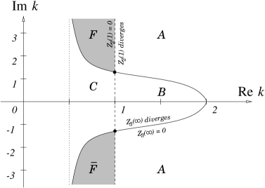
We see that the boundary conditions at $y=1$ already fix Green’s function (69), but we still have to satisfy the boundary conditions at infinity! One can show that they are satisfied automatically if (and only if) $\text{Re}\,a\geq 0$. Curves $\text{Re}\,k=1$ and $\text{Re}\,a=0$ split the complex $k$ plane into several regions, as shown in Fig. 3. The Green’s function (69) as written above is defined in region $A$, but could be analytically continued to the whole complex space. The obstructions Green’s function encounters on the boundaries between $A$ and $B$ and $A$ and $F$ are not poles, indeed, they are not even singular for regular $(y,\eta)$. They are rather caused by the fact that the Green’s function (69) fails to be applicable once you cross these boundaries; in the region $B$ boundary conditions at infinity fail to be satisfied, and in the region $F$ free modes (solutions of homogeneous equation, that is) exist that satisfy all boundary conditions, making the Green’s function not unique. The existence of free modes in region $F$ is at the heart of the matter, as they grow and will determine what will happen to the wavepacket at the later times. (It is also possible to construct Green’s function in region $C$, but since it has no bearing on our analysis, we will not do it here.)

Once Green’s function has been determined, it is simple to construct later-time evolution of the wavepacket from the initial data using equation (66)

$$F(y,k)=\int\limits_{1}^{y}\frac{(1-\eta)^{k-1}}{k-1}\left[Z_{1}(\eta)Z_{2}(y)-Z_{2}(\eta)Z_{1}(y)\right]h(\eta)\,d\eta.$$ (70)

To get back from the complex $k$-plane dependence to the physical time evolution, one performs inverse Laplace transformation

$$f(y,s)=\frac{1}{2\pi i}\,\int\limits_{\kappa-i\infty}^{\kappa+i\infty}F(y,k)e^{ks}dk.$$ (71)

We emphasize again that a particular choice of the contour of integration is not important, as long as it is to the right of the obstructions on the complex plane, in our case region $F$. In practice, one chooses the contour so that the integral (71) is easier to evaluate. For some approximation to work, the contour should touch the obstruction, which means pushing it leftwards to the very edge of region $F$ at $\text{Re}\,k=1$.

V Late-time Behavior of Incoming Wavepacket

While expressions for $f$ written down in the previous section formally solve the problem of wave propagation on the Roberts background, they are too complicated to be of practical use. In this section, we use the method of the stationary phase to obtain late-time (large $s$) asymptotic for $f(y,s)$ and analyze several physically important regimes of the wavepacket evolution.

The method of the stationary phase deals with the approximate evaluation of Fourier-type integrals

$$f(\lambda)=\int\limits_{\alpha}^{\beta}F(k)\exp[i\lambda S(k)]\,dk$$ (72)

for large positive parameter $\lambda$. It is based on a simple idea that where $\exp[i\lambda S(k)]$ is oscillating extremely rapidly and $F(k)$ is smooth, the oscillations will cancel out, and the only contributions to the integral will be from stationary points of phase $S(k)$, singular points of $F(k)$ and $S(k)$, and possibly end points.

Inverse Laplace transform integrals (38) are precisely of the above type, with phase $S(k)=k$ and large parameter $\lambda$ being the scale coordinate $s$. So the stationary phase method tells us that the asymptotic $s\rightarrow\infty$ of the solution $f(y,s)$ is given by singular points of $F(y,k)$ as a function of $k$, i.e. singular points of $G(y,\eta;k)$. Therefore the study of analytic properties of Green’s function (69) plays a key role in understanding the late-time evolution of the wavepacket. The possible sources of non-analyticity in Green’s function are listed below:

• Branch points $k=1\pm i\sqrt{3}$ of $a,b=1/2(k\pm\sqrt{k^{2}-2k+4})$

• Poles at $k=2+n$ in $Z_{2}$ and $k=-n$ in $Z_{1}$ coming from the hypergeometric function

• The pole at $k=1$ from the prefactor

• Power-law singularity of the type $(1-y)^{k-1}$

Problem with branches of the coefficients $a,b$ is absent in the Green’s function $G$ because they only enter it through the first and second arguments of the hypergeometric function, and the hypergeometric series are written in terms of $ab=k/2-1$ and $a+b=k$ only. Various poles at integer values of $k$ are all canceled out because of the antisymmetric way hypergeometric functions enter $G$. In fact, the only source of non-analyticity in $G$ is power-law singularity, and then only at $y,\eta\rightarrow 1$. Despite the appearance, $G(y,\eta;k)$ is an entire analytic function of $k$ provided that $y,\eta$ are regular points.

Since the small $\eta$ region is important for the late-time evolution of the wavepacket, it is instructive to take a closer look at the approximation to the Green’s function (69) there. Using the asymptotic behavior of $Z_{1}$, $Z_{2}$ near $\eta=1$, given in Appendix B, we obtain

$$G(y,\eta\rightarrow 1) \approx \frac{(1-\eta)^{k-1}}{k-1}\left[Z_{2}(y)-(1-\eta)^{1-k}Z_{1}(y)\right]$$ (73)

$$= \frac{1}{k-1}\left[\left(\frac{1-\eta}{1-y}\right)^{k-1}{\cal F}_{2}(y)-{\cal F}_{1}(y)\right],$$ (74)

where we introduce the short-hand notation

$${\cal F}_{1}(y) = {\cal F}(a,b;k;1-y),$$ (75)

$${\cal F}_{2}(y) = {\cal F}(1-a,1-b;2-k;1-y).$$ (76)

Note that even though poles in the hypergeometric functions no longer cancel in (73), they are purely artifacts of the approximation, and should be ignored.

Now we will use the above approximation (73) for the Green’s function to study the late-time evolution of the packet in several important regimes.

A Evolution near $v=0$

Let us first consider the behavior of the wavepacket near $y=1$, that is, near the initial null surface $v=0$. We take the asymptotic behavior of the initial term $h$ to be the fairly generic power law

$$h(\eta)\propto(1-\eta)^{\alpha},$$ (77)

which covers the usual case of functions analytic at $y=1$ (via Taylor expansion), as well as the case of functions with a power singularity at $y=1$, such as free modes $Z_{2}$. Then the approximation to the Green’s function (73) gives the solution in the desired region,

$$F(y,k)\approx\int\limits_{1}^{y}\frac{1}{1-k}\left[\left(\frac{1-\eta}{1-y}\right)^{k-1}{\cal F}_{2}(y)-{\cal F}_{1}(y)\right]\left(\frac{1-\eta}{1-y}\right)^{\alpha}(1-y)^{\alpha}\,d\eta.$$ (78)

The above integral can be explicitly evaluated using the change of variable

$$\zeta=\ln\left(\frac{1-\eta}{1-y}\right),$$ (79)

which leads to the answer

$$F(y,k) \approx -\int\limits_{-\infty}^{0}\frac{1}{1-k}\left[e^{(k-1)\zeta}{\cal F}_{2}(y)-{\cal F}_{1}(y)\right]e^{(1+\alpha)\zeta}(1-y)^{1+\alpha}\,d\zeta$$ (80)

$$= -(1-y)^{1+\alpha}\frac{1}{k-1}\left[\frac{{\cal F}_{2}(y)}{k+\alpha}-\frac{{\cal F}_{1}(y)}{1+\alpha}\right].$$ (81)

To obtain the late-time evolution of the wavepacket near $y=1$, we use the method of stationary phase. Observe that the only real singularity of $F(y,k)$ is the simple pole at $k=-\alpha$, with the rest being artifacts of the approximation (73). Therefore, the late-time behavior of the wavepacket is exponential in the scale $s$; indeed, it is given by

$$f(y,s)\approx\frac{(1-y)^{1+\alpha}}{1+\alpha}\,{\cal F}_{2}(y;-\alpha)e^{-\alpha s}=\frac{1}{1+\alpha}\,Z_{2}(y;-\alpha)\,e^{-\alpha s}.$$ (82)

There are several things worth noting about the above result. First, it gives the correct answer for the evolution of the free mode. Since $Z_{2}(y;p)\approx(1-y)^{1-p}$, the initial term works out to be $h(y)\approx(1-p)(1-y)^{-p}$, so the above formula gives $f(y,s)\approx Z_{2}(y;p)e^{ps}$, which is precisely what the evolution of the free mode should be. Second, the growing modes cannot be excited by the initial profile analytic at $y=1$. If this were the case, then $h$ could be expanded in a Taylor series around $y=1$, each term in the series raised to integer power corresponding to non-negative value of $\alpha$, and so not growing at large $s$. Third, the above argument illustrates how only the $Z_{2}$ content of the initial data is relevant to the subsequent evolution of the wavepacket.

So it seems that the exponential growth of the wavepacket at late times must be already built into the initial data in form of a power-law divergence of the initial wave profile, just as it is encoded in the pure free mode $Z_{2}$. But a power-law divergence of the perturbation near $v=0$ causes curvature invariants to diverge at the junction, making the surface $v=0$ a weak null singularity, which casts a shadow of doubt on the physicality of such growing modes. The question then arises whether it is possible to somehow eliminate the offending divergence, while still having a wavepacket grow to large enough values. The answer to this question is yes, and it is discussed next.

B Evolution of a wavepacket initially localized at $v=0$

So what will happen if we cut off a diverging initial wave shape (77) below some small value of $y-1$, say $\lambda$? To put it in another way, will the power-law diverging wave localized near $y=1$ backscatter and affect the evolution of the wavepacket at the large $y$? If not, then subtracting such localized wavepacket from perturbation modes discussed above will cut off the divergence at $y=1$, while keeping the rest of the wavepacket evolution essentially unchanged.

We model such a localized wave by adding an exponential cutoff to the generic power law initial term (77)

$$h(\eta)\propto(1-\eta)^{\alpha}e^{(1-\eta)/\lambda}.$$ (83)

The exponential factor is chosen because it effectively suppresses $h$ for values of $y-1>\lambda$, yet still keeps the calculations simple. We are interested in the evolution of the wavepacket well outside the region of initial localization, but still for small enough $y$ so that approximation (73) holds, that is for $\lambda\ll y-1\ll 1$ (that can always be arranged for small enough $\lambda$). In this region of interest we have

$$F(y,k)\approx\int\limits_{1}^{y}\frac{1}{1-k}\left[\left(\frac{1-\eta}{1-y}\right)^{k-1}{\cal F}_{2}(y)-{\cal F}_{1}(y)\right](1-\eta)^{\alpha}e^{(1-\eta)/\lambda}\,d\eta.$$ (84)

The above integral can be evaluated by the change of variable

$$t=\frac{\eta-1}{\lambda},$$ (85)

which yields the following approximation for $F(y;k)$ in the region of interest:

$$F(y,k) \approx \int\limits_{0}^{\infty}\frac{1}{1-k}\left[\left(\frac{-\lambda t}{1-y}\right)^{k-1}{\cal F}_{2}(y)-{\cal F}_{1}(y)\right](-\lambda t)^{\alpha}e^{-t}\,\lambda dt$$ (86)

$$= -\frac{1}{k-1}\left[(-\lambda)^{k+\alpha}\Gamma(k+\alpha)(1-y)^{1-k}{\cal F}_{2}(y)-(-\lambda)^{1+\alpha}\Gamma(1+\alpha){\cal F}_{1}(y)\right].$$ (87)

So outside the region of initial localization of the wavepacket, but still for small $y$, the Laplace transform of the field perturbation is approximately given by

$$F(y,k)\approx-\frac{1}{k-1}\left[(-\lambda)^{k+\alpha}\Gamma(k+\alpha)Z_{2}(y)-(-\lambda)^{1+\alpha}\Gamma(1+\alpha)Z_{1}(y)\right].$$ (88)

The main contribution to the late-time behavior is coming from the poles of the gamma-function $\Gamma(k+\alpha)$ in the first term. Using the stationary phase approximation, it is possible to calculate this contribution exactly. The inverse Laplace transform of $F(y;k)$ can be reduced to the inverse Mellin transform of the gamma-function

$$f(y,s) \approx \frac{1}{2\pi i}\,\int\limits_{\kappa-i\infty}^{\kappa+i\infty}\frac{Z_{2}(y;-\alpha)}{1+\alpha}\,\lambda^{k+\alpha}\Gamma(k+\alpha)e^{ks}dk$$ (89)

$$= \frac{Z_{2}(y;-\alpha)}{1+\alpha}\,\frac{e^{-\alpha s}}{2\pi i}\,\int\limits_{\kappa+\alpha-i\infty}^{\kappa+\alpha+i\infty}\lambda^{k}\Gamma(k)e^{ks}dk$$ (90)

$$= \frac{Z_{2}(y;-\alpha)}{1+\alpha}\,\frac{e^{-\alpha s}}{2\pi i}\,\int\limits_{\kappa+\alpha-i\infty}^{\kappa+\alpha+i\infty}\Gamma(k)\left[e^{-(s+\ln\lambda)}\right]^{-k}dk$$ (91)

$$= \frac{Z_{2}(y;-\alpha)}{1+\alpha}\,e^{-\alpha s}\,[{\cal M}^{-1}\Gamma]\left(e^{-(s+\ln\lambda)}\right),$$ (92)

which is a known integral; indeed, $[{\cal M}^{-1}\Gamma](x)=e^{-x}$. Therefore we obtain the following late-time approximation of the field perturbation outside the region of initial localization:

$$f(y,s)\approx\frac{\Theta(s+\ln\lambda)}{1+\alpha}\,Z_{2}(y;-\alpha)\,e^{-\alpha s}.$$ (93)

This looks very similar to the earlier result (82); the only difference is the factor $\Theta(s+\ln\lambda)$, where $\Theta$ is defined by

$$\Theta(x)=\exp\left[-e^{-x}\right],$$ (94)

and is almost a step function, rapidly changing its value from $0$ to $1$ as its argument becomes positive

$$\Theta(x)\approx\left\{\begin{array}[]{ll}1,&\text{Re}\,x>0\\ 0,&\text{Re}\,x<0\end{array}\right.,$$ (95)

where the width of the transition is of order unity. This means that the perturbation outside the region of initial localization does not feel the effect of the field at $y-1<\lambda$ until a much later time, namely $s=-\ln\lambda$, when it suddenly spreads. To put it simply, the wavepacket initially localized at $v<\lambda$ does not backscatter until it hits the singularity at $u=0$, and then goes out in a narrow band $-u<\lambda$.

The above result shows how we can cut off the free mode $Z_{2}(y;k)$ to avoid the curvature divergence, and yet have it grow sufficiently large. To quantify how large can it grow, consider the free mode $f=Z_{2}(y;k)e^{ks}\approx(1-y)^{1-k}e^{ks}$, with divergent scalar curvature $R\propto f^{\prime}$, and cut it off at $y-1<\lambda$. The largest initial curvature value is of order $R\propto\lambda^{-k}$, while the initial energy of the pulse is $\lambda R\propto\lambda^{1-k}$, and can be made arbitrarily small. The perturbation mode will grow exponentially until the cutoff backscatters at $s=-\ln\lambda$, at which time its amplitude will be $\lambda^{-k}$, with proportionally large curvatures and energies. In other words, the initial large curvature seed localized in a small region spreads over the whole space in the course of the evolution, with the energy of the pulse growing correspondingly. Thus, the free perturbation modes considered here are physical and grow exponentially to very large amplitudes, certainly enough to leave the linear regime, and are therefore responsible for the evolution of the solution away from the Roberts one.

C Generic initial conditions

We now turn our attention to the evolution of the wavepacket from generic initial conditions. It is reasonable to expect that completely generic initial conditions will have non-zero content of all perturbation modes present in the system, both growing and decaying, as given by equations (70) and (71),

$$f(y,s)=\int\limits_{\kappa-i\infty}^{\kappa+i\infty}\left[W_{2}(k)Z_{2}(y;k)+W_{1}(k)Z_{1}(y;k)\right]e^{ks}dk.$$ (96)

However, decaying modes will disappear very quickly, so only the growing modes are relevant to late-time evolution. Assuming that the content of the free growing mode $Z_{2}(y;k)$ is given by the weight function $W(k)$, the generic wavepacket evolution is given by the sum of all such modes

$$f(y,s)=\int\limits_{\Gamma}W(k)Z_{2}(y;k)e^{ks}dk,$$ (97)

where the infinite contour of integration $\Gamma$ runs vertically in the regions $F$ and $\bar{F}$ of the complex plane on Fig. 3, at $\text{Re}\,k=1$. However, we note that the part of the contour between endpoints $k_{0}^{\pm}=1\pm i\sqrt{2}$ of the regions $F$ and $\bar{F}$ does not correspond to free growing modes, as $Z_{2}(y\rightarrow\infty)\approx(-y)^{-a}$ with $\text{Re}\,a<0$ there, and so boundary conditions at infinity are not satisfied. Therefore, for the initial wavepacket bounded at infinity, the content of such modes is suppressed, so that $\int dk\,[W(k)\,(-y)^{-a}]\sim 1$ for large $y$. This leads to slower growth rates $\int dk\,[W(k)\,(-ye^{s})^{-a}e^{(k+a)s}]\sim e^{(\kappa+a)s}$ at the later times. Hence, the piece of the contour $\Gamma$ between the endpoints $k_{0}^{\pm}$ can be omitted from the integration without affecting the late-time evolution.

For completely generic initial conditions, we should expect $W$ to be a smooth function of $k$ in the free mode region $F$, not preferring any particular value of $k$. Therefore, using the stationary phase approximation, the main contribution to the late-time behavior of the above integral comes from the end points of the contour of integration,

$$f(y,s)\approx-W(k_{0}^{+})Z_{2}(y;k_{0}^{+})\,\frac{e^{k_{0}^{+}s}}{s}-W(k_{0}^{-})Z_{2}(y;k_{0}^{-})\,\frac{e^{k_{0}^{-}s}}{s}.$$ (98)

Ignoring the overall weight factor, we find that the late-time evolution of the generic wavepacket is given by

$$f(y,s)\propto\text{Re}\left[Z_{2}(y;k_{0})\,\frac{e^{k_{0}s}}{s}\right].$$ (99)

We emphasize that the single $k_{0}$-mode dominates the course of evolution of the generic wavepacket, and thus a certain universality is present in the way a generic perturbation departs from the Roberts solution.

VI Discussion

In this paper, we studied spherically symmetric perturbations of the Roberts solution with the intent to understand how nearby solutions depart from the Roberts one in the course of the field evolution, and what bearing the Roberts solution has on the subject of critical phenomena in general, and how it is related to Choptuik’s critical solution in particular. We analyzed the behavior of incoming and outgoing wavepackets, and we focused our attention on the incoming one as the physically relevant one for the question posed. With the aid of the Green’s function formulation, we were able to completely solve the perturbation problem in closed form, as well as obtain simple approximations for the late-time evolution of the field in several important regimes.

As was shown above, the departure of the generic perturbation away from the Roberts solution is universal in a sense that the single mode $Z_{2}(y;k_{0})e^{k_{0}s}$ dominates the late-time evolution of the field. The complex growth exponent gives rise to an interesting physical effect: the perturbation developing on the scale-invariant background evolves to have a scale-dependent structure $e^{s}\cos(\text{Im}\,k_{0}s)$. The exponential growth of the amplitude of the perturbation will eventually be stopped by the non-linear effects, while the periodic dependence of the perturbation on the scale will most likely remain. The period of oscillation, obtained in the linear approximation, is

$$\Delta=\frac{2\pi}{\text{Im}\,k_{0}}.$$ (100)

What does this periodic dependence of the solution on the scale mean physically? To answer this question, lets see how this symmetry is expressed in the Schwarzschild coordinates $(r,t)$ often used in numerical calculations (see, for example, [1]). In this coordinates the metric (5) is diagonal

$$ds^{2}=-\alpha\,dt^{2}+\beta\,dr^{2}+r^{2}\,d\Omega^{2},$$ (101)

where metric coefficients and explicit expressions for coordinates are given in Appendix C. For our purposes, it suffices to note that the coordinate $x$ determines the ratio $r/t$, while the coordinate $s$ sets an overall scale of both space and time coordinates via $e^{-s}$ factor

$$-\,\frac{r}{t}=\exp\left[x+\frac{1}{2}\,e^{2x}\right],\hskip 10.00002ptr=\exp[x-s].$$ (102)

One can see that taking a step $\Delta$ in the scale variable $s$ is equivalent to scaling both spatial and time coordinates $r$ and $t$ down by a factor $e^{\Delta}$. Therefore, the solution being periodic in scale coordinate $s$ is equivalent to being invariant under rescaling of space and time coordinates $r$ and $t$ by a certain factor

$$f(x,s+\Delta)=f(x,s)\ \Longleftrightarrow\ f(e^{-\Delta}r,e^{-\Delta}t)=f(r,t).$$ (103)

The later is an expression of the symmetry observed in the numerical simulations of the massless scalar field collapse [1], and referred to as echoing, or discrete self-similarity in the literature [1, 7].

Thus, our simple analytical model of the critical collapse of the massless scalar field illustrates how the continuous self-similarity of the Roberts solution is dynamically broken to discrete self-similarity by the growing perturbations, reproducing the essential feature of numerical critical solutions. The value of exponent for the endpoints of the spectrum of growing perturbation modes, $k_{0}=1+i\sqrt{2}$, gives the period of discrete self-similarity as

$$\Delta=\sqrt{2}\pi=4.44$$ (104)

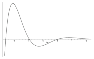
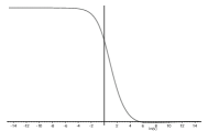
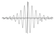
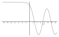
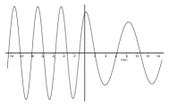
for linear perturbations of the Roberts solution, which is within $25\%$ of the numerical value $\Delta=3.44$ measured by Choptuik [1]. Given that the perturbative model considered here reproduces all the symmetries of the Choptuik’s solution, and gives a good estimate for the period of echoing, it is instructive to compare the actual field profiles to the numerical calculations. There are some technical issues connected with rewriting our results in the variables Choptuik uses, which are addressed in Appendix C, but the end result of calculation for field variable $X=\sqrt{2\pi}\,\sqrt{\frac{r^{2}}{\alpha}}\,\frac{\partial\phi}{\partial r}$ from the perturbation modes is presented in Fig. 5. Comparing this plot to Fig. 2 in original Choptuik’s paper [1], we see that they share one common feature, which is the oscillatory nature of the field solution; however, the shape of the field profiles is quite different. This discrepancy is not surprising, however, since perturbation methods in critical phenomena are usually viable for calculating critical exponents, but not the field configurations themselves.

The emerging discretely self-similar structure, and the universal way in which the generic perturbation departs away from the Roberts solution offer support for the conjecture that the Roberts solution is “close” to the Choptuik one in the phase space of all massless scalar field configurations (in a sense of being in the basin of attraction of the latter), and will evolve towards it when perturbed [14]. It seems highly unlikely, however, that the critical mode responsible for the decay of the Choptuik solution will be completely absent in the initial data originating near the Roberts solution, as this usually requires fine-tuning of the parameters. So though at first the field configuration near the Roberts solution might seem to evolve towards the Choptuik solution, after a while the critical mode will kick in and drive the field to either dispersal or black hole formation. This picture is in line with the Choptuik solution being intermediate attractor, and we offered “ball rolling down the stairs” analogy earlier [14] to visualize the field evolution as it goes from initial configuration (the Roberts solution) to local attractor (the Choptuik solution) and then to global attractor (black hole or flat spacetime) in the phase space. Unfortunately, linear perturbation methods are not sufficient to provide a proof of the proposed scenario, and fail to give the answer as to what would the eventual fate of the evolution be (whether black hole or flat spacetime end-state will be selected), and how fast would the field get there.

To completely answer these questions, one would need to employ some sort of non-linear calculation, or perform numerical simulations of the evolution. In particular, it would be interesting to evolve the perturbed Roberts spacetime numerically and look for the Choptuik spacetime as the possible intermediate attractor. Nevertheless, it may happen that some information about Choptuik’s solution can be gained from the linear perturbation analysis of the Roberts solution. The appeal of this method lies in the fact that such analysis could be carried out analytically, while Choptuik’s solution is still unknown in the closed form. Similarly, one can try to study properties of other analytically-unknown critical solutions in different matter models based on “nearby” solutions with higher symmetry and simpler form. One might also hope to obtain acceptable analytical approximations to critical solutions, Choptuik’s in particular, by going to higher order perturbation theory in the region near the singularity.

To summarize, our main result is the dynamical explanation of how discretely self-similar structure forms on the continuously self-similar background in the collapse of the minimally-coupled massless scalar field, and the prediction for the period of this structure $\Delta=\sqrt{2}\pi=4.44$, which is quite close to the numerical value $\Delta=3.44$, considering we only did a first-order perturbation analysis, and that non-linear effects can, in principle, renormalize that value.

A Null Shell Junction Conditions

The influx of the scalar field in the Roberts solution is turned on at the advanced time $v=0$, with the spacetime being flat before that. In this appendix, we consider in detail junction condition across this null surface, and their implications for boundary conditions of perturbation problem. This discussion is adopted from general treatment of thin null shells by Barrabès and Israel [15].

Consider the general spherically symmetric metric in null coordinates

$$ds^{2}=-2e^{2\sigma}\,du\,dv+r^{2}\,d\Omega^{2}.$$ (A1)

To fix the geometry of the soldering of spherically symmetric spacetimes uniquely, one must match radial functions across the constant advanced time hypersurface. To this end, we rewrite the above metric in terms of advanced Eddington coordinates on both sides

$$ds^{2}=-e^{\psi}\,dv\,(fe^{\psi}\,dv-2\,dr)+r^{2}\,d\Omega^{2}.$$ (A2)

The metric coefficients in Eddington coordinates can be calculated from those in null coordinates by

$$e^{\psi}=-\frac{e^{2\sigma}}{r_{,u}},\hskip 10.00002ptf=-2\,\frac{r_{,u}r_{,v}}{e^{2\sigma}}.$$ (A3)

The surface density and pressure of the null shell are then determined by jumps of the metric coefficients across the $v=\text{const}$ surface

$$4\pi r^{2}\epsilon=[m],\hskip 10.00002pt8\pi P=[\psi_{,r}],$$ (A4)

where the local mass function $m(v,r)$ is introduced, as usual, by

$$f=1-\frac{2m}{r}.$$ (A5)

For Minkowski spacetime $f=1$ and $\psi=\text{const}$, so below the $v=0$ hypersurface surface we have

$$m(v<0)=0,\hskip 10.00002pt\psi_{,r}(v<0)=0.$$ (A6)

For the Roberts solution (5,6), we have $\sigma=0$, $r^{2}=u^{2}-uv$, so a direct calculation gives

$$m=-\frac{uv}{4r},\hskip 10.00002pt\psi_{,r}=\frac{1}{r}\,\frac{v^{2}}{4r^{2}+v^{2}}.$$ (A7)

Obviously,

$$\lim_{v\rightarrow+0}m=0,\hskip 10.00002pt\lim_{v\rightarrow+0}\psi_{,r}=0,$$ (A8)

so the Roberts solution is indeed attached smoothly to the flat spacetime, without a delta function-like stress-energy tensor singularity associated with a massive null shell.

If one wishes to attach a perturbed Roberts spacetime to the flat one, as we do, and still have no singularity at the junction, the null shell matching conditions above will place boundary conditions on the perturbation values at the junction surface. To obtain these, we take the perturbed Roberts solution in null gauge of Ref. [12], given by $\sigma=\sigma(x)e^{ks}$, $r=e^{x-s}(1+\rho(x)e^{ks})$, and calculate the null shell surface density

$$[m]=[-\rho^{\prime}/2+(k/2-1)\rho+\sigma]e^{(k-1)s}$$ (A9)

and surface pressure

$$[\psi_{,r}]=-k[(k-1)\rho+2\sigma]e^{(k+1)s}.$$ (A10)

The simultaneous vanishing of these two for arbitrary $k$ can only be accomplished if

$$\rho=\rho^{\prime}=\sigma=0,$$ (A11)

and these are precisely the boundary conditions we imposed on metric coefficients earlier. One also has to require continuity of the scalar field across junction, so the boundary condition on scalar field perturbation is

$$\phi=0.$$ (A12)

These boundary conditions on perturbations in the null gauge simply mean vanishing of gauge-invariant perturbation amplitudes (defined in the next appendix) on the $v=0$ hypersurface.

B Properties of the Hypergeometric Equation

We showed above that the linear perturbation analysis of the Roberts solution can be reduced to the study of solutions of the hypergeometric equation with certain parameters. The hypergeometric equation has been extensively studied; for a complete description of its main properties see, for example, [16]. In this appendix we collect the facts about the hypergeometric equations that are of immediate use to us, mainly to establish notation.

The hypergeometric equation is a second order linear ordinary differential equation,

$$y(1-y)\ddot{Z}+[c-(a+b+1)y]\dot{Z}-abZ=0,$$ (B1)

with parameters $a$, $b$, and $c$ being arbitrary complex numbers. It has three singular points at $y=0,1,\infty$. Its general solution is a linear combination of any two different solutions from the set

$$Z_{1} = {\cal F}(a,b;a+b+1-c;1-y),$$ (B2)

$$Z_{2} = (1-y)^{c-a-b}{\cal F}(c-a,c-b;c+1-a-b;1-y),$$ (B3)

$$Z_{3} = (-y)^{-a}{\cal F}(a,a+1-c;a+1-b;y^{-1}),$$ (B4)

$$Z_{4} = (-y)^{-b}{\cal F}(b+1-c,b;b+1-a;y^{-1}),$$ (B5)

$$Z_{5} = {\cal F}(a,b;c;y),$$ (B6)

$$Z_{6} = y^{1-c}{\cal F}(a+1-c,b+1-c;2-c;y),$$ (B7)

where ${\cal F}(a,b;c;y)$ is the hypergeometric function, defined by the power series

$${\cal F}(a,b;c;y)=\sum\limits_{n=0}^{\infty}\frac{(a)_{n}(b)_{n}}{(c)_{n}}\,\frac{y^{n}}{n!},$$ (B8)

and we used shorthand notation $(a)_{n}=\Gamma(a+n)/\Gamma(a)$. The hypergeometric series is regular at $y=0$, its value there is ${\cal F}(a,b;c;0)=1$, and it is absolutely convergent for $|y|<1$. Considering the hypergeometric series as a function of its parameters, one can show that ${\cal F}(a,b;c;y_{0})/\Gamma(c)$ is entire analytical function of $a$, $b$, and $c$, provided that $|y_{0}|<1$.

The solutions $Z_{1},\ldots,Z_{6}$ are based around different singular points of the hypergeometric equation, with asymptotics given by

$$Z_{1}=1,\ Z_{2}=(1-y)^{c-a-b} y=1,$$ near (B9)

$$Z_{3}=(-y)^{-a},\ Z_{4}=(-y)^{-b} y=\infty,$$ near (B10)

$$Z_{5}=1,\ Z_{6}=y^{1-c} y=0.$$ near (B11)

Any three of the functions $Z_{1},\ldots,Z_{6}$ are linearly dependent with constant coefficients. In particular,

$$\left[\begin{array}[]{c}Z_{1}\\ Z_{2}\end{array}\right]=\left[\begin{array}[]{cc}c_{13}&c_{14}\\ c_{23}&c_{24}\end{array}\right]\left[\begin{array}[]{c}Z_{3}\\ Z_{4}\end{array}\right],$$ (B12)

where the coefficient matrix is given by

$$\left[\begin{array}[]{cc}c_{13}&c_{14}\\ c_{23}&c_{24}\end{array}\right]=\left[\begin{array}[]{cc}\frac{\Gamma(a+b+1-c)\Gamma(b-a)}{\Gamma(b+1-c)\Gamma(b)}\,e^{-i\pi a}&\frac{\Gamma(a+b+1-c)\Gamma(a-b)}{\Gamma(a+1-c)\Gamma(a)}\,e^{-i\pi b}\\ \frac{\Gamma(c+1-a-b)\Gamma(b-a)}{\Gamma(1-a)\Gamma(c-a)}\,e^{-i\pi(c-b)}&\frac{\Gamma(c+1-a-b)\Gamma(a-b)}{\Gamma(1-b)\Gamma(c-b)}\,e^{-i\pi(c-a)}\\ \end{array}\right].$$ (B13)

These relationships are true for all values of the parameters for which the gamma-function terms in the numerators are finite, and all values of $y$ for which corresponding series converge, with $\text{Im}\,y>0$. If $\text{Im}\,y<0$, signs of arguments in the exponential multipliers should be inverted. We shall not give the rest of similar relationships here.

C Spacetime in Curvature Coordinates

For comparison of our results to Choptuik’s numerical simulations [1], we must rewrite them in the diagonal Schwarzschild-like coordinates Choptuik uses

$$ds^{2}=-\alpha\,dt^{2}+\beta\,dr^{2}+r^{2}\,d\Omega^{2}.$$ (C1)

One can straightforwardly check that the coordinate change

$$t=-\exp\left[-s-\frac{1}{2}\,e^{2x}\right],\hskip 10.00002ptr=\exp[x-s]$$ (C2)

diagonalizes the Roberts metric (9). By self-similarity, the quantity $t/r$, as well as the metric coefficients $\alpha$ and $\beta$ do not depend on the scale $s$, but only on the coordinate $x$. The metric coefficients, written as functions of $x$, are

$$\alpha=2\,\frac{\exp[e^{2x}]}{1+e^{2x}},\hskip 10.00002pt\beta=2\,\frac{1}{1+e^{-2x}}.$$ (C3)

If one wishes, one can rewrite them as explicit functions of $t/r$, using

$$x=\frac{1}{2}\,\ln W(r^{2}/t^{2}),$$ (C4)

in terms of Lambert’s $W$-function, which is defined by the solution of transcendental equation

$$W\exp(W)=x.$$ (C5)

The expressions for metric coefficients are then

$$\alpha=2\,\frac{\exp[W(r^{2}/t^{2})]}{1+W(r^{2}/t^{2})},\hskip 10.00002pt\beta=2\,\frac{W(r^{2}/t^{2})}{1+W(r^{2}/t^{2})}.$$ (C6)

However, the coefficients $\alpha$ and $\beta$ cannot be written in closed form in terms of elementary functions of $t/r$.

As you can see from expressions for the metric above, diagonal Schwarzschild coordinates are not particularly well-suited for description of the Roberts spacetime. On top of the complicated metric form, one artifact of the diagonal coordinate system is that the null singularity at $u=0$ gets compressed into a point at $r=t=0$. Also, slices $t=\text{const}$ cut across the $v=0$ hypersurface, so one has to be careful with discontinuities of the solution there.

The perturbation amplitudes in the gauge preserving diagonal form of the metric are also quite complicated. The simplest way to get them from gauge-invariant quantities is to explicitly a find gauge transformation

$$\xi^{\mu}=\left(A,B,0,0\right)$$ (C7)

connecting the simple field gauge $K=k_{vv}=0$ with the diagonal gauge, fixed by conditions $K=0$ and $(2u-v)^{2}k_{vv}=u^{2}k_{uu}$. The effects of the gauge transformation on the perturbation amplitudes were given above in Section III. Imposing the condition $K=0$, one finds that $B$ must be related to $A$ by

$$B=\frac{2u-v}{u}\,A.$$ (C8)

$A$ is then found by imposing the other condition fixing diagonal gauge, which leads to the following equation

$$(2u-v)^{2}A_{,v}-u(2u-v)A_{,u}-vA=2u\int f\,dv.$$ (C9)

Rewriting A in scaling coordinates,

$$A(y,s)={\cal A}(y)e^{(k-1)s},$$ (C10)

transforms the above equation into the ordinary differential equation

$$(1+y)\dot{\cal A}+[1-k/2\,(1+y)]{\cal A}=-\int F\,dy,$$ (C11)

which can be easily solved to give

$${\cal A}(y)=-\frac{e^{\frac{k}{2}\,y}}{1+y}\,\int\limits_{1}^{y}d\xi\,e^{-\frac{k}{2}\,\xi}\int\limits_{1}^{\xi}F(\zeta)\,d\zeta.$$ (C12)

Once the connecting gauge transformation is known, it is trivial to obtain the perturbation amplitudes in the Schwarzschild diagonal gauge. In particular, the scalar field perturbation is given by

$$\varphi(y;k)=-F(y;k)+{\cal A}(y;k).$$ (C13)

We end this section by observing that while the gauge transformation term $A$ is a small correction to gauge-invariant quantities near $y=1$, it is not at all well behaved at infinity. Indeed, it blows up exponentially as $e^{\frac{k}{2}\,y}$! The presence of this gauge artifact in the quite sensibly-looking diagonal gauge illustrates just how easily one can get into trouble if one is not working in a gauge-invariant formalism.

(null coordinates)	(scaling coordinates)

FIG. 1.: Global structure of the Roberts solution: The scalar field influx is turned on at $v=0$; spacetime is flat before that. The field evolution occurs in the shaded region of the diagram, and there is a null singularity in the center of the spacetime.

outgoing	“constant”	incoming

FIG. 2.: Wave propagation on the Roberts background: Initial conditions can be equivalently specified on the surface $s=0$ extending to the center of the flat part of spacetime ($r=0$), or on the $(x=0)\cup(s=0)$ wedge. By linearity, the wavepacket can be decomposed into three modes: outgoing, “constant”, and incoming.

FIG. 3.: Complex perturbation spectrum. Values of $k$ to the left of the solid line are prohibited by the boundary conditions at infinity, to the right of the broken line by the initial conditions at $y=1$. Values in the region of intersection (the shaded regions $F$ and $\bar{F}$) are allowed, and constitute the perturbation spectrum.

$Z_{1}$	$Z_{2}$

(a) $k=\frac{3}{4}+3i$

$Z_{1}$	$Z_{2}$

(b) $k=1+i\sqrt{2}$

FIG. 4.: Field perturbation profiles on a slice $u=\text{const}$: (a) for a typical value of $k$ inside region $F$, (b) for a value of $k$ at the endpoint of region $F$. The horizontal coordinate on the plots is $\ln v$.

FIG. 5.: Profile for the field variable $X=\sqrt{2\pi}\,\sqrt{\frac{r^{2}}{\alpha}}\,\frac{\partial\phi}{\partial r}$ on the slice $t=\text{const}$ for the dominant mode $f(y,s)=Z_{2}(y;k_{0})\,e^{ks}/s$. Compare this plot to Fig. 2 of Choptuik’s paper [1].

REFERENCES

- [1] M. W. Choptuik, Phys. Rev. Lett. 70, 9 (1993).
- [2] A. M. Abrahams and C. R. Evans, Phys. Rev. Lett. 70, 2980 (1993).
- [3] C. R. Evans and J. S. Coleman, Phys. Rev. Lett. 72, 1782 (1994).
- [4] T. Koike, T. Hara, and S. Adachi, Phys. Rev. Lett. 74, 5170 (1995).
- [5] D. Maison, Phys. Lett. B366, 82 (1996).
- [6] T. Hara, T. Koike, and S. Adachi, gr-qc/9607010, 1996.
- [7] C. Gundlach, Adv. Theor. Math. Phys. 2, 1 (1998).
- [8] C. Gundlach, Phys. Rev. D 55, 695 (1997).
- [9] M. D. Roberts, Gen. Relativ. Gravit. 21, 907 (1989).
- [10] P. R. Brady, Class. Quant. Grav. 11, 1255 (1994).
- [11] Y. Oshiro, K. Nakamura, and A. Tomimatsu, Prog. Theor. Phys. 91, 1265 (1994).
- [12] A. V. Frolov, Phys. Rev. D 56, 6433 (1997).
- [13] A. V. Frolov, Class. Quant. Grav. 16, 407 (1999).
- [14] A. V. Frolov, Phys. Rev. D 59, 104011 (1999).
- [15] C. Barrabès and W. Israel, Phys. Rev. D 43, 1129 (1991).
- [16] H. Bateman and A. Erdélyi, Higher Transcendental Functions (McGraw-Hill, New York, 1953).