Quasi-Normal Modes of General Relativistic Superfluid Neutron Stars

Abstract

We develop a general formalism to treat, in general relativity, the linear oscillations of a two-fluid star about static (non-rotating) configurations. Such a formalism is intended for neutron stars, whose matter content can be described, as a first approximation, by a two-fluid model: one fluid is the neutron superfluid, which is believed to exist in the core and inner crust of mature neutron stars; the other fluid is a conglomerate of all other constituents (crust nuclei, protons, electrons, etc…). We obtain a system of equations which govern the perturbations both of the metric and of the matter variables, whatever the equation of state for the two fluids. As a first application, we consider the simplified case of two non-interacting fluids, each with a polytropic equation of state. We compute numerically the quasi-normal modes (i.e. oscillations with purely outgoing gravitational radiation) of the corresponding system. When the adiabatic indices of the two fluids are different, we observe a splitting for each frequency of the analogous single fluid spectrum. The analysis also substantiates the claim that w-modes are largely due to spacetime oscillations.

I Introduction

A formalism is presented here for describing the equilibrium configurations and quasi-normal modes of general relativistic neutron stars taking into account superfluidity. There are both theoretical and observational reasons for believing that neutron stars have superfluid interiors. On the theoretical side, nuclear physics calculations [1] indicate that the densities in neutron stars are favorable to the formation of ${}^{1}S_{0}$ neutron condensates in the neutron star crusts, with ${}^{3}P_{2}$ neutron condensates forming, as well as ${}^{1}S_{0}$ proton condensates (and perhaps even kaon and pion condensates), in the inner core. On the observational side, there is the well-established glitch phenomenon, the best description of which is based on superfluidity and quantized vortices [2]. Cooling rates for neutron stars are also best described by superfluidity [3].

There are several distinct ways in which a superfluid can differ from an ordinary perfect fluid. The most striking is that (pure) superfluids are completely free of viscous effects and are locally irrotational. The latter property is however compensated by the possibility for the superfluid to be threaded by quantized vortices, so that it can on macroscopic scales mimic the rotational behaviour of an ordinary fluid.

In the context of neutron stars, one can distinguish three main fluid constituents: the neutrons, which can either belong to nuclei in the crust or be free and superfluid in the inner crust and the core; the protons, belonging only in nuclei in the crust and in a superconducting state in the core; and finally the electrons which behave everywhere in the star as a normal fluid. As mentioned before, because of rotation, the neutron superfluid will contain vortices, whereas, because of the neutron star magnetic field, the proton superconductor is believed to contain magnetic fluxoids (at least if the core protons behave as a type II superconductor, which is the favored scenario [4]). Finally, the whole picture is complicated by the entrainment effect (misleadingly called “drag effect” in the literature) between superconducting protons and superfluid neutrons, by which the momentum of one constitutent carries some mass current of the other constituent along with it (see e.g. [4]). The theoretical description of such mixtures, including the average effect of vortices (and fluxoids) was given by Lindblom and Mendell [5, 6] in the Newtonian context, and more recently, by Carter and Langlois [7, 8] in the general relativistic context.

In many astrophysical applications, the above picture can fortunately be simplified. Indeed, it has been shown that although the protons are superconducting, they are coupled to the “normal” electron fluid on a very short timescale [9]. This implies, in practice, that the neutron star interior can be described, as a first step beyond the perfect fluid approximation, as a two-fluid model with a neutron superfluid component and a “normal” component containing everything else, i.e. the crust nuclei, the superconducting protons and the electrons. Such a two-fluid description was presented by Langlois et al [10] in a general relativistic framework. The corresponding formalism was based on a formally analogous but physically different model due to Carter (see, for instance, [11] and [12]). The purpose of Carter’s model was to extend to the general relativistic regime the non-relativistic two-fluid model of Landau (see [13]), in which the “normal” fluid is constituted of excitations (phonons, rotons, etc.) of the condensate due to non-zero temperature. In the case of neutron stars, the internal temperature is believed to decrease rather quickly after their birth to temperatures well below the nuclear temperature scale (1 MeV), so that it will be justified, at least for the global structure of the star, to ignore the temperature effects.

The effect of superfluidity on the oscillations of neutron stars has been investigated by Lindblom and Mendell [14] in a Newtonian formalism. Although analytical solutions for simple models revealed the existence of a new class of modes, which could be named superfluid modes, their numerical investigation [14] led only to ordinary modes almost indistinguishable from those obtained by a single fluid treatment, with no sign of superfluid modes. However, a subsequent numerical treatment by Lee [15], still in the Newtonian regime, was successful in extracting the superfluid modes.

The main objective of the present work is, in the same spirit as [14, 15], to investigate the influence of superfluidity on the oscillations of neutron stars in the general relativistic context. The description of oscillations in general relativity is complicated essentially by two factors: the first is that gravity is described by several components of the metric instead of the single gravitational potential of Newtonian gravity; the second is that oscillation of the star implies emission of gravitational radiation, and therefore the oscillating solutions are damped (they are called quasi-normal modes instead of normal modes).

Due to the difficulties inherent to general relativity, we shall restrict our analysis to idealized models. First, we consider only non-rotating neutron stars. Second, for the numerical application, we consider an oversimplified situation in which the two fluids exist throughout the star (i.e. without taking into account the crust-core boundary, neutron drip) and are characterized by (independent) polytropic equations of state. One of the fluids will be composed of neutrons, and the other will be a conglomerate made of protons and electrons, which we will call, loosely, “proton” fluid for simplicity in the rest of this paper.

The changes to the dynamics of the neutron star due to the existence of two fluids will be extracted to linear order via an analysis of the quasi-normal modes. The linearized metric and matter variables will be decomposed into their respective “even” and “odd” parity components. This will generalize to the two-fluid case much of the previous work (e.g. [16, 17, 18, 19, 20, 21, 22, 23]) that has been done for the one-fluid case. The present work can also be viewed as a first step in carrying over to the general relativistic regime the pioneering calculations of Lindblom and Mendell [5, 6, 14, 24] for superfluid neutron stars in the non-relativistic regime.

In Sec. II we describe the superfluid formalism. In Sec. III we show how to construct equilibrium configurations. In Sec. IV we give the linearized field equations for purely radial and non-radial oscillations inside the star and for the vacuum outside the star. The notation follows as closely as possible that used by [16, 17]. In Sec. V the boundary conditions, numerical techniques, and quasi-normal mode (QNM) extraction are discussed. The techniques used (which are much like those of [16, 17]) allow only the f-, p-, and w-modes to be reliably extracted. In Sec. VI the formalism is applied to the case of two relativistic polytropes. It will be seen that the even-parity mode spectrum is different from that of neutrons alone, but only if the adiabatic index for the neutrons is different from that of the protons. In the first appendix we give the initial conditions that are used in the radial integration of the field equations. The second appendix has a brief discussion of the analytic solution used to describe the vacuum spacetime exterior to the star. “MTW” conventions [25] apply throughout and the units are such that $G=c=1$.

II The two-fluid formalism

The central quantity of Carter’s superfluid formalism is the so-called “master” function. There are several choices for the master function. Here it is taken to be the total thermodynamic energy density $-\Lambda$, which is a function of the three scalars $n^{2}=-n_{\rho}n^{\rho}$, $p^{2}=-p_{\rho}p^{\rho}$, and $x^{2}=-p_{\rho}n^{\rho}$ that are formed from $n^{\mu}$, the conserved neutron number density current, and $p^{\mu}$, the conserved proton number density current. The master function $\Lambda(n^{2},p^{2},x^{2})$ encodes all information about the local thermodynamic state of the fluid and can also serve as a Lagrangian in an action principle for deriving the superfluid field equations (see, for instance, [11, 26]).

A general variation (that keeps the spacetime metric fixed) of $\Lambda(n^{2},p^{2},x^{2})$ with respect to the independent vectors $n^{\mu}$ and $p^{\mu}$ takes the form

$$\delta\Lambda=\mu_{\rho}\delta n^{\rho}+\chi_{\rho}\delta p^{\rho}\ ,$$ (1)

where

$$\mu_{\mu}={\cal B}n_{\mu}+{\cal A}p_{\mu}\quad,\quad\chi_{\mu}={\cal C}p_{\mu}+{\cal A}n_{\mu}\ ,$$ (2)

and

$${\cal A}=-{\partial\Lambda\over\partial x^{2}}\qquad,\qquad{\cal B}=-2{\partial\Lambda\over\partial n^{2}}\qquad,\qquad{\cal C}=-2{\partial\Lambda\over\partial p^{2}}\ .$$ (3)

The covectors $\mu_{\mu}$ and $\chi_{\mu}$ are dynamically, and thermodynamically, conjugate to $n^{\mu}$ and $p^{\mu}$, and their magnitudes are, respectively, the chemical potentials of the neutrons and the (conglomerate) protons.

The stress-energy tensor can be derived (see, for instance, Ref. [12, 26]) from $\Lambda$ and is found to be given by

$$T^{\mu}_{\nu}=\Psi\delta^{\mu}_{\nu}+p^{\mu}\chi_{\nu}+n^{\mu}\mu_{\nu}\ ,$$ (4)

where $\Psi$ is the generalized pressure and is given by

$$\Psi=\Lambda-n^{\rho}\mu_{\rho}-p^{\rho}\chi_{\rho}\ .$$ (5)

The equations of motion consist of two conservation equations,

$$\nabla_{\mu}n^{\mu}=0\qquad,\qquad\nabla_{\mu}p^{\mu}=0\ ,$$ (6)

and two Euler type equations, which can be conveniently written in the compact form

$$n^{\mu}\nabla_{[\mu}\mu_{\nu]}=0\qquad,\qquad p^{\mu}\nabla_{[\mu}\chi_{\nu]}=0\ .$$ (7)

When all four are satisfied then it is automatically true that $\nabla_{\mu}T^{\mu}_{\nu}=0$.

Another property of this set of equations is the existence of two Kelvin theorems. Defining the (antisymmetric) two-forms $w_{\mu\nu}=\nabla_{[\mu}\mu_{\nu]}$ and $\Omega_{\mu\nu}=\nabla_{[\mu}\chi_{\nu]}$, then the Lie derivative of $w_{\mu\nu}$ along $n^{\mu}$ can be shown to be zero, and likewise for the Lie derivative of $\Omega_{\mu\nu}$ along $p^{\mu}$. Thus, if $w_{\mu\nu}$ ($\Omega_{\mu\nu}$) vanishes at some point on an integral curve of $n^{\mu}$ ($p^{\mu}$) then it must do so at all other points on the curve.

As mentioned in the introduction, this same system of equations can describe the general relativistic analog of the Landau model for the non-relativistic superfluid [13]. In this case the vector $n^{\mu}$ still represents a conserved particle number density current of the matter (which does not have to be neutrons) and $\mu_{\mu}$ is still its conjugate covector. The proton number density current $p^{\mu}$, however, gets replaced with $s^{\mu}$, which is the conserved entropy density current. Likewise, $\chi_{\mu}$ is replaced by $\Theta_{\mu}$, the magnitude of which represents the local temperature of the fluid.

Since we will be mainly interested in the rest of this paper by linear variations of the matter and geometrical variables, let us introduce now the notation we will adopt in this respect. Following [27], we will write the variations of the momentum covectors $\mu_{\mu}$ and $\chi_{\mu}$ due to a generic variation of $n^{\mu}$ and $p^{\mu}$ and of the metric, in the following form,

$$\delta\mu_{\rho}={\cal A}_{\rho}^{\ \sigma}\delta p_{\sigma}+{\cal B}_{\rho}^{\ \sigma}\delta n_{\sigma}+\left(\delta_{g}{\cal A}\right)p_{\rho}+\left(\delta_{g}{\cal B}\right)n_{\rho}\ ,$$ (8)

$$\delta\chi_{\rho}={\cal C}_{\rho}^{\ \sigma}\delta p_{\sigma}+{\cal A}^{\sigma}_{\ \rho}\delta n_{\sigma}+\left(\delta_{g}{\cal C}\right)p_{\rho}+\left(\delta_{g}{\cal A}\right)n_{\rho}\ ,$$ (9)

with

$${\cal A}_{\mu\nu} = {\cal A}g_{\mu\nu}-2{\partial{\cal B}\over\partial p^{2}}n_{\mu}p_{\nu}-2{\partial{\cal A}\over\partial n^{2}}n_{\mu}n_{\nu}-2{\partial{\cal A}\over\partial p^{2}}p_{\mu}p_{\nu}-{\partial{\cal A}\over\partial x^{2}}p_{\mu}n_{\nu}\ ,$$ (10)

$${\cal B}_{\mu\nu} = {\cal B}g_{\mu\nu}-2{\partial{\cal B}\over\partial n^{2}}n_{\mu}n_{\nu}-4{\partial{\cal A}\over\partial n^{2}}p_{(\mu}n_{\nu)}-{\partial{\cal A}\over\partial x^{2}}p_{\mu}p_{\nu}\ ,$$ (12)

$${\cal C}_{\mu\nu} = {\cal C}g_{\mu\nu}-2{\partial{\cal C}\over\partial p^{2}}p_{\mu}p_{\nu}-4{\partial{\cal A}\over\partial p^{2}}p_{(\mu}n_{\nu)}-{\partial{\cal A}\over\partial x^{2}}n_{\mu}n_{\nu}\ ,$$ (14)

and the terms $\delta_{g}{\cal A}$, $\delta_{g}{\cal B}$ and $\delta_{g}{\cal C}$ coming from the variation of the metric itself:

$$\delta_{g}{\cal A}=\left[{\partial{\cal A}\over\partial n^{2}}n^{\mu}n^{\nu}+{\partial{\cal A}\over\partial p^{2}}p^{\mu}p^{\nu}+{\partial{\cal A}\over\partial x^{2}}n^{\mu}p^{\nu}\right]\delta g_{\mu\nu}\$$ (15)

($\delta_{g}{\cal B}$ and $\delta_{g}{\cal C}$ being given by analogous formulas, where ${\cal A}$ is replaced by ${\cal B}$ and ${\cal C}$ respectively). In order to solve the equations for the perturbations, it will be necessary to evaluate the coefficients ${\cal A}_{\mu\nu}$, ${\cal B}_{\mu\nu}$ and ${\cal C}_{\mu\nu}$ for the equilibrium configuration.

III The equilibrium configurations

The background is spherically symmetric and static, so the metric can thus be written in the Schwarzschild form

$${\rm d}s^{2}=-e^{\nu(r)}{\rm d}t^{2}+e^{\lambda(r)}{\rm d}r^{2}+r^{2}\left({\rm d}\theta^{2}+{\rm sin}^{2}\theta{\rm d}\phi^{2}\right)\ .$$ (16)

The non-trivial components of the Einstein tensor are

$$G^{t}_{t} = -\left({1\over r}\lambda^{\prime}-{1\over r^{2}}\right)e^{-\lambda}-{1\over r^{2}}\ ,$$ (17)

$$G^{r}_{r} = {1\over r}\left(\nu^{\prime}+{1\over r}\right)e^{-\lambda}-{1\over r^{2}}\ ,$$ (19)

$$G^{\theta}_{\theta} = G^{\phi}_{\phi}=\left({1\over 2}\nu^{\prime\prime}+{1\over 4}\left(\nu^{\prime}-\lambda^{\prime}\right)\nu^{\prime}+{1\over 2}\left(\nu^{\prime}-\lambda^{\prime}\right){1\over r}\right)e^{-\lambda}\ .$$ (21)

It is well known [25] that the third of these components is not independent of the first two because of the Bianchi identities.

The description of the matter is much simplified here because of the time and spherical symmetry of the underlying spacetime; in particular, the two conserved currents $n^{\mu}$ and $p^{\mu}$ must be parallel with the timelike Killing vector $t^{\mu}=(1,0,0,0)$, i.e. that the independent vectors are of the form

$$p^{\mu}=pu^{\mu}\ ,\quad n^{\mu}=nu^{\mu}\ ,$$ (22)

where $u^{\mu}=t^{\mu}/|{\bf t}|$. Similarly, the dependent covectors are of the form

$$\chi_{\mu}=\chi(n,p)u_{\mu}\ ,\quad\mu_{\mu}=\mu(n,p)u_{\mu}\ .$$ (23)

It should also be noted that $x^{2}=np$. The stress-energy tensor also simplifies, with the non-zero components being

$$T^{t}_{t}=\Lambda(n,p)\quad,\quad T^{r}_{r}=T^{\theta}_{\theta}=T^{\phi}_{\phi}=\Psi(n,p)=\Lambda+\mu n+\chi p\ .$$ (24)

The symmetry also implies some constants of the motion. Indeed, from the vanishing of the Lie derivative of $\mu_{\mu}$ one finds

$$2t^{\mu}\nabla_{[\mu}\mu_{\nu]}+\nabla_{\nu}(t^{\mu}\mu_{\mu})=0\ .$$ (25)

The first term on the left-hand-side vanishes because of the equations of motion and one is left with

$$-\mu_{\infty}\equiv t^{\mu}\mu_{\mu}=\mu_{t}=const\ .$$ (26)

The same procedure applies to $\chi_{\mu}$ and yields

$$-\chi_{\infty}\equiv t^{\mu}\chi_{\mu}=\chi_{t}=const\ .$$ (27)

From Eqs. (2), (23), (26), and (27) one then finds

$$\mu(n,p)=\mu_{\infty}e^{-\nu/2}={\cal B}n+{\cal A}p\qquad,\qquad\chi(n,p)=\chi_{\infty}e^{-\nu/2}={\cal A}n+{\cal C}p\ .$$ (28)

It is simple to verify that $n^{\mu}$, $p^{\mu}$, $\mu_{\mu}$ and $\chi_{\mu}$ are now such that they automatically satisfy the Euler equations. The two conservation equations for $n^{\mu}$ and $p^{\mu}$ imply only that $n$ and $p$ are time-independent. Taking this with the spherical symmetry thus means $n$ and $p$ are functions of $r$ only. Thus, the fluid field equations have been completely exhausted.

On the other hand, the two independent Einstein equations—$G^{t}_{t}=8\pi T^{t}_{t}$ and $G^{r}_{r}=8\pi T^{r}_{r}$—still remain to be solved. In the case of a one-fluid neutron star, these two equations are solved simultaneously with the TOV (Tolman-Oppenheimer-Volkoff) equation [25]. In our case of the two-fluid neutron star, we prefer to solve simultaneously a system of four equations that determine $n(r)$, $p(r)$, $\lambda(r)$, and $\nu(r)$.

The equations that govern the radial dependence of $n$ and $p$ are determined in the following way. Starting from (28), we obtain the following equations,

$$\mu^{\prime}=-\mu\nu^{\prime}/2\qquad,\qquad\chi^{\prime}=-\chi\nu^{\prime}/2\ .$$ (29)

One can now use the generic relations (8) and (9) to express $\mu^{\prime}$ and $\chi^{\prime}$ in terms of $n^{\prime}$ and $p^{\prime}$. This requires us to evaluate the coefficients ${\cal A}_{\mu\nu}$, etc., which will be needed anyway in the following for the equations governing the linear pertubations.

For the equilibrium configuration, the coefficients involving spatial indices become

$${\cal A}_{ij}={\cal A}g_{ij},\quad{\cal B}_{ij}={\cal B}g_{ij},\quad{\cal C}_{ij}={\cal C}g_{ij}\ ,$$ (30)

and the mixed components, i.e. with one spatial and one time index, vanish altogether. The most complicated coefficients are the time-time ones. They are given explicitly by the following expressions

$${\cal A}_{0}^{0} = {\cal A}+2{\partial{\cal B}\over\partial p^{2}}np+2{\partial{\cal A}\over\partial n^{2}}n^{2}+2{\partial{\cal A}\over\partial p^{2}}p^{2}+{\partial{\cal A}\over\partial x^{2}}pn\ ,$$ (31)

$${\cal B}_{0}^{0} = {\cal B}+2{\partial{\cal B}\over\partial n^{2}}n^{2}+4{\partial{\cal A}\over\partial n^{2}}np+{\partial{\cal A}\over\partial x^{2}}p^{2},$$ (33)

$${\cal C}_{0}^{0} = {\cal C}+2{\partial{\cal C}\over\partial p^{2}}p^{2}+4{\partial{\cal A}\over\partial p^{2}}np+{\partial A\over\partial x^{2}}n^{2}\ .$$ (35)

In the three coefficients above, after the partial derivatives are taken, then one sets $x^{2}=np$.

The expressions (29) can now be rewritten as differential equations that determine the radial profiles of $n(r)$ and $p(r)$:

$${\cal A}^{0}_{0}p^{\prime}+{\cal B}^{0}_{0}n^{\prime}+{1\over 2}(Bn+Ap)\nu^{\prime}=0\quad,\quad{\cal C}^{0}_{0}p^{\prime}+{\cal A}^{0}_{0}n^{\prime}+{1\over 2}(An+Cp)\nu^{\prime}=0\ .$$ (36)

The functions $\nu(r)$, $\lambda(r)$, $n(r)$, and $p(r)$ can now be determined by solving these two equations in conjunction with the two independent Einstein equations, which can be written in the form

$$\lambda^{\prime}={1-e^{\lambda}\over r}-8\pi re^{\lambda}\Lambda(n,p)\quad,\quad\nu^{\prime}=-{1-e^{\lambda}\over r}+8\pi re^{\lambda}\Psi(n,p)\ .$$ (37)

This section is ended by recalling that a smooth joining of the interior spacetime to a Schwarzschild vacuum exterior at the surface of the star (the radial value of which we define to be $R$) implies two things: (i) the total mass $M$ of the system is given by

$$M=-4\pi\int^{R}_{0}{\rm d}r~{}r^{2}~{}\Lambda(r)$$ (38)

and (ii) the total radial stress must vanish at the surface of the star, which implies $\Psi(R)=0$. In this work we will only look for background solutions that satisfy $n(R)=0$ and $p(R)=0$. For the master function used later, these two conditions guarantee that $\Psi(R)=0$ and also lead to $\Lambda(R)=0$. In view of (37), requiring a non-singular behaviour at the center of the star will impose that $\lambda(0)=0$, and consequently that $\lambda^{\prime}(0)$ and $\nu^{\prime}(0)$ must also vanish. This in turn implies, in view of (36), that $p^{\prime}(0)$ and $n^{\prime}(0)$ have to vanish as well.

IV The linearized field equations

The metric and fluid perturbations will be decomposed on the basis of spherical harmonics $Y^{m}_{l}(\theta,\phi)$ (where $l$ is the angular momentum number and $m$ is its projection onto the $z$-axis) [28]. Because the background is spherically symmetric, there is no real loss of generality by restricting the study to the modes $m=0$, i.e. by considering perturbations that do not depend on the $\phi$ coordinate. This means then that the basis on which the perturbations are actually decomposed is simply that of the Legendre polynomials $P_{l}(\theta)=Y_{l}^{m=0}(\theta,\phi)$.

It will be seen to be convenient to distinguish between the so-called “even” (i.e. $(-1)^{l}$-parity) components and the “odd” (i.e. $(-1)^{l+1}$-parity) components. For the even-parity modes a time dependence of the form

$$\tilde{\cal O}(r,t)\equiv{\cal O}(r)e^{i\omega t}\$$ (39)

is assumed. In general, $\omega$ is complex. The same time-dependence for the odd-parity modes will not be imposed, because it will be shown later that there are no odd-parity pulsational modes for the fluid, but just differentially rotating ones (see also [19] for a discussion of the same result for one-fluid stars).

Purely radial oscillations correspond to $l=0$. However, the system of equations written with general $l$ in mind must necessarily exclude the case of $l=0$. This makes it necessary, at the appropriate time, to consider the radial oscillations separately.

A The Linearized Metric and Matter Variables

The form of the linearized Einstein Equations used is

$$\delta R_{\mu\nu}=8\pi\delta\hat{T}_{\mu\nu}\ ,$$ (40)

where

$$\hat{T}_{\mu\nu}\equiv T_{\mu\nu}-{1\over 2}Tg_{\mu\nu}$$ (41)

and $T\equiv g^{\mu\nu}T_{\mu\nu}$ is the trace of the stress-energy-momentum tensor. The fluid equations to be linearized are the two conservation and two Euler equations, of which the latter two take the simple looking forms (for both parities)

$$\partial_{0}\delta\mu_{i}=\partial_{i}\delta\mu_{0}\quad,\quad\partial_{0}\delta\chi_{i}=\partial_{i}\delta\chi_{0}\ .$$ (42)

In the decomposition of the perturbations into even and odd-parity components, it can be seen that the ten linear perturbations of the metric will be divided into respectively seven and three components. Using then the four gauge transformations of general relativity, i.e. the coordinate transformations, three acting in the “even” subspace and one in the “odd” subspace, we can reduce the description of the metric perturbations to four “even” components and two “odd” components. A convenient choice is the so-called Regge-Wheeler gauge [28], in which the even-parity components of the metric perturbations are

$$\delta g_{\mu\nu}=-e^{i\omega t}\left[\matrix{e^{\nu(r)}r^{l}H_{0}(r)&i\omega r^{l+1}H_{1}(r)&0&0\cr i\omega r^{l+1}H_{1}(r)&e^{\lambda(r)}r^{l}H_{2}(r)&0&0\cr 0&0&r^{l+2}K(r)&0\cr 0&0&0&r^{l+2}{\rm sin}^{2}\theta K(r)}\right]P_{l}(\theta)\ ,$$ (43)

whereas the odd-parity components are

$$\delta g_{\mu\nu}=\left[\matrix{0&0&0&h_{0}(r,t){\rm sin}\theta{\partial\over\partial\theta}\cr 0&0&0&h_{\rm 1}(r,t){\rm sin}\theta{\partial\over\partial\theta}\cr 0&0&0&0\cr h_{0}(r,t){\rm sin}\theta{\partial\over\partial\theta}&h_{\rm 1}(r,t){\rm sin}\theta{\partial\over\partial\theta}&0&0}\right]P_{l}(\theta)\ .\$$ (44)

To facilitate further manipulations of the linearized Euler equations, conservation equations, and $\delta\hat{T}_{\rho\sigma}$, $n^{\mu}$ and $p^{\mu}$ are rewritten as a product of a magnitude with a unit timelike vector so that

$$n_{\rho}=nu_{\rho}\quad,\quad p_{\rho}=pv_{\rho}$$ (45)

($u^{\rho}u_{\rho}=-1$ and $v^{\rho}v_{\rho}=-1$), where contrarily to the background case $u_{\rho}$ and $v_{\rho}$ are not aligned in general. For our background, the spatial components of the perturbations of the momenta (recall Eqs. (8) and (9)) are given by (true for both parities)

$$\delta\mu_{i}={\cal B}n\delta u_{i}+{\cal A}p\delta v_{i}\quad,\quad\delta\chi_{i}={\cal C}p\delta v_{i}+{\cal A}n\delta u_{i}\ .$$ (46)

The time components are more difficult to obtain, but a straightforward calculation, using Eqs. (8), (9) and (15) and inserting (43) and (44), leads to

$$\delta\mu_{0}=-e^{\nu/2}\left[{\cal A}_{0}^{0}\delta p+{\cal B}_{0}^{0}\delta n+{r^{l}\over 2}\left({\cal B}n+{\cal A}p\right)H_{0}P_{l}e^{i\omega t}\right]\ ,$$ (47)

and

$$\delta\chi_{0}=-e^{\nu/2}\left[{\cal C}_{0}^{0}\delta p+{\cal A}_{0}^{0}\delta n+{r^{l}\over 2}\left({\cal A}n+{\cal C}p\right)H_{0}P_{l}e^{i\omega t}\right]\ ,$$ (48)

for the even-parity components and $\delta\mu_{0}=\delta\chi_{0}=0$ for the odd-parity components.

The linearization and solving of the conservation equations, $\nabla_{\mu}n^{\mu}=0$ and $\nabla_{\mu}p^{\mu}=0$, are made easier (for even-parity modes) by introducing $\delta\xi_{n}^{i}$ and $\delta\xi_{p}^{i}$, which are the Lagrangian displacements, respectively, for the neutron and proton number density currents. Now,

$$\delta u^{i}={{\rm d}\over{\rm d}\tau_{n}}\delta\xi_{n}^{i}\approx e^{-\nu/2}{\partial\over\partial t}\delta\xi_{n}^{i}\quad,\quad\delta v^{i}={{\rm d}\over{\rm d}\tau_{p}}\delta\xi_{p}^{i}\approx e^{-\nu/2}{\partial\over\partial t}\delta\xi_{p}^{i}\ ,$$ (49)

where $\tau_{n}$ ($\tau_{p}$) is the proper time as measured by an observer whose four-velocity is $u^{\mu}$ ($v^{\mu}$). A decomposition of the Lagrangian displacements into spherical harmonics yields

$$\delta\xi_{n}^{r}=e^{-\lambda/2}r^{l-1}{W_{n}}(r)P_{l}e^{i\omega t}\quad,\quad\delta\xi_{n}^{\theta}=-r^{l-2}{V_{n}}(r){\partial\over\partial\theta}P_{l}e^{i\omega t}\ ,$$ (50)

and

$$\delta\xi_{p}^{r}=e^{-\lambda/2}r^{l-1}{W_{p}}(r)P_{l}e^{i\omega t}\quad,\quad\delta\xi_{p}^{\theta}=-r^{l-2}{V_{p}}(r){\partial\over\partial\theta}P_{l}e^{i\omega t}\ .$$ (51)

Insertion of the Lagrangian displacements into the conservation equations castes these equations into a form that can easily be integrated, the results being

$${\Delta n(r)\over n(r)}=-r^{l}\left(e^{-\lambda/2}\left[{l+1\over r^{2}}{W_{n}}+{1\over r}{W_{n}}^{\prime}\right]+{l(l+1)\over r^{2}}V_{n}-{1\over 2}H_{2}-K\right)$$ (52)

for the Lagrangian variation in the neutron number density, and

$${\Delta p(r)\over p(r)}=-r^{l}\left(e^{-\lambda/2}\left[{l+1\over r^{2}}{W_{p}}+{1\over r}{W_{p}}^{\prime}\right]+{l(l+1)\over r^{2}}{V_{p}}-{1\over 2}H_{2}-K\right)$$ (53)

for the Lagrangian variation in the proton number density. These are related to the Eulerian variations $\delta n(r)$ and $\delta p(r)$ via (see [25], pg. 691)

$$\Delta n = \delta n+n^{\prime}e^{-\lambda/2}r^{l-1}{W_{n}}$$ (54)

$$\Delta p = \delta p+p^{\prime}e^{-\lambda/2}r^{l-1}{W_{p}}\ .$$ (56)

For the odd-parity modes, $\delta n(r)=0$ and $\delta p(r)=0$, and the only non-zero components for $\delta u_{\mu}$ and $\delta v_{\mu}$ are

$$\delta u_{\phi}=e^{-\nu/2}\dot{U}_{n}(r,t){\rm sin}\theta{\partial P_{l}\over\partial\theta}\quad,\quad\delta v_{\phi}=e^{-\nu/2}\dot{U}_{p}(r,t){\rm sin}\theta{\partial P_{l}\over\partial\theta}\ .$$ (57)

It can be shown that the conservation equations are automatically satisfied in this case.

B Equations for Radial Oscillations

When $l=0$ more gauge freedom exists to eliminate some of the metric perturbations. This freedom will be used to set $H_{1}=0$ and $K=0$. Since the Legendre polynomial $P_{0}$ is just a constant, then all of the odd-parity perturbations and the Lagrangian displacements $\delta\xi^{\theta}_{n}$ and $\delta\xi^{\theta}_{p}$ vanish. The only remaining perturbations are $H_{0}$, $H_{2}$, ${W_{n}}$, and ${W_{p}}$. The remaining field equations consist of four linearized Einstein equations and two linearized Euler equations for the fluid.

An independent set of equations contain two for the metric, which are

$$H^{\prime}_{0} = 4\pi re^{\lambda}\left(p^{2}{\cal C}^{0}_{0}+2np{\cal A}^{0}_{0}+n^{2}{\cal B}^{0}_{0}-2\Psi-{1\over 4\pi r^{2}}\right)H_{2}-$$ (60)

$${8\pi e^{\lambda/2}\over r}\left(\left[n{\cal A}^{0}_{0}+p{\cal C}^{0}_{0}\right]\left[rp{W_{p}}\right]^{\prime}+\left[p{\cal A}^{0}_{0}+n{\cal B}^{0}_{0}\right]\left[rn{W_{n}}\right]^{\prime}\right)$$

$$H_{2} = 8\pi e^{\lambda/2}\left(\chi p{W_{p}}+\mu n{W_{n}}\right)\ ,$$ (62)

and then two more for the fluid perturbations,

$${\omega^{2}\over r}e^{(\lambda-\nu)/2}\left({\cal A}p{W_{p}}+{\cal B}n{W_{n}}\right) = \left(-{e^{(\nu-\lambda)/2}\over r^{2}}\left[{\cal A}^{0}_{0}\left(rp{W_{p}}\right)^{\prime}+{\cal B}^{0}_{0}\left(rn{W_{n}}\right)^{\prime}\right]+\right.$$ (65)

$$\left.{1\over 2}e^{\nu/2}\left[{\cal A}^{0}_{0}p+{\cal B}^{0}_{0}n\right]H_{2}\right)^{\prime}+{1\over 2}\mu H^{\prime}_{0}\ ,$$

$${\omega^{2}\over r}e^{(\lambda-\nu)/2}\left({\cal C}p{W_{p}}+{\cal A}n{W_{n}}\right) = \left(-{e^{(\nu-\lambda)/2}\over r^{2}}\left[{\cal C}^{0}_{0}\left(rp{W_{p}}\right)^{\prime}+{\cal A}^{0}_{0}\left(rn{W_{n}}\right)^{\prime}\right]+\right.$$ (69)

$$\left.{1\over 2}e^{\nu/2}\left[{\cal C}^{0}_{0}p+{\cal A}^{0}_{0}n\right]H_{2}\right)^{\prime}+{1\over 2}\chi H^{\prime}_{0}\ .$$

The two equations for the metric perturbations can be used in the two for the fluid perturbations to reduce the total system to two coupled second-order differential equations for ${W_{p}}$ and ${W_{n}}$. This generalizes to our case the one-fluid results of Chandrasekhar [18], who was able to go further and demonstrate that the final equation for the perturbations is of the Sturm-Liouville form. Whether or not our system forms such a self-adjoint problem remains to be established.

C Equations for Non-radial Oscillations

To obtain the equations for the even-parity oscillations, we have followed the formulation of Detweiler and Lindblom [16], the main difference in our case arising from the existence of two fluids instead of one. The procedure to obtain the equations is the following: the first step is to write explicitly the linearized Ricci tensor on the left-hand-side of (40) in terms of the quantities introduced in (43); the second step is to write the right-hand-side of (40) in terms of the matter variables ${W_{p}}$, ${W_{n}}$, ${V_{n}}$ and ${V_{p}}$, as well as the metric variables, using (46)-(56). One then obtains six relations. In the case of a single fluid, there are enough equations. However, in the case of two fluids, additional equations are necessary. They will be given by the equations of motion for each fluid. The conservation equations are automatically satisfied as a result of our choice of Lagrangian variables. What remain are the Euler equations. This will provide us with four equations, corresponding to a radial component and an angular component for each fluid. The whole system of equations is now redundant because of the Bianchi identities.

After tedious calculations (performed by hand, and independently with the aid of Mathematica), we found that the Einstein and fluid equations yield a constraint equation

$$e^{\lambda}\left[{2-l-l^{2}\over r^{2}}-{3\over r^{2}}\left(1-e^{-\lambda}\right)-8\pi\Psi\right]{H_{0}}+\left[{2\omega^{2}\over e^{\nu}}-{l(l+1)\over 2}e^{\lambda}\left({1-e^{-\lambda}\over r^{2}}+8\pi\Psi\right)\right]{H_{1}}$$ (70)

$$+\left[-2e^{\lambda-\nu}\omega^{2}+e^{\lambda}{l^{2}+l-2\over r^{2}}+e^{2\lambda}\left({1-e^{-\lambda}\over r^{2}}+8\pi\Psi\right)\left(1-{3\over 2}\left(1-e^{-\lambda}\right)-4\pi r^{2}\Psi\right)\right]K$$ (71)

$$+16\pi e^{\lambda-{\nu\over 2}}\left({X_{n}}+{X_{p}}\right)=0\ ,$$ (72)

having no radial derivatives, and the rest, which are first-order in the radial derivative, given by (using the notation ${{\cal D}_{0}^{0}}={{\cal B}_{0}^{0}}{{\cal C}_{0}^{0}}-{{\cal A}_{0}^{0}}^{2}$)

$${H_{1}}^{\prime} = {e^{\lambda}\over r}{H_{0}}+\left[{\lambda^{\prime}-\nu^{\prime}\over 2}-{l+1\over r}\right]{H_{1}}+{e^{\lambda}\over r}K-16\pi{e^{\lambda}\over r}\left(\mu n{V_{n}}+\chi p{V_{p}}\right)\ ,$$ (73)

$$K^{\prime} = {{H_{0}}\over r}+{l(l+1)\over 2r}{H_{1}}+\left[{\nu^{\prime}\over 2}-{l+1\over r}\right]K-8\pi{e^{\lambda/2}\over r}\left[\mu n{W_{n}}+\chi p{W_{p}}\right]\ ,$$ (75)

$${W_{n}}^{\prime} = {e^{\lambda/2}r\over 2}{H_{0}}+e^{\lambda/2}rK-e^{\lambda/2}{l(l+1)\over r}{V_{n}}-\left({l+1\over r}+{n^{\prime}\over n}\right){W_{n}}+$$ (79)

$$+{{{\cal C}_{0}^{0}}\over n^{2}{{\cal D}_{0}^{0}}}\left[e^{(\lambda-\nu)/2}r{X_{n}}+n^{\prime}\left({{\cal B}_{0}^{0}}n{W_{n}}+{{\cal A}_{0}^{0}}p{W_{p}}\right)\right]-$$

$${{{\cal A}_{0}^{0}}\over np{{\cal D}_{0}^{0}}}\left[e^{(\lambda-\nu)/2}r{X_{p}}+p^{\prime}\left({{\cal A}_{0}^{0}}n{W_{n}}+{{\cal C}_{0}^{0}}p{W_{p}}\right)\right]\ ,$$

$${W_{p}}^{\prime} = {e^{\lambda/2}r\over 2}{H_{0}}+e^{\lambda/2}rK-e^{\lambda/2}{l(l+1)\over r}{V_{p}}-\left({l+1\over r}+{p^{\prime}\over p}\right){W_{p}}$$ (83)

$$+{{{\cal B}_{0}^{0}}\over p^{2}{{\cal D}_{0}^{0}}}\left[e^{(\lambda-\nu)/2}r{X_{p}}+p^{\prime}\left({{\cal C}_{0}^{0}}p{W_{p}}+{{\cal A}_{0}^{0}}n{W_{n}}\right)\right]-$$

$${{{\cal A}_{0}^{0}}\over np{{\cal D}_{0}^{0}}}\left[e^{(\lambda-\nu)/2}r{X_{n}}+n^{\prime}\left({{\cal A}_{0}^{0}}p{W_{p}}+{{\cal B}_{0}^{0}}n{W_{n}}\right)\right]\ ,$$

$${X_{n}}^{\prime} = -{l\over r}{X_{n}}+{e^{\nu/2}\over 2}\left[n\mu\left({1\over r}-\nu^{\prime}\right)-n^{\prime}\left({{\cal B}_{0}^{0}}n+{{\cal A}_{0}^{0}}p\right)\right]{H_{0}}$$ (90)

$$+\mu n\left[{e^{\nu/2}\over 4}{l(l+1)\over r}+{\omega^{2}\over 2}re^{-\nu/2}\right]{H_{1}}$$

$$+e^{\nu/2}\left[\mu n\left({\nu^{\prime}\over 4}-{1\over 2r}\right)-\left({{\cal B}_{0}^{0}}n+{{\cal A}_{0}^{0}}p\right)n^{\prime}\right]K+{l(l+1)\over r^{2}}e^{\nu/2}n^{\prime}\left({{\cal B}_{0}^{0}}n{V_{n}}+{{\cal A}_{0}^{0}}p{V_{p}}\right)$$

$$-e^{(\lambda-\nu)/2}{\omega^{2}\over r}n\left({\cal B}n{W_{n}}+{\cal A}p{W_{p}}\right)-4\pi e^{(\lambda+\nu)/2}{\mu n\over r}\left(\mu n{W_{n}}+\chi p{W_{p}}\right)$$

$$+e^{-(\lambda-\nu)/2}\left[-{n^{\prime}\over r}\left({{\cal B}_{0}^{0}}^{\prime}n{W_{n}}+{{\cal A}_{0}^{0}}^{\prime}p{W_{p}}\right)+\left({2n^{\prime}\over r^{2}}+{\lambda^{\prime}-\nu^{\prime}\over 2r}n^{\prime}-{n^{\prime\prime}\over r}\right)\right.$$

$$\left.\left({{\cal B}_{0}^{0}}n{W_{n}}+{{\cal A}_{0}^{0}}p{W_{p}}\right)\right]\ ,$$

$${X_{p}}^{\prime} = -{l\over r}{X_{p}}+{e^{\nu/2}\over 2}\left[p\chi\left({1\over r}-\nu^{\prime}\right)-p^{\prime}\left({{\cal C}_{0}^{0}}p+{{\cal A}_{0}^{0}}n\right)\right]{H_{0}}$$ (97)

$$+\chi p\left[{e^{\nu/2}\over 4}{l(l+1)\over r}+{\omega^{2}\over 2}re^{-\nu/2}\right]{H_{1}}$$

$$+e^{\nu/2}\left[\chi p\left({\nu^{\prime}\over 4}-{1\over 2r}\right)-\left({{\cal C}_{0}^{0}}p+{{\cal A}_{0}^{0}}n\right)p^{\prime}\right]K+{l(l+1)\over r^{2}}e^{\nu/2}p^{\prime}\left({{\cal C}_{0}^{0}}p{V_{p}}+{{\cal A}_{0}^{0}}n{V_{n}}\right)$$

$$-e^{(\lambda-\nu)/2}{\omega^{2}\over r}p\left({\cal C}p{W_{p}}+{\cal A}n{W_{n}}\right)-4\pi e^{(\lambda+\nu)/2}{\chi p\over r}\left(\chi p{W_{p}}+\mu n{W_{n}}\right)$$

$$+e^{-(\lambda-\nu)/2}\left[-{p^{\prime}\over r}\left({{\cal C}_{0}^{0}}^{\prime}p{W_{p}}+{{\cal A}_{0}^{0}}^{\prime}n{W_{n}}\right)+\left({2p^{\prime}\over r^{2}}+{\lambda^{\prime}-\nu^{\prime}\over 2r}p^{\prime}-{p^{\prime\prime}\over r}\right)\right.$$

$$\left.\left({{\cal C}_{0}^{0}}p{W_{p}}+{{\cal A}_{0}^{0}}n{W_{n}}\right)\right]\ ,$$

with

$${X_{n}}\equiv n\left[{e^{\nu/2}\over 2}\mu{H_{0}}+e^{-\nu/2}\omega^{2}\left({\cal B}n{V_{n}}+{\cal A}p{V_{p}}\right)\right]-e^{(\nu-\lambda)/2}{n^{\prime}\over r}\left({{\cal B}_{0}^{0}}n{W_{n}}+{{\cal A}_{0}^{0}}p{W_{p}}\right)\ ,$$ (98)

$${X_{p}}\equiv p\left[{e^{\nu/2}\over 2}\chi{H_{0}}+e^{-\nu/2}\omega^{2}\left({\cal C}p{V_{p}}+{\cal A}n{V_{n}}\right)\right]-e^{(\nu-\lambda)/2}{p^{\prime}\over r}\left({{\cal C}_{0}^{0}}p{W_{p}}+{{\cal A}_{0}^{0}}n{W_{n}}\right)\ .$$ (99)

Note that $H_{2}$ has disappeared. This is because the Einstein equations (for the present case of $l>0$) impose $H_{2}=H_{0}$, in contradistinction to the purely radial case.

Let us emphasize that the form of our system of equations is quite analogous to that given in [16] for the one-fluid case. The main difference in our system is the doubling of the number of equations corresponding to the fluid degrees of freedom (i.e. the $W$’s and $V$’s). Note also that an explicit coupling between the two fluids is manifest in the latter equations when the coefficients ${\cal A}_{0}^{0}$ or ${\cal A}$ are non-zero. If they are zero, this means the two fluids are independent but they remain coupled indirectly through the gravitational field, i.e. the equations governing the degrees of freedom of the fluids include a dependence on the metric perturbations.

For odd-parity perturbations the Euler equations yield

$${\cal A}p\ddot{U}_{p}+{\cal B}n\ddot{U}_{n}=0\qquad,\qquad{\cal C}p\ddot{U}_{p}+{\cal A}n\ddot{U}_{n}=0\ ,$$ (100)

whereas the non-trivial linearized Einstein equations are

$$\left({1\over e^{\lambda}}\left[{\nu^{\prime}-\lambda^{\prime}\over 2r}+{1\over r^{2}}\right]-{l[l+1]\over 2r^{2}}\right)h_{1}-{1\over 2e^{\nu}}\ddot{h}_{1}+{1\over 2e^{\nu}}\left(\dot{h}^{\prime}_{0}-{2\over r}\dot{h}_{0}\right) =$$ (101)

$$4\pi\left(\Psi+\Lambda\right)h_{1}\ ,$$ (103)

$${1\over e^{\nu}}\dot{h}_{0}-{1\over e^{\lambda}}\left(h^{\prime}_{1}+{\nu^{\prime}-\lambda^{\prime}\over 2}h_{1}\right) = 0\ ,$$ (105)

$${1\over e^{\lambda}}\left(h^{\prime\prime}_{0}-{\nu^{\prime}+\lambda^{\prime}\over 2}h^{\prime}_{0}+{2\nu^{\prime}\over r}h_{0}-\left[\dot{h}^{\prime}_{1}+\left({2\over r}-{\nu^{\prime}+\lambda^{\prime}\over 2}\right)\dot{h}_{1}\right]\right)-{l(l+1)\over r^{2}}h_{0} =$$ (107)

$$16\pi\left(\chi p\dot{U}_{p}+\mu n\dot{U}_{n}\right)+8\pi\left(\Psi+\Lambda\right)h_{0}\ .$$ (109)

Recall that odd-parity modes automatically satisfy the conservation equations. The Euler equations thus imply that $\ddot{U}_{n}$ and $\ddot{U}_{p}$ both vanish, which means at this order the fluid only differentially rotates, and does not pulsate. This is similar to what happens in the ordinary one-fluid case [19]. If pulsations are considered, then the linearized Euler equations imply that the fluid perturbations vanish, and then the gravitational degrees of freedom are decoupled from those of the fluid.

D The Linearized Equations Outside the Star

Outside the star, the fluid variables are all zero. The problem is then reduced to the metric perturbations alone, which can be conveniently obtained from the so-called Zerilli function $Z$ [29], which satisfies

$${{\rm d}^{2}Z\over{\rm d}{r^{*}}^{2}}=\left(V_{z}(r)-\omega^{2}\right)Z\ ,$$ (110)

where $r^{*}=r+2M{\rm ln}\left(r/2M-1\right)$, $M$ is the stellar mass, $n=(l-1)(l+2)/2$, and the effective potential is

$$V_{Z}(r)={1-2M/r\over r^{3}(nr+3M)^{2}}\left(2n^{2}(n+1)r^{3}+6n^{2}Mr^{2}+18nM^{2}r+18M^{3}\right)\ .$$ (111)

As $r\to r^{*}\to\infty$, then the asymptotic form of $Z$ is

$$Z\sim A_{in}e^{i\omega r^{*}}+A_{out}e^{-i\omega r^{*}}\ .$$ (112)

The relations [30, 17] that determine $H_{0}$ and $K$ from $Z$ are

$$Z\left(r^{*}\right)={a(r)H_{0}(r)+(b(r)-k(r))K(r)\over h(r)-k(r)g(r)}$$ (113)

and

$${{\rm d}Z\left(r^{*}\right)\over{\rm d}r^{*}}=K(r)-g(r)Z\left(r^{*}\right)\ ,$$ (114)

where

$$a(r) = -{nr+3M\over\omega^{2}r^{2}-(n+1)M/r}\ ,$$ (115)

$$b(r) = {nr(r-2M)-\omega^{2}r^{4}+M(r-3M)\over(r-2M)\left(\omega^{2}r^{2}-(n+1)M/r\right)}\ ,$$ (117)

$$g(r) = {{n(n+1)r^{2}+3nMr+6M^{2}}\over r^{2}(nr+3M)}\ ,$$ (119)

$$h(r) = {-nr^{2}+3nMr+3M^{2}\over(r-2M)(nr+3M)}\ ,$$ (121)

$$k(r) = -{r^{2}\over r-2M}\ .$$ (123)

(It should be mentioned here that $b(r)$ suffers from a typographical error in [17], but was subsequently corrected in [16].) The remaining metric perturbation $H_{1}$ can be obtained from the vacuum form of the constraint equation (72), i.e.

$$\left[3M+{1\over 2}(l+2)(l-1)r\right]{H_{0}}=-\left[{l(l+1)\over 2}M-{\omega}^{2}r^{3}e^{-(\nu+\lambda)}\right]{H_{1}}$$ (124)

$$+\left[{1\over 2}(l+2)(l-1)r-{\omega}^{2}r^{3}e^{-\nu}-{1\over r}e^{\lambda}M(3M-r)\right]K\ .$$ (125)

E The rôle of vortices

A superfluid differs from an ordinary fluid in that it is locally irrotational. It can nevertheless closely mimic rotation via the formation of an array of quantized vortices that threads the fluid. Such an array has not been explicity included here. Since our initial configuration is not rotating, it contains no vortices. When there are no vortices, the superfluid is said to be in a Landau state [31]. A further restriction must be imposed to obtain a strict Landau state. This restriction is that the vorticity $w_{\mu\nu}=\nabla_{[\mu}\mu_{\nu]}$ vanishes. This is already automatically satisfied by the background configuration.

If one wished to impose the irrotationality condition on the perturbations as well, then it can be shown that this would restrict the set of allowed perturbations by imposing the constraint $H_{1}(r)=0$ in the case of even-parity and ${\cal B}n\dot{U}_{n}+{\cal A}p\dot{U}_{p}=0$ in the case of odd-parity perturbations. However, a small perturbation at the scale of the whole star will be felt at a mesoscopic level as a huge perturbation in the sense that many vortices will form spontaneously. This can be illustrated for example by a rough estimate of the critical angular velocity for the formation of one vortex. For a Newtonian laboratory superfluid, this value is given by (see e.g. [31])

$$\Omega_{c1}\simeq{\hbar\over 2m_{n}R^{2}}\ln\left({R\over a}\right)\ ,$$ (126)

where $a$ is the size of the vortex core. For a neutron star, $a\sim 10^{-12}$ cm and $R\sim 10$ km, so that $\Omega_{c1}\sim 10^{-14}$ ${\rm rad/s}$, which is extremely small. This means that, even for small perturbations of the star, one expects a huge number of vortices so that the superfluid will mimic an ordinary perfect fluid on macroscopic scales. It thus makes perfect sense to treat the superfluid as we have done here.

V Boundary Conditions, Numerical Techniques, and QNM Extraction

A Boundary Conditions at $r=0$ and $r=R$

In Sec. VI numerical solutions to the even-parity system of equations (72)-(97) are constructed. An essential element of this construction is to know the behaviour of the fields near $r=0$, because of a general problem of spherical coordinates that one cannot start a numerical integration precisely at $r=0$, but only from a nearby point. As outlined by [16], the values of the fields near $r=0$ can be obtained by expanding each field in a Taylor series, and then using the field equations to determine the coefficients of these expansions. The results, which are presented in the first appendix, show that one need only specify the set of values $\{K(0),{W_{n}}(0),{W_{p}}(0)\}$, for instance, and then the remainder, $H_{1}(0)$, ${X_{n}}(0)$, and ${X_{p}}(0)$, are determined. All of the second derivatives, $H_{1}^{\prime\prime}(0)$, $K^{\prime\prime}(0)$, etc, are likewise determined by $\{K(0),{W_{n}}(0),{W_{p}}(0)\}$.

At the surface, the story is somewhat different. In the case of a single fluid star, the boundary condition is that the pressure should vanish at the physical surface of the star. Since the fluid has moved with respect to its equilibrium value, the physical surface is displaced with respect to the background star surface and the appropriate condition is thus that the Lagrangian variation of the pressure vanishes at the surface of the star. The same reasoning cannot be applied here because we have two Lagrangian variations to consider, one along the neutrons and another along the protons. However, in our particular example where the two fluids are independent, one can generalize easily the single fluid result because the pressure is separable, in the sense that it can be decomposed unambiguously into two pressures corresponding respectively to each fluid, $\Psi=\Psi_{n}+\Psi_{p}$ (with $\Psi_{n}=\Lambda_{n}+\mu n$, etc.). The physically meaningful boundary condition is then to impose that the Lagrangian variation of each pressure should vanish at the star surface. Let us express this condition in terms of our variables. The Lagrangian variation of $\Psi_{n}$ for instance will be given by

$$\Delta\Psi_{n}=n\Delta\mu=n{\cal B}_{0}^{0}\Delta n\ .$$ (127)

Substituting the expression (52) and using $H_{2}=H_{0}$ as well as (79), one gets the simple relation (like in the one-fluid case of course)

$$\Delta\Psi_{n}=-e^{-\nu/2}r^{l}{X_{n}}\ ,$$ (128)

and the corresponding result for $\Delta\Psi_{p}$. Our boundary conditions will thus be ${X_{n}}(R)=0$ and ${X_{p}}(R)=0$.

B Numerical integration for quasi-normal modes

One finds in the numerical integration the closest parallels between the formalism presented here and what has been done for the perfect fluid with one constituent [16, 17]. Given a background configuration, the three main components of the numerical procedure are (i) integrate inside the star, (ii) integrate outside the star, and (iii) match the interior and exterior solutions at the surface of the star, and find those $\omega$ (corresponding to quasi-normal modes) for which there are only outgoing gravitational waves at spatial infinity. We use the dgear subroutine available from the IMSL library to numerically integrate the background equations, and the linearized equations inside and outside of the star.

The integration inside the star has itself two separate parts. The perturbation equations (73)-(97) in the interior can be written as the matrix equation

$${{\rm d}{\bf Y}\over{\rm d}r}={\bf Q}\cdot{\bf Y}\ ,$$ (129)

where

$${\bf Y}=\{H_{1},K,W_{n},W_{p},X_{n},X_{p}\}$$ (130)

is an abstract six-dimensional vector field. The $6\times 6$ matrix ${\bf Q}$ depends on $l$, $\omega$, the background fields, and the various coefficients ${\cal A}$, ${{\cal A}_{0}^{0}}$, etc. As mentioned earlier, the results presented in the first appendix indicate that only the set $\{K(0),{W_{n}}(0),{W_{p}}(0)\}$ needs to be specified and then the remaining quantities $H_{1}(0)$, ${X_{n}}(0)$, and ${X_{p}}(0)$, and all of the second derivatives at $r=0$, are determined. At the surface of the star, there are only the conditions that $X_{n}(R)=X_{p}(R)=0$, so that one must specify the set of values $\{H_{1}(R),K(R),{W_{n}}(R),{W_{p}}(R)\}$.

For a given background, the first part to the interior integration consists of choosing three arbitrary values of $\{K(0),{W_{n}}(0),{W_{p}}(0)\}$, and then starting the integration of Eq. (129) at small $r_{0}$, where

$${\bf Y}(r_{0})={\bf Y}(0)+{1\over 2}{\bf Y}^{\prime\prime}(0)r_{0}^{2}\ .$$ (131)

(Both vectors ${\bf Y}(0)$ and ${\bf Y}^{\prime\prime}(0)$ can be constructed from the results presented in the first appendix.) The integration is terminated at $r=R/2$. This process is repeated two more times, each with a different choice for $\{K(0),{W_{n}}(0),{W_{p}}(0)\}$, to get three linearly independent solutions ${\bf Y}_{1}$, ${\bf Y}_{2}$, and ${\bf Y}_{3}$, and hence a general solution in the domain $0\leq r\leq R/2$ of the form

$${\bf Y}(r)=\sum^{3}_{i=1}c_{i}{\bf Y}_{i}(r),$$ (132)

where the $c_{i}$ ($i=1,2,3$) are constants to be determined.

The second part of the interior integration starts from the surface of the star. There are four linearly independent solutions ${\bf Y}(r)$ that can be constructed. These are built by choosing four arbitrary sets of values $\{H_{1}(R),K(R),{W_{n}}(R),{W_{p}}(R)\}$ and then integrating backward from $R$ to $R/2$ four times to generate a general solution in the domain $R/2\leq r\leq R$ of the form

$${\bf Y}(r)=\sum^{7}_{i=4}c_{i}{\bf Y}_{i}(r)\ ,$$ (133)

where the $c_{i}$ ($i=4,5,6,7$) are constants to be determined.

At $r=R/2$, the two general solutions must be equal:

$$\sum^{3}_{i=1}c_{i}{\bf Y}_{i}(R/2)=\sum^{7}_{i=4}c_{i}{\bf Y}_{i}(R/2)\ .$$ (134)

Each value of ${\bf Y}_{i}(R/2)$ ($i=1,...,7$) is of course known. Hence, picking arbitrarily one of the $c_{i}$ and giving it some value, then Eq. (134) represents six equations that can be used to determine the remaining six $c_{i}$. Having obtained the $c_{i}$, ${\bf Y}(r)$ is thus known throughout the star.

Next, the metric perturbations outside the star must be determined. A priori, since all perturbations are known throughout the star, the boundary values $H_{0}(R)$ and $K(R)$ obtained from the interior solutions are sufficient as initial data to determine all the metric perturbations outside the star, embodied in the particular Zerilli function $Z_{reg}$ which satisfies, according to (113) and (114),

$$Z_{reg} = {a(R)H_{0}(R)+(b(R)-k(R))K(R)\over h(R)-k(R)g(R)}\ ,$$ (135)

$$\left.{{\rm d}Z_{reg}\over{\rm d}r^{*}}\right|_{r=R} = K(R)-g(R)Z_{reg}\ .$$ (137)

However such a procedure will give in general a mixture of ingoing and outgoing gravitational radiation, whereas we wish to determine the specific values of $\omega$ for which there is only outgoing gravitational radiation. For the conventions used here, this implies that $A_{in}=0$ in the asymptotic form of the Zerilli function (cf. Eq. (112)). It has long been known, however, that this is problematic numerically, because stable stars undergoing quasi-normal mode oscillations must have (for the conventions used here) ${\rm Im}(\omega)>0$ and this implies that the exponential multiplying $A_{out}$ in Eq. (112) diverges as $r^{*}\to\infty$. We use two different techniques to circumvent this difficulty. One will enable an accurate determination of the so-called w-modes, and the other an approximation of the f- and p-modes.

To determine the w-modes we use the Leaver series [32, 33] in a manner like that of [34, 35, 36]. It is, albeit indirectly, an analytic representation for $Z_{out}$, the Zerilli function that describes an outgoing wave at spatial infinity. (The details of this series are given in the second appendix.) Like $Z_{reg}$, $Z_{out}$ depends only on $l$, $\omega$ and $M$, so that for given $l$ and $M$ the only free parameter is $\omega$. The special values of $\omega$ that correspond to quasi-normal modes are extracted by solving for the (in general, complex) roots of $f(\omega)=0$, where

$$f(\omega)\equiv\left.{1\over Z_{reg}}{{\rm d}Z_{reg}\over{\rm d}r^{*}}\right|_{r=R}-\left.{1\over Z_{out}}{{\rm d}Z_{out}\over{\rm d}r^{*}}\right|_{r=R}\ .$$ (138)

We use Muller’s method [37] to determine the roots.

In principal, the procedure just outlined should succeed in determining all the quasi-normal modes. In practice, it only works well for the w-modes. The difficulty lies in the fact that the ratio ${\rm Im}(\omega)/{\rm Re}(\omega)$ of the fluid modes are typically so small ($<10^{-4}$; see also [21]) that the iteration of Muller’s method is not possible. (In practice, one can only obtain the f-modes by using very accurate initial guesses.) To determine the f- and p-modes a direct integration is done, with $Z_{reg}$ and ${\rm d}Z_{reg}/{\rm d}r^{*}$ (cf. Eq. (137)) as initial conditions, to obtain the Zerilli function. The problem of the divergence of $Z$ is overcome by looking only for resonant solutions that have real $\omega$. The true quasi-normal modes are not produced, but accurate numbers for the real part of the frequencies should be obtained since ${\rm Im}(\omega)/{\rm Re}(\omega)<10^{-4}$. The radial profiles of all the fields should thus also be representative of the true quasi-normal modes. In general, direct integration will yield a $Z$ that corresponds to both incoming and outgoing waves at spatial infinity. The resonant frequencies that correspond to an outgoing wave alone are extracted via a “graphical” technique that maps out ${\rm log}\left|A_{in}\right|$ vs $\omega$. Those values of $\omega$ that cause deep minima to occur in ${\rm log}\left|A_{in}\right|$ correspond to the resonant frequencies.

C Convergence Tests and Accuracy

Convergence tests have been performed to determine the reliability and accuracy of the numerical results. The tests discussed here are for the model three presented in Table I, which is for a star with neutrons and (conglomerate) protons, each fluid behaving as a relativistic polytrope (cf. Eq. (141)). Also, we have considered only $l=2$ modes.

The accuracy of the results for the w-modes is determined by calculating the changes in the w-mode frequencies for different step sizes. The integrations have been performed using (scaled) step sizes of $\Delta r=10^{-5}$ (which corresponds to $\Delta r/R\sim 10^{-4}$) and $\Delta r=5\times 10^{-6}$. The fractional change in the real part of the frequency is defined by

$${{\rm Re}(\Delta\omega)\over{\rm Re}(\omega)}\equiv{{\rm Re}(\omega_{2})-{\rm Re}(\omega_{1})\over{\rm Re}(\omega_{1})}\ ,$$ (139)

where $\omega_{1}$ is the frequency calculated using the first step size and $\omega_{2}$ is for the second. A similar definition is employed for the imaginary part of $\omega$. The results for the first six w-modes are summarized in Table II.

Another test has been done by changing the matching point inside the star (cf. the numerical integration discussion of the previous subsection). Two different matching points, $R/2$ and $R/4$, have been used. It is found that the fractional change in the frequencies is $\Delta\omega/\omega\sim 10^{-4}-10^{-5}$, which is comparable to the changes of Table II. One can be confident, then, that the w-mode frequencies produced by our numerical scheme have at least three significant figures accuracy.

The accuracy of the f- and p-modes is determined by varying the truncation point $r_{trunc}$ which is the final grid point of the direct integration that determines the Zerilli function. As discussed earlier, the resonant frequencies are located by finding the deep minima of the incoming wave amplitude $A_{in}$, which is obtained from

$$A_{in}=\left({e^{-i\omega r^{*}}\over 2}\left.\left(Z+{1\over i\omega}{{\rm d}Z\over{\rm d}r^{*}}\right)\right)\right|_{r=r_{trunc}}\ .$$ (140)

The tests reveal that good convergence is achieved when $r_{trunc}>50R$. It was also found that the resonant frequency corresponding to the first deep minimum can be used as a good initial guess in the Leaver’s series method, and agrees very well with the real part of the f-mode obtained from the Leaver’s series ($\omega M=0.130+6.52\times 10^{-5}i$). A value of $r_{trunc}=300R$ will be used in the next section.

VI Application: Two Relativistic Polytropes

We will now apply our formalism to the concrete example where each fluid behaves as a relativistic polytrope. Let us take a master function of the form

$$\Lambda(n^{2},p^{2})=-m_{n}n-\sigma_{n}n^{\beta_{n}}-m_{n}p-\sigma_{p}p^{\beta_{p}}\ ,$$ (141)

where we have assumed for simplicity the same mass $m_{n}$ (i.e. the neutron mass) for both fluid particles. This master function is not only independent of $x^{2}$ it is also separable. An immediate consequence is that ${\cal A}={{\cal A}_{0}^{0}}=0$. The other relevant coefficients are given by

$${\cal B}={\mu\over n}={m_{n}\over n}+\sigma_{n}\beta_{n}n^{\beta_{n}-2}\quad,\quad{{\cal B}_{0}^{0}}=\sigma_{n}\beta_{n}\left(\beta_{n}-1\right)n^{\beta_{n}-2}\ ,$$ (142)

and

$${\cal C}={\chi\over p}={m_{n}\over p}+\sigma_{p}\beta_{p}p^{\beta_{p}-2}\quad,\quad{{\cal C}_{0}^{0}}=\sigma_{p}\beta_{p}\left(\beta_{p}-1\right)p^{\beta_{p}-2}\ .$$ (143)

The two fluids are also assumed to be in chemical equilibrium for the background, which means that the condition $\mu=\chi$ is imposed, and therefore $n$ and $p$ are linked by an algebraic relation valid throughout the star. Thus, only one central particle density needs to be specified in order to determine the star model. It should be noted that chemical equilibrium is entirely consistent with Eqs. (28) and (29) (or Eq. (36)), since these equations themselves imply that if $\mu=\chi$ at one point in the star then $\mu=\chi$ at all points.

The discussion will be limited to two particular choices for the free parameters $\sigma_{n}$, $\sigma_{p}$, $\beta_{n}$ and $\beta_{p}$, which are the two different sets listed for models one through four in Table I. In Fig. 1 we show the dependence of the mass $M$ on the total central density, i.e. $n_{c}=n_{0}+p_{0}$, using the “$\sigma$” and “$\beta$” values of models one through four in Table I. Fig. 2 contains the radial profiles of $n$ and $p$ for models one (left graph) and two (right graph). One can see in Fig. 1 the existence of maxima at around $n_{c}=2.5~{}fm^{-3}$ for both sets of “$\sigma$” and “$\beta$” values. The branches of these curves to the left of the maxima represent those configurations that are stable to radial perturbations. Thus, the two sets of values for $n_{0}$ and $p_{0}$ chosen for models one and two (to be used in the quasi-normal mode analysis below) correspond to stable configurations; models three and four are unstable.

A The w-modes

The w-modes were first discovered by Kokkotas and Schutz [38] for one-fluid stars. They are due primarily to the oscillations of spacetime itself, coupling only weakly to the fluid of the star. (See, for instance, Andersson et al [39], who extracted w-modes using an Inverse Cowling Approximation, wherein all the fluid motion is frozen out.) Another characteristic property of w-modes is that they are strongly damped (${\rm Im}(\omega)\sim{\rm Re}(\omega)$). Lein et al [40] have found a branch of strongly damped w-modes, which are denoted ${\rm w_{II}}$, that are similar to the quasi-normal modes of black holes.

In Fig. 3 we plot, for $l=2$, several w-mode frequencies for models one and two, and in Table III we list the explicit values for the real and imaginary parts for the first six modes of Fig. 3 for both models. The ${\rm w_{II}}$-modes are the two whose frequencies satisfy ${\rm Im}(\omega)>{\rm Re}(\omega)$. There are no qualitative differences for the w-modes between our models one and two, nor are there such differences between both models and what one finds for a one-fluid system. Figs. 4 and 5 are radial profiles (for the ${\rm w_{1}}$- through ${\rm w_{4}}$-modes listed in Table III) of $W_{n}$ (which also describe $W_{p}$ since it is indistinguishable from $W_{n}$ for these cases) for models one and two, respectively. Again, there are no qualitative differences between the two models for $W_{n}$ (or $W_{p}$).

It is also important to point out that Figs. 4 and 5 demonstrate that the neutrons and the protons move in “lock-step” with each other for each w-mode frequency and for both models (the density variations show the same). This can be considered to be further evidence for the idea that w-modes are largely spacetime oscillations, because below it will be seen that the obviously fluid oscillation f- and p-modes allow for counter-moving motion between the neutrons and the protons.

B The f- and p-modes

The f-mode, or fundamental mode, may be regarded as the “simplest” non-radial mode. It has no radial nodes and it usually reaches a maximum value near the surface of the star [41]. Physically one may understand this mode as a surface wave that maintains the total volume of the system. The p-modes, or pressure-modes, have as their restoring force pressure and they behave like sound waves. Typically there is an infinite number of p-mode frequencies. The radial profile of the first p-mode, which will be denoted p₁, will contain one radial node; the second mode, denoted by p₂, will have two; and so on. Unlike the w-modes, there are qualitative differences between models one and two for the f- and p-modes.

Fig. 6 is a graph of ${\rm log}|A_{in}|$ vs ${\rm Re}(\omega M)$, with $l=2$, for model one and also for a star composed solely of neutrons behaving as a relativistic polytrope (with the same neutron parameter values as model one). Reading it from left to right, the first deep minimum corresponds to the f-mode, with the next corresponding to the first p-mode, and so on. One should notice that the deep minima for the one-fluid star are virtually indistinguishable from the star with two fluids.

Fig. 7 is a similar graph, but for model two of Table I. The obvious difference with Fig. 6 is the doubling of the f-mode, and (near) doubling of the p-modes. For a more precise numerical comparison, Table IV lists the real parts of the f- and p₁-mode frequencies for model one, and their “doubled” counterparts from model two, which are denoted f_o (“o” for ordinary), f_s (“s” for superfluid), p_1o, and p_1s.

The new, i.e. superfluid, modes represent the case where the neutrons and protons no longer move in “lock-step” with each other. This is illustrated most dramatically, perhaps, by Figs. 8, 9, and 10. Fig. 8 contains the radial profiles of $\Delta n/n$ (or $\Delta p/p$, since they are identical in this case) for the ($l=2$) f- and p₁-modes of model one; Fig. 9 gives both $\Delta n/n$ and $\Delta p/p$ for the ($l=2$) f_o- and f_s-modes of model two; and, Fig. 10 gives $\Delta n/n$ and $\Delta p/p$ for the ($l=2$) p_1o- and p_1s-modes of model two. For the ordinary modes the two density variations increase and decrease on the same intervals, but for each of the superfluid modes the two density variations are clearly out of phase, i.e. the neutron number density increases when the protron density decreases, and vice versa.

Figs. 11, 12, and 13 contain (for $l=2$) radial profiles of $W_{n}$ and $W_{p}$ for models one and two. Fig. 11 is for model one, and not surprising there is no difference between the radial flow of the neutrons and the protons. However, Figs. 12 and 13 are for model two, and clearly evident is counter-motion between the neutrons and the protons for the superfluid modes, i.e. the neutrons are flowing in when the protons are flowing out, and vice versa.

Finally, with Figs. 14-17, one can contrast the effects of the superfluid with the ordinary fluid modes on the spacetime perturbations $H_{1}$ and $K$. We have also considered higher $l$ values, and have found superfluid modes. Table IV lists the higher $l$ frequencies for the f- and ${\rm p_{1}}$-modes for both models one and two.

C w-, f-, and p-modes for Radially Unstable Configurations

The w-, f-, and p-modes have been investigated for configurations that are unstable to purely radial oscillations, that is, they are located to the right of the maxima of Fig. 1. These are models three and four of Table I. The general features of the quasi-normal modes discussed above for models one and two carry over to models three and four. Thus even stars on the unstable branch contain the counter-moving modes.

VII Concluding Remarks

The main purpose of this work was to build a formalism appropriate to study the quasi-normal modes of general relativistic neutron stars with superfluidity. We have described the matter content of a neutron star in terms of simply two components, one corresponding to a neutron superfluid and another corresponding to a proton-electron conglomerate fluid. This approximation makes sense since protons and electrons can be seen as locked together, from their electromagnetic interaction, on bulk motion scales so that they move in “lock-step” with each other as the star oscillates. We have ignored effects due to the crust, as well as electromagnetic effects that would lead to, for instance, the magnetic fields that neutron stars are known to possess.

We have performed a numerical investigation based on the system of equations that we obtained for linear perturbations both of the fluids and of the metric. We have found numerically general relativistic superfluid modes, i.e. a new set of modes characterizing the dual nature of the star matter content which doubles the number of degrees of freedom in the matter. In the Newtonian regime, these modes had been revealed analytically for a simplified model by Lindblom and Mendell [14, 24, 5, 6] and found numerically by Lee [15].

A distinguishing characteristic of these new modes is that they are counter-moving. Also, when the adiabatic indices of the two constituents are equal then there is a degeneracy between these new modes and their analogs in one-fluid stars. Lindblom and Mendell argued that the superfluid mode frequencies should be larger than the ordinary mode frequencies. Our work verifies this conclusion for the general relativistic regime: Table IV clearly shows that ${\rm f_{o}}<{\rm f_{s}}$ and ${\rm p_{1o}}<{\rm p_{1s}}$. We have also verified the inequalities for the higher node p-modes.

Finally, our results also tend to support the claim that w-modes are due mostly to spacetime oscillations, since there is very little qualitative difference between our models one and two. The obviously fluid f- and p-modes, on the other hand, were clearly distinguished between models one and two, exhibiting the counter-moving modes.

VIII Appendix I: radial integration initial conditions

The background quantities will be expanded near $r=0$ in the form

$$q(r)=q_{0}+{1\over 2}q_{2}r^{2}+{1\over 4}q_{4}r^{4}+{\cal O}(r^{6}).$$ (144)

The field equations imply that the first and third derivatives of each field must vanish at $r=0$. We shall use an overbar and an overhat to designate the zeroth order and the second order respectively, so that, for instance,

$$\overline{n}=n_{0}\qquad,\qquad\widehat{n}={1\over 2}n_{2}\qquad,\qquad\overline{\mu n}=\mu_{0}n_{0}\qquad,\qquad\widehat{\mu n}={1\over 2}\left(\mu_{0}n_{2}+\mu_{2}n_{0}\right).$$ (145)

By comparison with a Taylor series expansion, one recognizes that

$$q_{0}=q(0),\quad q_{2}=q^{\prime\prime}(0),\quad q_{4}={1\over 6}q^{(iv)}(0).$$ (146)

Now, the lowest order of the perturbation equations yield the following three constraints (where it is useful to know that $H_{0}(0)=K(0)$, ${V_{n}}(0)=-{W_{n}}(0)/l$, and ${V_{p}}(0)=-{W_{p}}(0)/l$):

$${X_{n}}(0) = {e^{\nu_{0}/2}\over 2}\overline{\mu n}K(0)-\left(e^{\nu_{0}/2}n_{2}\overline{{{\cal B}_{0}^{0}}n}+{\omega^{2}\over l}e^{-\nu_{0}/2}\overline{{\cal B}n^{2}}\right){W_{n}}(0)$$ (148)

$$-\left(e^{\nu_{0}/2}n_{2}\overline{{{\cal A}_{0}^{0}}p}+{\omega^{2}\over l}e^{-\nu_{0}/2}\overline{{\cal A}np}\right){W_{p}}(0)\ ,$$

$${X_{p}}(0) = {e^{\nu_{0}/2}\over 2}\overline{\chi p}K(0)-\left(e^{\nu_{0}/2}p_{2}\overline{{{\cal C}_{0}^{0}}p}+{\omega^{2}\over l}e^{-\nu_{0}/2}\overline{{\cal C}p^{2}}\right){W_{p}}(0)$$ (151)

$$-\left(e^{\nu_{0}/2}p_{2}\overline{{{\cal A}_{0}^{0}}n}+{\omega^{2}\over l}e^{-\nu_{0}/2}\overline{{\cal A}np}\right){W_{n}}(0)\ ,$$

$${H_{1}}(0) = {2\over l+1}K(0)+{16\pi\over l(l+1)}\left[\overline{\mu n}{W_{n}}(0)+\overline{\chi p}{W_{p}}(0)\right]\ ,$$ (153)

For the next order, it is useful to recognize that the background Einstein equations imply

$$\lambda^{\prime\prime}(0)=-{16\pi\over 3}\Lambda_{0},\quad\nu^{\prime\prime}(0)={8\pi\over 3}\left(3\Psi_{0}-\Lambda_{0}\right)\ .$$ (154)

It is also useful to know that

$$H_{0}^{\prime\prime}(0)=K^{\prime\prime}(0)+Q_{0}$$ (155)

and

$${V_{n}}^{\prime\prime}(0)=Q_{n}-{l+3\over l(l+1)}{W_{n}}^{\prime\prime}(0)\quad,\quad{V_{p}}^{\prime\prime}(0)=Q_{p}-{l+3\over l(l+1)}{W_{p}}^{\prime\prime}(0)\ ,$$ (156)

where

$$Q_{0} \equiv {4\over(l+2)(l-1)}\left[8\pi e^{-\nu_{0}/2}\left({X_{n}}(0)+{X_{p}}(0)\right)-\left(-{8\pi\over 3}\Lambda_{0}+\omega^{2}e^{-\nu_{0}}\right)K(0)\right.$$ (158)

$$\left.-\left({2\pi l(l+1)\over 3}(3\Psi_{0}-\Lambda_{0})-\omega^{2}e^{-\nu_{0}}\right){H_{1}}(0)\right],$$

$$Q_{n} \equiv {2\over l(l+1)}\left\{{3\over 2}K(0)-\left({4\pi(l+1)\over 3}\Lambda_{0}+{n_{2}\over n_{0}}\right){W_{n}}(0)\right.$$ (162)

$$\left.+\overline{\left({{{\cal C}_{0}^{0}}\over n^{2}{{\cal D}_{0}^{0}}}\right)}\left[e^{-\nu_{0}/2}{X_{n}}(0)+n_{2}\left(\overline{{{\cal B}_{0}^{0}}n}{W_{n}}(0)+\overline{{{\cal A}_{0}^{0}}p}{W_{p}}(0)\right)\right]\right.$$

$$\left.-\overline{\left({{{\cal A}_{0}^{0}}\over np{{\cal D}_{0}^{0}}}\right)}\left[e^{-\nu_{0}/2}{X_{p}}(0)+p_{2}\left(\overline{{{\cal A}_{0}^{0}}n}{W_{n}}(0)+\overline{{{\cal C}_{0}^{0}}p}{W_{p}}(0)\right)\right]\right\}\ ,$$

$$Q_{p} \equiv {2\over l(l+1)}\left\{{3\over 2}K(0)-\left({4\pi(l+1)\over 3}\Lambda_{0}+{p_{2}\over p_{0}}\right){W_{p}}(0)\right.$$ (166)

$$\left.+\overline{\left({{{\cal B}_{0}^{0}}\over p^{2}{{\cal D}_{0}^{0}}}\right)}\left[e^{-\nu_{0}/2}{X_{p}}(0)+p_{2}\left(\overline{{{\cal C}_{0}^{0}}p}{W_{p}}(0)+\overline{{{\cal A}_{0}^{0}}n}{W_{n}}(0)\right)\right]\right.$$

$$\left.-\overline{\left({{{\cal A}_{0}^{0}}\over np{{\cal D}_{0}^{0}}}\right)}\left[e^{-\nu_{0}/2}{X_{n}}(0)+n_{2}\left(\overline{{{\cal A}_{0}^{0}}p}{W_{p}}(0)+\overline{{{\cal B}_{0}^{0}}n}{W_{n}}(0)\right)\right]\right\}\ .$$

The next order of the perturbation equations then yield the following:

$${e^{-\nu_{0}/2}\over 2}{X_{n}}^{\prime\prime}(0)-{1\over 4}\overline{\mu n}K^{\prime\prime}(0)+{1\over 2}\left[n_{2}\overline{{{\cal B}_{0}^{0}}n}+e^{-\nu_{0}}\omega^{2}{l+3\over l(l+1)}\overline{{\cal B}n^{2}}\right]{W_{n}}^{\prime\prime}(0)$$ (167)

$$+{1\over 2}\left[n_{2}\overline{{{\cal A}_{0}^{0}}p}+e^{-\nu_{0}}\omega^{2}{l+3\over l(l+1)}\overline{{\cal A}np}\right]{W_{p}}^{\prime\prime}(0)={e^{-\nu_{0}/2}\over 4}\nu_{2}{X_{n}}(0)+{1\over 2}\widehat{\mu n}K(0)+{1\over 4}\overline{\mu n}Q_{0}$$ (168)

$$+{e^{-\nu_{0}}\over 2}\omega^{2}\left(\overline{{\cal B}n^{2}}Q_{n}+\overline{{\cal A}pn}Q_{p}\right)-\left[\left(n_{4}+{4\pi\Lambda_{0}\over 3}n_{2}\right)\overline{{{\cal B}_{0}^{0}}n}+n_{2}\widehat{{{\cal B}_{0}^{0}}n}+{\omega^{2}\over le^{\nu_{0}}}\left(\widehat{{\cal B}n^{2}}-\right.\right.$$ (169)

$$\left.\left.{\nu^{\prime\prime}(0)\over 2}\overline{{\cal B}n^{2}}\right)\right]{W_{n}}(0)-\left[\left(n_{4}+{4\pi\Lambda_{0}\over 3}n_{2}\right)\overline{{{\cal A}_{0}^{0}}p}+n_{2}\widehat{{{\cal A}_{0}^{0}}p}+{\omega^{2}\over le^{\nu_{0}}}\left(\widehat{{\cal A}np}-\right.\right.$$ (170)

$$\left.\left.{\nu^{\prime\prime}(0)\over 2}\overline{{\cal A}pn}\right)\right]{W_{p}}(0)\ ,$$ (171)

$${e^{-\nu_{0}/2}\over 2}{X_{p}}^{\prime\prime}(0)-{1\over 4}\overline{\chi p}K^{\prime\prime}(0)+{1\over 2}\left[p_{2}\overline{{{\cal C}_{0}^{0}}p}+e^{-\nu_{0}}\omega^{2}{l+3\over l(l+1)}\overline{{\cal C}p^{2}}\right]{W_{p}}^{\prime\prime}(0)$$ (172)

$$+{1\over 2}\left[p_{2}\overline{{{\cal A}_{0}^{0}}n}+e^{-\nu_{0}}\omega^{2}{l+3\over l(l+1)}\overline{{\cal A}np}\right]{W_{n}}^{\prime\prime}(0)={e^{-\nu_{0}/2}\over 4}\nu_{2}{X_{p}}(0)+{1\over 2}\widehat{\chi p}K(0)+{1\over 4}\overline{\chi p}Q_{0}$$ (173)

$$+{e^{-\nu_{0}}\over 2}\omega^{2}\left(\overline{{\cal C}p^{2}}Q_{p}+\overline{{\cal A}pn}Q_{n}\right)-\left[\left(p_{4}+{4\pi\Lambda_{0}\over 3}p_{2}\right)\overline{{{\cal C}_{0}^{0}}p}+p_{2}\widehat{{{\cal C}_{0}^{0}}p}+{\omega^{2}\over le^{\nu_{0}}}\left(\widehat{{\cal C}p^{2}}-\right.\right.$$ (174)

$$\left.\left.{\nu^{\prime\prime}(0)\over 2}\overline{{\cal C}p^{2}}\right)\right]{W_{p}}(0)-\left[\left(p_{4}+{4\pi\Lambda_{0}\over 3}p_{2}\right)\overline{{{\cal A}_{0}^{0}}n}+p_{2}\widehat{{{\cal A}_{0}^{0}}n}+{\omega^{2}\over le^{\nu_{0}}}\left(\widehat{{\cal A}np}-\right.\right.$$ (175)

$$\left.\left.{\nu^{\prime\prime}(0)\over 2}\overline{{\cal A}np}\right)\right]{W_{n}}(0)\ ,$$ (176)

$${l+2\over 2}K^{\prime\prime}(0)-{l(l+1)\over 4}{H_{1}}^{\prime\prime}(0)+4\pi\left[\overline{\mu n}{W_{n}}^{\prime\prime}(0)+\overline{\chi p}{W_{p}}^{\prime\prime}(0)\right]={1\over 2}Q_{0}$$ (177)

$$+{1\over 2}\nu_{2}K(0)-8\pi\left[\left(\widehat{\mu n}-{4\pi\Lambda_{0}\over 3}\overline{\mu n}\right){W_{n}}(0)+\left(\widehat{\chi p}-{4\pi\Lambda_{0}\over 3}\overline{\chi p}\right){W_{p}}(0)\right],$$ (178)

$${l+3\over 2}{H_{1}}^{\prime\prime}(0)-K^{\prime\prime}(0)-{8\pi(l+3)\over l(l+1)}\left(\overline{\mu n}{W_{n}}^{\prime\prime}(0)+\overline{\chi p}{W_{p}}^{\prime\prime}(0)\right)=-\left({8\pi(l+2)\over 3}\Lambda_{0}+{\nu_{2}\over 2}\right)\times$$ (179)

$${H_{1}}(0)+{16\pi\over l}\left[\widehat{\mu n}{W_{n}}(0)+\widehat{\chi p}{W_{p}}(0)\right]-8\pi\left(\overline{\mu n}Q_{n}+\overline{\chi p}Q_{p}\right)+{1\over 2}Q_{0}\ ,$$ (180)

$${l+2\over 2}{X_{n}}^{\prime\prime}(0)-{l(l+1)\over 8}e^{\nu_{0}/2}\overline{\mu n}{H_{1}}^{\prime\prime}(0)+e^{\nu_{0}/2}\left[{l+2\over 2}n_{2}\overline{{{\cal B}_{0}^{0}}n}+2\pi(\overline{\mu n})^{2}+{1\over 2}e^{-\nu_{0}}\omega^{2}\overline{{\cal B}n^{2}}\right]\times$$ (181)

$${W_{n}}^{\prime\prime}(0)+e^{\nu_{0}/2}\left[{l+2\over 2}n_{2}\overline{{{\cal A}_{0}^{0}}n}+2\pi\overline{\mu n\chi p}+{1\over 2}e^{-\nu_{0}}\omega^{2}\overline{{\cal A}pn}\right]{W_{p}}^{\prime\prime}(0)$$ (182)

$$=\left({\widehat{\mu n}\over\overline{\mu n}}+{1\over 4}\nu_{2}\right)l{X_{n}}(0)-e^{\nu_{0}/2}\left[{1\over 4}\overline{\mu n}\nu_{2}+{3\over 2}n_{2}\overline{\left({{\cal B}_{0}^{0}}n+{{\cal A}_{0}^{0}}p\right)}\right]K(0)$$ (183)

$$+{1\over 2}\omega^{2}e^{-\nu_{0}/2}\overline{\mu n}{H_{1}}(0)+{1\over 4}e^{\nu_{0}/2}\overline{\mu n}Q_{0}+{l(l+1)\over 2}e^{\nu_{0}/2}n_{2}\left(\overline{{{\cal B}_{0}^{0}}n}Q_{n}+\overline{{{\cal A}_{0}^{0}}p}Q_{p}\right)$$ (184)

$$+\left\{e^{\nu_{0}/2}\left[\left({\widehat{\mu n}\over\overline{\mu n}}ln_{2}-(l+2)n_{4}-{1\over 2}n_{2}\nu_{2}-{4\pi\over 3}\Lambda_{0}n_{2}\right)\overline{{{\cal B}_{0}^{0}}n}-ln_{2}\widehat{{{\cal B}_{0}^{0}}n}-4\pi\overline{\mu n}\widehat{\mu n}+\right.\right.$$ (185)

$$\left.\left.{1\over 3}\left(4\pi\overline{\mu n}\right)^{2}\Lambda_{0}-n_{0}n_{2}\left({{\cal B}_{0}^{0}}\right)_{2}\right]+\omega^{2}e^{-\nu_{0}/2}\left[\left({\widehat{\mu n}\over\overline{\mu n}}+{1\over 2}\nu_{2}+{4\pi\over 3}\Lambda_{0}\right)\overline{{\cal B}n^{2}}-\widehat{{\cal B}n^{2}}\right]\right\}{W_{n}}(0)$$ (186)

$$+\left\{e^{\nu_{0}/2}\left[\left({\widehat{\mu n}\over\overline{\mu n}}ln_{2}-(l+2)n_{4}-{1\over 2}n_{2}\nu_{2}-{4\pi\over 3}\Lambda_{0}n_{2}\right)\overline{{{\cal A}_{0}^{0}}p}-ln_{2}\widehat{{{\cal A}_{0}^{0}}p}-4\pi\overline{\mu n}\widehat{\chi p}+\right.\right.$$ (187)

$$\left.\left.{(4\pi)^{2}\over 3}\overline{\mu n\chi p}\Lambda_{0}-p_{0}n_{2}\left({{\cal A}_{0}^{0}}\right)_{2}\right]+\omega^{2}e^{-\nu_{0}/2}\left[\left({\widehat{\mu n}\over\overline{\mu n}}+{1\over 2}\nu_{2}+{4\pi\over 3}\Lambda_{0}\right)\overline{{\cal A}pn}-\widehat{{\cal A}pn}\right]\right\}{W_{p}}(0)\ ,$$ (188)

$${l+2\over 2}{X_{p}}^{\prime\prime}(0)-{l(l+1)\over 8}e^{\nu_{0}/2}\overline{\chi p}{H_{1}}^{\prime\prime}(0)+e^{\nu_{0}/2}\left[{l+2\over 2}p_{2}\overline{{{\cal C}_{0}^{0}}p}+2\pi(\overline{\chi p})^{2}+{1\over 2}e^{-\nu_{0}}\omega^{2}\overline{{\cal C}p^{2}}\right]\times$$ (189)

$${W_{p}}^{\prime\prime}(0)+e^{\nu_{0}/2}\left[{l+2\over 2}p_{2}\overline{{{\cal A}_{0}^{0}}p}+2\pi\overline{\mu n\chi p}+{1\over 2}e^{-\nu_{0}}\omega^{2}\overline{{\cal A}pn}\right]{W_{n}}^{\prime\prime}(0)$$ (190)

$$=\left({\widehat{\chi p}\over\overline{\chi p}}+{1\over 4}\nu_{2}\right)l{X_{p}}(0)-e^{\nu_{0}/2}\left[{1\over 4}\overline{\chi p}\nu_{2}+{3\over 2}p_{2}\overline{\left({{\cal C}_{0}^{0}}p+{{\cal A}_{0}^{0}}n\right)}\right]K(0)$$ (191)

$$+{1\over 2}\omega^{2}e^{-\nu_{0}/2}\overline{\chi p}{H_{1}}(0)+{1\over 4}e^{\nu_{0}/2}\overline{\chi p}Q_{0}+{l(l+1)\over 2}e^{\nu_{0}/2}p_{2}\left(\overline{{{\cal C}_{0}^{0}}p}Q_{p}+\overline{{{\cal A}_{0}^{0}}n}Q_{n}\right)$$ (192)

$$+\left\{e^{\nu_{0}/2}\left[\left({\widehat{\chi p}\over\overline{\chi p}}lp_{2}-(l+2)p_{4}-{1\over 2}p_{2}\nu_{2}-{4\pi\over 3}\Lambda_{0}p_{2}\right)\overline{{{\cal C}_{0}^{0}}p}-lp_{2}\widehat{{{\cal C}_{0}^{0}}p}-4\pi\overline{\chi p}\widehat{\chi p}+\right.\right.$$ (193)

$$\left.\left.{1\over 3}\left(4\pi\overline{\chi p}\right)^{2}\Lambda_{0}-p_{0}p_{2}\left({{\cal C}_{0}^{0}}\right)_{2}\right]+\omega^{2}e^{-\nu_{0}/2}\left[\left({\widehat{\chi p}\over\overline{\chi p}}+{1\over 2}\nu_{2}+{4\pi\over 3}\Lambda_{0}\right)\overline{{\cal C}p^{2}}-\widehat{{\cal C}p^{2}}\right]\right\}{W_{p}}(0)$$ (194)

$$+\left\{e^{\nu_{0}/2}\left[\left({\widehat{\chi p}\over\overline{\chi p}}lp_{2}-(l+2)p_{4}-{1\over 2}p_{2}\nu_{2}-{4\pi\over 3}\Lambda_{0}p_{2}\right)\overline{{{\cal A}_{0}^{0}}n}-lp_{2}\widehat{{{\cal A}_{0}^{0}}n}-4\pi\overline{\chi p}\widehat{\mu n}+\right.\right.$$ (195)

$$\left.\left.{(4\pi)^{2}\over 3}\overline{\mu n\chi p}\Lambda_{0}-n_{0}p_{2}\left({{\cal A}_{0}^{0}}\right)_{2}\right]+\omega^{2}e^{-\nu_{0}/2}\left[\left({\widehat{\chi p}\over\overline{\chi p}}+{1\over 2}\nu_{2}+{4\pi\over 3}\Lambda_{0}\right)\overline{{\cal A}pn}-\widehat{{\cal A}pn}\right]\right\}{W_{n}}(0)\ .$$ (196)

IX Appendix II: The Leaver Series

Leaver’s series [32] is an analytic solution of the outgoing wave of the Regge-Wheeler equation [28]

$${{\rm d}^{2}\phi_{RW}\over{{\rm d}r^{*}}^{2}}=\left[V_{RW}(r)-\omega^{2}\right]\phi_{RW}\ ,$$ (197)

where

$$V_{RW}(r)=\left(1-{2M\over r}\right)\left[{l(l+1)\over r^{2}}+(1-s^{2}){2M\over r^{3}}\right]\ .$$ (198)

We will consider the case $s=2$, which is for gravitational waves; $s=0$ and $s=1$ correspond to the massless scalar field and electromagnetic waves, respectively.

Letting $g$ represent the outgoing wave solution, then its analytic expression is

$$g(\bar{\omega},\bar{r})=\bar{r}^{1+s}(\bar{r}-1)^{\rho}e^{-\rho\bar{r}}\sum_{n=0}^{\infty}a_{n}(2\rho+1)_{n}U(s+1+2\rho+n,2s+1,2\rho\bar{r})\ ,$$ (199)

where $\bar{r}=r/2M$ and $\rho=-i\bar{\omega}=-i2M\omega$, $U$ is the irregular confluent hypergeometric function, and

$$(z)_{n}\equiv{\Gamma(z+n)\over\Gamma(z)}$$ (200)

is the Pochhammer’s symbol. The coefficients $a_{n}$ are determined by the recurrence relation

$$\alpha_{n}a_{n+1}+\beta_{n}a_{n}+\gamma_{n}a_{n-1} = 0\ \ \ \ n=1,2...$$ (201)

$$a_{n} = 0\ \ \ \ n<0\ ,$$ (203)

where $a_{0}$ is arbitrary and

$$\alpha_{n} = (n+1)(n+2\rho+1)\ ,$$ (204)

$$\beta_{n} = -\left[2n^{2}+(8\rho+2)n+8{\rho^{2}}+4\rho+l(l+1)+(1-s^{2})\right]\ ,$$ (206)

$$\gamma_{n} = n^{2}+4\rho n+4{\rho}^{2}-s^{2}\ .$$ (208)

It must be remarked that, in the derivation of $g(\bar{\omega},\bar{r})$, the time dependence is assumed to be $e^{-i\omega t}$, which has a minus sign different from our convention $e^{i\omega t}$.

The even-parity perturbation outside the star is described by the Zerilli function, while the Leaver’s series gives the analytic expression for the outgoing wave solution of Regge-Wheeler equation. Thus, we have to employ transformations between the Regge-Wheeler and Zerilli functions in order to apply Leaver’s series. The transformations are [42]

$$\left[{\mu}^{2}\left({\mu}^{2}+2\right)+12i\omega M\right]Z=\left[{\mu}^{2}\left({\mu}^{2}+2\right)+{72M^{2}(r-2M)\over r^{2}\left({\mu}^{2}r+6M\right)}\right]\phi_{RW}+12M{{\rm d}\phi_{RW}\over{\rm d}r^{*}}\ ,$$ (209)

$$\left[{\mu}^{2}\left({\mu}^{2}+2\right)-12i\omega M\right]\phi_{RW}=\left[{\mu}^{2}\left({\mu}^{2}+2\right)+{72M^{2}(r-2M)\over r^{2}\left({\mu}^{2}r+6M\right)}\right]Z-12M{{\rm d}Z\over{\rm d}r^{*}}\ ,$$ (210)

where ${\mu}^{2}=(l-1)(l+2)$ and $M$ is the mass of the star.

$Model\#$	$\sigma_{n}/m_{n}$	$\sigma_{p}/m_{n}$	$\beta_{n}$	$\beta_{p}$	$n_{0}({\rm fm}^{-3})$	$p_{0}({\rm fm}^{-3})$	$M/M_{\odot}$	$R({\rm km})$
$one$	$0.2$	$0.5$	$2.0$	$2.0$	$1.3$	$0.52$	$1.180$	$8.657$
$two$	$0.2$	$0.5$	$2.5$	$2.0$	$1.3$	$0.741$	$1.355$	$7.923$
$three$	$0.2$	$0.5$	$2.0$	$2.0$	$2.0$	$0.8$	$1.178$	$7.651$
$four$	$0.2$	$0.5$	$2.5$	$2.0$	$2.0$	$1.414$	$1.30$	$6.841$

Table I. Listed are four specific choices for the parameters of the relativistic two-polytrope master function given in Eq. (141). Also listed are the number densities, masses, and radii for the explicit solutions used in the quasi-normal mode analysis of the main text.

$Mode$	$Re(\Delta\omega)/Re(\omega)\ (10^{-5})$	$Im(\Delta\omega)/Im(\omega)\ (10^{-5})$
$1$	$3.8$	$2.0$
$2$	$2.1$	$2.4$
$3$	$0.6$	$5.4$
$4$	$1.6$	$4.9$
$5$	$1.8$	$9.8$
$6$	$3.1$	$12$

Table II. Listed are the relative changes in the real and imaginary parts of $\omega$ for the first six w-modes when the step sizes are changed from $\Delta r=10^{-5}$ to $\Delta r=5\times 10^{-6}$.

	$Model\ one$		$Model\ two$
$Mode$	${\rm Re}(\omega M)$	${\rm Im}(\omega M)$	${\rm Re}(\omega M)$	${\rm Im}(\omega M)$
${\rm w_{II1}}$	$2.05\times 10^{-2}$	$0.692$	$0.151$	$0.775$
${\rm w_{II2}}$	$0.327$	$0.380$	$0.428$	$0.397$
${\rm w_{1}}$	$0.497$	$0.265$	$0.510$	$0.194$
${\rm w_{2}}$	$0.848$	$0.367$	$0.853$	$0.316$
${\rm w_{3}}$	$1.183$	$0.421$	$1.189$	$0.369$
${\rm w_{4}}$	$1.514$	$0.460$	$1.523$	$0.406$

Table III. Listed are the frequencies, for $l=2$, of the w-modes for models one and two of Table I. ${\rm w_{II1}}$ and ${\rm w_{II2}}$ are the strongly damped modes of Fig. 3 with ${\rm Im}(\omega M)>{\rm Re}(\omega M)$; ${\rm w_{1}}$, ${\rm w_{2}}$, etc., are likewise the first four modes of Fig. 3 (reading left to right) whose frequencies satisfy the opposite inequality ${\rm Im}(\omega M)<{\rm Re}(\omega M)$.

$Model\#$	$Mode$	$l=2$	$l=3$	$l=4$
$one$	${\rm f}$	$0.108$	$0.142$	$0.166$
	${\rm p_{1}}$	$0.234$	$0.281$	$0.319$
$two$	${\rm f_{o}}$	$0.136$	$0.180$	$0.212$
	${\rm f_{s}}$	$0.157$	$0.192$	$0.221$
	${\rm p_{1o}}$	$0.306$	$0.365$	$0.414$
	${\rm p_{1s}}$	$0.354$	$0.417$	$0.472$

Table IV. The real parts of the frequencies ($\omega M$) of the f- and ${\rm p_{1}}$-modes for $l=2,3,4$ for models one and two of Table I.

FIG. 1.: $M$ vs $n_{c}=n_{0}+p_{0}$ for the parameter values given for models one and two in Table I. $M$ is given in units of $M_{\odot}$.

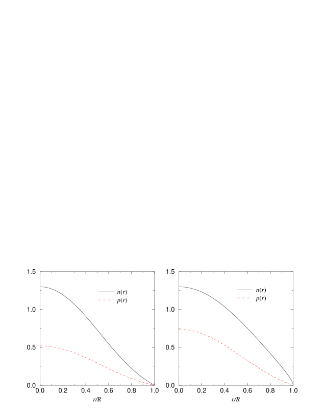
FIG. 2.: Number density profiles $n(r)$ and $p(r)$ for models one (left) and two (right) of Table I. $n$ and $p$ are given in units of ${\rm fm}^{-3}$.

FIG. 3.: Im($\omega M$) vs Re($\omega M$) for the w-modes for models one and two described in Table I, setting $l=2$.

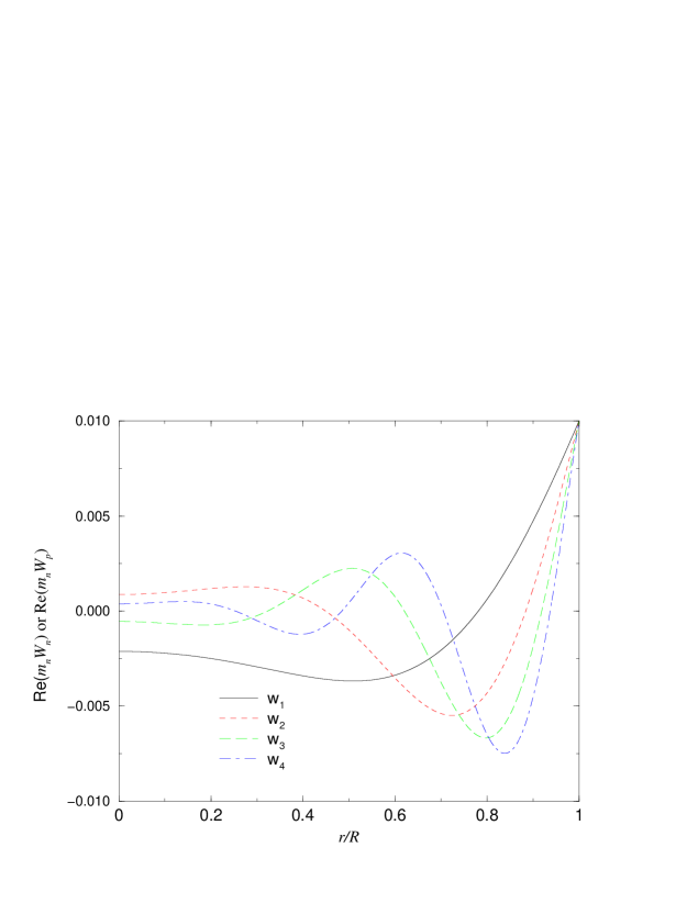
FIG. 4.: Re($m_{n}W_{n}$) or Re($m_{n}W_{p}$) (since they are indistinguishable) vs $r/R$ for the model one modes ${\rm w_{1}}$ through ${\rm w_{4}}$ listed in Table III.

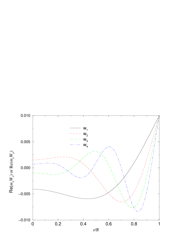
FIG. 5.: Re($m_{n}W_{n}$) or Re($m_{n}W_{p}$) (since they are indistinguishable) vs $r/R$ for the model two modes ${\rm w_{1}}$ through ${\rm w_{4}}$ listed in Table III.

FIG. 6.: ${\rm log}_{10}|A_{in}|$ vs ${\rm Re}(\omega M)$, with $l=2$, for model one of Table I, and for a one-fluid system composed of neutrons behaving as a relativistic polytrope (i.e. $\beta_{n}=\beta_{p}$, $\sigma_{n}=\sigma_{p}$, and with the same values for $n_{0}$, $\beta_{n}$, and $\sigma_{n}$ as model one).

FIG. 7.: ${\rm log}_{10}|A_{in}|$ vs ${\rm Re}(\omega M)$, with $l=2$, for model two of Table I, and for a one-fluid system composed of neutrons behaving as a relativistic polytrope (i.e. $\beta_{n}=\beta_{p}$, $\sigma_{n}=\sigma_{p}$, and with the same values for $n_{0}$, $\beta_{n}$, and $\sigma_{n}$ as model two).

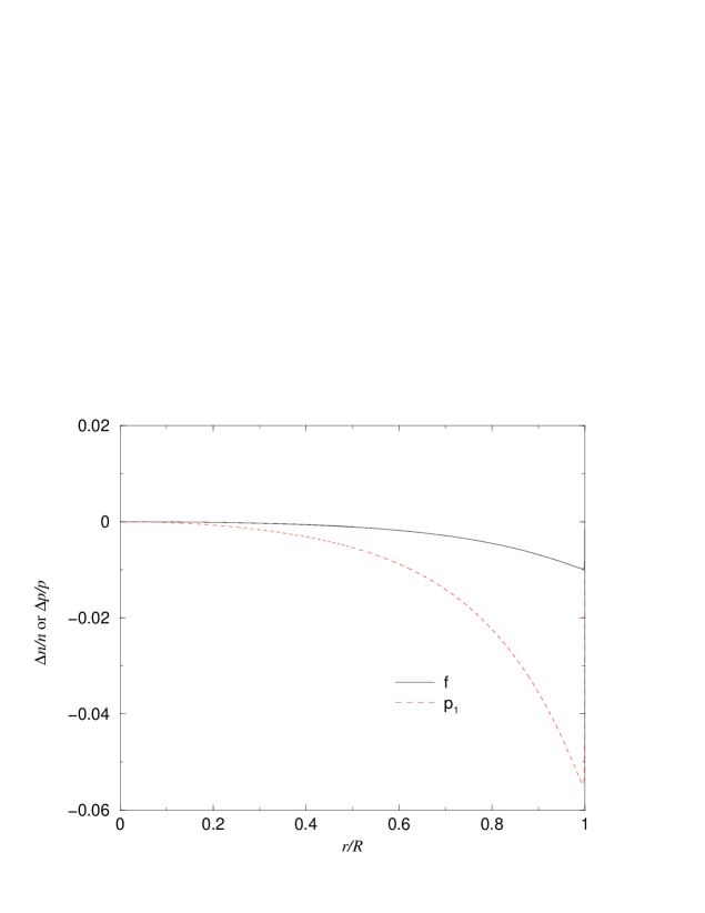
FIG. 8.: $\Delta n/n$ or $\Delta p/p$ (since they are indistinguishable) vs $r/R$, with $l=2$, for the model one f- and ${\rm p_{1}}$- modes listed in Table IV.

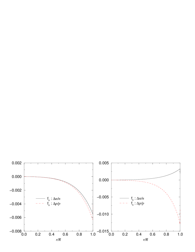
FIG. 9.: $\Delta n/n$ and $\Delta p/p$ vs $r/R$, with $l=2$, for the model two ${\rm f_{o}}$- and ${\rm f_{s}}$-modes listed in Table IV.

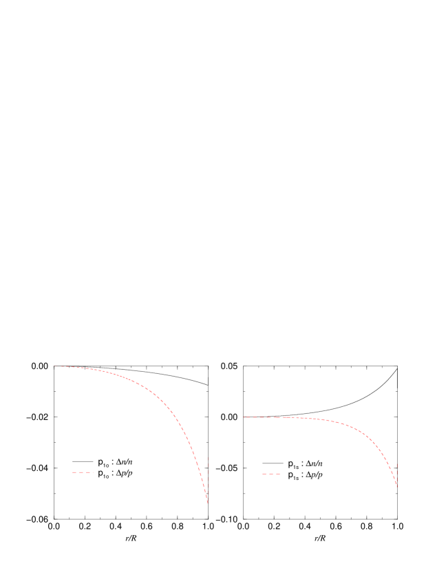
FIG. 10.: $\Delta n/n$ and $\Delta p/p$ vs $r/R$, with $l=2$, for the model two ${\rm p_{1o}}$- and ${\rm p_{1s}}$-modes listed in Table IV.

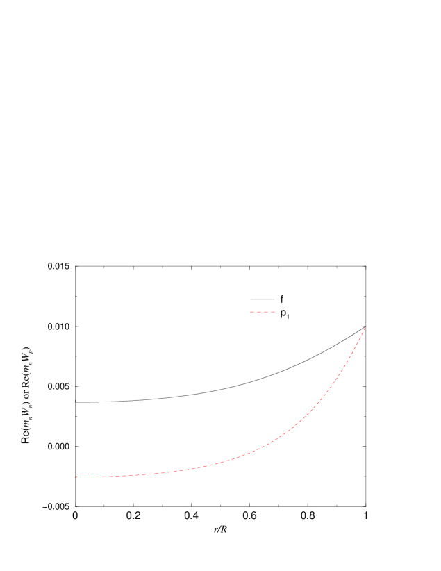
FIG. 11.: Re($m_{n}W_{n}$) or Re($m_{n}W_{p}$) (since they are indistinguishable) vs $r/R$, with $l=2$, for the model one f- and ${\rm p_{1}}$-modes listed in Table IV.

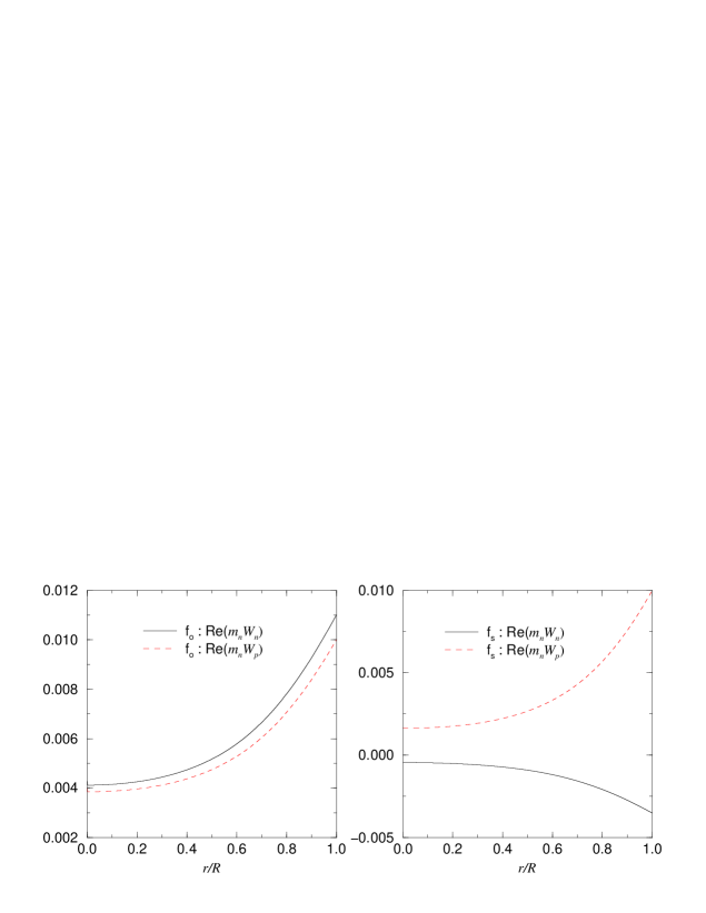
FIG. 12.: Re($m_{n}W_{n}$) and Re($m_{n}W_{p}$) vs $r/R$, with $l=2$, for the model two ${\rm f_{o}}$- and ${\rm f_{s}}$-modes listed in Table IV.

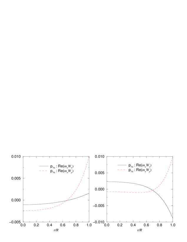
FIG. 13.: Re($m_{n}W_{n}$) and Re($m_{n}W_{p}$) vs $r/R$, with $l=2$, for the model two ${\rm p_{1o}}$- and ${\rm p_{1s}}$-modes listed in Table IV.

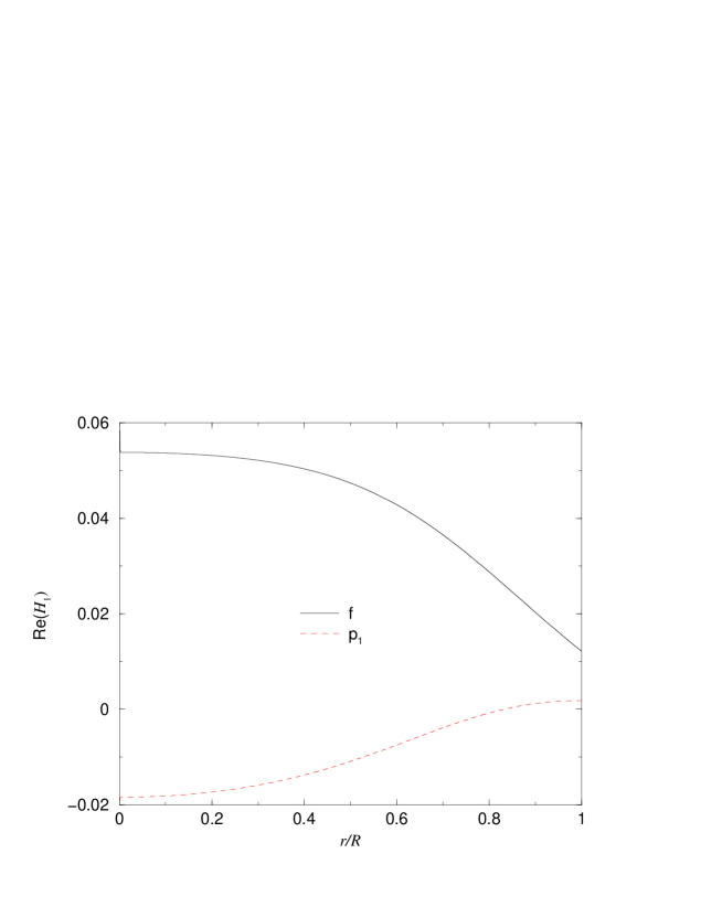
FIG. 14.: Re($H_{1}$) vs $r/R$, with $l=2$, for the model one f- and ${\rm p_{1}}$-modes listed in Table IV.

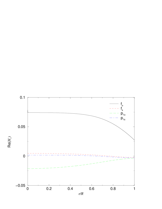
FIG. 15.: Re($H_{1}$) vs $r/R$, with $l=2$, for the model two ${\rm f_{o}}$-, ${\rm f_{s}}$-, ${\rm p_{1o}}$-, and ${\rm p_{1s}}$-modes listed in Table IV.

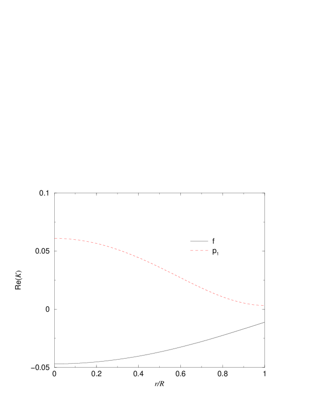
FIG. 16.: Re($K$) vs $r/R$, with $l=2$, for the model one f- and ${\rm p_{1}}$-modes listed in Table IV.

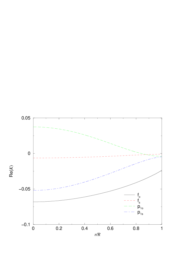
FIG. 17.: Re($K$) vs $r/R$, with $l=2$, for the model two ${\rm f_{o}}$-, ${\rm f_{s}}$-, ${\rm p_{1o}}$-, and ${\rm p_{1s}}$-modes listed in Table IV.

REFERENCES

- [1] A. B. Migdal, Nucl. Phys. 13, 655 (1959); J. Clark, R. Davé, and J. Chen, in The Structure and Evolution of Neutron Stars, D. Pines, R. Tamagaki, and S. Tsurate, eds. (Addison-Wesley, Redwood City, CA, 1992).
- [2] V. Radhakrishnan and R. N. Manchester, Nature, Lond. 244, 228 (1969); A. G. Lyne, in Pulsars as Physics Laboratories, R. D. Blandford, A. Hewish, A. G. Lyne, and L. Mestel, eds. (Oxford University Press Inc., New York, 1993).
- [3] S. Tsuruta, in The Lives of Neutron Stars, M. A. Alpar, U. Kiziloglu, and J. van Paradijs, eds. (Kluwer Academic Publishers, Dordrecht, 1995).
- [4] J. A. Sauls, in Timing neutron stars, H. B. Ogelman and E. P. J. van den Heuvel, eds. (Kluwer Academic Publishers, Dordrecht, 1988).
- [5] G. Mendell and L. Lindblom, Annals of Physics 205, 110 (1991).
- [6] G. Mendell, Ap. J. 380, 515 (1991); ibid, 530 (1991).
- [7] B. Carter and D. Langlois, Nucl. Phys. B 454, 402 (1998).
- [8] B. Carter and D. Langlois, Nucl. Phys. B 531, 478 (1998).
- [9] M. Alpar, S. A. Langer, and J. A. Sauls, Ap. J. 282, 533 (1984).
- [10] D. Langlois, A. Sedrakian, and B. Carter, Mon. Not. R. Astron. Soc. 297, 1189 (1998).
- [11] B. Carter and D. Langlois, Phys. Rev. D 51, 5855, 1995.
- [12] G. L. Comer and D. Langlois, Class. and Quant. Grav 11, 709 (1994).
- [13] S. J. Putterman, Superfluid Hydrodynamics (North-Holland, Amsterdam, 1974).
- [14] L. Lindblom and G. Mendell, Ap. J. 421, 689 (1994).
- [15] U. Lee, Astron. Astrophys. 303, 515 (1995).
- [16] S. L. Detweiller and L. Lindblom, Ap. J. 292, 12 (1985).
- [17] L. Lindblom and S. L. Detweiler, Ap. J. Supplement Series 53, 73 (1983).
- [18] S. Chandrasekhar, Ap. J. 140, 417 (1964).
- [19] K. S. Thorne and A. Campolattaro, Ap. J. 149, 591 (1967).
- [20] R. Price and K. S. Thorne, Ap. J. 155, 163 (1969).
- [21] K. S. Thorne, Ap. J. 158, 1 (1969).
- [22] K. S. Thorne, Ap. J. 158, 997 (1969).
- [23] A. Campolattaro and K. S. Thorne, Ap. J. 159, 847 (1970).
- [24] L. Lindblom and G. Mendell, Ap. J. 444, 804 (1995).
- [25] C. W. Misner, K. S. Thorne, and J. A. Wheeler, Gravitation (Freeman Press, San Francisco, 1973) pg. 608.
- [26] G. L. Comer and D. Langlois, Class. and Quant. Grav 10, 2317 (1993).
- [27] B. Carter, “Relativistic fluid dynamics”, A. Anile, M. Choquet-Bruhat, Eds, Springer-Verlag (1989).
- [28] T. Regge and J. A. Wheeler, Phys. Rev. 108, 1063 (1957).
- [29] F. J. Zerilli, Phys. Rev. D 2, 2141 (1970).
- [30] E. D. Fackerell, Ap. J. 166, 197 (1971).
- [31] D. R. Tilley and J. Tilley, Superfluidity and Superconductivity, 2nd Edition (Adam Hilger Ltd., Bristol, 1986), pg. 1.
- [32] E. W. Leaver, Proc. Roy. Soc. London A 402, 285 (1985).
- [33] E. W. Leaver, J. Math. Phys. 27, 1238 (1986).
- [34] Y. T. Liu, Master Thesis (unpublished), The Chinese University of Hong Kong (1997).
- [35] P. T. Leung, Y. T. Liu, W.-M. Suen, C. Y. Tam, and K. Young, Phys. Rev. D 59, 044034 (1999).
- [36] C. W. Yip, Master Thesis (unpublished), The Chinese University of Hong Kong (1998).
- [37] W. H. Press, S. A. Teukolsky, W. T. Vetterling, and B. P. Flannery, Numerical Recipes in FORTRAN, 2nd Edition (Cambridge University Press, New York, 1992), pg. 364.
- [38] K. D. Kokkotas and B. F. Schutz, Mon. Not. R. Astron. Soc. 268, 119 (1992).
- [39] N. Andersson, K. D. Kokkotas, and B. F. Schutz, Mon. Not. R. Astron. Soc. 280, 1230 (1996).
- [40] M. Leins, H. P. Nollert, and M. H. Soffel, Phys. Rev. D 48, 3467 (1993).
- [41] P. N. McDermott, H. M. Van Horn, and C. J. Hansen, Ap. J. 325, 725 (1988).
- [42] S. Chandrasekhar, The Mathematical Theory of Black Holes (Oxford University Press, New York, 1983), pgs. 160-163.