Symmetry without Symmetry: Numerical Simulation of
Axisymmetric Systems using Cartesian Grids

Abstract

We present a new technique for the numerical simulation of axisymmetric systems. This technique avoids the coordinate singularities which often arise when cylindrical or polar-spherical coordinate finite difference grids are used, particularly in simulating tensor partial differential equations like those of $3+1$ numerical relativity. For a system axisymmetric about the $z$ axis, the basic idea is to use a 3-dimensional Cartesian $(x,y,z)$ coordinate grid which covers (say) the $y=0$ plane, but is only one finite-difference-molecule–width thick in the $y$ direction. The field variables in the central $y=0$ grid plane can be updated using normal $(x,y,z)$–coordinate finite differencing, while those in the $y\neq 0$ grid planes can be computed from those in the central plane by using the axisymmetry assumption and interpolation. We demonstrate the effectiveness of the approach on a set of fully nonlinear test computations in $3+1$ numerical general relativity, involving both black holes and collapsing gravitational waves.

I Introduction

Finite difference numerical simulations of axisymmetric systems are most often, and most naturally, carried out in coordinate systems adapted to the symmetry of the underlying problem, e.g. polar spherical $(r,\theta,\phi)$ or cylindrical $(\rho,z,\phi)$ coordinates. However, the use of such coordinate systems brings with it delicate problems in finite differencing near the $z$ axis, particularly when tensor time-evolution partial differential equations (PDEs) are considered. Depending on the problem, it is often very difficult to obtain fully stable numerical evolutions near the axis, and for some problems it is difficult to even accurately discretize the equations there. Here we consider the problem for the Einstein equations of general relativity in axisymmetry, although our approach should be useful for other systems of PDEs (e.g. the Navier-Stokes equations), and also for the case of spherical symmetry.

There are several different types of $z$ axis difficulties, which depending on the physical system may occur singly or in combination. The simplest problem is that physically nonsingular terms in the equations may have indeterminate $0/0$ forms along the $z$ axis. Fortunately, such terms are generally easy to regularize by applying L’Hopital’s rule. For example, in polar spherical coordinates $(r,\theta,\phi)$, the flat-space Laplacian operator includes the term

$$\frac{1}{r^{2}\sin\theta}\,\partial_{\theta}\Big{(}\sin\theta\,\partial_{\theta}\Big{)}\,\,\text{.}$$ (1)

Assuming all fields to be smooth on the $z$ axis and applying L’Hopital’s rule, the $\theta\to 0$ limit of this term is easily seen to be

$$\frac{2}{r^{2}}\,\partial_{\theta\theta}\,\,\text{.}$$ (2)

However, even here there may be a problem with finite differencing: Although the $\theta\to 0$ limit of the term (1) is precisely (2), when we finite difference these terms the limiting relationship generally only holds in the limit where the grid spacing $\Delta\theta\to 0$. For any given (nonzero) $\Delta\theta$, the numerically computed values of (1) will have a $\theta\to 0$ limit which will in general differ somewhat from the numerical values of (2). This difference may give rise to finite differencing instabilities near the axis.

A more serious $z$ axis problem is that of $\infty-\infty$ cancellations, where a physically nonsingular quantity is computed as the sum of many terms, two or more of which are individually singular on the $z$ axis. For example, again using polar spherical coordinates, $(r,\theta,\phi)$, in the so-called “$3+1$” Einstein equations ([1]; see, for example, [2, 3] for general reviews), the 3-Ricci tensor component $R_{\theta\theta}$ is generically $O(1)$ on the $z$ axis, but it is computed as the sum of, among (many) other terms, $-{\textstyle\frac{1}{2}}g^{\phi\phi}\partial_{\theta\theta}g_{\phi\phi}$, which is generically $O(1/\theta^{2})$ near the $z$ axis. Although not impossible, regularizing terms of this nature is very difficult, requiring a detailed analysis of the generic behavior of the entire system of PDEs under consideration (for our example, the coupled $3+1$ evolution of Einstein’s equations, with constraint and coordinate equations) near the $z$ axis.

Collectively these problems can be very severe, crippling attempts to evolve systems with such symmetries (see, e.g. [4, 5, 6, 7]). Many solutions to the problems brought on by special coordinate systems have been attempted, including various regularization procedures [8, 9, 10, 11], Taylor expansions [10], the use of nonsingular-basis tensor components [6], spectral methods [12], and special coordinate conditions used to eliminate troublesome terms [4, 13, 5]. However, these methods tend to be complicated and not particularly robust.

On the other hand, 3D Cartesian coordinates contain no coordinate pathologies, and all terms in the equations governing the evolution of functions are typically completely regular, even at special points such as the origin or along a symmetry axis [14]. Normally, however, if one treats a spherical or axisymmetric system in 3D Cartesian coordinates one loses the ability to ignore irrelevant dimensions. For example, a spherically symmetric system should reduce to a 1D problem, depending only on the radius $r$, while an axisymmetric system reduces to a 2D problem, independent of the azimuthal coordinate $\phi$. In full 3D Cartesian coordinates, not only is the true symmetry of the problem potentially disturbed by the finite differences taken in a Cartesian coordinate system, but dimensional reductions do not occur, and the memory requirements are much larger, scaling as $N^{3}$, rather than as $N^{2}$ or $N$. For reasonable grid sizes of order hundreds of zones, these factors can become astronomical. In 3D numerical relativity, the problem is exacerbated by the need to carry a large number of 3D grid functions (typically over 100) in memory at all times. Some savings have been realized in cases where Cartesian coordinates are used for intrinsically axisymmetric or spherical problems by evolving only a single octant, reducing memory and computational requirements by a factor of eight, but this does not change the overall scaling with $N$.

Furthermore, while many problems are now treatable in 3D, where Cartesian coordinates are generally favored, testbeds for developing algorithms for the full 3D case are often carried out in lower dimensional cases, where the problems are simpler and where limiting solutions are known. However, working in special coordinate systems for lower dimensional test problems introduces difficulties specific to the coordinate system, and frequently techniques developed in special coordinate system do not carry over to the 3D Cartesian code. What is needed is a lower dimensional testbed that retains the same essential features present in the generic 3D case, at both the physical and computational level.

In this paper we describe a scheme which borrows from the singularity-free nature of full 3D Cartesian coordinates, and allows the treatment of axisymmetric and spherically symmetric problems without the memory constraints of full 3D Cartesian coordinates. Take the case of axisymmetry: The essential trick is to realize that in 3D Cartesian coordinates, an axisymmetric system can be computed in, say, the $x$-$z$ ($y=0$) plane alone. The $x$-$z$ system can be rotated about the $z$ axis to determine the solution at any $(x,y,z)$ point at a given instant of time. However, a 3D evolution also requires spatial derivatives in the $y$ direction, which (for non-scalar field variables) do not necessarily all vanish, even in the $x$-$z$ ($y=0$) plane. Because of the axisymmetry assumption, the solution in the $x$-$z$ ($y=0$) plane can be rotated according to tensor transformation laws to any $y$ value, so the $y$ derivatives of all quantities can be determined in the $x$-$z$ plane solely from information in this same plane. Hence, a full 3D evolution in Cartesian coordinates can be carried out, using only information from a single 2D plane of data. There are different ways to achieve this, as we show in the sections below, but the key point is that an axisymmetric or spherical system can be evolved as if it were in 3D Cartesian coordinates, and hence without coordinate singularities and the instabilities they can induce, and without going to the expense of a full 3D computation.

In section II we describe the technique in detail for the case of axisymmetry. We show the effectiveness of the method in applications to dynamic wave and black hole spacetimes in section III, and summarize the work in section IV. The method has been fully implemented under the name “Cartoon” (chosen because of its resemblance to the way low-budget television cartoons animate a nominally 3-dimensional world in “$2{\textstyle\frac{1}{2}}$” dimensions, and also as a shorthand for cartesian two-dimensional) in the Cactus code for numerical relativity and astrophysics [15, 16, 17, 18].

II The Technique

In 3D systems with discrete symmetries it has been common practice to evolve just a part of the domain, and use symmetries to provide boundary conditions. For example, spherical, axisymmetric, and even 3D systems have been evolved in numerical relativity in a single octant, if the symmetries of the system allow it. A spherical system is reflection symmetric about all coordinate planes, and hence it could be evolved in Cartesian coordinates in the octant defined by, say, $x,y,z$ all non-negative. Any planar reflection symmetry can be used to provide boundary conditions at the plane of reflection, i.e. from the symmetry one can infer that certain functions are either symmetric or antisymmetric across the coordinate planes. This has been used in many simulations in numerical relativity [17, 19, 20, 21, 22, 23, 24, 25, 26].

In what follows we discuss how in the case of axisymmetry one can use the continuous rotational symmetry to provide boundary conditions for a thin 3D slab. The same construction is expected to be applicable to spherically symmetric systems.

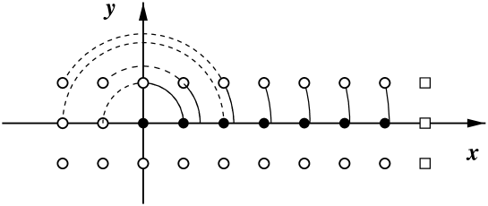
Consider a rectangular three dimensional volume in $R^{3}$, with Cartesian coordinates $(x,y,z)$. We assume a uniformly spaced Cartesian grid with spacings $\Delta x$, $\Delta y$, and $\Delta z$, and we take the finite difference molecules to have radii $v$ in the $x$ direction and $w$ in the $y$ direction. (For reasons discussed in section II B, we will typically have $v>w$.) We take the $z$ axis to be the axis of symmetry, as shown in Fig. 1. In the $y$ direction, the grid contains $2w+1$ points centered about $y=0$. (For example, for standard second order centered difference $w=1$, and there are points at $y=0$ and $\pm\,\Delta y$.) In the $x$ direction, the grid starts near the axis at $x_{\min}$ and extends out to some finite positive $x_{\max}$. We consider the two cases $x_{\min}=-(v-{\textstyle\frac{1}{2}})\Delta x$ (staggered) and $x_{\min}=-v\Delta x$ (non-staggered).

One can compute finite differences with a centered Cartesian 3D molecule in the interior plane of the slab, i.e. for all grid points at $x\geq 0$ and $y=0$, once boundary values are specified. The boundary values in the $z$ direction and the positive $x$ direction are assumed to be given as part of the general problem. As outlined above, the key point in the case of axisymmetry is that field values at points with $y\neq 0$, and also at the points with $x<0$, can be obtained through a rotation and interpolation from field values on the half plane $x\geq 0$ and $y=0$.

FIG. 1.: A typical numerical grid in a constant $z$ plane with $\Delta x=\Delta y$, no staggering, for a 3D molecule of radius 1. The arcs show the rotation allowed by axisymmetry to obtain various field values on the slab boundary (circles). High order interpolation in the $x$ direction may require several points at $x<0$; for these points the rotation is shown by dashed arcs. The outer boundary at $x_{\max}$ is given as part of the problem (squares). In the interior of the grid at $0\leq~{}x<x_{\max}$, $y=0$ (solid dots), the standard 3D finite difference stencil can be used.

A Rotation of Tensors

Let us first discuss the rotation of the tensors and non-tensors that arise in typical numerical relativity computations. The basic formula, Eq. (7) below, is (aside from a few subtleties in its derivation) precisely what one expects for a vector in $R^{3}$ in Cartesian coordinates. Consider the rotation of a tensor field by an angle $-\phi_{0}$ about the $z$ axis. Equivalently, we can view this as keeping the field fixed, but rotating the coordinates in the opposite direction, i.e. rotating them by $+\phi_{0}$. Taking this latter viewpoint, in cylindrical coordinates $(\rho,\phi,z)$ that are adapted to the rotation about the $z$ axis, the rotated coordinates are

$$\rho^{\prime}=\rho,\quad\phi^{\prime}=\phi+\phi_{0},\quad z^{\prime}=z,$$ (3)

or in the Cartesian coordinates given by $\rho=\sqrt{x^{2}+y^{2}}$, $\phi=\arctan(y/x)$,

$$x^{\prime}=x\cos\phi_{0}-y\sin\phi_{0},\quad y^{\prime}=x\sin\phi_{0}+y\cos\phi_{0},\quad z^{\prime}=z.$$ (4)

This coordinate transformation gives rise to the linear map

$$({R(\phi_{0})^{i}}_{j})=\left(\frac{\partial{x^{\prime}}^{i}}{\partial{x}^{j}}\right)=\left(\begin{array}[]{ccc}\cos\phi_{0}&-\sin\phi_{0}&0\\ \sin\phi_{0}&\cos\phi_{0}&0\\ 0&0&1\end{array}\right).$$ (5)

Note that $R(\phi_{0})^{-1}=R(-\phi_{0})$.

Now consider arbitrary tensor fields $T$ on a three-dimensional manifold $\Sigma$. Without referring to coordinates, a rotation (if it exists) defines a diffeomorphism $R:\Sigma\rightarrow\Sigma$, mapping points to points, and as such also defines a new tensor field $R^{*}T$ of the same contra- and covariant type as $T$. The diffeomorphism $R$ is a symmetry transformation for the tensor field $T$ if $R^{*}T=T$.

We assume, as is often the case in numerical relativity, that the domain of interest is covered by a single coordinate chart. The matrix of components of $R^{*}$ in the coordinate bases of the coordinate system $(x^{i})=(x,y,z)$ at a point $p$ and the coordinate system $(x^{\prime i})=(x^{\prime},y^{\prime},z^{\prime})$ at the point $R(p)$ equals the Jacobian matrix of the map $R$ between the coordinates, which is given in (5), if we assume coordinates adapted to the rotation. The components of a tensor $T$ at $p$, for example ${T^{i_{1},i_{2},\ldots}}_{j_{1},j_{2},\ldots}(p)$, transform according to

$${(R^{*}T)^{i_{1},i_{2},\ldots}}_{j_{1},j_{2},\ldots}(R(p))={R^{i_{1}}}_{k_{1}}{R^{i_{2}}}_{k_{2}}\ldots{(R^{-1})^{l_{1}}}_{j_{1}}{(R^{-1})^{l_{2}}}_{j_{2}}\ldots{T^{k_{1},k_{2},\ldots}}_{l_{1},l_{2},\ldots}(p).$$ (6)

In the case of axisymmetry ($R^{*}T=T$) we therefore arrive at

$${T^{i_{1},i_{2},\ldots}}_{j_{1},j_{2},\ldots}(x,y,z)={R^{i_{1}}}_{k_{1}}{R^{i_{2}}}_{k_{2}}\ldots{(R^{-1})^{l_{1}}}_{j_{1}}{(R^{-1})^{l_{2}}}_{j_{2}}\ldots{T^{k_{1},k_{2},\ldots}}_{l_{1},l_{2},\ldots}(\sqrt{x^{2}+y^{2}},0,z),$$ (7)

where $R$ is given by (5) with $\cos\phi_{0}=x/\rho$, $\sin\phi_{0}=y/\rho$, and $\rho=\sqrt{x^{2}+y^{2}}$. For example, for a vector $T^{i}$, $T^{i}(x,y,z)={R^{i}}_{j}T^{j}(\rho,0,z)$. Equation (7) describes how to compute the values of a tensor at points outside the half-plane $x\geq 0$ and $y\neq 0$ from points within this plane.

One type of non-tensor that is often used in numerical relativity is the partial derivative of tensors, $\partial_{k}{T^{i_{1},i_{2},\ldots}}_{j_{1},j_{2},\ldots}$. Under coordinate transformations, the index $k$ transforms by the chain rule of partial derivatives with the same Jacobian factor as appears in the coordinate transformation of a tensor, (6). Using (6) and the product rule, there appear additional terms containing $\partial_{k}{R^{i}}_{j}$. However, using coordinates that are adapted to the axisymmetry (5) implies $\partial_{k}{R^{i}}_{j}=0$ (in other words, $R$ describes a rigid rotation), and hence the basic transformation law (7) is also valid for partial derivatives of tensors in this context.

B 1D interpolation in the $x$ direction

We now turn to a brief discussion of the necessary interpolations. As made explicit in (7), we require fields at points $(\sqrt{x^{2}+y^{2}},0,z)$. As such points are not necessarily part of the numerical grid, a one-dimensional interpolation may be required. In this work we test Lagrange polynomial interpolation (e.g. [27, 28]) with interpolation polynomials of degrees 2 through 5, obtaining good results already with second order polynomials. Our evolution code uses second order finite difference molecules of size $v=w=1$, but for interpolation polynomials of degree larger than 2 we need $v>1$. Note that even the points at $x=x_{\max}$, $y\neq 0$ can be obtained through interpolation by first applying the physical boundary for $y=0$, then rotating to $y\neq 0$ for $x<x_{\max}$, and then applying the physical boundary at $x=x_{\max}$, $y\neq 0$.

This sort of interpolation is used in many areas of computational science (e.g. in adaptive mesh refinement), and thus should not be expected to pose a serious threat to the success of this technique. The principal issue of concern is whether interpolation might destabilize an evolution scheme that often is carefully crafted using particular forms of centered stencils and averages. This must be addressed on a case-by-case basis, either by Von Neumann or other analytical stability analysis, and/or by numerical experiment.

Although we do not do it in practice, instead of explicitly computing and storing field values at the boundaries in the $y$ direction, one can make the polynomial interpolation a part of the stencil, thereby explicitly reducing the 3D stencil to an inhomogeneous and asymmetric – but nonsingular – 2D stencil. In contrast, storing field values for a 3D stencil allows us to simply use numerical routines from existing Cartesian 3D codes.

III Applications

In this section we provide two important tests, both with the complete set of 3D, nonlinear Einstein evolution equations, performed with “Cartoon” in the Cactus code for numerical relativity [15, 16, 17, 18]. However, we stress that the techniques developed here are applicable to many families of partial differential equations. That our tests are so successful, with such a complicated set of tensor PDEs as the $3+1$ Einstein equations involving dozens of coupled nonlinear evolution equations, stresses this point. Simpler sets of equations can be expected to have fewer complications: less severe regularity issues at symmetry points (origin or axis), simpler transformation laws in the rotation to provide boundary conditions, etc.

A Einstein’s Equations

In this section we give a brief introduction to the basic equations we will be solving. The Einstein equations of general relativity in 3+1 form (see [2, 3] for recent reviews and further references) are a complicated set of coupled, nonlinear partial differential equations for the symmetric tensor fields $\gamma_{ij}$ and $K_{ij}$ (indices range from $1$ through $3$, so there are 12 field variables in all). The metric $\gamma_{ij}$ is the spatial part of the spacetime metric (which gives the invariant distance between two infinitesimally separated events):

$$ds^{2}=-(\alpha^{2}-\beta^{i}\beta_{i})\,dt^{2}+2\beta_{i}\,dx^{i}dt+\gamma_{ij}\,dx^{i}dx^{j}.$$ (8)

The extrinsic curvature, $K_{ij}$, specifies how the $t={\text{constant}}$ slices are embedded in spacetime. The equations also involve the auxiliary tensor fields $\alpha$ and $\beta^{i}$. These so-called “gauge” fields carry no dynamical information: they may be freely chosen for convenience. The lapse function $\alpha$ determines the proper time $d\tau=\alpha\,dt$ measured by an observer falling normal to the time slice defined by $t={\text{constant}}$. The shift vector $\beta^{i}$ determines the coordinate distance a constant-coordinate point moves away from the normal vector to the slice as one advances from one slice to the next. In the tests performed in this paper, we choose $\beta^{i}=0$ for simplicity.

The evolution equations can be written as:

$$\partial_{t}\gamma_{ij}=-2\alpha K_{ij}+D_{i}\beta_{j}+D_{j}\beta_{i},$$ (10)

$$\partial_{t}K_{ij}= -D_{i}D_{j}\alpha+\alpha[R_{ij}+(\mathop{\rm tr}\nolimits K)K_{ij}-2K_{ik}K^{k}{}_{j}]$$ (12)

$$+\beta^{k}D_{k}K_{ij}+K_{ik}D_{j}\beta^{k}+K_{jk}D_{i}\beta^{k}.$$

In these equations $R_{ij}$ is the 3-Ricci tensor, $R$ is the 3-scalar curvature (both nonlinear functions of the metric $\gamma_{ij}$ and its first and second spatial derivatives), $\mathop{\rm tr}\nolimits K$ is the trace of $K_{ij}$, and $D_{i}$ is the covariant derivative associated with the 3-metric $\gamma_{ij}$. With suitable choices for $\alpha$ and $\beta^{i}$, equations (III A) are hyperbolic in $\gamma_{ij}$ and $K_{ij}$.

The fields $\gamma_{ij}$ and $K_{ij}$ are not completely freely specifiable: on each $t={\text{constant}}$ slice they must satisfy the four constraint equations

$$H\equiv R+(\mathop{\rm tr}\nolimits K)^{2}-K_{ij}K^{ij}=0,$$ (14)

$$H^{i}\equiv D_{j}(K^{ij}-g^{ij}\mathop{\rm tr}\nolimits K)=0,$$ (15)

where for later use we define the left hand side functions as $H$ (known as the Hamiltonian constraint) and $H^{i}$. Eqs. (III A) are elliptic equations in $\gamma_{ij}$ and $K_{ij}$; in general they must be solved numerically in order to obtain valid initial data ([29]). However, one can show that once the constraints are satisfied on an initial slice, they are preserved by the evolution equation (III A) (i.e. they stay satisfied for all future times). This statement holds for the continuum equations (III A) and (III A); a finite difference evolution will in general only approximately satisfy the constraints at later times ([30]), and in fact the deviations of $H$ and $H^{i}$ from zero are useful diagnostics of the evolution’s numerical accuracy.

To understand the physical meaning of these equations it is useful to consider an analogy with Maxwell’s equations in a vacuum: $\gamma_{ij}$ and $K_{ij}$ are analogous to the (vector) electric and magnetic fields $\textstyle E$ and $\textstyle B$, the evolution equations (III A) are analogous to the Maxwell equations $\partial_{t}\mathchoice{{\hbox{\boldmath$\displaystyle E$}}}{{\hbox{\boldmath$\textstyle E$}}}{{\hbox{\boldmath$\scriptstyle E$}}}{{\hbox{\boldmath$\scriptscriptstyle E$}}}=\nabla\times\mathchoice{{\hbox{\boldmath$\displaystyle B$}}}{{\hbox{\boldmath$\textstyle B$}}}{{\hbox{\boldmath$\scriptstyle B$}}}{{\hbox{\boldmath$\scriptscriptstyle B$}}}$ and $\partial_{t}B=-\nabla\times\mathchoice{{\hbox{\boldmath$\displaystyle E$}}}{{\hbox{\boldmath$\textstyle E$}}}{{\hbox{\boldmath$\scriptstyle E$}}}{{\hbox{\boldmath$\scriptscriptstyle E$}}}$, and the constraint equations (III A) are analogous to the Maxwell equations $\nabla\cdot\mathchoice{{\hbox{\boldmath$\displaystyle E$}}}{{\hbox{\boldmath$\textstyle E$}}}{{\hbox{\boldmath$\scriptstyle E$}}}{{\hbox{\boldmath$\scriptscriptstyle E$}}}=\nabla\cdot\mathchoice{{\hbox{\boldmath$\displaystyle B$}}}{{\hbox{\boldmath$\textstyle B$}}}{{\hbox{\boldmath$\scriptstyle B$}}}{{\hbox{\boldmath$\scriptscriptstyle B$}}}=0$, with $H$ and $H^{i}$ analogous to $\nabla\cdot\mathchoice{{\hbox{\boldmath$\displaystyle E$}}}{{\hbox{\boldmath$\textstyle E$}}}{{\hbox{\boldmath$\scriptstyle E$}}}{{\hbox{\boldmath$\scriptscriptstyle E$}}}$ and $\nabla\cdot\mathchoice{{\hbox{\boldmath$\displaystyle B$}}}{{\hbox{\boldmath$\textstyle B$}}}{{\hbox{\boldmath$\scriptstyle B$}}}{{\hbox{\boldmath$\scriptscriptstyle B$}}}$. However, unlike Maxwell’s equations, the Einstein equations are nonlinear, quite complicated (they have on the order of 1000 terms when written out in scalar form in terms of coordinate partial derivatives), and second order in space (though still first order in time). These properties make the Einstein equations difficult to treat numerically.

As the main point of our paper is a technique for solving any set of evolution equations, we simply state that the particular form of the equations we use for this paper is a variant of (III A) and (III A) recently put forth by Baumgarte and Shapiro [31], based on previous work of Shibata and Nakamura [32]. We will refer to this as the BSSN formulation. It is to be noted that this formulation is quite similar in many respects to the Bona-Massó formulation [33, 34, 35]. In another paper [36] we detail experiments carried out with these formulations on various spacetimes. As these details are not important to the results presented here, in this paper we focus only on the technique and its application to a very general class of partial differential equations, as represented by the Einstein equations.

B Black hole spacetimes

In this section we report on the application of the Cartoon technique to the nonlinear evolution of black holes in the strong field regime. To illustrate the power of this technique, we focus on the case of a Schwarzschild black hole evolved with geodesic slicing. Geodesically sliced black hole evolutions have been used extensively to test black hole codes in 1D [37] and 2D [5, 22] in polar-spherical type coordinates, and in 3D Cartesian coordinates [19, 21, 22, 24]. This black hole case has the advantages of (i) having an analytic and also a highly accurate numerical 1D solution; (ii) providing a demanding test, as the slicing rapidly approaches the spacetime singularity, and hence spacetime curvature and metric functions grow rapidly and without bound until the code crashes at time $t=\pi M$, where $M$ is the mass of the black hole; (iii) being one of the simpler testbeds in strong field regimes, as the geodesic slicing condition ($\alpha=1$) does not involve coupling additional elliptic or parabolic equations, which could complicate the demonstration of the technique. In the following section we consider a more complex system as a further test of the Cartoon method.

The initial 3-metric for the Schwarzschild black hole is given by

$$ds^{2}=\psi^{4}(dr^{2}+r^{2}(d\theta^{2}+\sin^{2}\theta d\phi^{2})),$$ (16)

where the conformal factor is $\psi=(1+\frac{M}{2r})$. Here $r$ is the isotropic radius, related to the standard Schwarzschild radius $r_{s}$ by $r_{s}=(1+\frac{M}{2r})^{2}r$. Transforming to Cartesian coordinates, we have

$$ds^{2}=\psi^{4}(dx^{2}+dy^{2}+dz^{2}),$$ (17)

where the Cartesian coordinates $x$, $y$, and $z$ are related to the isotropic radius $r$ in the usual way. The extrinsic curvature for the time symmetric, $t=0$ slice of this spacetime vanishes.

We evolve this black hole in Cartesian coordinates, using the Cartoon technique. While typical 3D simulations of the Einstein equations are currently limited to grid sizes of roughly $100^{3}$ (ignoring the possibility of mesh refinements [38]), and the largest production simulations are currently at around $300^{3}-400^{3}$ [25, 39] on a 128Gbyte SGI/Cray Origin 2000 supercomputer with 256 processors, in this simulation we compute the evolution on a grid of $N_{x}\times N_{y}\times N_{z}=1025\times 3\times 2049$. (Our current implementation of the technique requires the $z$ direction to range from $+z_{\max}$ to $-z_{\max}$.) This is equivalent to a full 3D calculation of $2049^{3}$, over two orders of magnitude larger than the largest production simulations to date. Yet with this technique, the calculation requires only 0.07% of the memory required to do the full 3D simulation, and was run on 8 processors of an Origin 2000 over a period of 40 hours.

In more detail, the present calculation was performed for a unit mass black hole, with $\Delta x=\Delta y=\Delta z=0.01$, utilizing an iterative-Crank-Nicholson (ICN) method of lines evolution scheme with three iterations, a time step $\Delta t=0.1,spatialgridresolution\Delta x=0.001$, and 4th order Lagrange polynomial interpolation for the Cartoon algorithm. The total number of time steps for such a simulation was 3000 (9000 ICN iterations), corresponding to a time of $t=3.0$.

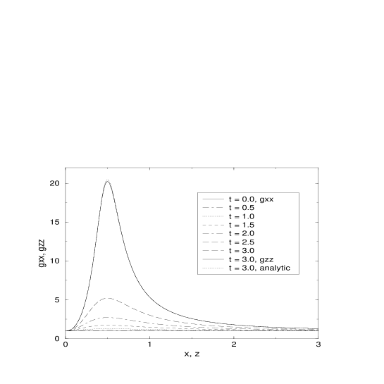
In Fig. 2 we show the metric function $g_{xx}$ on the $x$ axis at selected times during the evolution. There is no hint of any instability in the result. At $t=3.0$, a rather small difference between the numeric and analytic result (cmp. [21, 17]) can be seen at the peak of $g_{xx}$. At $t=3.0$ we also show $g_{zz}$ on the $z$ axis, which at this scale is indistinguishable from the numerical $g_{xx}$ on the $x$ axis, as it should be for this spherically symmetric data. The $z$ direction is computed quite differently from the $x$ direction, and suffers from the maximal inhomogeneity of the Cartoon stencil due to the interpolation near the $z$ axis. Yet results along the $z$-axis remain accurate and stable until the end of the simulation, giving a strong indication of the robustness of the technique.

FIG. 2.: We show results for a geodesically sliced Schwarzschild black hole, evolved in 3D with the Cartoon technique. The metric function $g_{xx}$ is shown on the $x$ axis at times $t/M=0.0,0.5,\ldots,3.0$, where $M$ is the mass of the black hole. At $t/M=3.0$, $g_{zz}$ on the $z$ axis is also plotted, but it is indistinguishable from $g_{xx}$ as expected for spherical symmetry. Both agree well with the analytic result.

In Fig. 3 we demonstrate second order convergence of the Cartoon evolution. We use the Hamiltonian constraint $H$ as a diagnostic of the evolution’s numerical accuracy: since $H$ vanishes analytically, it should converge to zero as the grid resolution increases. In particular, for second order finite differencing, each time the grid resolution is doubled $H$ should shrink by a factor of 4 ([30]). The figure shows the maximum value of $H$ in the grid as a function of time, plotted for the 3 different grid resolutions $\Delta x=\Delta y=\Delta z=0.02,0.04,0.08$, with each successive plot divided by $1,4,16$ respectively, so the values should be identical at the different resolutions. Second order convergence is directly evident from the figure.

FIG. 3.: The maximum of the Hamiltonian constraint for a geodesically sliced black hole at three different resolutions. Each graph is scaled proportionally to the inverse square of the grid resolution. The equality of the rescaled values for the different resolutions indicates second order convergence.

It is to be noted that not only is such a simulation impossible today in full 3D due to memory constraints, but the 2D Cartoon run has far higher resolution than has been achieved even in 2D codes designed to treat similar problems. Axisymmetric simulations of black holes, usually performed in spherical-polar coordinates, are typically not performed with more than 300 radial and 50 angular zones [40, 41, 7, 42]. Inherent axis instabilities usually create difficulties in simulations with higher resolution than this, in part because angular zones closer to the axis have more delicate regularity behavior to enforce. It is precisely these sorts of problems Cartoon is designed to overcome.

The problem with standard axisymmetric codes are exacerbated unless certain gauges are used that force troublesome terms in the three–metric to vanish. For example, as discussed in Ref. [5], a vicious axis instability arose in simulations of spherical or distorted black holes in axisymmetry, causing a rapid code crash, until a gauge condition was developed that diagonalized the three–metric. This condition required the solution of an elliptic equation to determine $\beta^{i}$ at each time step, which is very time consuming to solve numerically. Furthermore, even with this gauge choice, if the code is run with too high a resolution, axis instabilities are again encountered, and these instabilities eventually crash the code at late times. Similar problems with axis instabilities have been encountered in the case of rotating [6, 43, 40, 41] and colliding black holes [44, 4, 45, 46, 7, 42, 47].

As reported recently in Ref. [24], a case similar to the one presented here, a geodesically sliced perturbed black hole, was studied to compare results from a 3D code in Cartesian coordinates to a traditional 2D axisymmetric code. In order to compare metric functions directly, the codes had to be run with the same spatial gauge, which had vanishing shift. Although the agreement was excellent for as long as it could be computed, due to the axis instability the axisymmetric code crashed far earlier than the time at which the slice hit the singularity. On the other hand, the 3D Cartesian code, due to its lack of coordinate singularities, was able to run accurately all the way to the singularity. With our Cartoon technique, we are able to do the same simulation in Cartesian coordinates, with the same accuracy and stability, but with far less memory than is required in full 3D, and with far more stability than is possible in a standard axisymmetric code.

C Gravitational wave spacetimes

While the above simulation of time slices approaching a black hole singularity provide a strong test of the techniques we have developed, the underlying system is spherically symmetric, and does not contain gravitational waves. In order to further test and confirm this technique, we now turn to a completely different spacetime system, one not initially containing no black hole. Instead, the system we choose is that of highly nonlinear gravitational waves.

Gravitational waves are often considered in the linearized regime, where they are small disturbances on some background (often flat) spacetime that propagate at the speed of light. However, as the Einstein equations are nonlinear, for cases where the waves have sufficiently large amplitude they can affect the background spacetime on which they propagate. Even more, for strong enough waves there is no background spacetime; the waves have to be treated fully nonlinearly, and under extreme conditions they can even collapse in on themselves, forming a black hole when none existed previously.

Low amplitude gravitational waves have provided testbeds of 3D numerical relativity codes for the last decade, and even there they have provided a strong challenge [32, 20, 17]. Extreme gravitational wave simulations, where the waves form their own background, and where they may actually form black holes, have only been possible to evolve in full 3D codes during the last year [48]. For waves above a certain critical amplitude a black hole forms, while for waves just below critical a rich pattern of oscillations develops as the waves teeter on the edge of forming a black hole, and then eventually they disperse and the system returns to flat space (in a highly nontrivial coordinate system).

In this paper we use one such simulation to illustrate the strength of the Cartoon technique, and compare with a full 3D simulation as a measure of its accuracy. As our main purpose here is to demonstrate that the technique is robust, even under very demanding simulations, we will not go into detail of the physics of these simulations. The interested reader is asked to consult Ref. [48] for more details.

As in Ref. [48], we take as initial data a pure gravitational wave data set, based on the axisymmetric ansatz of Brill [49], and later studied by Eppley [45, 50, 51] and others [52, 53]. The metric takes the form

$$ds^{2}=\Psi^{4}\left[e^{2q}\left(d\rho^{2}+dz^{2}\right)+\rho^{2}d\phi^{2}\right]=\Psi^{4}\hat{ds}^{2},$$ (18)

where $q$ is a free function subject to certain boundary conditions. We consider a function $q$ of the form

$$q=a\;\rho^{2}\;e^{-r^{2}},$$ (19)

where $a$ is a constants, and $r^{2}\equiv\rho^{2}+z^{2}$ (see [52] for 2D, and [54, 48] for full 3D Cartesian coordinates). We consider data with the amplitude $a=4$ which corresponds to a strong, axisymmetric, equatorial plane symmetric gravitational wave. We choose the extrinsic curvature to vanish (time symmetric initial data). As shown in Ref. [48], this initial data collapses in on itself initially, but after a series of reverberations it disperses, leaving flat space in its wake.

Taking this form for $q$, we solve the Hamiltonian constraint equation (14) numerically using a multigrid elliptic solver on an $N_{x}\times N_{y}\times N_{z}=(129\times 3\times 257)$ grid, with $\Delta x=\Delta y=\Delta z=0.04$, and the outer boundary at $5.12$. As this axisymmetric initial data set is also symmetric about all coordinate planes, it is possible to evolve it as a full 3D system in just one octant ($x,y,z$ non-negative), as was also done in Ref. [48]. The same system is solved numerically in full 3D (with octant symmetry) on an $N_{x}\times N_{y}\times N_{z}=(129\times 129\times 129)$ grid, again with $\Delta x=\Delta y=\Delta z=0.04$, as a comparison simulation.

Both the full 3D system and the slab system were evolved to a time when the gravitational waves had largely left the system (through outgoing boundary conditions applied on the evolved function; see Ref. [48] for details). In Fig. 4, as a sensitive measure of the evolution we show the minimum value of the lapse function $\alpha$ as a function of time throughout the evolution. We have found this to be a good indicator of the evolution of the system [48], and also, as it sits on the axis and origin of the system, it should be especially sensitive to any problems that arise during the evolution due to the Cartoon procedure. We show results for 3D, and for Cartoon using interpolation of order 2, 3, and 4. The agreement is excellent. There is a discernible difference between the 3D and Cartoon runs after time $t=10$, starting with a slight bump that can be seen in the slab evolution that is not present in the full 3D simulation. This is due to slight differences in the boundary treatment in the two cases. There is no known perfect outgoing wave condition for general relativity (nor even a clear way to identify what a wave is in a nonlinear situation such as this), and small differences in boundary treatment can lead to differing amounts of reflection at the boundaries. The different geometries of the two simulations lead to different characteristics of the boundary treatment, which are ultimately reflected in the results. The origin of this difference is well-understood, to be expected, and minor, and is unrelated to the main thrust of this paper.

FIG. 4.: The minimum of the lapse during the evolution of a strong Brill wave, which generically occurs at the origin and is a sensitive measure of the spacetime evolution. We compare three Cartoon runs using interpolation order 2, 3, and 4, with a 3D run.

IV Conclusions

We have developed a novel technique for computational simulations with certain symmetries. This Cartoon technique allows simulations to be performed in 3D Cartesian coordinates, thereby avoiding difficulties associated with coordinate singularities that often lead to numerical instabilities. Compared to the full 3D Cartesian approach, Cartoon allows a huge savings in both memory and computational time, without introducing problems commonly associated with the singular coordinate systems which are usually employed. The Cartoon technique should be useful for any system of partial differential equations, and we have shown that it works well in one of the most complicated sets of equations in theoretical physics, Einstein’s equations of general relativity.

While this approach to axisymmetric simulation inherits many of the advantages of 3D Cartesian simulations, there are also some disadvantages which carry over. For example, a 2D code using angular coordinates can align spherical boundaries at constant coordinate value. Furthermore, a logarithmic or other stretched radial coordinate can be introduced that significantly improves resolution for problems with asymptotic $1/r$ fall-off. Even though neither of these techniques are readily incorporated in the Cartoon method, we nonetheless expect Cartoon to have a great impact on numerical relativity, as general purpose stable 2D codes are not currently available in the field.

Furthermore, as most fully 3D simulations are carried out in the same Cartesian coordinates as are found in Cartoon, experience gained from the accelerated Cartoon simulations should carry over directly to the full 3D work. This has generally not been the case previously, as special coordinate systems used for axisymmetric or spherically symmetric systems also required special treatments and gauge conditions that simply were not applicable in 3D Cartesian coordinates. Hence with our new technique systems can be studied with the same coordinate systems, with the same gauges, and with the same analysis tools as they will be when performed in full 3D. Finally, this technique has the potential to allow for a number of intrinsically axisymmetric systems to be studied with unprecedented stability and accuracy, since simulations with resolutions of several thousand grid points on a side are readily achievable.

We have implemented this technique in the Cactus code for 3D numerical relativity and the Cactus Computational Toolkit, and we expect that it will be a powerful addition to the field of numerical relativity.

Acknowledgments. The basic idea for this work was suggested by Steven Brandt. Special thanks are due to Paul Walker for early input on this idea. This work was supported by the AEI, NSF PHY 98-00973, and FWF P12754-PHY. The calculations were performed at the AEI. We thank many colleagues at the AEI, NCSA, Univeristat de les Illes Balears, and Washington University for the co-development of the Cactus code.

REFERENCES

- [1] R. Arnowitt, S. Deser, and C. W. Misner, in Gravitation: An Introduction to Current Research, edited by L. Witten (John Wiley, New York, 1962), pp. 227–265.
- [2] J. York, in Sources of Gravitational Radiation, edited by L. Smarr (Cambridge University Press, Cambridge, England, 1979).
- [3] J. York, in Gravitational Radiation, edited by N. Deruelle and T. Piran (North-Holland, Amsterdam, 1983), pp. 175–201.
- [4] L. Smarr, Ph.D. thesis, University of Texas, Austin, Austin, Texas, 1975.
- [5] D. Bernstein et al., Phys. Rev. D 50, 5000 (1994).
- [6] J. Thornburg, Ph.D. thesis, University of British Columbia, Vancouver, British Columbia, 1993.
- [7] P. Anninos et al., Technical Report No. 24, National Center for Supercomputing Applications (unpublished).
- [8] C. Evans, in Dynamical Spacetimes and Numerical Relativity, edited by J. Centrella (Cambridge University Press, Cambridge, England, 1986), pp. 3–39.
- [9] R. Stark, in a talk given in Austin, TX, October 1991 (unpublished).
- [10] E. Seidel, Ph.D. thesis, Yale University, 1988.
- [11] E. Seidel, Phys. Rev. D 42, 1884 (1990).
- [12] S. Bonazzola and J.-A. Marck, in Frontiers in Numerical Relativity, edited by C. Evans, L. Finn, and D. Hobill (Cambridge University Press, Cambridge, England, 1989), pp. 239–253.
- [13] D. Bernstein, Ph.D. thesis, University of Illinois Urbana-Champaign, 1993.
- [14] J. M. Bardeen and T. Piran, Phys. Reports 196, 205 (1983).
- [15] http://cactus.aei-potsdam.mpg.de.
- [16] G. Allen, T. Goodale, and E. Seidel, in 7th Symposium on the Frontiers of Massively Parallel Computation-Frontiers 99 (IEEE, New York, 1999).
- [17] C. Bona, J. Massó, E. Seidel, and P. Walker, (1998), gr-qc/9804065, submitted to Phys. Rev. D.
- [18] E. Seidel and W.-M. Suen, J. Comp. Appl. Math. (1999), in press.
- [19] P. Anninos et al., Phys. Rev. D 52, 2059 (1995).
- [20] P. Anninos et al., Phys. Rev. D 56, 842 (1997).
- [21] B. Brügmann, Phys. Rev. D 54, 7361 (1996).
- [22] K. Camarda, Ph.D. thesis, University of Illinois at Urbana-Champaign, Urbana, Illinois, 1998.
- [23] K. Camarda and E. Seidel, Phys. Rev. D 57, R3204 (1998), gr-qc/9709075.
- [24] K. Camarda and E. Seidel, Phys. Rev. D 59, 064026 (1999), gr-qc/9805099.
- [25] G. Allen, K. Camarda, and E. Seidel, (1998), gr-qc/9806036, submitted to Phys. Rev. D.
- [26] G. Allen, K. Camarda, and E. Seidel, (1998), in preparation.
- [27] G. E. Forsythe, M. A. Malcolm, and C. B. Moler, Computer Methods for Mathematical Computations (Prentice-Hall, Englewood Cliffs, 1977).
- [28] W. H. Press, B. P. Flannery, S. A. Teukolsky, and W. T. Vetterling, Numerical Recipes (Cambridge University Press, Cambridge, England, 1986).
- [29] J. W. York, Jr. and T. Piran, in Spacetime and Geometry: The Alfred Schild Lectures, edited by R. A. Matzner and L. C. Shepley (University of Texas Press, Austin (Texas), 1982), pp. 147–176.
- [30] M. Choptuik, Phys. Rev. D 44, 3124 (1991).
- [31] T. W. Baumgarte and S. L. Shapiro, Physical Review D 59, 024007 (1999).
- [32] M. Shibata and T. Nakamura, Phys. Rev. D 52, 5428 (1995).
- [33] C. Bona and J. Massó, Phys. Rev. Lett. 68, 1097 (1992).
- [34] C. Bona, J. Massó, and J. Stela, Phys. Rev. D 51, 1639 (1995).
- [35] C. Bona, J. Massó, E. Seidel, and J. Stela, Phys. Rev. D 56, 3405 (1997).
- [36] M. Alcubierre et al., in preparation (1999).
- [37] D. Bernstein, D. Hobill, and L. Smarr, in Frontiers in Numerical Relativity, edited by C. Evans, L. Finn, and D. Hobill (Cambridge University Press, Cambridge, England, 1989), pp. 57–73.
- [38] B. Brügmann, Int. J. Mod. Phys. D 8, 85 (1999).
- [39] E. Seidel, in Proceedings of the Yukawa Conference (Kyoto, Japan, 1999).
- [40] S. Brandt and E. Seidel, Phys. Rev. D 52, 856 (1995).
- [41] S. Brandt and E. Seidel, Phys. Rev. D 52, 870 (1995).
- [42] P. Anninos et al., Phys. Rev. D 52, 2044 (1995).
- [43] S. Brandt and E. Seidel, Phys. Rev. D 54, 1403 (1996).
- [44] A. Čadež, Ph.D. thesis, University of North Carolina at Chapel Hill, Chapel Hill, North Carolina, 1971.
- [45] K. Eppley, Ph.D. thesis, Princeton University, Princeton, New Jersey, 1975.
- [46] L. Smarr, in Sources of Gravitational Radiation, edited by L. Smarr (Cambridge University Press, Cambridge, England, 1979), p. 245.
- [47] P. Anninos, S. R. Brandt, and P. Walker, Phys. Rev. D 57, (1997), gr-qc/9712047.
- [48] M. Alcubierre et al., (1999), gr-qc/9904013.
- [49] D. Brill and R. Lindquist, Phys. Rev. 131, 471 (1963).
- [50] K. Eppley, Phys. Rev. D 16, 1609 (1977).
- [51] K. Eppley, in Sources of Gravitational Radiation, edited by L. Smarr (Cambridge University Press, Cambridge, England, 1979), p. 275.
- [52] D. Holz, W. Miller, M. Wakano, and J. Wheeler, in Directions in General Relativity: Proceedings of the 1993 International Symposium, Maryland; Papers in honor of Dieter Brill, edited by B. Hu and T. Jacobson (Cambridge University Press, Cambridge, England, 1993).
- [53] A. Gentle, D. Holz, W. Miller, and J. Wheeler, Class. Quant. Grav. 16, 1979 (1999), gr-qc/9812057.
- [54] M. Alcubierre et al., (1998), gr-qc/9809004.