String excitation inside generic black holes

Abstract

We calculate how much a first-quantized string is excited after crossing the inner horizon of charged Vaidya solutions, as a simple model of generic black holes. To quantize a string suitably, we first show that the metric is approximated by a plane-wave metric near the inner horizon when the surface gravity of the horizon $\kappa_{I}$ is small enough. Next, it is analytically shown that the string crossing the inner horizon is excited infinitely in an asymptotically flat spacetime, while it is finite in an asymptotically de Sitter spacetime and the string can pass across the inner horizon when $\kappa_{I}<2\kappa:=2\,\mbox{min}\{\kappa_{B},\kappa_{C}\}$, where $\kappa_{B}$ ($\kappa_{C}$) is the surface gravity of the black hole (cosmological) event horizon. This implies that the strong cosmic censorship holds in an asymptotically flat spacetime, while it is violated in an asymptotically de Sitter spacetime from the point of view of string theory.

I Introduction

One of the interesting issues in general relativity is the inner structure of generic black holes, related to the strong cosmic censorship conjecture [1]. The conjecture states that every physically reasonable spacetime is globally hyperbolic, or it is uniquely determined by initial regular data on a spacelike hypersurface $S$. Therefore, if the conjecture is violated, the spacetime has a Cauchy horizon (CH), which is the boundary of the future (past) domain of dependence of $S$ and we cannot predict what happens for an observer crossing the CH.

Over the past few years a considerable number of studies have been made on the internal structure of generic charged or rotating black holes both analytically and numerically. Poisson and Israel (PI) [2] showed that a scalar curvature singularity appears generically instead of the CH by using a simple model of spherically symmetric charged black holes. Ori [3] constructed an exact solution of the Einstein-Maxwell equations for the model, which suggests that the CH is transformed generically into a null weak singularity. This was verified numerically in charged black holes [4, 5]. Brady and Chambers [6] extended these arguments to the case of more realistic black hole models and suggested that the CH for Kerr-type vacuum black holes is transformed generically into a null weak singularity, where the local geometry and the strength of the singularity are quite similar to the spherically symmetric charged black holes. Thus, this series of works strongly suggests that the strong cosmic censorship holds in the framework of general relativity in the sense that there is no regular CH inside generic black holes. However, there remain unsettled questions. Is such a null weak singularity a real singularity, or the end of spacetime in a quantum theory of gravity? In particular, we have no precise knowledge about what happens from the point of view of quantum gravity in such a region where the curvature is very strong.

One of the promising candidates for a quantum theory of gravity is string theory. Horowitz and Steif [7, 8] have proposed a new criterion for a singularity in terms of a first-quantized test string, namely if the expectation value of the mass associated with the test string diverges at a finite time, then spacetime is called singular. This is an extension of the classical definition of singularity [9]. As already shown in [7, 10, 11], all solutions to the vacuum Einstein equation with a covariantly constant null vector are also solutions to the classical equations of motion for the metric in string theory. These solutions are known as plane-waves [7]. Thus, if the metric for Kerr-type generic vacuum black holes is approximated by a plane-wave metric near the “singular CH” (hereafter, simply called CH), it is also the metric for a classical solution of string theory near the CH. In this case, it is worth testing whether such a null weak singularity is also a singularity for the first-quantized string, as a first step for considering the quantum corrections.

In this paper, we test how much the first-quantized string gets excited after it crosses the CH in spherically symmetric charged black holes instead of Kerr-type generic ones for simplicity. As mentioned above, the spherically symmetric charged black hole is a good and simple model for describing the internal structure of the Kerr-type black hole because their internal structures are quite similar to each other. Firstly, we show that the spacetime near the CH is described approximately by a plane-wave metric if the surface gravity $\kappa_{I}$ of the inner horizon is small enough (section III). Secondly, we calculate explicitly the expectation value of the mass of the test string in two cases: (i) the charged black hole is embedded in flat spacetime; (ii) it is embedded in de Sitter spacetime (section IV). Finally, we discuss the strong cosmic censorship in the framework of string theory on the basis of the previous results (section V). In the following section, we start to review briefly the PI model of spherically symmetric charged black holes.

II Null weak singularities along the Cauchy horizon

When a physically realistic gravitational collapse with charge $q$ and/or angular momentum $a$ occurs, gravitational and/or electromagnetic waves propagate outward and some of them are back-scattered by the effective potential of the gravitational field outside a black hole. This implies that there exists, at least, two types of null flux near the CH; an ingoing null flux along the CH and an outgoing null flux produced by the scattering of the ingoing null flux inside the black hole.

PI [2] constructed a charged spherically symmetric model which well describes the interior of generic black holes with an inner horizon. They showed that once the CH is contracted by the outgoing flux, the invariantly defined quasi-local mass diverges and a curvature singularity inevitably appears. This is the consequence of the nonlinear interaction between the outgoing and the infinitely blue-shifted ingoing null fluxes. The outgoing null flux, however, is not important, as firstly pointed out by PI.

Before introducing the PI model, let us investigate a charged Vaidya solution, where only a purely-ingoing null flux exists. The spacetime is described by the metric

$$ds^{2}=d\omega\,(2dr-fd\omega)+r^{2}(d\theta^{2}+\sin^{2}\theta d\phi^{2}),$$ (1)

$$f=1-\frac{2m(\omega)}{r}+\frac{q^{2}}{r^{2}}-\frac{\Lambda}{3}r^{2},$$ (2)

where $q$ is an electric charge and $\Lambda$ is the positive cosmological constant. The energy-momentum tensor is

$$T_{\mu\nu} = \rho_{\rm{in}}\,l_{\mu}l_{\nu}+E_{\mu\nu},$$ (3)

$$E_{\mu\nu} = 2F_{\mu\alpha}{F_{\nu}}^{\alpha}-\frac{1}{2}g_{\mu\nu}F^{2},$$ (4)

where $\rho_{\rm{in}}$ represents the energy density of the ingoing null flux along the ingoing radial null vector, $l^{\mu}\equiv(\partial_{r})^{\mu}$. Here, $F_{\mu\nu}$ is a purely electric Maxwell field $F=(q/r^{2})\,d\omega\wedge dr$. From the conservation law, $\rho_{\rm{in}}$ is simply related to the mass $m(\omega)$ as follows,

$$\rho_{\rm{in}}=\frac{1}{4\pi r^{2}}\frac{dm}{d\omega}.$$ (5)

Now, we consider a freely-falling observer into the inner horizon along radial timelike geodesics whose tangent vector is $u=(\dot{r},\dot{w},0,0)$, where a dot denotes the derivative with respect to the proper time $\tau$. The relation between $\omega$ and $\tau$ can be obtained by the following geodesic equation

$$2\,\ddot{\omega}=-f_{,r}\,{\dot{\omega}}^{2}.$$ (6)

FIG. 1.: The Penrose diagram of a spherically symmetric charged black hole with outgoing and infinitely blue-shifted ingoing null fluxes for $U\geq U_{0}$. A null weak singularity appears along $V=0$.

Define the inner horizon $r=r_{I}$ and the surface gravity $\kappa_{I}$ as

$$f(r_{I},m_{0})=0,\quad\kappa_{I}:=-\frac{1}{2}f_{,r}(r_{I},m_{0}),$$ (7)

where $m_{0}$ is the asymptotic Bondi-like mass, i.e. $m_{0}:=m(\infty)$. It must be noted that the inner horizon corresponds to the CH in the Vaidya metric (1). By solving Eq. (6), $\dot{\omega}$ behaves as

$$\dot{\omega}\sim-\frac{1}{\kappa_{I}\tau}$$ (8)

near the CH. From Eqs. (3) and (5) the energy density $\rho_{\rm{ob}}$ seen by the freely-falling observer is given by

$$\rho_{\rm{ob}}=T_{\tau\tau}\sim T_{\omega\omega}\,{\dot{\omega}}^{2}\sim\frac{1}{4\pi(\kappa_{I}{r_{I}}\tau)^{2}}\frac{dm}{d\omega}.$$ (9)

Next, to observe the non-linear interaction between the outgoing and ingoing null fluxes, we introduce double null coordinates

$$ds^{2}=-2e^{-\lambda(U,V)}dUdV+{r(U,V)}^{2}(d\theta^{2}+\sin^{2}{\theta}d\phi^{2})$$ (10)

near the point $P$ (See Fig. 1), where $\partial_{U}$ and $\partial_{V}$ are ingoing and outgoing null vectors, respectively. The quasi-local mass $M$ is defined by

$$1-\frac{2M(U,V)}{r}+\frac{q^{2}}{r^{2}}-\frac{\Lambda}{3}r^{2}:=g^{\mu\nu}r_{,\mu}r_{,\nu}.$$ (11)

Defining outgoing and ingoing expansions along outgoing and ingoing null geodesics by $\theta_{-}:=2r_{,U}/r$ and $\theta_{+}:=2r_{,V}/r$, respectively, the asymptotic behavior of $M$ near the CH ($V=0$) is

$$M\sim\theta_{-}\theta_{+}+(\mbox{finite terms}).$$ (12)

The Raychaudhuri equation [9] along $U=U_{0}$ becomes

$$\frac{d\theta_{+}}{dV}=-\frac{1}{2}{\theta_{+}}^{2}-T(\partial_{V},\partial_{V})$$ (13)

where we choose $V$ such that $\lambda=\mbox{const}.$ along $U=U_{0}$. Because $\tau\sim V$ and $T(\partial_{V},\partial_{V})\sim\rho_{\rm ob}$, $M$ near the CH can be estimated roughly as

$$M\sim\theta_{-}\int\rho_{\rm ob}d\tau+(\mbox{finite terms})$$ (14)

through Eq. (13). Let us suppose that there exists a positive outgoing null flux $L(U):=T(\partial_{U},\partial_{U})>0$ crossing the CH after $U\geq U_{0}$ and reparametrize the coordinate $U$ such that $U$ is the affine parameter of the null geodesic generator of the CH. Then, through the Raychaudhuri equation along the CH

$$\frac{d\theta_{-}}{dU}=-\frac{1}{2}{\theta_{-}}^{2}-L(U),$$ (15)

$\theta_{-}$ becomes negative after the outgoing flux passes through the CH because $\theta_{-}=0$ before $U<U_{0}$. This implies that $M$ diverges when the integral of $\rho_{\rm{ob}}$ with respect to $\tau$ becomes infinite. This is called mass inflation. The mass inflation corresponds to the scalar polynomial curvature singularity (s.p. curvature singularity) because the square of the Weyl curvature behaves as $C_{\alpha\beta\gamma\delta}C^{\alpha\beta\gamma\delta}\sim M^{2}$.

As shown in Ref. [3], this null singularity is a weak singularity in the sense that no null object falling into the singularity can be crushed to zero area, namely the $2$-$d$ area of the CH is non-zero. Here, we should not overlook the following facts; (i) the outgoing null flux can only contract the CH slowly, and the infinitely blue-shifted ingoing null flux is essential for the singular behavior along the CH, (ii) the Vaidya solution (1) contains a p.p. curvature singularity (any of the components of $R_{abcd}$ diverges along a parallel propagated basis) [9] at the CH whenever $\rho_{\rm ob}$ diverges, although no s.p. curvature singularity appears in the metric. This implies that the Vaidya metric is a good approximation for representing the singular behavior along the CH near the timelike infinity $i^{+}$ where $\theta_{-}$ at the CH is negligibly small.

Hereafter, we shall consider the propagation of a test string on the Vaidya metric. In the next section, we will show that the Vaidya metric (1) is approximated by a plane-wave metric near the CH if $\kappa_{I}$ is small enough.

III Plane symmetric approximation

Firstly, we shall consider the transformation from the Vaidya metric (1) to the double null metric (10). Let us define a null coordinate $u$ such that

$$du=\frac{2g}{f}dr-g\,d\omega,$$ (16)

where $g$ is a function of $r$ and $\omega$. From the coordinate condition $d^{2}u=0$,

$$2\dot{G}+fG^{\prime}=-f^{\prime}G,$$ (17)

where $G$ is defined by $g=fG$. A dot and a prime denote the derivatives with respect to $\omega$ and $r$, respectively. This is a linear partial differential equation for $G$. Following the standard procedure, let us consider the characteristic curve obeying the equation

$$\frac{d\omega}{2}=\frac{dr}{f}=-\frac{dG}{f^{\prime}G}.$$ (18)

Hereafter, we consider just the neighborhood of the CH, i.e., $\omega\gg 1\gg y:=r-r_{I}$. Using $f\simeq-2\kappa_{I}\,y-2(m_{0}-m(\omega))/r_{I}$, the first equality can be reduced to the following ordinary differential equation near the CH,

$$\frac{dy}{d\omega}+\kappa_{I}y\simeq\frac{\delta m(\omega)}{r_{I}},$$ (19)

where $\delta m(\omega):=m_{0}-m(\omega)$. The solution is

$$e^{\kappa_{I}\omega}\,y-\int_{\omega_{0}}^{\omega}\frac{\delta m(\omega^{\prime})}{r_{I}}e^{\kappa_{I}\omega^{\prime}}d\omega^{\prime}\simeq\mbox{const}.$$ (20)

By solving the other equation (18), $G$ approximately behaves as

$$Ge^{-\kappa_{I}\omega}\simeq\mbox{const}.$$ (21)

near the CH. Combining the above two solutions, the general form of the solution of Eq. (17) is

$$G\simeq e^{\kappa_{I}\omega}F[X],$$ (22)

$$X:=e^{\kappa_{I}\omega}y-\int_{\omega_{o}}^{\omega}\frac{\delta m(\omega^{\prime})}{r_{I}}e^{\kappa_{I}\omega^{\prime}}d\omega^{\prime}$$ (23)

near the CH. By taking $g=1$ for $\delta m(\omega)=0$, $F[X]$ can be fixed as

$$F[X]=-\frac{1}{2\kappa_{I}X}.$$ (24)

Now, let us determine the coordinate $u$. From Eq. (16), $u(r,\omega)$ satisfies the following equations,

$$\frac{\partial u}{\partial r}=2G,\qquad\frac{\partial u}{\partial\omega}=-fG$$ (25)

and hence

$$f\frac{\partial u}{\partial r}+2\frac{\partial u}{\partial\omega}=0.$$ (26)

Applying the previous procedure to Eq. (26), the general form of the solution is

$$u\simeq H[X]$$ (27)

near the CH, where $H[X]$ is an arbitrary function of $X$. To determine the function $H[X]$, we use the first of Eqs. (25) and find that

$$H[X]=-\frac{1}{\kappa_{I}}\ln|X|.$$ (28)

Then, $u$ behaves as

$$u\simeq-\omega-\frac{1}{\kappa_{I}}\ln\left|y-e^{-\kappa_{I}\omega}\int_{\omega_{0}}^{\omega}\frac{\delta m(\omega^{\prime})}{r_{I}}e^{\kappa_{I}\omega^{\prime}}d\omega^{\prime}\right|$$ (29)

and the Vaidya metric (1) can be rewritten in terms of the new coordinate $u$ as

$$ds^{2}\simeq\frac{1}{G}du\,d\omega+(y+r_{I})^{2}(d\theta^{2}+\sin^{2}\theta d\phi^{2}).$$ (30)

Secondly, we introduce Kruskal like coordinates $U,\,V$ such as

$$U=-e^{-\kappa_{I}u},\qquad V=-e^{-\kappa_{I}\omega}.$$ (31)

By Eqs. (22) and (29), the metric (30) is reduced to the double null coordinates

$$ds^{2}\simeq-\frac{2}{\kappa_{I}}dUdV+(y+r_{I})^{2}(d\theta^{2}+\sin^{2}\theta d\phi^{2}),$$ (32)

where

$$y\simeq UV-\frac{V}{\kappa_{I}r_{I}}\int_{V_{0}}^{V}\delta m{\left(-\frac{\ln(-V)}{\kappa_{I}}\right)}\frac{dV}{V^{2}}.$$ (33)

Finally, we bring the above metric into the plane-wave form, following the same procedure as in Ref. [12]. If $r_{I}$ is large enough compared with the typical size of a test string crossing the CH, we can approximate the two sphere metric $(y+r_{I})^{2}d\Omega$ by a flat metric such as

$$ds^{2}\approx-d\tilde{U}dV+(y+r_{I})^{2}dX_{i}dX^{i},$$ (34)

where $\tilde{U}=2U/\kappa_{I}$ and $X^{i}\,(i=1,2)$ are transverse Cartesian-like coordinates. As it can be easily verified, $\nabla_{\mu}l_{\nu}\sim O(\kappa_{I})$, where $l_{\mu}\equiv\partial_{\mu}V$. This implies that when the surface gravity $\kappa_{I}$ is small enough, the first term of Eq. (33) is negligible and we can take the light cone gauge (for more detail, see Ref. [8]). Thus, for simplicity, we shall consider the $\kappa_{I}\ll 1$ case and ignore the first term of Eq. (33). Following the methods of Ref. [13], we transform the coordinates $(\tilde{U},V,X^{i})$ to $(u,v,x^{i})$ as

$$v = V,$$ (35)

$$u = \tilde{U}+{y^{\prime}}\,(y+r_{I})\,X_{i}X^{i},$$ (36)

$$x^{i} = (y+r_{I})X^{i},$$ (37)

where a prime means the derivative with respect to $v$. Then, the plane-wave metric becomes

$$ds^{2} \approx -du\,dv+H(v)x_{i}x^{i}dv^{2}+dx_{i}dx^{i},$$ (38)

$$H(v) = \frac{y^{\prime\prime}}{y+r_{I}}.$$ (39)

IV The excitation of a test string

In this section, we will derive the equations of motion of a test string and see how much the first-quantized string gets excited after crossing the CH, or propagating through the spacetime region with the infinitely blue-shifted ingoing flux. Following the definition of singularity for the first-quantized string [8], we may say that the CH is singularity-free if the string can cross the CH without being excited infinitely. Conversely, if it is excited infinitely by the background field, then we may say that the CH has a real singularity and that it is the boundary of the spacetime. It is worth noting that all timelike geodesics end at the CH unless there is no curvature singularity (p.p. or s.p. curvature singularities) on it, according to the usual interpretation of singularity [9].

Let us introduce coordinates $(\tau,\sigma)$ on the world sheet of the test string. Then, we can take the light-cone gauge $v=P\tau$, which has the advantage of being unitary, where $P$ is a positive constant. Hereafter, we will use the same approach and conventions as in Ref. [8].

In the light cone gauge, the motion of $u(\tau,\sigma)$ is given by

$$P\dot{u}=(\dot{x}^{i})^{2}+({x^{i}}^{\prime})^{2}+HP^{2},$$ (40)

$$Pu^{\prime}=2\dot{x}_{i}{x^{i}}^{\prime},$$ (41)

where a dot and a prime mean the derivatives with respect to $\tau$ and $\sigma$, respectively. Thus, we quantize only $x^{i}$ because $x^{i}$ is the only independent variable in the light cone gauge. Because we consider closed strings here, $x^{i}$ is decomposed as

$$x^{i}(\tau,\sigma)=\sum_{n=-\infty}^{+\infty}x_{n}^{i}(\tau)e^{in\sigma}$$ (42)

and the field equations are

$${\ddot{x}_{n}}^{i}+n^{2}x_{n}^{i}-HP^{2}x_{n}^{i}=0.$$ (43)

Because $x^{i}$ is real, $x_{-n}^{i}={x_{n}^{i}}^{\ast}$. Let us denote the independent solutions of Eq. (43) by $u_{n}^{i}$ and ${\tilde{u}_{n}}^{i}$ and write $x_{n}^{i}$ as

$$x_{n}^{i}=\frac{i}{2\sqrt{n}}(a_{n}^{i}u_{n}^{i}-\tilde{a}_{n}^{i\dagger}{\tilde{u}_{n}}^{i})$$ (44)

for positive $n$, where $a_{n}^{i}$ and $\tilde{a}_{n}^{i\dagger}$ are some coefficients, which are naturally interpreted as annihilation and creation operators, respectively, satisfying the standard canonical commutation relations. If $H=0$, $u_{n}^{i}$ and $\tilde{u}_{n}^{i}$ become

$$u_{n}^{i}=e^{-in\tau},\qquad\tilde{u}_{n}^{i}=e^{in\tau},$$ (45)

which represent right and left oscillators, respectively.

We shall consider a spacetime with sandwich waves, namely $H=0$ for $v<-v_{0}$ and $v\geq 0$, as in [12]. Physically, the latter condition implies that there is no flux from any pathological regions (if they exist) like timelike singularities or infinity when $v\geq 0$. As a first example, we estimate the excitation of the string in the $\Lambda=0$ case. Secondly, we consider the $\Lambda>0$ case and explicitly calculate the excited energy of the string in some parameter ranges of $m$, $q$, $\Lambda$.

A $\Lambda=0$ case

For a generic perturbation in the $\Lambda=0$ case [14], the decay of the ingoing null flux should be given by

$$\delta m(\omega)=\frac{\alpha r_{I}}{(p-1)}(\kappa_{I}\omega)^{-(p-1)},$$ (46)

where $\alpha$ is a dimensionless positive constant and $p>12$ is an integer. By Eqs (8) and (9), the integral of $\rho_{\rm{ob}}$ diverges but the second integral is finite. This implies that $\theta_{+}$ diverges but the integral is finite. Therefore, once the outgoing null flux crosses the CH, mass inflation occurs according to Eq. (14) with non-zero area radius $r_{I}$, which is independent of the power $p$.

After a simple calculation, $H(v)$ is found to be given by

$$H\simeq-\frac{\alpha}{\kappa_{I}\,r_{I}}\frac{[-\ln(-v)]^{-p}}{v^{2}}.$$ (47)

To calculate the Bogoliubov coefficients explicitly, we shall connect the sandwich wave region $H\neq 0$ with a “static” region $H=0$ at $v=-P\epsilon~{}(\tau=-\epsilon)$, where $\epsilon$ is an infinitely small positive value. After calculating the Bogoliubov coefficients, we will take the $\epsilon\to 0$ limit. Then, the solution of Eq. (43) can be written as

$$x_{n}^{i}=\frac{i}{2\sqrt{n}}(b_{n}^{i}v_{n}^{i}-\tilde{b}_{n}^{i\dagger}\tilde{v}_{n}^{i}),$$ (48)

$$v_{n}^{i}=e^{-in(\tau+\epsilon)},\qquad\tilde{v}_{n}^{i}=e^{in(\tau+\epsilon)}$$ (49)

for the $\tau\geq-\epsilon$ region, where $b_{n}^{i}$ and $\tilde{b}_{n}^{i\dagger}$ are annihilation and creation operators associated with the solutions, $v_{n}^{i}$, $\tilde{v}_{n}^{i}$, respectively. $b_{n}^{i}$ and $\tilde{b}_{n}^{i\dagger}$ are linearly related to $a_{n}^{i}$ and $\tilde{a}_{n}^{i\dagger}$ according to the Bogoliubov transformation

$$b_{n}^{i}=A_{n}^{i}a_{n}^{i}-{B_{n}^{i}}^{\ast}\tilde{a}_{n}^{i\dagger},\quad\tilde{b}_{n}^{i}=\tilde{A_{n}^{i}}\tilde{a}_{n}^{i}-\tilde{B_{n}^{i}}^{\ast}a_{n}^{i\dagger}.$$ (50)

We can see the degree of excitation of a string for the $\tau\geq-\epsilon$ region which is initially in the ground state by calculating the total number of modes $\langle N_{\rm{out}}\rangle$ and the total mass-squared $\langle{M^{2}}_{\rm{out}}\rangle$. $\langle N_{\rm{out}}\rangle$ and $\langle{M^{2}}_{\rm{out}}\rangle$ are given by

$$\langle N_{\rm{out}}\rangle := 2\sum_{i,n=1}\langle 0_{\rm{in}}|{b_{n}^{i}}^{\dagger}b_{n}^{i}|0_{\rm{in}}\rangle=2\sum_{i,n=1}|B_{n}^{i}|^{2},$$ (51)

$$\langle{M^{2}}_{\rm out}\rangle := 4\sum_{i,n=1}^{\infty}\langle 0_{\rm{in}}|n(b_{n}^{i}b_{n}^{i\dagger}+{\tilde{b}}_{n}^{i\dagger}{\tilde{b}}_{n}^{i})|0_{\rm{in}}\rangle$$ (52)

$$= 8\sum_{i,n=1}^{\infty}n|B_{n}^{i}|^{2}-8,$$ (53)

where the last term in Eq. (52) corresponds to the Casimir energy. Because the differential equation (43) for $x_{n}^{i}$ is independent of $i$, we have only to consider the $i=1$ case.

Now, let us denote $x_{n}^{1}=x_{n}$ by the following complex form,

$$x_{n}=e^{-in\omega},\qquad\omega=S(\tau)+\frac{i}{n}\ln A(\tau),$$ (54)

where $A~{}(\geq 0),\,S$ are real functions of $\tau$. By substituting Eq. (54) into Eq. (43), we can obtain the following two equations,

$$A\ddot{S}+2\dot{S}\dot{A}=0,$$ (55)

$$\ddot{A}+A[n^{2}(1-\dot{S}^{2})-HP^{2}]=0.$$ (56)

The first equation (55) is easily integrated as

$$\dot{S}A^{2}=1,$$ (57)

where we used the boundary condition at $\tau=-\tau_{0}\,(:=v_{0}/P)$, i.e. $x_{n}(\tau\leq-\tau_{0})=e^{-in\tau}$. Substituting the relation (57) into Eq. (56), we find the following differential equation for $A$,

$$\ddot{A}=n^{2}\left(\frac{1}{A^{3}}-A\right)+HP^{2}A.$$ (58)

We use the standard matching method to obtain $B_{n}$, which demands the continuity of $x_{n}$ and its derivative at $\tau=-\epsilon$. This immediately yields

$$|B_{n}|^{2}=\frac{1}{4}\left(A_{\epsilon}-\frac{1}{A_{\epsilon}}\right)^{2}+\frac{{\dot{A}_{\epsilon}}^{2}}{4n^{2}},$$ (59)

where $A_{\epsilon}$ and $\dot{A}_{\epsilon}$ are the values of $A$ and $\dot{A}$ at $\tau=-\epsilon$, respectively. The above equation means that when $\lim_{\epsilon\to 0}A_{\epsilon}=0$, the Bogoliubov coefficient $|B_{n}|^{2}$ for each $n$ diverges and hence the total number of modes $\langle N_{\rm{out}}\rangle$ and the total mass-squared $\langle{M^{2}}_{\rm{out}}\rangle$ also diverge in the limit $\epsilon\to 0$. Therefore we shall consider only the case $A_{\epsilon}\sim C>0$.

As $H$ diverges near the $\tau=-\epsilon$, the equation (58) is approximately

$$\ddot{A}\sim HP^{2}A\sim HP^{2}C.$$ (60)

By integrating it once, we obtain

$$\dot{A}_{\epsilon}\sim C\int^{-\epsilon}H(P\tau)P^{2}d\tau\propto-\frac{[-\ln(\epsilon)]^{-p}}{\epsilon},$$ (61)

which diverges in the $\epsilon\to 0$ limit. This causes again the divergence of $|B_{n}|^{2}$ and $\langle N_{\rm{out}}\rangle$, $\langle{M^{2}}_{\rm{out}}\rangle$. Thus we find that the CH is singular in terms of a first-quantized string, as mentioned before.

B $\Lambda>0$ case

For a generic perturbation in the $\Lambda>0$ case [15], the decay of the ingoing flux should be dominated by

$$\delta m(\omega)\sim\frac{\kappa_{I}^{2}}{2\kappa_{B}}e^{-2\kappa_{B}\omega}+C\,(>0)\times\frac{\kappa_{I}^{2}}{2\kappa_{C}}e^{-2\kappa_{C}\omega},$$ (62)

where $\kappa_{B}$ and $\kappa_{C}$ are the surface gravity of the black hole and of the cosmological event horizon, respectively. The first term of the r.h.s of Eq. (62) comes from the backscattering of the outgoing fluctuations close to the black hole event horizon, while the second term comes from the neighborhood of the cosmological event horizon. The dominant term for Eq. (62) depends on the values, $\kappa_{B}$ and $\kappa_{C}$, i.e. for $\kappa_{B}\leq\kappa_{C}$ the first term is dominant, while it becomes subdominant for $\kappa_{B}>\kappa_{C}$. Defining $\kappa:=\mbox{min}\{\kappa_{B},\kappa_{C}\}$, we can easily find that the integral of $\rho_{\rm{ob}}$ in Eq. (9) diverges when

$$2\kappa\leq\kappa_{I}$$ (63)

and the integral converges but $\rho_{\rm{ob}}$ itself diverges when

$$\kappa<\kappa_{I}<2\kappa.$$ (64)

It must be noted that the first inequality in Eq. (64) is always satisfied because $\kappa_{B}<\kappa_{I}$ for $\kappa=\kappa_{B}$ unless $r_{I}=r_{B}$, and $\kappa_{C}<\kappa_{B}<\kappa_{I}$ for $\kappa=\kappa_{C}$. Therefore the Vaidya metric (1) always contains a p.p. curvature singularity at the CH. In the former case, mass inflation occurs provided that the outgoing null flux exists, but in the latter case it does not.

By the definition of Eq. (39), it follows that

$$H(v)\sim-\frac{\alpha}{{r_{I}}^{2}}(-v)^{\frac{2(\kappa-\kappa_{I})}{\kappa_{I}}},$$ (65)

where $\alpha$ is a positive constant. As discussed in the $\Lambda=0$ case, the Bogoliubov coefficient $|B_{n}|^{2}$ diverges when $\kappa_{I}\geq 2\kappa$ and hence $\langle N_{\rm{out}}\rangle$, $\langle{M^{2}}_{\rm{out}}\rangle$ also diverge, which implies that the singularity at the CH is also a singularity in terms of a first-quantized string.

Now, let us pay close attention to the $\kappa_{I}<2\kappa$ case. As it can be easily verified, $\dot{A}$ is finite in this case. This implies that each $|B_{n}|^{2}$ is finite. First, we shall assume that the solution of Eq. (43) can be represented perturbatively such as,

$$x_{n}=e^{-in\tau}+\delta x_{n}(\tau),$$ (66)

where we start with a purely positive frequency solution $x_{n}=e^{-in\tau}$ for $\tau\leq-\tau_{0}$. Substituting Eq. (66) into Eq. (43), we find

$$\ddot{\delta{x_{n}}}+n^{2}\delta x_{n}\simeq H(P\tau)P^{2}e^{-in\tau}.$$ (67)

By multiplying the above equation by $e^{-in\tau}$ and integrating from $\tau=-\tau_{0}$ to zero, we can get the following relation,

$$0\dot{\delta{x_{n}}}(0)+in\delta x_{n}(0)\simeq\int_{-\tau_{0}}^{0}H(P\tau)P^{2}e^{-2in\tau}d\tau.$$ (68)

Remind that $x_{n}\simeq e^{-in\tau}+B_{n}e^{in\tau}$ in $\tau\geq 0$. Then,

$$2inB_{n} \simeq \int_{-\tau_{0}}^{0}H(P\tau)P^{2}e^{-2in\tau}d\tau$$ (69)

$$\sim -\frac{\alpha P}{{r_{I}}^{2}}\left(\frac{P}{2n}\right)^{1-\gamma}\int_{0}^{2n\tau_{0}}t^{-\gamma}e^{-it}dt,$$ (70)

where $\gamma$ is defined as

$$\gamma:=-\frac{2(\kappa-\kappa_{I})}{\kappa_{I}}.$$ (71)

This calculation is essentially the same as in [16].

To see whether $\langle N_{\rm{out}}\rangle$ and $\langle{M^{2}}_{\rm{out}}\rangle$ diverge, we have only to calculate $|B_{n}|^{2}$ for the high frequency modes, $n\gg 1$. Thus, the values of $|B_{n}|^{2}$ for the high frequency modes are as follows,

$$B_{n} \sim \frac{i\alpha}{{r_{I}}^{2}}\left(\frac{P}{2n}\right)^{2-\gamma}\int_{0}^{\infty}t^{-\gamma}e^{-it}dt$$ (72)

$$= i^{2-\gamma}\frac{\alpha}{{r_{I}}^{2}}\left(\frac{P}{2n}\right)^{2-\gamma}\Gamma(1-\gamma),$$ (73)

where $\Gamma(x)$ is the gamma function. Because $0<\gamma<1$ by the definition of $\gamma$ (71), $|B_{n}|^{2}$ is well defined and we obtain immediately

$$\langle N_{\rm{out}}\rangle \propto \sum_{n}n^{-4+2\gamma}\sim\mbox{finite},$$ (74)

$$\langle{M^{2}}_{\rm{out}}\rangle \propto \sum_{n}n^{-3+2\gamma}\sim\mbox{finite}.$$ (75)

This strongly suggests that a first-quantized string can cross the CH without infinite excitation and that the horizon can be singularity-free in terms of the quantized string.

Now we shall confirm numerically that our perturbative treatment is correct. We solve the equation (58) with the potential (65). Here we set the amplitude of the potential $\alpha P^{2}/r_{I}^{2}=1$ and $A=1$ at $\tau=-\tau_{0}$. The ingoing flux is turned on at $\tau_{0}=5$. Even for different values of these parameters, the results are qualitatively the same. We show the amplitude $A$ for $n=2$ and $\gamma=0.2$, $0.4$, $0.6$ in Fig. 2. We see that after the ingoing flux is turned on ($\tau\geq-\tau_{0}$), $A$ oscillates and the test string is excited by the ingoing flux. Both $A$ and $\dot{A}$ stay finite and continuous even at the CH. Hence we can define the Bogoliubov coefficients in the $\tau>0$ region and calculate the expectation value of the mass-squared operator. Fig. 3 shows the $n$-dependence of the Bogoliubov coefficients for each value of $\gamma$. Since they decrease faster than $n^{-2}$, the expectation value of the mass-squared operator converges.

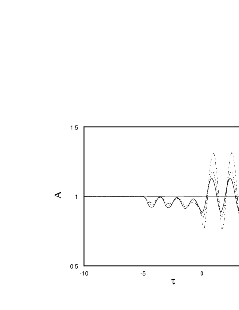
FIG. 2.: $\tau$-$A$ diagram of the $n=2$ mode for the $0<\gamma<1$ case. We set $\alpha/r_{I}=1$ and $\gamma=0.2$ (dot-dashed line),  $0.4$ (dashed line), $0.6$ (solid line). The ingoing flux is turned on at $\tau=-\tau_{0}=-5$. Both $A$ and $\dot{A}$ are finite even on the CH ($\tau=0$). Hence we can define the Bogoliubov coefficients in the $\tau\to 0$ region.

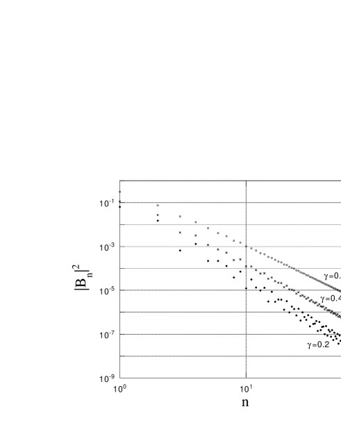
FIG. 3.: The Bogoliubov coefficient for each $n$ mode and different parameters $\gamma$. We can see that the Bogoliubov coefficients decrease faster than $\sim n^{-2}$ for $0<\gamma<1$.

Finally we show the expectation value of the mass-squared operator in Fig. 4. ${\langle{M^{2}}_{\rm{out}}\rangle}_{N}$ means that the sum is taken up to $N$. Hence the real expectation value is realized in the $N\to\infty$ limit. As we expected, ${\langle{M^{2}}_{\rm{out}}\rangle}_{N}$ converges for each $\gamma$, which means that the excitation of the string is finite. Hence the string can smoothly pass through the CH for $0<\gamma<1$, i.e. $\kappa_{I}<2\kappa$.

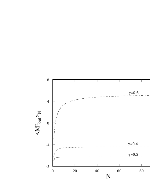
FIG. 4.: The expectation value of the mass-squared operator for different parameters $\gamma$. We can see that ${\langle{M^{2}}_{\rm{out}}\rangle}_{N}$ approaches a constant value in the $N\to\infty$ limit, which means that the expectation value of the mass-squared operator is finite for $0<\gamma<1$. Hence the test string can pass across the CH.

V Concluding remarks

We have examined whether a null weak singularity inside generic charged black holes is a real end of spacetime in terms of a first-quantized test string by using a charged Vaidya model. In an asymptotically flat spacetime ($\Lambda=0$ case), the first-quantized test string falling into the CH is always excited infinitely, while it is not when $\kappa_{I}<2\kappa$ in an asymptotically de Sitter spacetime ($\Lambda>0$ case), in spite of the existence of a p.p. curvature singularity along the CH. We should note that the latter case occurs in the physically relevant range of parameters $m>q$. This implies that the asymptotically de Sitter spacetime can be extended through the CH and hence that the strong cosmic censorship is violated in string theory.

It is worth commenting that when the string is excited infinitely, one should further consider for the following two points: (i) in general, a second-quantized string theory is necessary for judging whether the CH is the real end of spacetime in string theory; (ii) the plane-wave approximation is violated in the solutions near the CH. As for the first point, however, Horowitz and Steif [8] speculated that there is no “string creation” in the plane-wave metric from the fact that there is no particle creation in the metric [13]. This suggests that the first-quantized description should be adequate in the spacetime under consideration. As for the second point, the typical size of the string grows to infinity as follows [17],

$$<r^{2}>\,\sim\int d\sigma:x^{i}(0,\sigma)^{2}:\,\sim\sum_{i,n}\frac{|B_{n}^{i}|^{2}}{n}\sim\infty,$$ (76)

where $:\,\,:$ denotes the normal ordering required to make the quantum operator well defined. Therefore, it is still an open question how much this violation would affect our results in the asymptotically flat case.

As already mentioned before, the internal structure of generic Kerr-type vacuum black holes is locally quite similar to that of spherically symmetric charged black holes. Thus, as verified in the charged Vaidya model, if the surface gravity of the inner horizon in the generic Kerr-type black holes is small enough, we naively expect that the spacetime near the CH is approximately described by the plane-wave metric,

$$ds^{2}\approx-du\,dv+F(v,x^{i})dv^{2}+dx_{i}dx^{i},$$ (77)

$$F=W_{ij}(v)x^{i}x^{j},$$ (78)

where $W_{ij}(v)$ is symmetric and traceless from the vacuum Einstein equations (here we suppose that the cosmological constant is negligibly small). In this case, the metric is also a metric of the classical solution for string theory [7] and the same result as in the charged Vaidya model would be obtained.

In general, the back reaction from the first-quantized string and the quantum corrections for the background metric should be considered. However, such effects should be very small in the case that a first-quantized test string is not excited infinitely. This strongly suggests that the strong cosmic censorship is violated in an asymptotically de Sitter spacetime in string theory, in contrast to general relativity.

REFERENCES

- [1] R. Penrose, Riv. Nuovo Cimento 1, 252 (1969).
- [2] E. Poisson and W. Israel, Phys. Rev. D 41, 1796 (1990).
- [3] A. Ori, Phys. Rev. Lett. 68, 2117 (1992).
- [4] P. R. Brady and J. D. Smith, Phys. Rev. Lett. 75, 1256 (1995).
- [5] L. M. Burko, Phys. Rev. Lett. 79, 4958 (1997).
- [6] P. R. Brady, C. M. Chambers, Phys. Rev. D 51, 4177 (1995).
- [7] G. T. Horowitz and A. R. Steif, Phys. Rev. Lett. 64, 260 (1990).
- [8] G. T. Horowitz and A. R. Steif, Phys. Rev. D 42, 1950 (1990).
- [9] S. W. Hawking and G. F. R. Ellis, The large scale structure of spacetime (Cambridge University Press, Cambridge, 1973).
- [10] R. Guven, Phys. Lett. B 191, 275 (1987).
- [11] D. Amati and C. Klimcik, Phys. Lett. B 219, 443 (1989).
- [12] G. T. Horowitz and S. F. Ross, Phys. Rev. D 57, 1098 (1998).
- [13] G. W. Gibbons, Commun. Math. Phys. 45, 191 (1975).
- [14] R. H. Price, Phys. Rev. D 5, 2419 (1972).
- [15] P. R. Brady, I. G. Moss, and R. C. Myers, Phys. Rev. Lett. 80, 3432 (1998).
- [16] H. J. de Vega and N. Sánchez, Phys. Rev. D 45, 2784 (1992).
- [17] D. Mitchell and N. Turok, Nucl. Phys. B294, 1138 (1987).